
Optimization of a Fuzzy-Logic-Control-Based MPPT Algorithm Using the Particle Swarm Optimization Technique


Abstract
:
1. Introduction
2. System Configuration

3. Derivation of the Symmetrical FLC-based MPPT Controller


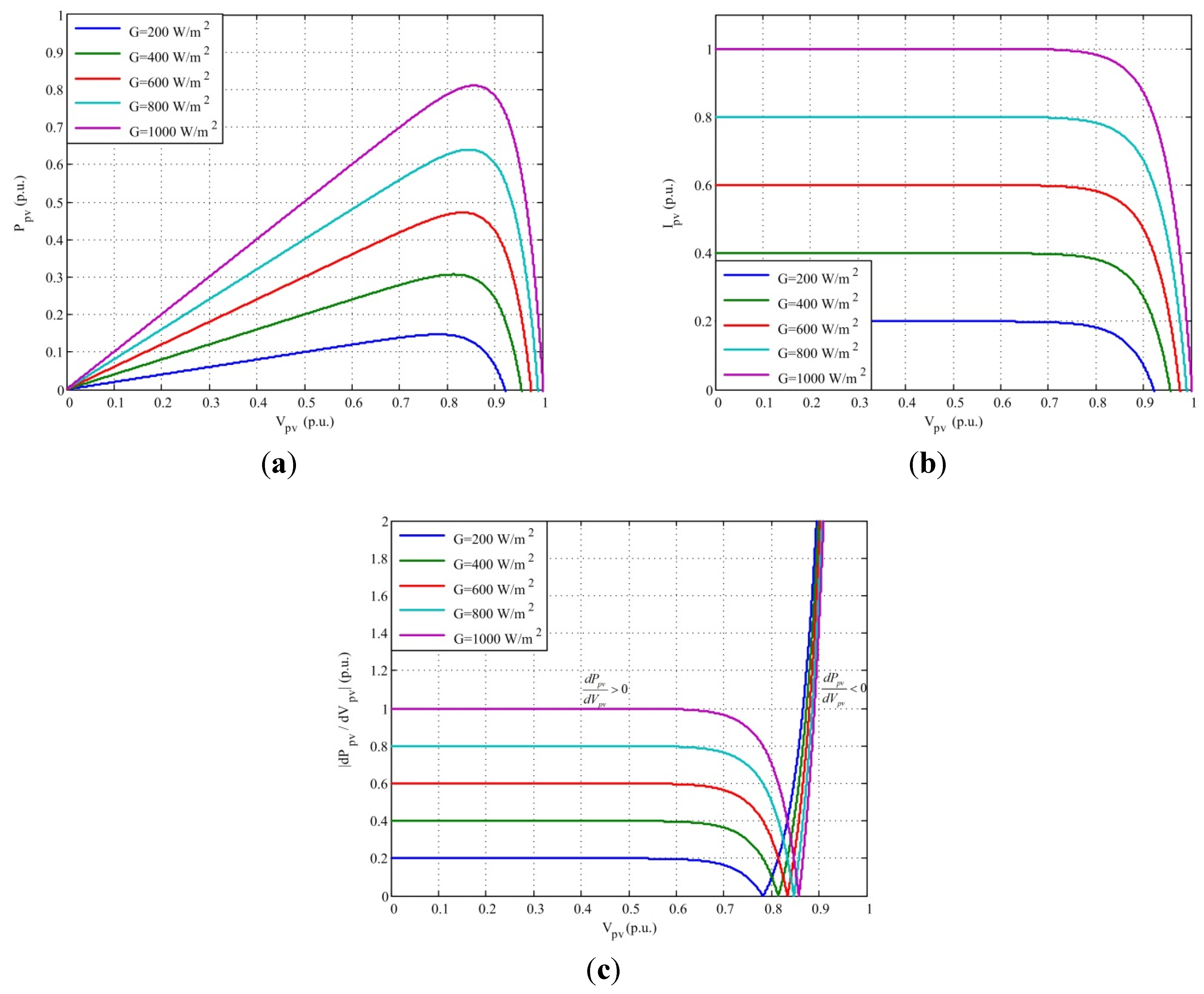
- ΔVpv is zero but ΔPpv does not equal zero, which indicates that the irradiance level has changed (grey arrow in Figure 5). In this situation, the control variable (Vpv) should increase/decrease if ΔPpv is positive (irradiance level increase)/negative (irradiance level decrease); hence ΔVpv is positive/negative. (grey area in Table 1).


| ΔPpv | ΔVpv | ||||
|---|---|---|---|---|---|
| NB | NS | ZE | PS | PB | |
| NB | PS | PB | NB | NB | NS |
| Rule1 | Rule6 | Rule11 | Rule16 | Rule21 | |
| NS | PS | PS | NS | NS | NS |
| Rule2 | Rule7 | Rule12 | Rule17 | Rule22 | |
| ZE | ZE | ZE | ZE | ZE | ZE |
| Rule3 | Rule8 | Rule13 | Rule18 | Rule23 | |
| PS | NS | NS | PS | PS | PS |
| Rule4 | Rule9 | Rule14 | Rule19 | Rule24 | |
| PB | NS | NB | PB | PB | PS |
| Rule5 | Rule10 | Rule15 | Rule20 | Rule25 | |

4. Derivation of the Proposed Asymmetrical FLC-Based MPPT Controller
4.1. Concept of Asymmetrical FLC-Based MPPT Controller

4.2. Systematic Approach to Determine the MF Setting Values of ∆Ppv

5. PSO-based Approach to Determine the optimized MF Setting Values of ∆Ppv

5.1. Basic Concept of PSO

5.2. Application of PSO to Optimize the MF Setting Values of ∆Ppv
- Maximize FLC_Fit_value (dP_PB, dP_PS, dP_NS, dP_NB)
- Subject to dP_PB > dP_PS > 0, 0 > dP_NS > dP_NB, dP_PB < POSmax and dP_NB > NEGmax

5.3. The obtained Optimal MF Setting


6. Experimental Results
| PV Model Sanyo VBHN220AA01 | |||
|---|---|---|---|
| Maximum Power (Pmax) | 220 W | Short Circuit Current (Isc) | 5.65 A |
| Open Circuit Voltage (Voc) | 52.3 V | Maximum Power Current (Imp) | 5.17 A |
| Maximum Power Voltage (Vpm) | 42.7 V | Temperature Coefficient (αv) | −0.336%/°C |
| Specification | Designed Parameter | ||
|---|---|---|---|
| Input Voltage | Vin = 20~70 V | Kp | 0.1 |
| Rated Output Voltage | Vo = 100 V | Ki | 0.008 |
| Rated Ouput Current | Io = 3 A | L1 | 2 mH |
| Rated Output Power | Po = 300 W | C1 | 66 μF |
| Switching Frequency | fs = 50 kHz | Q1 | IRFP460 |
| Output Voltage Ripple | ∆Vo/Vo = < 1% | D1 | STPS20150CT |
| No. | Description | Parameters | Note |
|---|---|---|---|
| 1 | P&O (∆V = 0.5 V) | Fixed Perturbation Step | denoted as method 1 |
| 2 | P&O (∆V = 3.5 V) | Fixed Perturbation Step | denoted as method 2 |
| 3 | Symmetrical FLC | dP_PB = 8.4 W dP_NB = −8.4 W dV_PB = 1.5 V dV_NB = −1.5 V | denoted as method 3 |
| 4 | Asymmetrical FLC #1 | dP_PB = 0.78 W dP_NB = −8.4 W dP_PS = 0.39 W dP_NS = −4.2 W dV_PB = 1.5 V dV_NB = −1.5 V | denoted as method 4 Parameters from Section 4.2 |
| 5 | Asymmetrical FLC #2 | dP_PB = 1.17 W dP_NB = −10.32 W dP_PS = 0.55 W dP_NS = −0.19 W dV_PB = 1.5 V dV_NB = −1.5 V | denoted as method 5 Parameters from Section 5.2 |


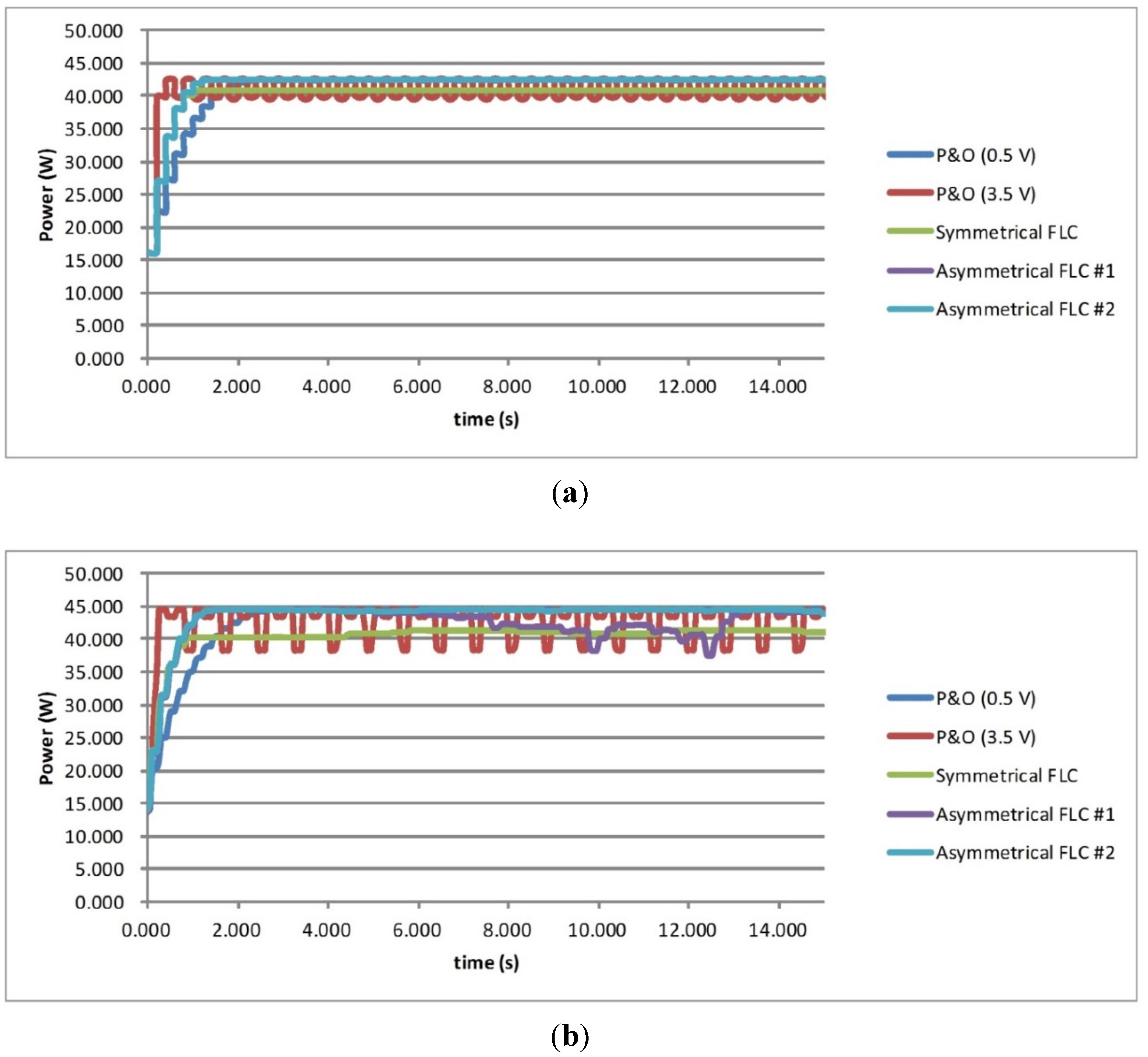
| Real PMPP = 44.8 W | Average steady state output power | MPPT tracking accuracy | Transient time |
|---|---|---|---|
| P&O (0.5 V) | 44.10 W | 98.44% | 1.45 s |
| P&O (3.5 V) | 42.71 W | 95.33% | 0.25 s |
| Symmetrical FLC | 41.57 W | 92.78% | 0.90 s |
| Asymmetrical FLC #1 | 42.87 W | 95.70% | 0.85 s |
| Asymmetrical FLC #2 | 44.12 W | 98.48% | 0.70 s |
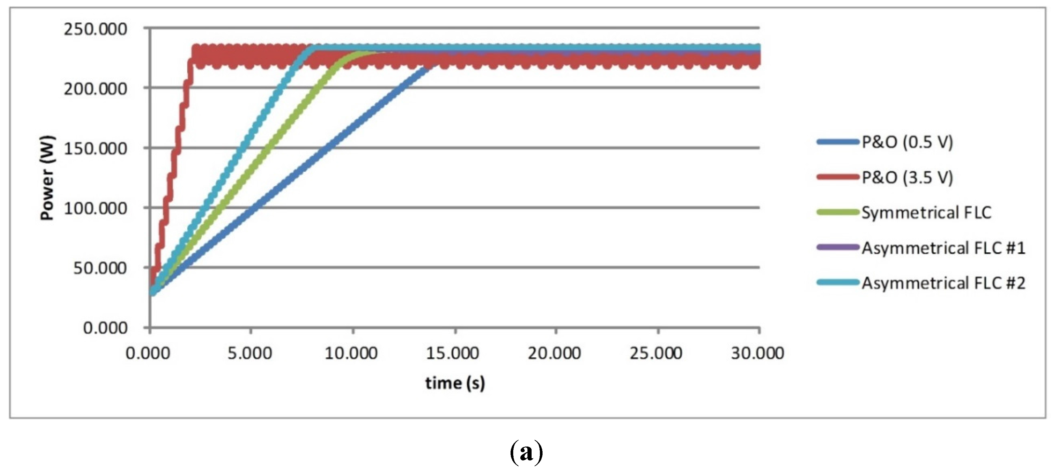
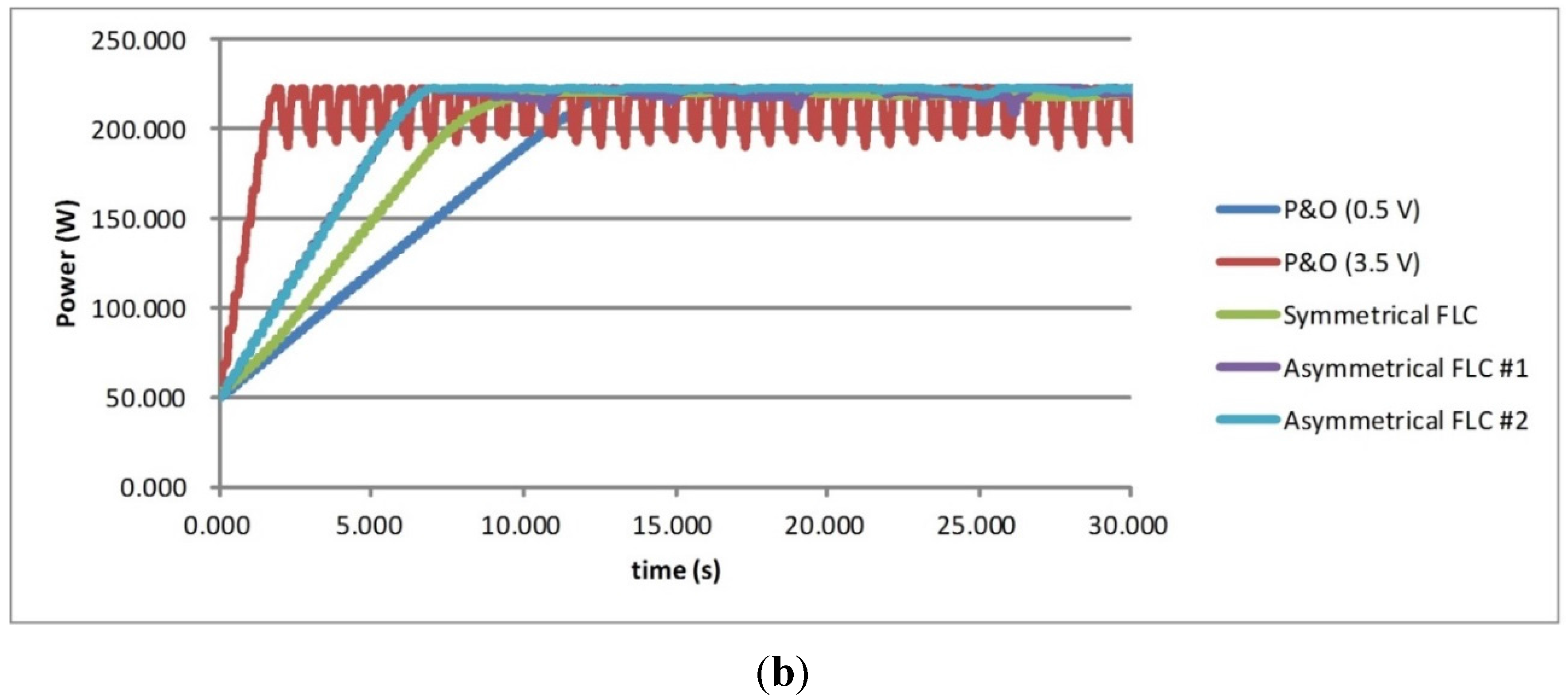
| Real PMPP = 224 W | Average steady state output power | MPPT tracking accuracy | Transient time |
|---|---|---|---|
| P&O (0.5 V) | 222.12 W | 99.16% | 10.75 s |
| P&O (3.5 V) | 212.55 W | 94.89% | 1.50 s |
| Symmetrical FLC | 220.11 W | 98.21% | 7.55 s |
| Asymmetrical FLC #1 | 219.98 W | 98.26% | 5.65 s |
| Asymmetrical FLC #2 | 222.18 W | 99.19% | 5.60 s |
| MPPT methods | Simulated results | Experimental results |
|---|---|---|
| P&O (0.5 V) | 94.58% | 96.12% |
| P&O (3.5 V) | 94.97% | 96.11% |
| Symmetrical FLC | 72.48% | 73.46% |
| Asymmetrical FLC #1 | 96.54% | 96.82% |
| Asymmetrical FLC #2 | 97.11% | 97.69% |
7. Conclusions
Acknowledgments
Author Contributions
Conflicts of Interest
References
- Lee, J.S.; Lee, K.B. Variable DC-link voltage algorithm with a wide range of maximum power point tracking for a two-string PV system. Energies 2013, 6, 58–78. [Google Scholar] [CrossRef]
- Shen, C.L.; Tsai, C.T. Double-linear approximation algorithm to achieve maximum-power-point tracking for photovoltaic arrays. Energies 2012, 5, 1982–1997. [Google Scholar] [CrossRef]
- Yau, H.T.; Wu, C.H. Comparison of extremum-seeking control techniques for maximum power point tracking in photovoltaic systems. Energies 2011, 4, 2180–2195. [Google Scholar] [CrossRef]
- Sera, D.; Kerekes, T.; Teodorescu, R.; Blaabjerg, F. Improved MPPT Algorithms for Rapidly Changing Environmental Conditions. In Proceedings of Power Electronics and Motion Control, Portoroz, Slovenia, 30 August–1 September 2006; pp. 1614–1619.
- Chen, Y.T.; Lai, Z.H.; Liang, R.H. A novel auto-scaling variable step-size MPPT method for a PV system. Sol. Energy 2014, 102, 247–256. [Google Scholar] [CrossRef]
- Radjaia, T.; Rahmania, L.; Mekhilefb, S.; Gaubertc, J.P. Implementation of a modified incremental conductance MPPT algorithm with direct control based on a fuzzy duty cycle change estimator using dSPACE. Sol. Energy 2014, 110, 325–337. [Google Scholar] [CrossRef]
- Abdelsalam, A.K.; Massoud, A.M.; Ahmed, S.; Enjeti, P. High-Performance Adaptive Perturb and Observe MPPT Technique for Photovoltaic-Based Microgrids. IEEE Trans. Power Electron. 2011, 26, 1010–1021. [Google Scholar] [CrossRef]
- Liu, F.; Duan, S.; Liu, F.; Liu, B.; Kang, Y. A Variable Step Size INC MPPT Method for PV Systems. IEEE Trans. Ind. Electron. 2008, 55, 2622–2628. [Google Scholar]
- Pandey, A.; Dasgupta, N.; Mukerjee, A.K. High-Performance Algorithms for Drift Avoidance and Fast Tracking in Solar MPPT System. IEEE Trans. Energy Convers. 2008, 23, 681–689. [Google Scholar] [CrossRef]
- Mei, Q.; Shan, M.W.; Liu, L.Y.; Guerrero, J.M. A Novel Improved Variable Step-Size Incremental-Resistance MPPT Method for PV Systems. IEEE Trans. Ind. Electron. 2011, 58, 2427–2434. [Google Scholar] [CrossRef]
- Messai, A.; Mellit, A.; Massi Pavan, A.; Guessoum, A.; Mekki, H. FPGA-based implementation of a fuzzy controller (MPPT) for photovoltaic module. Energy Convers. Manag. 2011, 52, 2695–2704. [Google Scholar] [CrossRef]
- Larbes, C.; Ait Cheikh, S.M.; Obeidi, T.; Zerguerras, A. Genetic algorithms optimized fuzzy logic control for the maximum power point tracking in photovoltaic system. Renew. Energy 2009, 34, 2093–2100. [Google Scholar] [CrossRef]
- Messai, A.; Mellit, A.; Guessoum, A.; Kalogirou, S.A. Maximum power point tracking using a GA optimized fuzzy logic controller and its FPGA implementation. Sol. Energy 2011, 85, 265–277. [Google Scholar] [CrossRef]
- Letting, L.K.; Munda, J.L.; Hamama, Y. Optimization of a fuzzy logic controller for PV grid inverter control using S-function based PSO. Sol. Energy 2012, 86, 1689–1700. [Google Scholar] [CrossRef]
- Kottas, T.L.; Boutalis, Y.S.; Karlis, A.D. New maximum power point tracker for PV arrays using fuzzy controller in close cooperation with fuzzy cognitive networks. IEEE Trans. Energy Convers. 2006, 21, 793–803. [Google Scholar] [CrossRef]
- Algazar, M.M.; AL-monier, H.; EL-halim, H.A.; Salem, M.E.E.K. Maximum power point tracking using fuzzy logic control. Int. J. Electron. Power Energy Syst. 2012, 39, 21–28. [Google Scholar] [CrossRef]
- Shiau, J.K.; Lee, M.Y.; Wei, Y.C.; Chen, B.C. Circuit Simulation for Solar Power Maximum Power Point Tracking with Different Buck-Boost Converter Topologies. Energies 2014, 7, 5027–5046. [Google Scholar] [CrossRef]
- Guenounou, O.; Dahhou, B.; Chabour, F. Adaptive fuzzy controller based MPPT for photovoltaic systems. Energy Convers. Manag. 2014, 78, 843–850. [Google Scholar] [CrossRef]
- Bendiba, B.; Krimb, F.; Belmilia, H.; Almia, M.F.; Bouloumaa, S. Advanced Fuzzy MPPT Controller for a stand-alone PV system. Energy Procedia 2014, 50, 383–392. [Google Scholar] [CrossRef]
- Altin, N.; Ozdemir, S. Three-phase three-level grid interactive inverter with fuzzy logic based maximum power point tracking controller. Energy Convers. Manag. 2013, 69, 17–26. [Google Scholar] [CrossRef]
- Mohd Zainuri, M.A.A.; Mohd Radzi, M.A.; Soh, A.C.; Rahim, N.A. Development of adaptive perturb and observe-fuzzy control maximum power point tracking for photovoltaic boost DC-DC converter. Renew. Power Gener. IET 2014, 8, 183–194. [Google Scholar] [CrossRef]
- Mozaffari Niapour, S.A.KH.; Danyali, S.; Sharifian, M.B.B.; Feyzi, M.R. Brushless DC motor drives supplied by PV power system based on Z-source inverter and FL-IC MPPT controller. Energy Convers. Manag. 2011, 52, 3043–3059. [Google Scholar] [CrossRef]
- Ravi, A.; Manoharan, P.S.; Vijay Anand, J. Modeling and simulation of three phase multilevel inverter for grid connected photovoltaic systems. Sol. Energy 2011, 85, 2811–2818. [Google Scholar] [CrossRef]
- Lalouni, S.; Rekioua, D.; Rekioua, T.; Matagne, E. Fuzzy logic control of stand-alone photovoltaic system with battery storage. J. Power Sour. 2009, 193, 899–907. [Google Scholar] [CrossRef]
- Alajmi, B.N.; Ahmed, K.H.; Finney, S.J.; Williams, B.W. Fuzzy-logic-control approach of a modified hill-climbing method for maximum power point in microgrid standalone photovoltaic system. IEEE Trans. Power Electron. 2011, 26, 1022–1030. [Google Scholar] [CrossRef]
- Alajmi, B.N.; Ahmed, K.H.; Finney, S.J.; Williams, B.W. A maximum power point tracking technique for partially shaded photovoltaic systems in microgrids. IEEE Trans. Ind. Electron. 2013, 60, 573–584. [Google Scholar] [CrossRef]
- Alajmi, B.N.; Ahmed, K.H.; Adam, G.P.; Williams, B.W. Single-phase single-stage transformer less grid-connected PV system. IEEE Trans. Power Electron. 2013, 28, 2664–2676. [Google Scholar] [CrossRef]
- Subiyanto, S.; Mohamed, A.; Hannan, M.A. Intelligent maximum power point tracking for PV system using Hopfield neural network optimized fuzzy logic controller. Energy Build. 2012, 51, 29–38. [Google Scholar] [CrossRef]
- Liu, C.L.; Chen, J.H.; Liu, Y.H.; Yang, Z.Z. An Asymmetrical Fuzzy-Logic-Control-Based MPPT Algorithm for Photovoltaic Systems. Energies 2014, 7, 2177–2193. [Google Scholar] [CrossRef]
- Altas, I.H.; Sharaf, A.M. A novel maximum power fuzzy logic controller for photovoltaic solar energy systems. Renew. Energy 2008, 33, 388–399. [Google Scholar] [CrossRef]
- Gounden, N.A.; Peter, S.A.; Nallandula, H.; Krithiga, S. Fuzzy logic controller with MPPT using line-commutated inverter for three-phase grid-connected photovoltaic systems. Renew. Energy 2009, 34, 909–915. [Google Scholar] [CrossRef]
- Syafaruddin; Karatepe, E.; Hiyama, T. Artificial neural network-polar coordinated fuzzy controller based maximum power point tracking control under partially shaded conditions. IET Renew. Power Gener. 2009, 3, 239–253. [Google Scholar] [CrossRef]
- Syafaruddin; Karatepe, E.; Hiyama, T. Polar coordinated fuzzy controller based real-time maximum-power point control of photovoltaic system. Renew. Energy 2009, 34, 2597–2606. [Google Scholar] [CrossRef]
- Chaouachi, A.; Kamel, R.M.; Nagasaka, K. A novel multi-model neuro-fuzzy-based MPPT for three-phase grid-connected photovoltaic system. Sol. Energy 2010, 84, 2219–2229. [Google Scholar] [CrossRef]
- Salah, C.B.; Ouali, M. Comparison of fuzzy logic and neural network in maximum power point tracker for PV systems. Electr. Power Syst. Res. 2011, 81, 43–50. [Google Scholar] [CrossRef]
- Abu-Rub, H.; Iqbal, A.; Ahmed, S.M.; Peng, F.Z.; Li, Y.; Baoming, G. Quasi-Z-source inverter-based photovoltaic generation system with maximum power tracking control using ANFIS. IEEE Trans. Sustain. Energy 2013, 4, 11–20. [Google Scholar] [CrossRef]
- Karlis, A.D.; Kottas, T.L.; Boutalis, Y.S. A novel maximum power point tracking method for PV systems using fuzzy cognitive networks (FCN). Electr. Power Syst. Res. 2007, 77, 315–327. [Google Scholar] [CrossRef]
- Chiu, C.S. T-S fuzzy maximum power point tracking control of solar power generation systems. IEEE Trans. Energy Convers. 2010, 25, 1123–1132. [Google Scholar] [CrossRef]
- Chiu, C.S.; Ouyang, Y.L. Robust maximum power tracking control of uncertain photovoltaic systems: A unified T-S fuzzy model-based approach. IEEE Trans. Control Syst. Technol. 2011, 19, 1516–1526. [Google Scholar] [CrossRef]
- Arulmurugan, R.; Suthanthiravanitha, N. Model and design of a fuzzy-based Hopfield NN tracking controller forstandalone PV applications. Electr. Power Sys. Res. 2015, 120, 184–193. [Google Scholar] [CrossRef]
- Rajesh, R.; Carolin Mabel, M. Efficiency analysis of a multi-fuzzy logic controller for the determination of operating points in a PV system. Sol. Energy 2014, 99, 77–87. [Google Scholar] [CrossRef]
- Nabulsi, A.A.; Dhaouadi, R. Efficiency Optimization of a DSP-Based Standalone PV System Using Fuzzy Logic and Dual-MPPT Control. IEEE Trans. Ind. Inf. 2012, 8, 573–584. [Google Scholar] [CrossRef]
- Shiau, J.K.; Wei, Y.C.; Lee, M.Y. Fuzzy Controller for a Voltage-Regulated Solar-Powered MPPT System for Hybrid Power System Applications. Energies 2015, 8, 3292–3312. [Google Scholar] [CrossRef]
- Erickson, R.W.; Maksimovic, D. Fundamentals of Power Electronics, 2nd ed.; Springer: Berlin, German, 2001. [Google Scholar]
- Parsopoulos, K.E.; Vrahatis, M.N. Particle Swarm Optimization and Intelligence: Advances and Applications, 1st ed.; IGI Global: Hershey, PA, USA, 2010; pp. 25–34. [Google Scholar]
© 2015 by the authors; licensee MDPI, Basel, Switzerland. This article is an open access article distributed under the terms and conditions of the Creative Commons Attribution license (http://creativecommons.org/licenses/by/4.0/).
Share and Cite
Cheng, P.-C.; Peng, B.-R.; Liu, Y.-H.; Cheng, Y.-S.; Huang, J.-W. Optimization of a Fuzzy-Logic-Control-Based MPPT Algorithm Using the Particle Swarm Optimization Technique. Energies 2015, 8, 5338-5360. https://doi.org/10.3390/en8065338
Cheng P-C, Peng B-R, Liu Y-H, Cheng Y-S, Huang J-W. Optimization of a Fuzzy-Logic-Control-Based MPPT Algorithm Using the Particle Swarm Optimization Technique. Energies. 2015; 8(6):5338-5360. https://doi.org/10.3390/en8065338
Chicago/Turabian StyleCheng, Po-Chen, Bo-Rei Peng, Yi-Hua Liu, Yu-Shan Cheng, and Jia-Wei Huang. 2015. "Optimization of a Fuzzy-Logic-Control-Based MPPT Algorithm Using the Particle Swarm Optimization Technique" Energies 8, no. 6: 5338-5360. https://doi.org/10.3390/en8065338