
The Dynamic Impacts of the COVID-19 Pandemic on Log Prices in China: An Analysis Based on the TVP-VAR Model


School of Economics and Management, Beijing Forestry University, Beijing 100083, China
*
Author to whom correspondence should be addressed.
Forests 2021, 12(4), 449; https://doi.org/10.3390/f12040449
Submission received: 11 February 2021
/
Revised: 25 March 2021
/
Accepted: 1 April 2021
/
Published: 7 April 2021
(This article belongs to the Section Forest Economics, Policy, and Social Science)
Abstract
:China’s wood industry is vulnerable to the COVID-19 pandemic since wood raw materials and sales of products are dependent on the international market. This study seeks to explore the speed of log price recovery under different control measures, and to perhaps find a better way to respond to the pandemic. With the daily data, we utilized the time-varying parameter autoregressive (TVP-VAR) model, which can incorporate structural changes in emergencies into the model through time-varying parameters, to estimate the dynamic impact of the pandemic on log prices at different time points. We found that the impact of the pandemic on oil prices and Renminbi exchange rate is synchronized with the severity of the pandemic, and the ascending in the exchange rate would lead to an increase in log prices, while oil prices would not. Moreover, the impulse response in June converged faster than in February 2020. Thus, partial quarantine is effective. However, the pandemic’s impact on log prices is not consistent with changes of the pandemic. After the pandemic eased in June 2020, the impact of the pandemic on log prices remained increasing. This means that the COVID-19 pandemic has long-term influences on the wood industry, and the work resumption was not smooth, thus the imbalance between supply and demand should be resolved as soon as possible. Therefore, it is necessary to promote the development of the domestic wood market and realize a “dual circulation” strategy as the pandemic becomes a “new normal”.
1. Introduction
Wood prices not only affect the supply and demand of wood but also influence the expectations of forest managers and the public on the income of forest land and the choice of forest resource management methods [1]. The coronavirus (COVID-19) pandemic outbreak began in November 2019 and attracted attention in early 2020. In China, cases were exponentially increasing in just a few weeks and even exceeded 80,000 at the beginning of March. Due to effective control measures, the spread of the virus got under control. However, as an international public health emergency, the sharp increase in uncertainty during the coronavirus pandemic had severe implications for the industrial supply chain of China and the world [2,3], and the pandemic might leave its legacy for years to come. According to the China Entrepreneur Investment Club (CEIC) Database, China’s actual GDP decreased by 6.8% in the first quarter of 2020, and the world’s industrial output also decreased by 4.5%. Meanwhile, the pandemic also severely affected the smooth operation of the Chinese wood market [4,5,6]. Simultaneously, according to the China’s Forest Products Import and Export Bulletin in 2020, the unit price of logs in China decreased by 16.3%, and the unit price of sawn lumber decreased by 9.9% from January to March 2020. However, in May and June, wood prices rebounded. Overall, China’s wood prices fluctuated sharply during the first half of 2020. Understanding the impact of the pandemic on wood prices and clarifying the internal mechanism is necessary to help and guide the wood market to return to orderly development. It also has specific referencing significance for other countries and responding to future international emergencies.
COVID-19 had varied impacts on different industries, which caused some hoarding and a short-term fluctuation in prices [2]. Market supply is insufficient to meet demand because of disruption in transportation, leading to an increase in the price of food and other agricultural products, and some specific products, like medical care [7,8,9,10]. Nevertheless, the total social demand for some products decreased, so the price of coal and some mining products, and some tourism service products such as airlines and hotels dropped sharply [7,8,11,12,13]. However, few scholars focus on the impact of the pandemic on log prices. China has limited domestic lumber resources with clearly not enough to supply domestic demand. Filling this wood gap depends on imports. Furthermore, owing to the irregular and uneven shape of lumber, and the heavy weight, the transportation is costly. Consequently, China’s wood pricing is highly dependent on the exchange rate and transportation costs [14,15,16,17]. In addition, the wood industry’s profit is typically low with a simple value chain [18], and most wood companies are small or medium-sized enterprises [19,20]. Therefore, volatility in wood prices caused by the pandemic influences the cost of manufacture and is a major concern for the wood industry [21]. By the end of March 2020, only 10.9% of wood companies maintained a relatively stable production, while others were all facing operational difficulties or even bankruptcy [22]. In this case, it is particularly important to restore log price stability as soon as possible, which is why we want to clarify the relationship between the pandemic and log prices. Another issue is that the pandemic has had a period of rapid deterioration (hereinafter referred to as the “early phase”) and a stable recovery period (hereinafter referred to as the “late phase”), and there has also been a second outbreak in June. At different stages of the pandemic, there are differences regarding the public’s mood, psychology, social and economic conditions, and so on. Thus, the importance to make sure how the COVID-19 pandemic affects log prices differently and what the best response mechanism is between the different phases.
This paper uses a time-varying parameter autoregressive (TVP-VAR) model to study the interaction between the COVID-19 pandemic and log prices based on daily frequency data. It allows us to judge the impact of the pandemic on log prices in different periods, and then provide a basis for industrial adjustment. The rest of the paper presents the hypothesis (Section 2), methodology and data (Section 3), the empirical findings (Section 4), and the discussion (Section 5). Finally, we conclude.
2. Hypothesis
Decomposing the total effects of one variable on another into direct and indirect effects has long been of interest to researchers [23]. In terms of direct impacts, COVID-19 influences the wood supply and demand market, leading to changes in log prices. Regarding indirect effects, the pandemic affects log prices by affecting oil prices and exchange rates.
In terms of price composition, the delivery cost of log is high. For instance, the transportation cost of lumber accounts for nearly 25% of the delivery price of low-value lumber [24]. Furthermore, China’s demand gap for lumber in 2020 may reach 200 million cubic meters. Nearly 50% of wood comes from imports, and most international wood trade is priced in US dollars. Therefore, the price of log is indirectly affected by oil prices and the exchange rate. Accordingly, we propose the following research hypotheses.
Hypothesis 1 (H1).
If only considering oil prices, the COVID-19 pandemic would impact log prices first decreasingly and then increasingly.
Transportation is vital in the wood supply chain [24], and the price of crude oil is one of the essential factors affecting transportation costs. According to the price structure, transportation cost is a crucial factor affecting log prices. In the early phase, as part of social distancing policies, the Chinese Government encouraged people to stay at home, discouraged mass gatherings, canceled or postponed significant public events, and closed schools, universities, libraries, cinemas, and factories. Accordingly, oil demand decreased, a large number of petrochemical enterprises suspended production, and oil prices would fall. The cost of marine fuel oil used to transport log would fall. Moreover, the delivery price would also decrease. Log prices may go down as a result [25]. Since March, the pandemic has been basically under control. China safely reopened its production, and oil demand gradually resumed, which may cause oil prices to recover. Moreover, expenditure costs such as personnel salaries and virus prevention materials increased transportation costs [24,26,27]. Again, we expect these increases will be reflected in an increase in log prices. Therefore, changes in oil prices caused by the pandemic are expected to affect changes in log prices in a similar direction.
Hypothesis 2 (H2).
The COVID-19 pandemic would have an ascending impact on log prices by affecting exchange rates, but the degree of impact would vary with time.
Due to the exchange rate pass-through (ERPT) effect, log prices response in correlation with changes in the exchange rate [28]. According to the global provider of secure financial messaging services (SWIFT), although the influence of some kinds of currency such as Euro is increasing, the US’s share as a global currency in trade finance market is still really high, with 87.06%. The US dollar works as the settlement currency of most international trade, and imported lumber is no exception. Therefore, we pay attention to the renminbi/dollar exchange rate. At the beginning, the economic growth and market investment confidence was hit since the public is in panic and frustration [29,30]. According to the theory of Balance of International Payments (BOP), short-term capital flows out, there is a decrease in foreign exchange reserves, and then the RMB depreciates, leading, at last, to local price increases. Therefore, in the early phase, the pandemic caused the depreciation of the RMB and then log prices would increase. When the spread of novel coronavirus slowed down across China, domestic investment confidence would rebound, and short-term capital would flow in, and the RMB depreciation would come under control [31,32]. The impact of the pandemic on the devaluation of the RMB would decrease, and the impact on log prices would be also reduced.
We can analyze not only from the indirect effects but also direct impacts from the perspective of market supply and demand. According to the Equilibrium Theory, in the absence of an external shock, the wood market tends to be in equilibrium under the dual effects of supply and demand [33,34]. In the event of an external shock, such as the occurrence of emergencies just like COVID-19, downstream manufacturers would adjust their decision-making behaviors based on the information they have and change consumption plans such as log purchases, so as to shift the demand curve and affect log prices. Additionally, external shocks may also affect the production plans of upstream manufacturers and the stability of transportation. It may also change the supply of log in the market, which would shift the supply curve and affect log prices [3,35,36].
Hypothesis 3 (H3).
The COVID-19 pandemic would firstly cause log prices to descend sharply, and as the pandemic eases, it would cause log prices to ascend.
The impact of COVID-19 on log prices varies with time. The pandemic reduced total consumption, which in turn affects the market demand for most wood furniture, wood flooring, some paper products, and construction. This would cause wood processing, wood furniture, and paper manufacturers to respond accordingly to avoid inventory backlogs and reduce forest product production. Therefore, the demand for wood materials would decrease, and the demand curve would shift to the left. Log prices may decrease as a result. In contrast, the pandemic also would have an impact on international trade, and the obstruction of international trade influences the supply of China’s wood market. That is, the supply curve would also shift to the left, and log prices may rise. The two forces are in contradiction, and the final change in the price of log would depend on the side with the dominant force. Nevertheless, as time went by, the situation would become different, and the strengths of the two would be also different. In the early phase, according to Trade Data Monitor database, China’s major wood products exports plummeted by 65.7% in February 2020. The demand market was more affected by the pandemic than the supply market, and log prices would fall. Before the resumption of economic activity, the national panic eased, but because factories did not quickly reopen, there was little willingness to trade log. Thus, early changes in the pandemic had less impact on log prices. As new cases of COVID-19 were on a downward trend in China, the factory gradually resumed production, and the domestic consumption of forest products increased. However, according to Trade Data Monitor, due to the deterioration of the world pandemic situation, China’s wood imports have been severely blocked with a descend more than 22.78% in the first half of 2020, especially log decreased by 28.75%. The impact on the supply market would become increasingly prominent. Consequently, log prices may recover or even rise.
3. Methodology and Data
3.1. Methodology
The time-varying parameter autoregressive (TVP-VAR) model can just achieve the goal of this research. Social policies and economic environments change rapidly during the COVID-19, and the relationship between the COVID-19 and log prices is obviously varying as time goes on. The results of ordinary fixed parameter models are unstable. In contrast, the TVP-VAR model can capture the relationship and characteristics of variables in different contexts [37], and incorporate structural changes in emergencies into the model through time-varying parameters. Moreover, the TVP-VAR model does not have the same variance assumption [38], which is more in line with the actual situation. The research results could be, therefore, more realistic.
The basic vector autoregressive (VAR) model is as follows:
This paper involves a total of 4 variables, namely, the COVID-19, international oil prices, exchange rate, and Chinese log prices. Therefore, is a 4 × 1 vector, is a 4 × 4 matrix of coefficients, and is a structural impact, which is also a 4 × 1 vector. The above formula can be rewritten as the following form:
Among them, . And have .
It can be rewritten as
Among them, means Kronecker product.
Furthermore, taking into account the time changes of the parameters, we obtain the time-varying parameter vector autoregressive (TVP-VAR) model [39], which breaks the assumption that the estimated coefficients of the traditional VAR model are constant, and can analyze the nonlinear relationship between variables more accurately. The model form is as follows:
In the formula, the coefficient , parameter , and matrix all change with time. Let denote the stacked vector of lower triangular elements in matrix , and let H be the logarithmic random volatility matrix. Suppose , and for all , the parameters of the TVP-VAR model obey random walks. Suppose they are first-order random walk processes, which is
Assume that , , , obey:
where , , . Assume that the impacts of time-varying parameters are uncorrelated, and that , , are all diagonal matrices. The estimation of the model in this paper is done by the Markov Chain Monte Carlo (MCMC) method [38].
3.2. Data
The phase of the pandemic can be judged based on changes in the number of confirmed COVID-19 cases. Although the data may be affected by political and standard rules and may bring some errors, the number of newly confirmed COVID-19 cases can be verified by the cumulative number of cases and the number of newly confirmed cases in various provinces (regions). Thus, the data is relatively reliable. Therefore, this paper selected the number of newly confirmed COVID-19 cases on the Chinese mainland during the first half of 2020 to represent the COVID-19 pandemic (CO). The data were retrieved from the “Daily Epidemic Bulletin” of the Publicity Department of the National Health Commission of the People’s Republic of China.
Transportation cost is an essential factor affecting log prices, because wood raw materials are bulky and relatively fixed in shape [25], and the main transportation way to import log is by sea in China [40]. A potential increase in oil prices could increase transport costs two-to-eight-fold [41,42]. Some fixed costs also play an important role in transport costs, while in this paper, we only considered about the first half of 2020 and used daily data. The period is short, so, these costs do not change seriously. Therefore, oil price contributes a significant part to transportation cost [43] in this period. Moreover, a rise in oil price gets translated into higher prices for consumption goods, because of consequential rise in their transportation costs [25]. This article chose the Brent daily price as a proxy variable for international crude oil prices (BR). The data were retrieved from the US Energy Information Administration (EIA).
In the foreign exchange market, international investors expect a certain exchange rate appreciation or depreciation by observing the nominal exchange rate of the country’s currency. Therefore, this paper selected the exchange rate of RMB against the US dollar using the direct pricing method as the proxy variable of the exchange rate (EX) [44]. The data came from the website of the People’s Bank of China.
The wood supply chain is a complex network consisting of log supply, log processing, raw material procurement, product manufacturing, product distribution and retail, and end users. Log is the foundation of the supply chain. Logs are the raw materials for most forest products [45]. Therefore, the prices of log and finished products are not exactly the same, but the trend of log prices may affect the price change of wood products [46]. Moreover, log prices are very important for public land managers, woodland investors, and lumber companies [46,47], and it may be the most direct way to monitor the wood markets [47]. Lots of researchers are interested in it [48,49]. Thus, this paper also took the log prices as the research object. We selected the log index of China’s wood price index as the proxy variable of China’s log price (WO). The log index of China’s wood Price Index is one of the 12 crucial commodity and service price indexes compiled and released by the National Development and Reform Commission. In order to get these indexes, investigators go to the sites in different markets every day to register and verify the sales volume and sales price of products. Then, the sum of the total sales volume of one product is used as the sales volume of this product. The price of the commodity selects the transaction price of the product with the largest sales volume ratio. Last but not least, staff use the Weight Harmonic Average (WHA) to calculate the log index of China’s wood Price Index, and so on. The data were between 1 January and 30 June, 2020, and came from the Wind database and China’s Wood Price Index website.
In addition, this paper used multiple imputation methods to impute and fill missing values in the data to ensure the validity and accuracy of the results. Since the data used in this paper was daily data from 1 January to 30 June 2020, which had a short time, seasonality and periodicity can be ignored. Therefore, there was nospecial treatment.
4. Empirical Results and Discussions
4.1. Unit Root Test
The data used in this article were time series, and the stationarity of the data was one of the prerequisites for regression accuracy. We tested the stationarity properties of our series using the augmented Dickey–Fuller (ADF) test where the alternative hypothesis was stationary. According to Schwert [50], the maximum lag order was 13. The ADF test revealed, as mentioned in Table 1, non-stationarity in original sequence where the null hypothesis of the existence of a unit root could not be rejected for any series at original level. The original sequences of four variables were non-stationarity. However, the return series showed stationarity at 10% significance level, implying that they were integrated of order 1. It illustrates that the four series of the COVID-19, international oil prices, exchange rate, and China’s log prices were all the I (1) process, which met the data requirements of the TVP-VAR model.
4.2. Estimation Results by MCMC
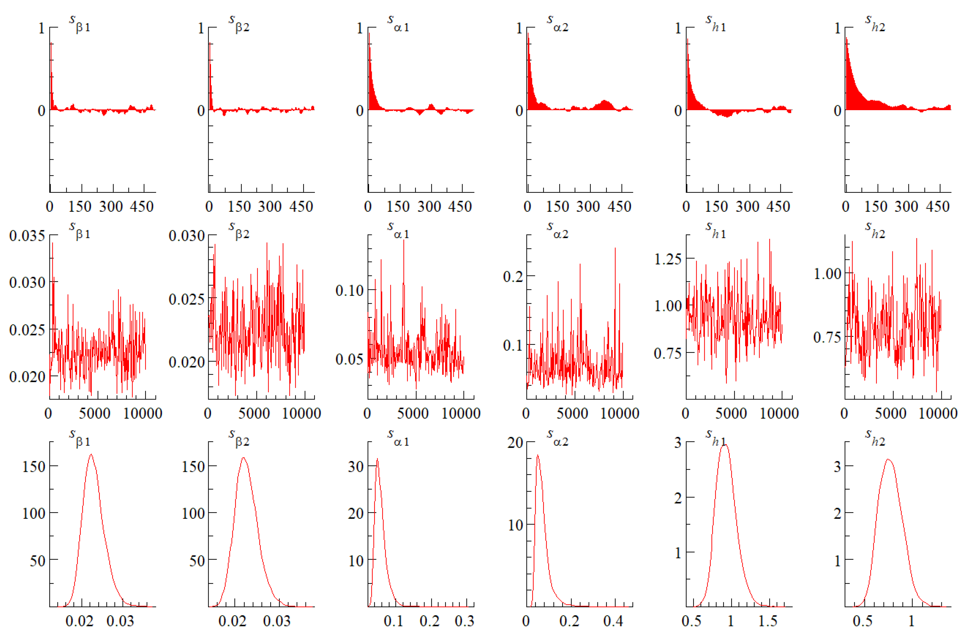
According to Lütkepohl [51], the HQIC provided a consistent estimate of the correct lag order, and the lag order used for this research was set to 3. Before using the Markov Chain Monte Carlo (MCMC) method to simulate, we needed to set the initial values of the parameters in advance. This paper referred to the method of Nakajima et al. [38] to set the initial values: , , , , , . This paper used OxMetrics to execute the MCMC algorithm for 10,000 samplings and discards the first 1000 samplings, thereby obtaining valid samples for model posterior estimation. The parameter estimates of the TVP-VAR model can change over time. The first line of Figure 1 shows the autocorrelation function of the sample. In the displayed 500 samples, the autocorrelation of the sample decreased steadily. The second line shows the sample value path. We found that each variable’s sample value fluctuated around the mean, which was not entirely random. The third line shows the density function of the posterior distribution. In general, Figure 1 shows that after discarding the samples in the burn-in period, the degree of the autocorrelation of variables decreased, indicating that the sample value method could effectively generate uncorrelated samples and ensure the accuracy of the simulation results.
Table 2 shows the posterior distribution mean, standard deviation, 95% confidence interval, CD convergence diagnostic value, and invalid factor. The probability of Geweke diagnostic value was greater than 5%, indicating that at the 95% significance level, the null hypothesis of parameter convergence posterior distribution could not be rejected, indicating that the pre-burning period was sufficient to make the Markov chain tend to be concentrated; the invalid factors were all lower than 100, it indicates that the model had generated enough uncorrelated samples for the parameters, and the model estimation was effective.
4.3. Time-Varying Impulse Analysis of Equal Interval
The estimation results of the TVP-VAR model have time-varying characteristics. Its impulse response function includes two types: impulse analysis of equal interval (also called impulse analysis of different time horizons) and impulse analysis of different points, which can simulate the time-varying relationship between variables from the perspective of the time change. The impulse analysis of equal interval shows the response of the dependent variable at different time points in the same lag period after the shock of one-unit standard deviation is generated for the independent variable at all time points, and then compares and analyzes the difference of the influence of dependent variable at different time points. Since this study is based on daily data, Figure 2, Figure 3 and Figure 4 the impulse response of equal interval for a one-day horizon, a one-week horizon, and a two-week horizon. That is 1 day, 7 days, and 14 days described by solid lines, long dashed lines, and short dashed lines, respectively. These three lines correspond to the dependent variable’s impulse response after the short-term, mid-term, and long-term, respectively. As shown in the figures below, the three different lag periods’ impulse responses have some differences in the magnitude and direction. As the number of lag periods increases, the impulse response gradually weakens.
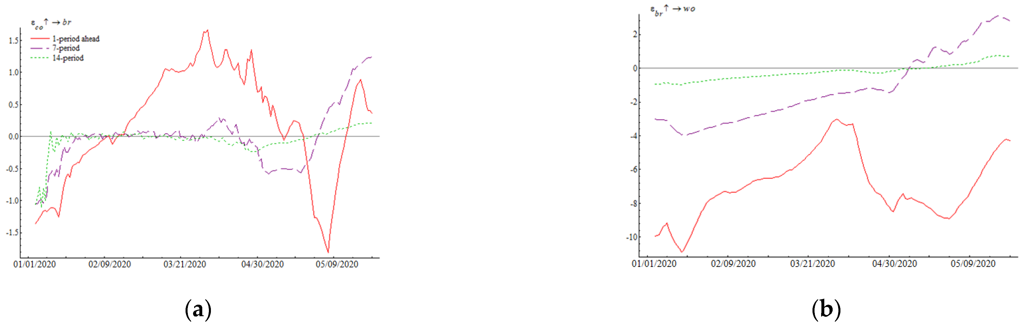
Figure 2a shows that the impulse response of international oil prices to the COVID-19 pandemic was relatively small, mainly between −1 and 1. After reaching the maximum, the response decreased to the minimum in June and then increased again. This result means that although the pandemic was not the main reason for changes in oil prices, at the beginning of 2020, nearly all parts of China imposed social distancing policies to combat the spread of the virus. These policies reduced the number of vehicles traveling and the demand for fuel oil. Meanwhile, a large number of petrochemical companies halted work and production, which further reduced the need for crude oil, leading to a drop in international oil prices. Since March, the pandemic was brought under control. People gradually got back to work, and the demand for crude oil increased, resulting in a recovery in oil prices. With the control measures of the pandemic, the impulse response gradually converged, and the speed of convergence was the same as the rate of change in the number of newly diagnosed COVID-19. It indicates if the pandemic is controlled, the oil industry can resume production. In June, the imported salmon in Beijing Xinfadi Market caused hundreds of infections. Uncertainty in China suddenly increased, and the impulse response of oil prices fluctuated again. Comparing the impulse response in June with that at the beginning of 2020, the impulse responses of crude oil prices were both around −1.5, but obviously, the impulse response in June converges faster. It illustrates that both of outbreaks influenced the crude oil industry, and under more effective government measures, outbreaks were more quickly brought under control. The impulse analysis results of the lagging period in 1, 7, and 14 days of the log prices in Figure 2b shows that the impact of international oil price on log price was descending in the short-term, while it tended to be zero in the mid-term and long-term. It suggests that the rise in international oil prices in the first half of 2020 would not significantly increase log prices in the short term. Considering the two effects, the impact of the COVID-19 pandemic on log prices through international oil price was ascending first, then descending, and finally ascending again in June.
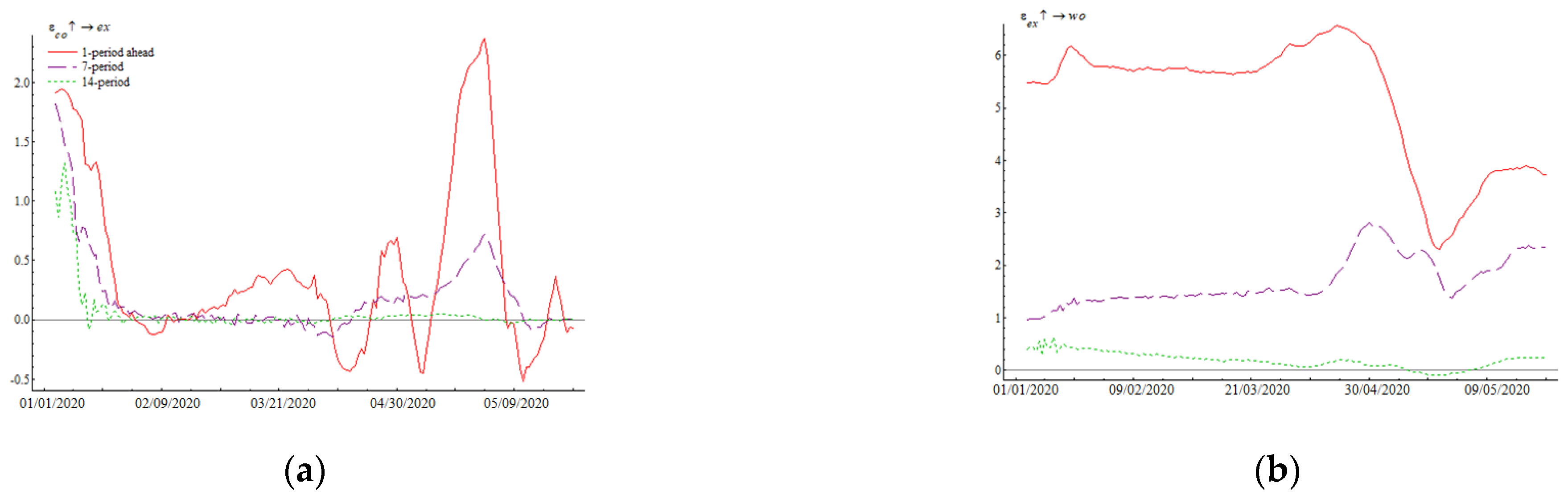
Figure 3a shows a similar trend among the short-term, mid-term, and long-term lagging responses of the exchange rate to the COVID-19. They all showed ascending values since the first outbreak, and then quickly fell back to fluctuations around zero, and suddenly reached the maximum again in June and then fell back. This result suggests that at the beginning of 2020, the increase in the number of people diagnosed with COVID-19 in mainland China promoted the exchange rate’s growth, which means the occurrence of the pandemic caused the devaluation of the RMB. However, with the implementation of a series of policies to control the disease, the impact of the pandemic on society was gradually reduced and similarly, the impact of the pandemic on the exchange rate decreased. In May and June, the sudden increase in the uncertainty of the COVID-19 once again caused the RMB to depreciate sharply, and the exchange rate even reached 7.16 at one time. Figure 3b shows the dynamic transmission effect of the exchange rate on log prices. In the short-term, log prices were obviously affected by the exchange rate and were stable at a positive value. While the mid-term and long-term impulse responses were also the same, but the value gradually declined as the number of lag periods increased. Specifically, the lag one day’s dynamic impulse response shows that the increase in the exchange rate had an ascending impact on the growth of log prices and was relatively stable, with little fluctuation over time. It fell in around May and June, and then reached a new positive level. The peak values of impulse responses to exchange rates were similar in the two COVID-19 outbreaks. The impulse responses of the exchange rate were all around 2 in both January and June, which shows that the two COVID-19 pandemics had a great impact on the exchange rate and had a significant effect on international trade. From the superposition of the two effects, although the response intensity varies in time, the impact of the COVID-19 pandemic on log prices through the impact of the RMB exchange rate was mainly ascending, consistent with Hypothesis 2. Therefore, the exchange rate was one of the ways that COVID-19 affects log prices.
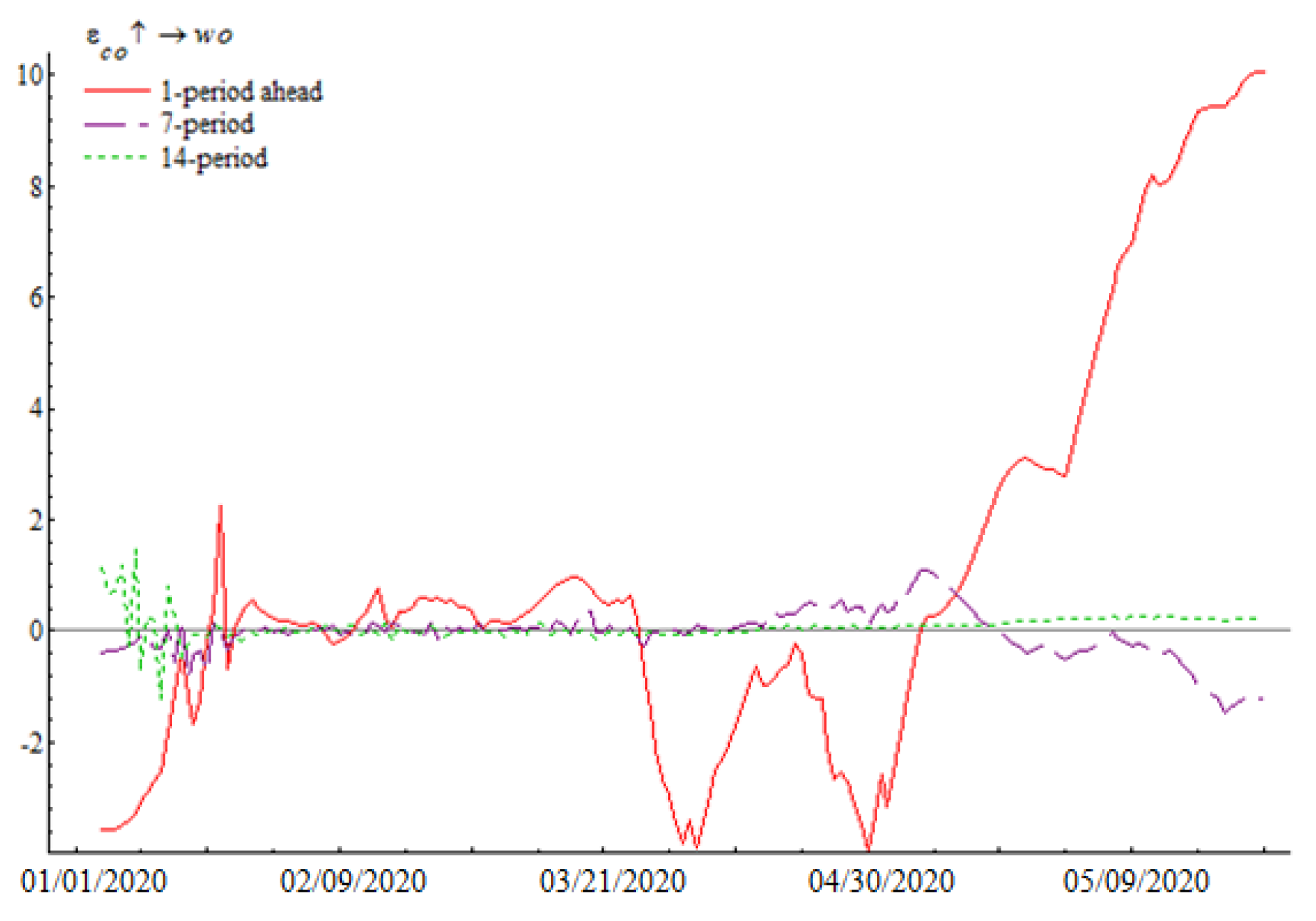
Figure 4 shows the final dynamic relationship between the COVID-19 pandemic and China’s log prices. Initially, the impulse response of the growth rate of log prices to the changes in the number of people diagnosed with COVID-19 in mainland China was descending. The impulse response fluctuated around zero from the end of January to mid-March. The trough appeared at the end of March and the beginning of April and then began to rise. Since the beginning of May, it turned out to be a positive value. Furthermore, the final degree of ascending influence continued to increase in fluctuations. This result shows that initially, the impulse response of the growth rate of log prices to the changes in the number of people diagnosed with COVID-19 in mainland China was descending. The impulse response fluctuated around zero from the end of January to mid-March. The trough appeared at the end of March and the beginning of April and then began to rise. Since the beginning of May, it turned out to be a positive value. Moreover, the final degree of ascending influence continued to increase in fluctuations. This result shows that in the early phase, the number of COVID-19 confirmed cases in China would curb the growth of log prices. At that time, because of the Spring Festival, the demand for log decreased, and the price of log decreased slightly. In order to contain the spread in Wuhan, authorities imposed unprecedented restrictions on travel and ordered the closure of most businesses in the bustling metropolis and gradually stopped production around the whole country. The demand for log materials dropped sharply and evenly to zero. Thus, the price of log further decreased. Therefore, at the beginning of the first outbreak, as the pandemic worsened, the number of confirmed COVID-19 cases in mainland China increased, and log prices declined. Since it was the long holiday from the end of January to March, enterprises did not yet reopen, and there were few transactions in the wood market. Wood companies had some log stocks to produce. Therefore, the overall impact of the COVID-19 on log prices was relatively small at the beginning of 2020. In April, China’s wood processing plants gradually got back to work. However, since the COVID-19 pandemic had not been entirely over, market consumption capacity did not yet recover, and the demand was insufficient, thus log prices fell again. In May and June, due to the Suifenhe incident and the Xinfadi incident, the COVID-19 pandemic repeated, and uncertainty increased again. The simulation results show that the response of log prices did not show a trend of convergence, but turned to a positive value. It is because, since May, incidents such as overseas imports from Suifenhe and the Xinfadi Market occurred, and the COVID-19 repeated. In addition, the peak of the impulse response to log prices during the second outbreak was much more significant than during the first. The impulse response of log prices was −2.5 in January, and it reached 10 in June. It shows that the pandemic hindered upstream lumber logging, meanwhile, the consumption of downstream lumber industries such as real estate, construction, and wooden furniture has not yet recovered.
Ensuring the balance of supply and demand in the market is essential to maintain the stability of log prices. In the early phase, the pandemic caused a decline in log prices since it suppressed consumption. Meanwhile, its ascending impact on oil prices and the exchange rate and descending impact on supply caused log prices to rise. In the later period, the price of log rose due to the ascending impact of the pandemic on the exchange rate and consumption, and the descending impact on the supply, meanwhile, the price of log fell due to the ascending impact of the pandemic on the international oil prices. In conclusion, the overall results show that log prices presented an impulse response from descending to ascending to the pandemic shock. Therefore, in the early phase, demand was the main factor that affected the impact of the pandemic on log prices. In the late phase, affecting supply, demand, and the exchange rate was the dominant way to influence the impact of the pandemic on log prices.
4.4. Impulse Analysis of Different Phases
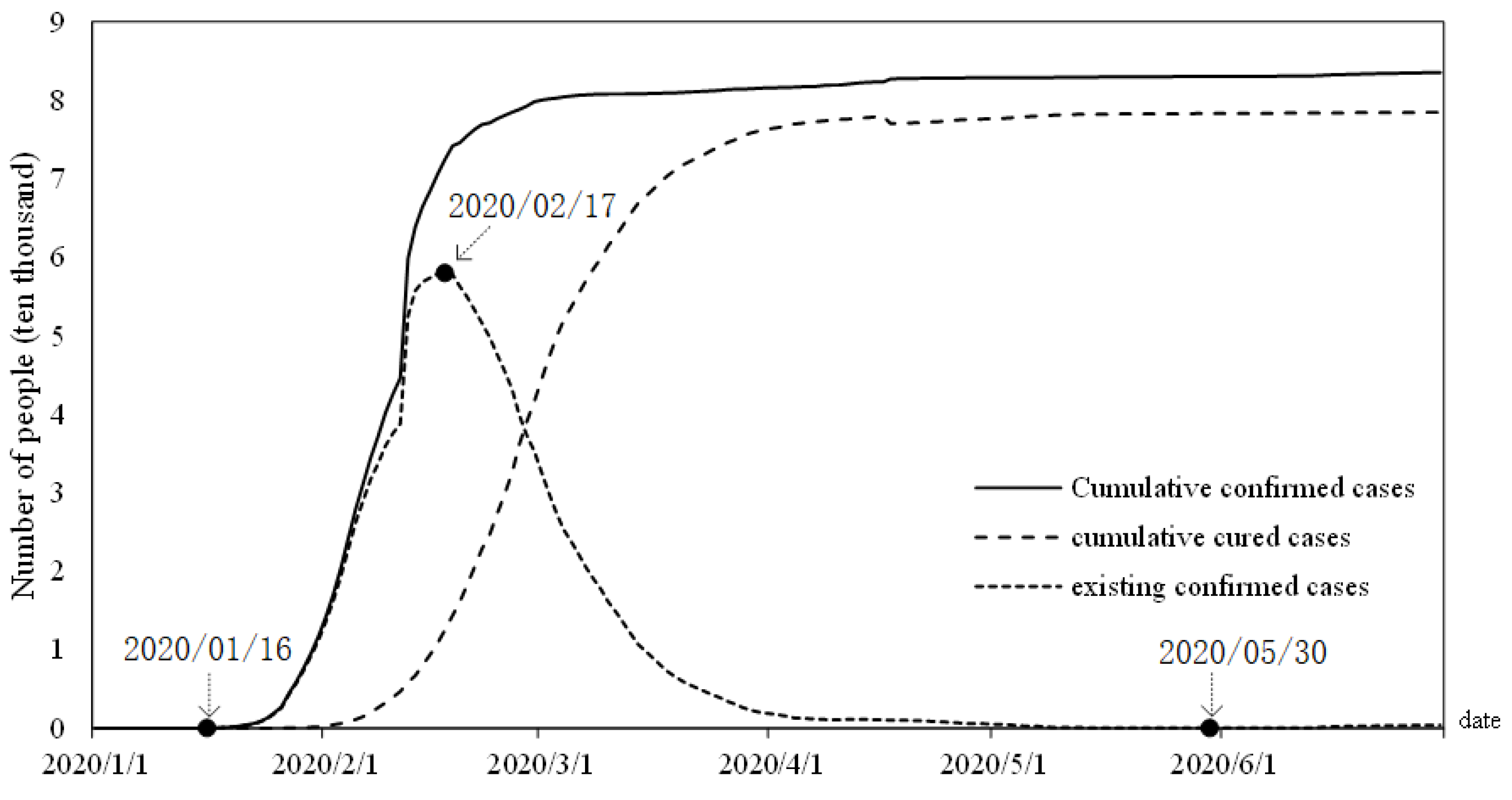
Based on the above analysis, the impact of COVID-19 on log price has obvious time-varying characteristics, which may be due to differences in the people’s expectation on the outcome of the pandemic in different time points. Therefore, this chapter uses impulse response of different points to analyze the differences in the relationship among COVID-19, international crude oil price, exchange rate, and log prices under different backgrounds. The comparison time points are 16 January, 17 February, and 30 May 2020, as in different stages of the COVID-19 pandemic (Figure 5).
Figure 5 shows that 16 January 2020 was the initial outbreak period of the pandemic. On 17 February, the number of confirmed cases of COVID-19 in mainland China reached 58,016, which was a turning point in the development of the pandemic in China. On 30 May, the pandemic was stable, but there were still some dangers, such as imported cases from abroad.
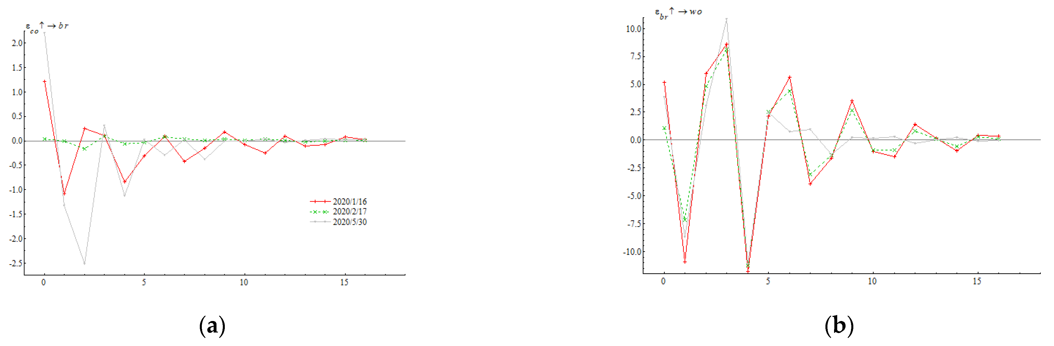
The responses of international oil prices to the COVID-19 pandemic shock at three different points were not wholly consistent. All were first reduced to the smallest negative value and then tended towards zero in the fluctuation, but the fluctuation ranges of the three were different. It can be seen in Figure 6a that the absolute value of the impulse response on 17 February 2020, was small, and the impulse response on 16 January and 30 May was massive. It might be because, on 17 February 2020, Wuhan was implementing the travel ban, many provinces and cities in China successively were also implementing social distancing policies to cope with the development of the pandemic. Since the opportunity of trade was low, the impulse response of international oil prices to the pandemic was relatively small. At the same time, the impulse responses of log prices to the oil prices shock at three different time points were consistent, and the response value fluctuated between −10 and 10 and then converges to zero. Therefore, the relationships between the pandemic and oil prices, and between international oil prices and log prices were relatively stable, and the research results were robust.
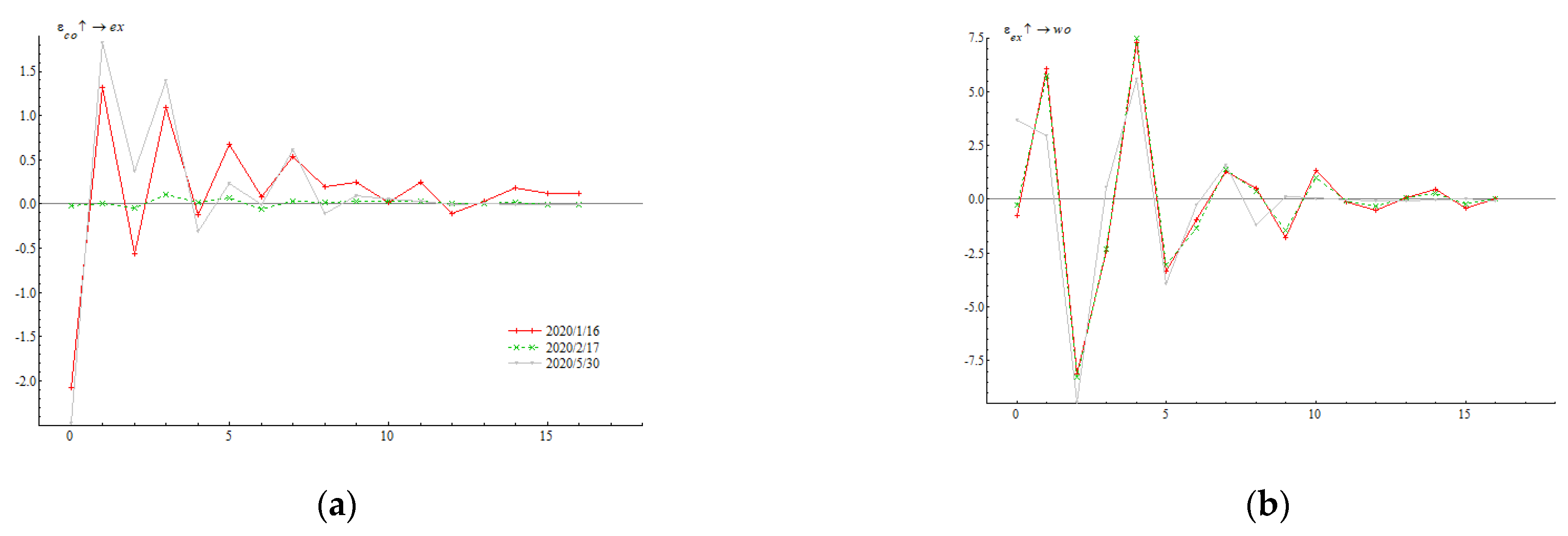
Figure 7a shows that shocks were imposed on COVID-19 at different three points. The changing trends of the impulse response function of the exchange rate to COVID-19 pandemic on 16 January and 30 May were basically similar, and both increased to the maximum value and then gradually decreased. While the exchange rate on 17 February was less affected by the COVID-19 shock. The reason may be that on 16 January, the pandemic was an emergency, with considerable uncertainty and lack of confidence in China’s market, so the exchange rate’s impulse response decreased in fluctuations. Due to the sudden increase in imported coronavirus cases from abroad on 30 May, the uncertainty also increased, which once again affected the exchange rate. On 17 February, the current number of confirmed cases of coronavirus reached the turning point, suggesting the situation was brought under control, and market confidence was then restored. Thus, at that time, the pandemic did not cause significant changes to the exchange rate. The impulse responses of log prices to the exchange rate at three different time points were consistent (Figure 7b), and the relationship between the two was relatively stable. Log prices only responded to the exchange rate from the second period, and the response was steadily approaching zero. Therefore, the relationships between the pandemic and the exchange rate and the exchange rate and log prices were relatively stable, and the research results were robust.
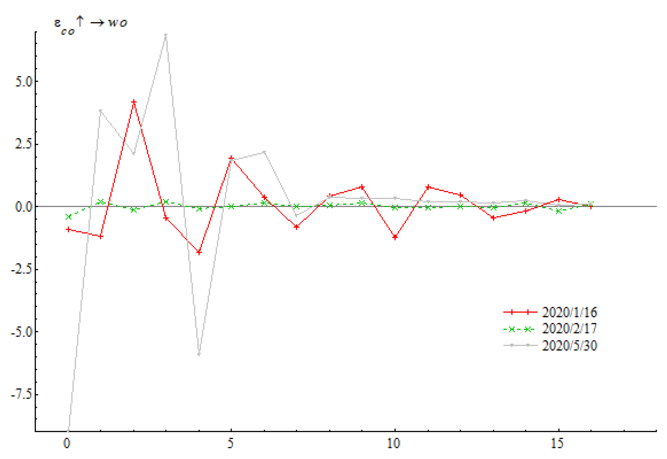
There were differences in the magnitude of the response of log prices to the new confirmed cases of COVID-19 shock at three different points because the three points were at different stages of the pandemic and faced different social conditions (Figure 8). On 16 January 2020, the early stage of the pandemic, the response of log prices to the pandemic was unstable. It was because everyone did not know enough about this disease at that time, so the impact was continually fluctuating. On 17 February 2020, the day of the turning point of the number of confirmed cases of COVID-19, the pandemic had little impact on the changes in market confidence since the pandemic got under control. Therefore, the pandemic also had little influence on consumers’ and suppliers’ decision-making, and the impulse response of log prices to the pandemic tended to be zero. On 30 May, log prices were more sensitive to the pandemic, and except for the fourth period, the impulse response gradually weakened from a positive value to zero in the fluctuation.
5. Discussion
The impact of the COVID-19 on crude oil prices is basically synchronized with the trend of the pandemic. In the wake of the coronavirus outbreak, the pandemic’s emergence led to a drop in international oil prices. After March, the impact of the pandemic had an ascending effect on crude oil prices. The pandemic in June briefly caused a drop in international oil prices, and then quickly recovered. The impact of the pandemic on log prices through oil prices was reduced, while our result is not entirely consistent with the findings of studies that Albulescu [2], Bakas and Triantafyllou [3], and Baumeister and Peersman [52] found who claim that some pandemic diseases were decreasingly correlated with international oil prices. It is because these articles did not consider the time-varying relationship between variables. We found that when the second outbreak was under control in the late June, the impulse response converged rapidly, which was significantly faster than the convergence rate of the impulse response at the beginning of the year. It shows that the response policy of the pandemic in June was more conducive to the resumption of work in the crude oil industry. We also found that the impulse response of log prices to international oil prices was always descending. That is, the ascending impact of oil prices would not lead to an increase in log prices. It is inconsistent with Hypothesis 1. It might be because, after the first outbreak, a large number of oil refineries and petrochemical companies suspended production. Although the international crude oil prices fell sharply, the crude oil could not be refined and processed in time. The changes in international crude oil prices could not be immediately mapped to fuel oil prices and transportation costs, which led to a hysteresis. Furthermore, international crude oil prices affected log prices by changing transportation costs. Influenced by the pandemic, shipping voyages decreased, while transportation time and capital cost increased. International oil prices might no longer be the main reason affecting transportation costs. Therefore, oil prices fell due to the impact of the COVID-19 in the early phase, but the price of log rose. In the late phase, oil prices re-covered somewhat, but the pandemic caused a decline in log prices through international oil prices. In June, it became shortly ascending. It illustrates that control measures are more effective in June compared with the beginning of the outbreak.
The impact of the pandemic on the exchange rate is also similar to the trend of the pandemic. In the early phase of 2020, first of all, the sudden outbreak of COVID-19 caused emotional fluctuations in the market. If the pandemic could not be adequately controlled, it might affect the development of China’s economy. Insufficient confidence in the Chinese market contributed to the outflowing of foreign exchange, which then led to currency depreciation. While China’s wood consumption was more dependent on imports, the above process might increase the price of log in RMB. Second, COVID-19 is a public health emergency of international concern, which caused losses to China’s export trade and reduced foreign exchange inflows. It might cause the RMB’s devaluation, which in turn would increase the price of log RMB. In addition, the RMB is an emerging market currency. When global risk aversion is on the rise, international investors may consider selling Chinese assets, which may cause capital outflows. RMB’s devaluation pressure would increase, which may eventually increase the price in RMB of log. As time goes by, the pandemic in China was gradually brought under control due to the decisive government intervention, China’s economy and financial markets gradually recovered, and the market confidence was boosted again. At the same time, international pandemic prevention and control measures were not strict, resulting in a problematic global pandemic situation. Although China’s economy recovered, international economic growth stalled. In the end, compared with China and other countries, the impact of the pandemic on the exchange rate gradually weakened, and the impact of the pandemic on the increase in log prices through the exchange rate also weakened. With the control of the pandemic at the beginning of 2020, the impulse response converged, and the speed was consistent with the changes in the pandemic. It shows that as long as the pandemic is under control, the exchange rate has a chance to recover. However, in May and June, due to the Suifenhe incident and the “salmon incident” in the Beijing Xinfadi Market caused by cases of overseas imports, the number of newly diagnosed patients increased, and market uncertainty suddenly increased. Then, the second COVID-19 outbreak appeared. The ascending impulse response of the pandemic on the exchange rate suddenly increased, and the impact on log prices also increased again. After the control measures of the second outbreak was issued, the impulse response quickly converged, which was similar to the decrease in the number of newly diagnosed cases of COVID-19. It also demonstrates that the control measures of the outbreaks are conducive to the stability of the exchange rate.
The impact of the pandemic on log prices is not entirely consistent with the trend of the pandemic. During the first coronavirus outbreak, taking all the factors into consideration, the pandemic reduced the price of log. From January to March, the pandemic had little effect on domestic log prices and caused a decline in log prices in March and April. In May, the impact of the pandemic caused log prices to rise. Compared with the first quarter in 2020, the current number of confirmed cases increased at a slower rate in May and June. Residents’ ability to consume wooden furniture and paper products went up, and domestic demand for wood raw materials also rose. After China completely stopped commercial logging of natural forests in 2017, China’s commercial wood output decreased by about 40 million cubic meters each year, making it challenging to meet China’s market demand. Imported lumber was used to make up for the shortage of raw materials from then on. Due to the deterioration of the world pandemic, the industrial chains in some major wood supply counties such as the USA and Canada were interrupted. Meanwhile, the pressure of imported cases from abroad continued to increase, and shipping companies reduced their schedules, which brought significant obstacles to the international trade of wood raw materials. Therefore, in May and June, the impact of the pandemic on log prices increased rapidly, and we could not see a trend of convergence until 30 June. As market regulation requires response time, although the pandemic is effectively controlled in China, the impact of the pandemic on log prices is still getting stronger. It shows that COVID-19 has a long-term impact on the wood industry. In addition, since China’s wood industry aims to export-led growth and the economy of the world is sluggish, the resumption of production of China’s wood industry is not smooth. Therefore, it is necessary to promote the development of the domestic wood market and realize the “dual circulation” of China’s wood industry. The “Dual circulation” strategy was first mentioned in May 2020. The strategy aims to gradually form a new development model in which domestic circulation plays a dominant role meanwhile pay attention to external circulation (export-oriented development). “Dual circulation” in the wood industry means to take China’s wood market as the mainstay while making both internal and external wood markets promote each other.
6. Conclusions
In order to compare the impact of the COVID-19 pandemic on log prices in different periods and explore the speed of log prices recovery under different control measures, this paper uses the TVP-VAR model to conduct an empirical study on the dynamic transmission effect of the coronavirus pandemic on log prices. The results show that COVID-19, directly and indirectly, affected log prices. First, the pandemic indirectly affected log prices by changing international oil prices and the exchange rate. We found that the impact of the pandemic on oil prices and exchange rates is synchronized with changes in the severity of COVID-19 and is predominantly in the short-term. As the pandemic eased, the impact of the pandemic on crude oil prices and the exchange rate reduced. However, as for log prices, after the pandemic eased in June, the impact of the pandemic on log prices did not diminish while remaining increasing. Third, comparing the impulse response of crude oil prices and the exchange rate in the first and second outbreaks, they had the same response direction and similar magnitude, but the impulse response in June converges faster. Thus, control measures in June are more effective comparing with the beginning of 2020. The peak value of the impulse response of log prices to the second outbreak was greater than the first. It shows that the COVID-19 pandemic has a long-term influence on the wood industry in China, and the resumption of business in China’s wood industry is not smooth. Therefore, it is necessary to solve the imbalance between supply and demand as soon as possible. Last but not least, in the early stage, the demand market was dominant in the process of the pandemic’s impact on log prices. In the late phase, the pandemic mainly changed the log prices by affecting supply, demand, and the exchange rate. Therefore, ensuring the balance of supply and demand in the market is an essential means to maintain the stability of log prices at this moment. As a result, the process of COVID-19 impacting log prices during the first half of 2020 provides evidence-based strategies that could be used as a reference if the pandemic becomes a “new normal”. Moreover, these could also be some general lessons that other countries might learn from existing evidence in terms of the safe development of the wood industry.
Based on the above research conclusions and the status quo of China’s wood industry, this paper proposes implications for China’s wood industry:
First, learn from the partial quarantine policy in June. We find that control measures were more effective in June compared with the beginning of 2020. Thus, if the pandemic becomes a “new normal”, we should refer to the prevention and control measures taken in June and formulate new response strategies. Second, speed up the plantation cultivation and increase domestic lumber supply. As an emergency, the COVID-19 pandemic blocked lumber import channels causing insufficient log supply, which acts as the main reason for unstable log prices. As the raw material for the wood products industry, rising log prices seriously affect the production cost of products and ultimately cause more significant losses to the wood industry. The authorities should introduce reasonable industrial policies to take advantage of the current rising log prices to strengthen forest farmers’ enthusiasm for growing lumber. The Chinese government should coordinate the cultivation and production of domestic lumber raw materials, gradually increase wood supply to meet domestic wood demand, thereby decreasing the industry’s dependence on external wood materials, and reducing the fluctuations in China’s wood prices caused by uncertain factors in the international trade. The leadership should promote a “dual circulation” development pattern centered on the domestic economy, and aimed at integrating the domestic and international economies to fundamentally realize China’s wood safety.
Author Contributions
Conceptualization, B.C. and C.T.; methodology, C.T.; software, C.T. and G.D.; validation, G.D.; formal analysis, B.C. and G.D.; investigation, C.T.; resources, C.T.; data curation, C.T.; writing—original draft preparation, C.T.; writing—review and editing, B.C. and G.D.; visualization, B.C.; supervision, B.C.; project administration, B.C.; funding acquisition, B.C. All authors have read and agreed to the published version of the manuscript.
Funding
This research was funded by the National Natural Science Foundation of China, grant number 71873016.
Data Availability Statement
All data used during the study are available from the corresponding author by request.
Acknowledgments
We would like to highly thank Kent Wheiler at the University of Washington for extensive English revision. We also thank the China Scholarship Council (CSC) for the financial support (CSC no. 201906510035). We also really appreciate the comments that the editors and reviewers have provided.
Conflicts of Interest
The authors declare no conflict of interest.
References
- Zhu, T.; Zhao, Q.; Yang, H.; Ding, S. Influence of carbon sink value on China’s wood price based on VAR model. J. Nanjing For. Univ. (Natl. Sci. Ed.) 2018, 42, 191–195. (In Chinese) [Google Scholar] [CrossRef]
- Albulescu, C. Coronavirus and oil price crash. SSRN Electron. J. 2020. [Google Scholar] [CrossRef]
- Bakas, D.; Triantafyllou, A. Commodity price volatility and the economic uncertainty of pandemics. Econ. Lett. 2020, 109283. [Google Scholar] [CrossRef]
- Reportlinker. Wood Processing Global Market Report 2021: COVID 19 Impact and Recovery to 2030, 17 February 2021. Available online: https://www.reportlinker.com/p06025306/Wood-Processing-Global-Market-Report-COVID-19-Impact-and-Recovery-to.html?utm_source=GNW (accessed on 13 March 2021).
- Southern Forest Products Association. How will COVID19 Affect China’s Timber Industry? 25 March 2020. Available online: http://sfpa.org/wp-content/uploads/2020/03/COVID19s-impact-to-China-timber-industry-1.pdf (accessed on 13 March 2021).
- Global Wood Markets Info. Analysis: What’s the impact Of the Coronavirus on the Chinese Timber Industry? 20 March 2020. Available online: https://www.globalwoodmarketsinfo.com/forecast-whats-the-impact-of-the-coronavirus-on-the-chinese-timber-industry/ (accessed on 13 March 2021).
- Hart, C.E.; Hayes, D.J.; Jacobs, K.L.; Schulz, L.L.; Crespi, J.M. The Impact of COVID-19 on Iowa’s Corn, Soybean, Ethanol, Pork, and Beef Sectors. Center for Agricultural and Rural Development, Iowa State University. 2020. Available online: https://econpapers.repec.org/paper/iascpaper/20-pb28.htm (accessed on 11 December 2020).
- Brewin, D.G. The impact of COVID-19 on the grains and oilseeds sector. Can. J. Agric. Econ. Rev. Can. D’Agroecon. 2020, 68, 185–188. [Google Scholar] [CrossRef] [Green Version]
- Xu, G.; Li, Z. The Impact of COVID-19 Epidemic on China’s Mask Industry. Rev. Econ. Manag. 2020, 36, 11–20. (In Chinese) [Google Scholar] [CrossRef]
- Del Rio-Chanona, R.M.; Mealy, P.; Pichler, A.; Lafond, F.; Farmer, J.D. Supply and demand shocks in the COVID-19 pandemic: An industry and occupation perspective. Covid Econ. 2020, 6, 65–103. [Google Scholar] [CrossRef]
- Laing, T. The economic impact of the Coronavirus 2019 (Covid-2019): Implications for the mining industry. Extr. Ind. Soc. 2020, 7, 580–582. [Google Scholar] [CrossRef] [PubMed]
- Fernandes, N. Economic Effects of Coronavirus Outbreak (COVID-19) on the World Economy. Available online: https://papers.ssrn.com/sol3/papers.cfm?abstract_id=3557504 (accessed on 23 March 2020).
- Bakar, N.A.; Rosbi, S. Effect of Coronavirus disease (COVID-19) to tourism industry. Int. J. Adv. Eng. Res. Sci. 2020, 7, 189–193. [Google Scholar] [CrossRef] [Green Version]
- Simões, D.; Andrés Daniluk Mosquera, G.; Cristina Batistela, G.; Raimundo de Souza Passos, J.; Torres Fenner, P. Quantitative analysis of uncertainty in financial risk assessment of road transportation of wood in Uruguay. Forests 2016, 7, 130. [Google Scholar] [CrossRef] [Green Version]
- Frisk, M.; Göthe-Lundgren, M.; Jörnsten, K.; Rönnqvist, M. Cost allocation in collaborative forest transportation. Eur. J. Oper. Res. 2010, 205, 448–458. [Google Scholar] [CrossRef] [Green Version]
- Hejazian, M.; Lotfalian, M.; Lindroos, O.; Mohammadi Limaei, S. Wood transportation machine replacement using goal programming. Scand. J. For. Res. 2019, 34, 635–642. [Google Scholar] [CrossRef]
- Daigneault, A.J.; Sohngen, B.; Sedjo, R. Exchange rates and the competitiveness of the United States timber sector in a global economy. For. Policy Econ. 2008, 10, 108–116. [Google Scholar] [CrossRef]
- Israel, D.C.; Bunao, D.F.M. Value Chain Analysis of the Wood Processing Industry in The Philippines. PIDS Discussion Paper Series. 2017. Available online: http://hdl.handle.net/10419/173582 (accessed on 2 March 2020).
- Kaputa, V.; Paluš, H.; Vlosky, R. Barriers for wood processing companies to enter foreign markets: A case study in Slovakia. Eur. J. Wood Wood Prod. 2016, 74, 109–122. [Google Scholar] [CrossRef]
- Hosseini, M.; Brege, S.; Nord, T. A combined focused industry and company size investigation of the internationalization-performance relationship: The case of small and medium-sized enterprises (SMEs) within the Swedish wood manufacturing industry. For. Policy Econ. 2018, 97, 110–121. [Google Scholar] [CrossRef]
- Shrabana Mukherjee. Wood Industry Outlook Hit by Low Lumber Prices, Soft Housing, 22 August 2019. Available online: https://www.zacks.com/commentary/482441/wood-industry-outlook-hit-by-low-lumber-prices-soft-housing (accessed on 14 March 2021).
- National Forestry and Grassland Administration. The impact of the new crown epidemic on China’s timber industry and its analysis report, 26 April 2020. Available online: http://www.forestry.gov.cn/xdly/5188/20200426/094914870594585.html (accessed on 25 August 2020).
- Bollen, K.A. Total, direct, and indirect effects in structural equation models. Sociol. Methodol. 1987, 17, 37–69. [Google Scholar] [CrossRef] [Green Version]
- Conrad, I.V.; Joseph, L. Costs and challenges of log truck transportation in Georgia, USA. Forests 2018, 9, 650. [Google Scholar] [CrossRef] [Green Version]
- Jayaraman, T.K.; Choong, C.K. Growth and oil price: A study of causal relationships in small Pacific Island countries. Energy Policy 2009, 37, 2182–2189. [Google Scholar] [CrossRef]
- Feng, X.; Wang, Y.; Liu, S.; Jia, W.; Yang, X. Impacts of COVID-19 on Urban Rail Transit Operation. Transp. Res. 2020, 6, 45–49. (In Chinese). [Google Scholar]
- Solaymani, S.; Kardooni, R.; Kari, F.; Yusoff, S.B. Economic and environmental impacts of energy subsidy reform and oil price shock on the Malaysian transport sector. Travel Behav. Soc. 2015, 2, 65–77. [Google Scholar] [CrossRef]
- Cook, J.A. The effect of firm-level productivity on exchange rate pass-through. Econ. Lett. 2014, 122, 27–30. [Google Scholar] [CrossRef] [Green Version]
- Seth, H.; Talwar, S.; Bhatia, A.; Saxena, A.; Dhir, A. Consumer resistance and inertia of retail investors: Development of the resistance adoption inertia continuance (RAIC) framework. J. Retail. Consum. Serv. 2020, 55, 102071. [Google Scholar] [CrossRef]
- Zhang, D.; Hu, M.; Ji, Q. Financial markets under the global pandemic of COVID-19. Financ. Res. Lett. 2020, 36, 101528. [Google Scholar] [CrossRef] [PubMed]
- Elbadawi, I.A.; Soto, R. Real exchange rates and macroeconomic adjustments in sub-Saharan Africa and other developing countries. J. Afr. Econ. 1997, 74–120. [Google Scholar] [CrossRef]
- Combes, J.L.; Kinda, T.; Plane, P. Capital flows, exchange rate flexibility, and the real exchange rate. J. Macroecon. 2012, 34, 1034–1043. [Google Scholar] [CrossRef] [Green Version]
- Haim, D.; Adams, D.M.; White, E.M. Determinants of demand for wood products in the US construction sector: An econometric analysis of a system of demand equations. Can. J. For. Res. 2014, 44, 1217–1226. [Google Scholar] [CrossRef]
- Schlosser, W.E. Real price appreciation forecast tool: Two delivered log market price cycles in the Puget Sound markets of western Washington, USA, from 1992 through 2019. For. Policy Econ. 2020, 113, 102114. [Google Scholar] [CrossRef]
- Zeng, H.; Su, L.; Tan, Y. The Heterogeneous Impact of Media Negative Coverage of Agricultural Product Safety on the Price Fluctuations of Agricultural Product. J. Agrotech. Econ. 2019, 8, 99–114. (In Chinese) [Google Scholar] [CrossRef]
- Buongiorno, J.; Johnston, C. Potential effects of US protectionism and trade wars on the global forest sector. For. Sci. 2018, 64, 121–128. [Google Scholar] [CrossRef] [Green Version]
- Wu, L.; Fu, G. RMB exchange rate, short-turn capital flows and stock price. Econ. Res. J. 2014, 49, 72–86. (In Chinese) [Google Scholar]
- Nakajima, J.; Kasuya, M.; Watanabe, T. Bayesian analysis of time-varying parameter vector autoregressive model for the Japanese economy and monetary policy. J. Jpn. Int. Econ. 2011, 25, 225–245. [Google Scholar] [CrossRef] [Green Version]
- Primiceri, G.E. Time varying structural vector autoregressions and monetary policy. Rev. Econ. Stud. 2005, 72, 821–852. [Google Scholar] [CrossRef]
- Zhou, J. The Research on Third-Party Logistics Services Provider Selection for Timber Importing. Ph.D. Thesis, Central South University of Forestry and Technology, Changsha, China, 2019. (In Chinese). [Google Scholar]
- Luft, G. The Oil Crisis and its Impact on the Air Cargo Industry. Institute for the Analysis of Global Security. 2006. Available online: http://www.iags.org/aircargo406.pdf (accessed on 2 March 2020).
- Yilmazkuday, H. Oil Shocks through International Transport Costs, Evidence from U.S. Business Cycles Federal Reserve Bank of Dallas. Globalization and Monetary Policy Institute, Working Paper, 2011, p. 82. Available online: http://www.dallasfed.org/institute/wpapers/2011/0082.pdf (accessed on 2 March 2020).
- Tran, N.K.; Haasis, H.D. An empirical study of fleet expansion and growth of ship size in container liner shipping. Int. J. Prod. Econ. 2015, 159, 241–253. [Google Scholar] [CrossRef]
- Peng, H.; Zhu, X. Multiple Arbitrage Motives and Shock Effects of Short-term Capital Flows: Dynamic Analysis Based on TVP-VAR. Econ. Res. J. 2019, 54, 36–52. (In Chinese) [Google Scholar]
- Mehrotra, S.N.; Carter, D.R. Forecasting performance of lumber futures prices. Econ. Res. Int. 2017, 2017, 1–8. [Google Scholar] [CrossRef] [Green Version]
- Chudy, R.P.; Hagler, R.W. Dynamics of global roundwood prices–Cointegration analysis. For. Policy Econ. 2020, 115, 102155. [Google Scholar] [CrossRef]
- Reimer, J.J. An investigation of log prices in the US Pacific Northwest. For. Policy Econ. 2021, 126, 102437. [Google Scholar] [CrossRef]
- Kożuch, A.; Banaś, J. The Dynamics of Beech Roundwood Prices in Selected Central European Markets. Forests 2020, 11, 902. [Google Scholar] [CrossRef]
- Toppinen, A.; Viitanen, J.; Leskinen, P.; Toivonen, R. Dynamics of roundwood prices in Estonia, Finland and Lithuania. Baltic For. 2005, 11, 88–96. [Google Scholar]
- Schwert, G.W. Tests for unit roots: A Monte Carlo investigation. J. Bus. Econ. Stat. 2002, 20, 5–17. [Google Scholar] [CrossRef]
- Lütkepohl, H. New Introduction to Multiple Time Series Analysis; Springer: Berlin/Heidelberg, Germany, 2005; pp. 135–156. [Google Scholar]
- Baumeister, C.; Peersman, G. The Role of Time-Varying Price Elasticities in Accounting for Volatility Changes in the Crude Oil Market. J. Appl. Econom. 2013, 28, 1087–1109. [Google Scholar] [CrossRef] [Green Version]
Figure 1.
Estimation results of the time-varying parameter (TVP) regression model for the simulated data.
Figure 1.
Estimation results of the time-varying parameter (TVP) regression model for the simulated data.

Figure 2.
Impulse responses for the set COVID-19, international oil prices, and log prices. Note: The abscissa refers to the date in the first half of 2020, and the ordinate indicates the impulse response values after the shock of one-unit standard deviation. The figure shows the impulse response of oil prices to the pandemic (a) and the impulse response of log prices to oil prices (b).

Figure 3.
Impulse responses for the set COVID-19, exchange rate, and log prices. Note: The abscissa refers to the date in the first half of 2020, and the ordinate indicates the impulse response values after the shock of one-unit standard deviation. The figure shows the impulse response of exchange rate to the pandemic (a) and the impulse response of log prices to exchange rate (b).

Figure 4.
Impulse responses for the set COVID-19 and log prices. Note: The abscissa refers to the date in the first half of 2020, and the ordinate indicates the impulse response values after the shock of one-unit standard deviation.
Figure 4.
Impulse responses for the set COVID-19 and log prices. Note: The abscissa refers to the date in the first half of 2020, and the ordinate indicates the impulse response values after the shock of one-unit standard deviation.

Figure 5.
Trends of COVID-19 in China from January to June 2020. Data source: National Health Commission of the People’s Republic of China.
Figure 5.
Trends of COVID-19 in China from January to June 2020. Data source: National Health Commission of the People’s Republic of China.

Figure 6.
Impulse responses at different points for the set COVID-19, oil prices, and log prices. Note: The abscissa refers to the number of lag periods of the impact, and the ordinate indicates the impulse response values after the shock of one-unit standard deviation. The figure shows the impulse response of oil prices to the pandemic (a) and the impulse response of log prices to oil prices (b) at different points.

Figure 7.
Impulse responses at different points for the set COVID-19, exchange rate, and log prices. Note: The abscissa refers to the number of lag periods of the impact, and the ordinate indicates the impulse response values after the shock of one-unit standard deviation. The figure shows the impulse response of exchange rate to the pandemic (a) and the impulse response of log prices to exchange rate (b) at different points.

Figure 8.
Impulse responses at different points for the set COVID-19 and log prices. Note: The abscissa refers to the number of lag periods of the impact, and the ordinate indicates the impulse response values after the shock of one-unit standard deviation.
Figure 8.
Impulse responses at different points for the set COVID-19 and log prices. Note: The abscissa refers to the number of lag periods of the impact, and the ordinate indicates the impulse response values after the shock of one-unit standard deviation.


Table 1.
Augmented Dickey–Fuller test.
| Variables | Without Constant & Drift | With Drift | With Constant & Drift | Conclusions | |
|---|---|---|---|---|---|
| Original Level | CO | −1.681 * | −2.112 ** | −3.128 | non-stationarity |
| BR | −1.099 | −1.584 * | −0.789 | non-stationarity | |
| EX | 1.053 | −1.900 ** | −2.313 | non-stationarity | |
| WO | −0.125 | −2.905 *** | −3.057 | non-stationarity | |
| First-order Difference | co | −3.175 *** | −3.165 *** | −3.221 * | stationary |
| br | −3.259 *** | −3.296 *** | −3.701 ** | stationary | |
| ex | −3.927 *** | −4.096 *** | −4.232 *** | stationary | |
| wo | −3.902 *** | −3.870 *** | 3.862 ** | stationary |
Note: standard error values are in parentheses. *** p < 0.01, ** p < 0.05, * p < 0.10.
Table 2.
Estimation results of selected parameters in the time-varying parameter autoregressive (TVP-VAR) model.
Table 2.
Estimation results of selected parameters in the time-varying parameter autoregressive (TVP-VAR) model.
| Parameter. | Mean | Stdev. | 95% Percent Interterval | CD | Inefficiency |
|---|---|---|---|---|---|
| 0.0229 | 0.0026 | (0.0185, 0.0287) | 0.465 | 10.14 | |
| 0.0226 | 0.0026 | (0.0181, 0.0282) | 0.452 | 6.17 | |
| 0.0564 | 0.0173 | (0.0345, 0.0961) | 0.540 | 29.22 | |
| 0.0701 | 0.0327 | (0.0345, 0.1552) | 0.223 | 39.31 | |
| 0.9326 | 0.1340 | (0.6995, 1.2247) | 0.611 | 26.12 | |
| 0.7727 | 0.1209 | (0.5603, 1.0241) | 0.239 | 78.58 |
Publisher’s Note: MDPI stays neutral with regard to jurisdictional claims in published maps and institutional affiliations. |
© 2021 by the authors. Licensee MDPI, Basel, Switzerland. This article is an open access article distributed under the terms and conditions of the Creative Commons Attribution (CC BY) license (https://creativecommons.org/licenses/by/4.0/).
Share and Cite
MDPI and ACS Style
Tao, C.; Diao, G.; Cheng, B. The Dynamic Impacts of the COVID-19 Pandemic on Log Prices in China: An Analysis Based on the TVP-VAR Model. Forests 2021, 12, 449. https://doi.org/10.3390/f12040449
AMA Style
Tao C, Diao G, Cheng B. The Dynamic Impacts of the COVID-19 Pandemic on Log Prices in China: An Analysis Based on the TVP-VAR Model. Forests. 2021; 12(4):449. https://doi.org/10.3390/f12040449
Chicago/Turabian StyleTao, Chenlu, Gang Diao, and Baodong Cheng. 2021. "The Dynamic Impacts of the COVID-19 Pandemic on Log Prices in China: An Analysis Based on the TVP-VAR Model" Forests 12, no. 4: 449. https://doi.org/10.3390/f12040449
Note that from the first issue of 2016, this journal uses article numbers instead of page numbers. See further details here.