MaxEnt Modeling Based on CMIP6 Models to Project Potential Suitable Zones for Cunninghamia lanceolata in China
by
 , , ,
, , ,
Yichen Zhou
1 ,
,
Zengxin Zhang
1,2,*,
Bin Zhu
1,
Xuefei Cheng
1,
Liu Yang
1,
Mingkun Gao
1 and
Rui Kong
2 1
Co-Innovation Center for Sustainable Forestry in Southern China, Jiangsu Province Key Laboratory of Soil and Water Conservation and Ecological Restoration, Nanjing Forestry University, 159 Longpan Road, Nanjing 210037, China
2
State Key Laboratory of Hydrology-Water Resources and Hydraulics Engineering, Hohai University, Nanjing 210098, China
*
Author to whom correspondence should be addressed.
Forests 2021, 12(6), 752; https://doi.org/10.3390/f12060752
Submission received: 18 May 2021
/
Revised: 1 June 2021
/
Accepted: 4 June 2021
/
Published: 7 June 2021
(This article belongs to the Section Forest Inventory, Modeling and Remote Sensing)
Abstract
:Cunninghamia lanceolata (Lamb.) Hook. (Chinese fir) is one of the main timber species in Southern China, which has a wide planting range that accounts for 25% of the overall afforested area. Moreover, it plays a critical role in soil and water conservation; however, its suitability is subject to climate change. For this study, the appropriate distribution area of C. lanceolata was analyzed using the MaxEnt model based on CMIP6 data, spanning 2041–2060. The results revealed that (1) the minimum temperature of the coldest month (bio6), and the mean diurnal range (bio2) were the most important environmental variables that affected the distribution of C. lanceolata; (2) the currently suitable areas of C. lanceolata were primarily distributed along the southern coastal areas of China, of which 55% were moderately so, while only 18% were highly suitable; (3) the projected suitable area of C. lanceolata would likely expand based on the BCC-CSM2-MR, CanESM5, and MRI-ESM2-0 under different SSPs spanning 2041–2060. The increased area estimated for the future ranged from 0.18 to 0.29 million km2, where the total suitable area of C. lanceolata attained a maximum value of 2.50 million km2 under the SSP3-7.0 scenario, with a lowest value of 2.39 million km2 under the SSP5-8.5 scenario; (4) in combination with land use and farmland protection policies of China, it is estimated that more than 60% of suitable land area could be utilized for C. lanceolata planting from 2041–2060 under different SSP scenarios. Although climate change is having an increasing influence on species distribution, the deleterious impacts of anthropogenic activities cannot be ignored. In the future, further attention should be paid to the investigation of species distribution under the combined impacts of climate change and human activities.
1. Introduction
In recent years, climate change has adversely affected ecosystems and myriad biological species on a global scale [1,2,3,4]. Continuously intensifying deleterious changes in climate may lead to the extinction of nearly one-quarter of the world’s species [5,6]. To prevent these global warming-induced losses, it is critical to develop the capacity to predict the potential distribution of species under global climate change, as well as formulate long term strategies for the protection of species to ensure the sustainability of the biosphere in the future [7].
To better analyze the past, present and future of climate change, the Coupled Model Intercomparison Project (CMIP) was implemented by the Intergovernmental Panel on Climate Change (IPCC) twenty years ago. The Representative Concentration Pathways (RCPs) adopted in the fifth assessment report (AR5) of IPCC were a series of integrated concentration and emission scenarios. The global climate models (GCMs) from different phases of the CMIP have been at the heart of climate change studies [8]. RCPs each contain 4 scenarios and more than 50 models from around the world are involved, including the BCC-CSM1 model from China [9].
In 2021, the sixth phase of the Coupled Model Comparison Program (CMIP6) uses the latest climate model in which a set of new emission scenarios are driven by shared socioeconomic pathways (SSPs). The SSPs each provide five different pathways for future socioeconomic development and contain possible trends in agriculture and land use. Nearly 50 models from 14 countries participated in it [10].
Recently, species distribution models (SDMs) have been utilized to estimate species niches according to specific algorithms, through the analysis of current species occurrence data and environmental variables [11]. Subsequently, these estimations can be employed to map potentially suitable areas for specific species [12]. The main SDMs used to evolve these predictions include Domain Model [13], Ecological Niche Factor Analysis (ENFA) [14], the Bioclimatic Prediction System (Bioclim) [15], genetic algorithm for rule set production (GARP) [16], and maximum entropy models [17].
MaxEnt is a niche model based on an environmental variables layer and species distribution records, which integrates machine learning and maximum entropy principles to simulate the potential geographical distribution of species [18]. Compared with other models, the MaxEnt model performs better, due to its ability to model presence-only data [19,20], and it is thought to be robust for small sample sizes [21,22]. Furthermore, it has the capacity to model complex, non-linear relationships between response variables and predictors [23]. Due to its simplicity and ease of use, MaxEnt has become one of the best and most extensively used SDM models that can meet different research objectives [24,25,26].
Recently, many research studies have predicted the modification of potential distribution for many species affected by the climate change in the future [27]. For example, Kong et al. [28] employed the MaxEnt model to predict the likely distribution of Osmanthus fragrans (Thunb.) Lour and revealed that its central growth area would decrease and migrate to Southwest China from 2061–2080. Moreover, the lost suitable area of O. fragrans under the RCP8.5 scenario would be three times that under RCP2.6 scenario from 2061–2080. Zhang et al. [29] used the MaxEnt model to predict the distribution of Cinnamomum camphora (L.) J. Presl and reported that the increasingly rapid expansion of a suitable C. camphora range under a high greenhouse gas emission scenario would be far faster than under a lower emissions scenario spanning 2055–2085. At the end of the 21st century, the area suitable for C. camphora under RCP4.5 and RCP8.5 would increase by 84.8% and 130%, respectively, compared with today. Zhang et al. [30] found that the suitable area of Euscaphis japonica (Thunb.) Dippel would geographically expand further north in the 2050s and 2070s under the RCP2.6 scenario, as predicted by MaxEnt and GARP. However, the suitable area would increase by 2050 then decrease by 2070 under the RCP8.5 scenario. Furthermore, Li et al. [31] reported that the suitable area for C. lanceolata would become fragmentated, projected by the MaxEnt model using the BCC-CSM1-1 data under different climate change scenarios from 2041–2080.
However, predictions based on a single global climate model (GCM) were inevitably uncertain in particular extreme conditions. Besides, the latest CMIP6 showed higher accuracy statistics, particularly in terms of precipitation, and reduced errors in precipitation and temperature in contrast to CMIP5 [32], as the prediction of one single global climate model is uncertain and unable to show the trend of future climate accurately [33]. The multi-model ensemble (MME) method has become the most widely used method to reduce the uncertainty of independent models and it has been emphasized by many studies [34,35,36]. Arithmetic averaging was one of the most commonly used approaches. Arithmetic averaging was based on the notion of the ‘one-model-one vote’ model democracy, i.e., all the GCMs were integrated with the same weight in it [37,38]. The higher the number of models used in the MME, the more accurate the ensemble results [34].
In recent decades, land use/land cover change (LUCC) has become increasingly important for its possibilities to map and characterize land cover based on observation and remote sensing [39], and it has been employed to address the problem in various aspects, such as forest fragmentation [40], agricultural expansion [41,42], and suburbanization [43]. Along with a large number of forest land into farmland cases, the global forest area has decreased significantly in recent years [44].
Cunninghamia lanceolata (Lamb.) Hook. (Chinese fir) is a native species of China with a long planting history, which is widely distributed across the Yangtze River basin, as well as 16 southern provinces and autonomous regions. It is a subtropical tree species with a developed shallow lateral root system and strong regeneration capacity; C. lanceolata preferentially grows in moist, acidic, well-drained soils in partial shade; it tolerates full sun, but soils should not be allowed to dry out. This species is also known for its high level of wood quality with high yields [45]. As an important economic tree species in China, the area of C. lanceolata plantations has reached 11 million hectares, with a stock volume of 625 million cubic meters; accounting for 19.01% and 25.18% of the dominant trees in China, respectively [46].
In this study, the latest shared socioeconomic pathways (SSPs) from the CMIP6 were used to project the suitable area of C. lanceolata into the future under the changing global environment. To eliminate the influence of irrelevant variables on the result and enhance the credibility of the prediction results, the BCC-CSM2, CanESM5 and MRI-ESM2-0 GCMs were used in this paper. The projected results will be arithmetic averaged to find out the most likely changes in the suitable area of C. lanceolata in the future. Furthermore, considering the relationships between future suitable areas and current land use/land cover and agricultural policies, the prediction result would be combined with the land use/land cover change data to provide a guide for the distribution of plantations with the background of global warming.
2. Materials and Methods
2.1. Current Species Data
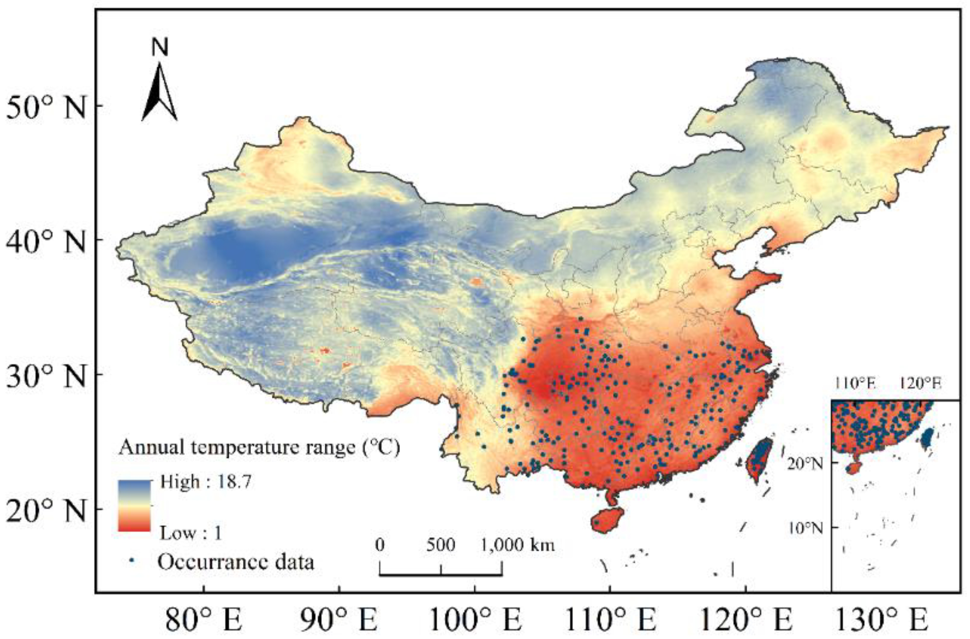
The current distribution data for C. lanceolata were collected from the Global Biodiversity Information Facility (GBIF, https//www.gbif.org, accessed on 6 December 2020) and the Chinese Virtual Herbarium (CVH, http://www.cvh.ac.cn, accessed on 6 December 2020). Any records without detailed geolocation information such as longitude or latitude, or repetitive records, were removed. A total of 406 distribution points of C. lanceolata were collected and employed to establish the MaxEnt model (Figure 1).
2.2. Environmental Variables for Model Fitting
Twenty-one variables related to the distribution of C. lanceolata were collected, including 19 bioclimatic variables (bio01–bio19) and three topographic variables (ALT, ASP, and SLO) (Table A1). This was because previous studies indicated that these environmental variables were the most significant factors for modeling potential species distribution [47]. All of the layers were at the highest spatial resolution (30 arc-second (~1 km)). The bioclimatic variables and ALT variables were obtained from the WorldClim dataset. The aspect (ASP) and slope (SLO) were extracted from the altitude by using the ArcGIS 10.5.
To avoid the influence of the multicollinearity of these variables and overfitting of the MaxEnt [48], a Pearson correlation analysis of these twenty-one variables was conducted in SPSS 22.0. When the correlation coefficient of two variables was greater than 0.80 [49], the variables with lower ecological significance were removed. The selection principle was set according to the relevant literature and the habitat of C. lanceolata [50]. Finally, 12 environmental variables (bio2, bio3, bio4, bio5, bio6, bio8, bio13, bio14, bio15, ALT, ASP, and SLO) were retained in the process in MaxEnt (Table A2).
2.3. Environmental Variables for Model Forecasting
To predict the potential distribution of C. lanceolata under future climate conditions, projections of future bioclimatic variables, according to different global climatic models and emission scenarios from BCC-CSM2-MR (Beijing Climate Center, China), CanESM5 (Canadian Centre for Climate Modelling and Analysis, Canada) and MRI-ESM2-0 (Meteorological Research Institute, Japan) according to the shared socioeconomic pathways (SSPs) SSP1-2.6, SSP2-4.5, SSP3-7.0, and SSP5-8.5 for 2041–2060 from the Coupled Model Intercomparison Project Phase 6 (CMIP6) were downloaded from the WorldClim dataset (http://www.worldclim.org, accessed on 8 December 2020).
As one set of scenarios in the CMIP6, the shared socioeconomic pathways (SSPs) were combined with the RCPs [51], which provides five different pathways of future socioeconomic development and contains possible trends in agriculture and land use. SSP1 represents a society that makes a shift to sustainable development. Conversely, the SSP2 depicts a society that develops following a historical pattern without substantial future deviations. SSP3 and 4 represent societies with rapidly growing populations and low investments in health or education. SSP5 assumes a social economy that is based on fossil fuels and intensive energy use. Each SSP achieves the same level of radiation forcing as the representative concentration pathways (RCPs) through the reduction of emissions and increased carbon absorption [52].
Considering the potential anthropogenic emissions and land use changes caused by energy structure in different SSPs, the scenario comparison plan (ScenarioMIP) became one of the most important sub plans of the CMIP6. The combination of RCPs and shared socioeconomic pathways (SSPs) makes the future scenarios more reasonable [53]. The RCP2.6, RCP4.5 and RCP8.5 representing scenarios in which the total radiative forcing in 2100 had reached 2.6 W/m2, 4.5 W/m2, and 8.5 W/m2.
In this study, SSP1-2.6, SSP2-4.5, SSP3-7.0, and SSP5-8.5 were selected to predict the averaged suitable distribution areas for the expected climatic conditions from 2041–2060. Among these scenarios, SSP3-7.0 was the new scenario combinations, and the SSP1-2.6, SSP2-4.5 and SSP5-8.5 were the updated version of the RCP scenarios. The SSP1-2.6 scenario represented the low-end range of future scenarios measured by its radiative forcing pathway and predicted a waring inferior to 2 °C by 2100. The SSP2-4.5 scenario was considered as a medium stabilization scenario, while the SSP3-7.0 scenario corresponded to the medium- to high-end of the range of future forcing pathways. SSP5-8.5 was the only scenario that stabilized radiative forcing at 8.5 W/m2 in 2100, which was considered to be a high radiative forcing scenario [54].
2.4. Land Use and Land Cover Data
For this study, the latest data set of land use types of China in 2015 was downloaded from the Chinese Academy of Sciences Resource and Environmental Science Data Center (http://www.resdc.cn/, accessed on 8 December 2020). Land use dataset in China (1980–2015), National Tibetan Plateau Data Center, 2019. The data classified the land into six basic categories based on land use types. To match the predicted MaxEnt results, while highlighting the purpose of this study, the data were reclassified into four categories: 1. farmland; 2. bare land; 3. Woodland; 4. grassland. These data were loaded to ArcGis, and all predictions of three models under four socioeconomic pathways were clipped by it. This revealed suitable areas for the practical available planting of C. lanceolata as predicted by MaxEnt, which provided this study with stronger realistic references.
2.5. MaxEnt Model Description and Modeling
For this study, the MaxEnt model was used to identify environmental variables that affected species distribution. Meanwhile, it can be employed to simulate current and project future potential suitable distribution areas. MaxEnt software for modeling species niches and distributions (Version 3.4.1). Available from url: http://biodiversityinformatics.amnh.org/open_source/maxent/, accessed on 2 December 2020. A 75% portion of the occurrence data was used for training, whereas the remaining 25% were used for testing.
The linear, quadratic, product, and hinge were set as automatic. The logistic output was used in MaxEnt, which generated a continuous map with an estimated probability of presence between 0 and 1. The current distribution data for C. lanceolata and twelve environmental variables were loaded into the MaxEnt model. The spatial autocorrelation in the model was reduced by a ten-fold cross-validation, because it can reduce model errors that may occur from the random splitting of data into test and training subsets [55]. The data were cross-validated with a random 25% of the presence points being withheld each time, after which the results were averaged.
The logistic output of the MaxEnt revealed a potential distribution map of the C. lanceolata in China. The results obtained from the MaxEnt were assembled in ArcGIS 10.5 to generate the output in raster format for further analysis. The Chinese administrative division vector map (1:4,000,000) was downloaded as the base map for analysis.
2.6. Evaluation of Model Results and Potential Habitat Classification
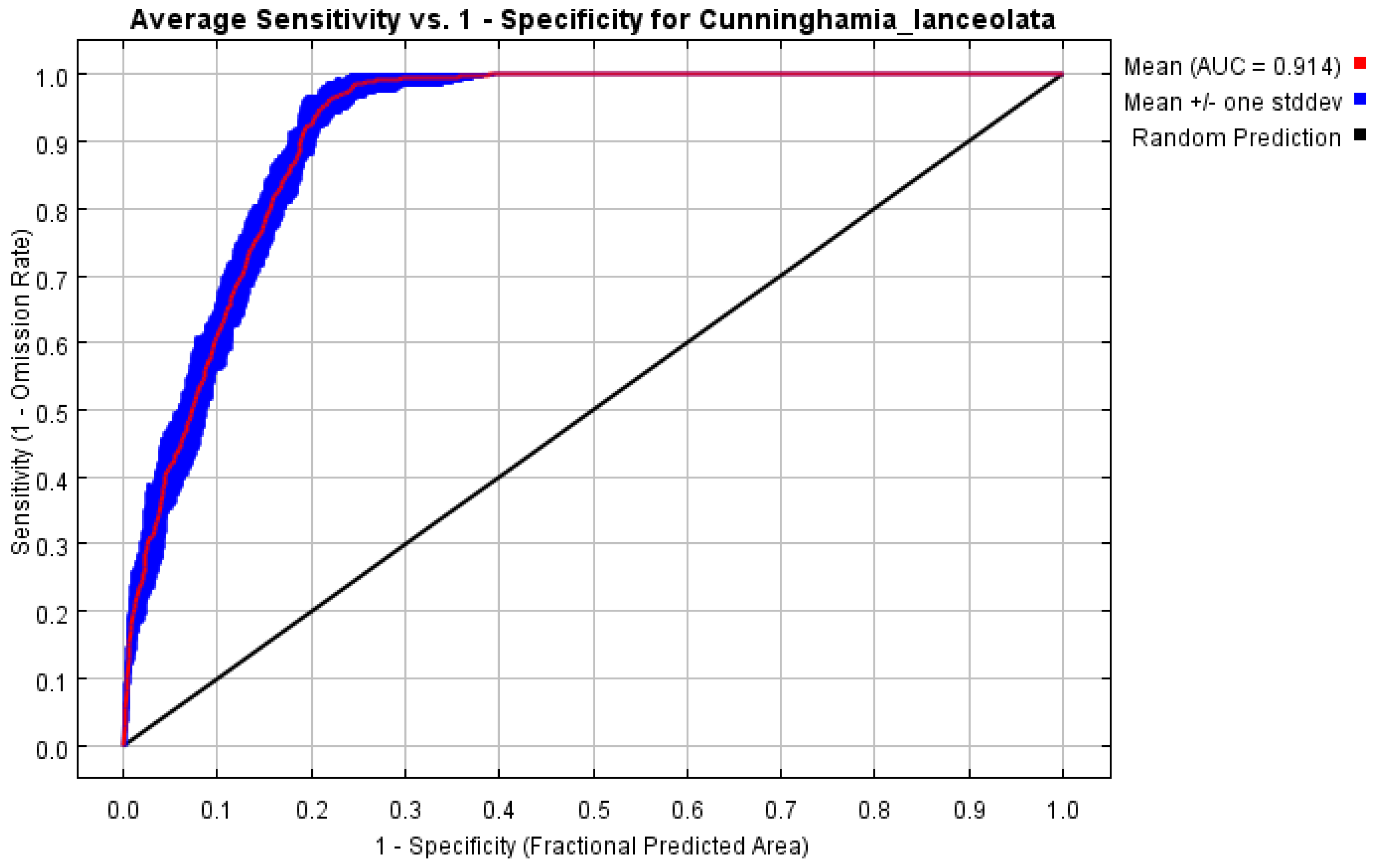
The performance of the model can be analyzed by the receiver operating characteristic curve (ROC) and the area under the ROC curve (AUC), where the AUC value ranges from 0 to 1. The performance of the model was classified as follows: failing (0.5–0.6), poor (0.6–0.7), fair (0.7–0.8), good (0.8–0.9), and excellent (0.9–1.0), with AUC values closer to 1, indicating more accurate prediction results.
The output in raster format was loaded into ArcGIS 10.5, which reclassified the distribution map into four classes of potential suitable zones.
2.7. Identification of Planting Area with LU Data
The LU data (2015) were loaded into ArcGis under four categories: 1. farmland; 2. bare land; 3. woodland; 4. grassland. As is the policy in China, farmland will be conserved; thus, these areas will not be available for the planting of C. lanceolata in the future. Consequently, the bare land, woodland, and grassland were assumed to have potential for the future planting of C. lanceolata. Calculations of the area of bare land, woodland, and grassland were based on the prediction of BCC-CSM2-MR, CanESM5, and MRI-ESM2-0 under SSP1-2.6, SSP2-4.5, SSP3-7.0, and SSP5-8.5 socio-shared pathways, respectively.
3. Results
3.1. Model Evaluations and Critical Environmental Variables
The Maximum Entropy model was employed to predict potential habitats with a mean AUC of 0.914 (Figure 2). The mean AUC values for the MaxEnt models of C. lanceolata were significantly higher than the random prediction value (0.5). The prediction results were very accurate, which also meant that the results of the potential distribution area made by MaxEnt were reliable.
MaxEnt corrects the adjustment of individual evaluation factors and coefficients in the model prediction using an iterative algorithm and calculates the contribution of environmental factors to the prediction.
The Table 1. showed that the precipitation of the driest month (bio14, 58%), minimum temperature of the coldest month (bio6, 24.4%), and mean diurnal range (bio2, 4.7%) were the top three environmental data used in the prediction of the MaxEnt model that affected the distribution of C. lanceolata, with a cumulative contribution of 87.1%.
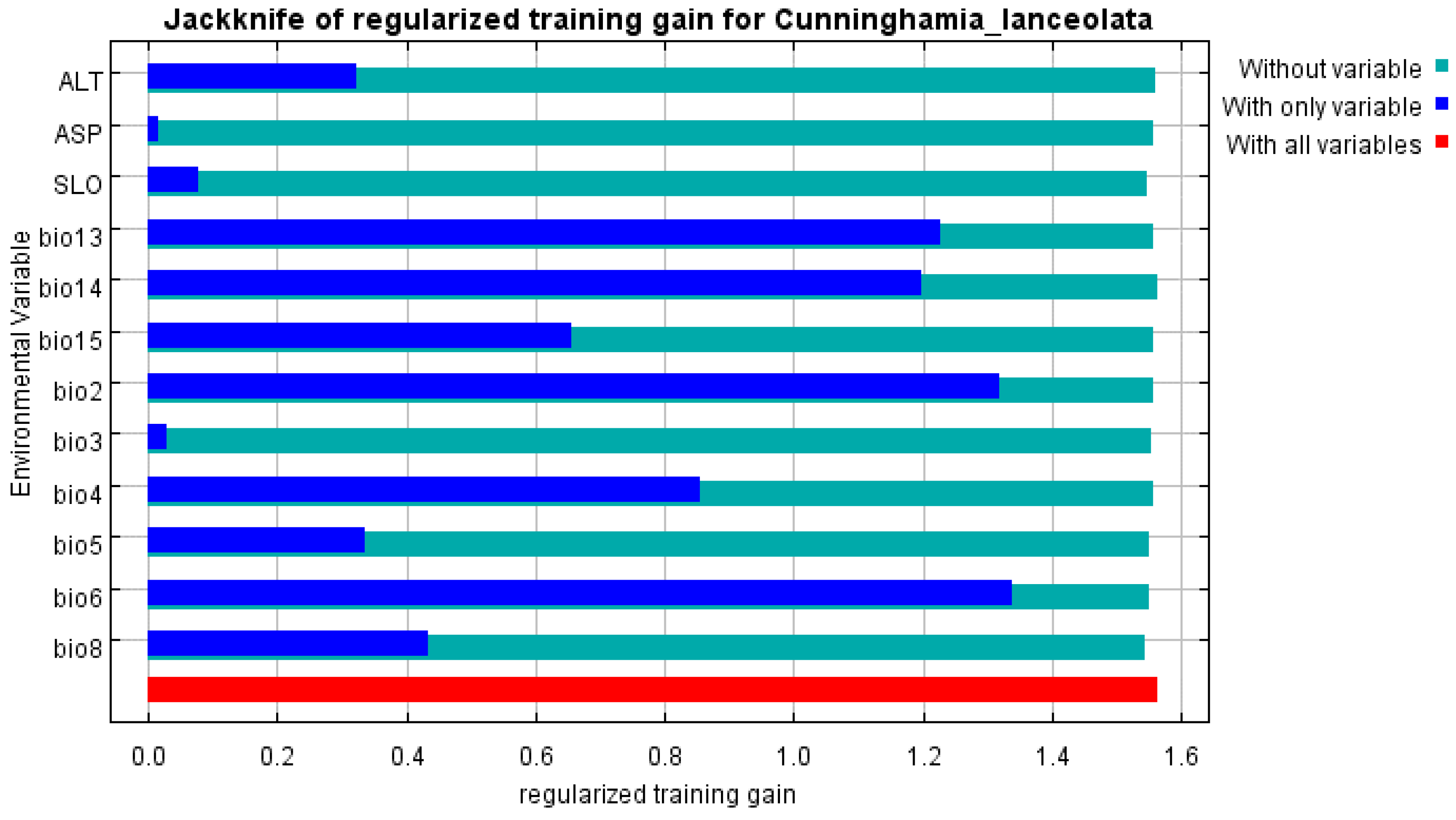
The jackknife results (Figure 3) showed that the dominant environmental variables, which influenced the habitat of C. lanceolata, were the minimum temperature of the coldest month (bio6), mean diurnal range (bio2), precipitation of the wettest month (bio13), precipitation of the driest month (bio14), and temperature seasonality (bio4). In summary, temperature, precipitation, and temperature differences were the main factors that limited the selection of suitable areas for C. lanceolata.
According to the response curves for environmental variables in MaxEnt, the probabilities for the presence of C. lanceolata in China could be assessed. When the presence probability of C. lanceolata was greater than 0.1, the corresponding environmental variable value was the critical value for C. lanceolata. The mean diurnal range (mean of monthly (max temp-min temp)) (bio2) appropriate for the growth of C. lanceolata was found to range from 3.3 °C to 10.6 °C. When the mean diurnal range (mean of monthly (max temp-min temp)) (bio2) was 5.77, the probability of the presence of C. lanceolata attained the maximum value. The seasonal temperature (standard deviation * 100) (bio4) that was suitable for the growth of C. lanceolata ranged from 1.4 to 9.5 °C. The maximum temperature of the warmest month (bio5) appropriate for the growth of C. lanceolata was found to range from 17.4 °C to 35.5 °C. The minimum temperature of the coldest month (bio6) > −5.4 °C was suitable for the growth of C. lanceolata. The threshold value of precipitation of wettest month (bio13) appropriate for the growth of C. lanceolata was 157.8 mm, whereas the threshold value of the precipitation of the driest month suitable for the growth of C. lanceolata was 5.5 mm (Figure 4).
3.2. Current Potential Distribution
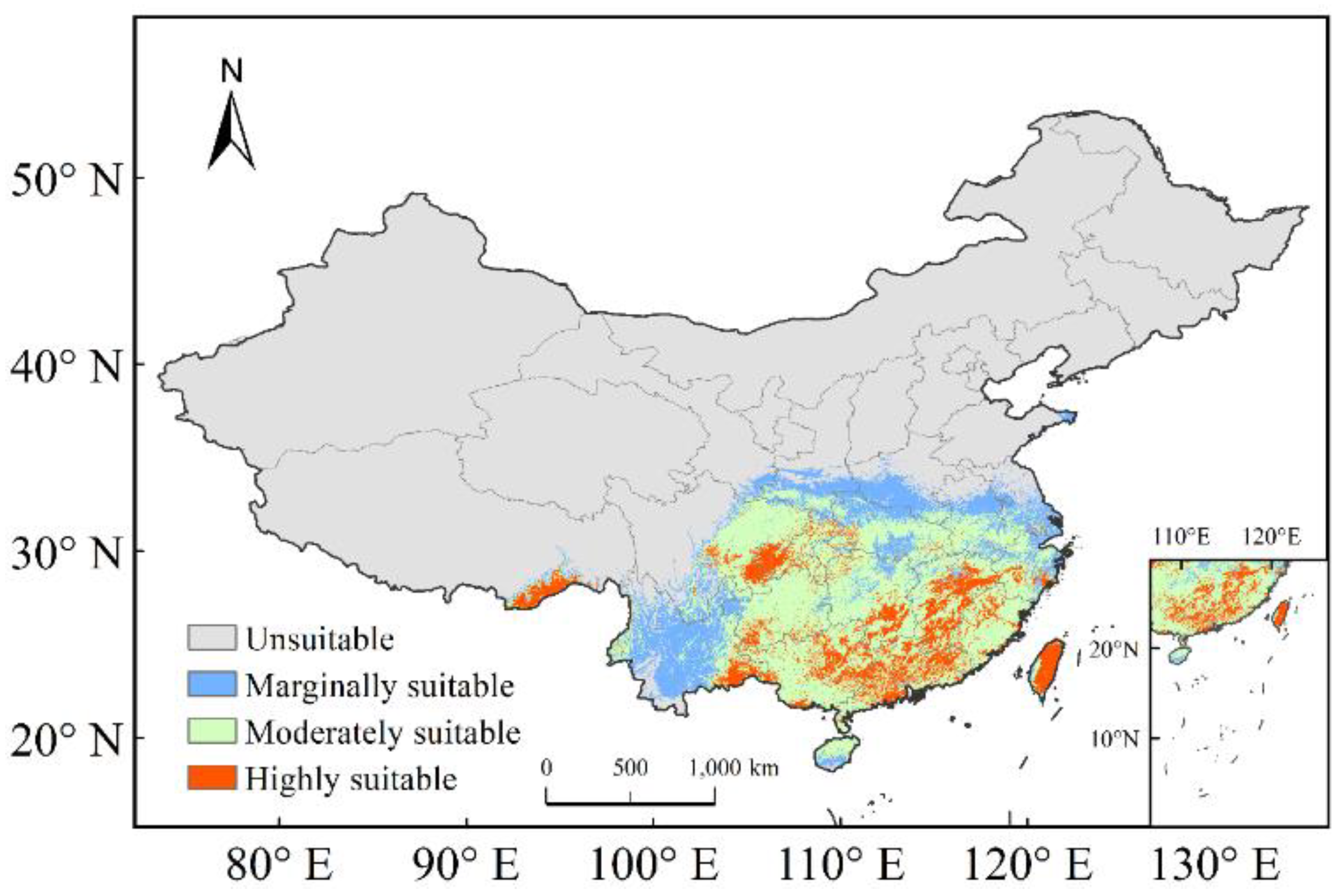
The current potential distribution map for C. lanceolata in China is shown in Figure 5, where unsuitable, marginally suitable, moderately suitable, and highly suitable areas comprised 743.30 × 10⁴ km2, 57.89 × 10⁴ km2, 120.63 × 10⁴ km2, 39.57 × 10⁴ km2, which accounted for 77%, 6%, 13%, 4% of the total suitable area in China, respectively.
The highly suitable areas for C. lanceolata in China were found to be primarily located in Southeastern Tibet; Central and Western Chongqing; Southeastern Yunnan; Southeastern Sichuan; southwestern Guizhou; Southern and Central Hunan; Southern, Northeastern Guangxi; Central and Northern Guangdong; Central Hong Kong; Central, Southern and Eastern Jiangxi; Central Fujian; as well as Central Zhejiang and Taiwan Provinces.
Moderately suitable areas for C. lanceolata in China were found to be mainly located in Western and Eastern Yunnan; Eastern and Southern Sichuan; Southern Shanxi; Chongqing; Central and Eastern Hubei; Western, Central and Eastern Anhui; Northeastern, Northwestern and Central Zhejiang; Central and Northern Hainan; Guizhou; Guangxi; Hunan; Guangdong; Hunan; Jiangxi; Fujian Provinces.
3.3. Potential Future Distribution Areas
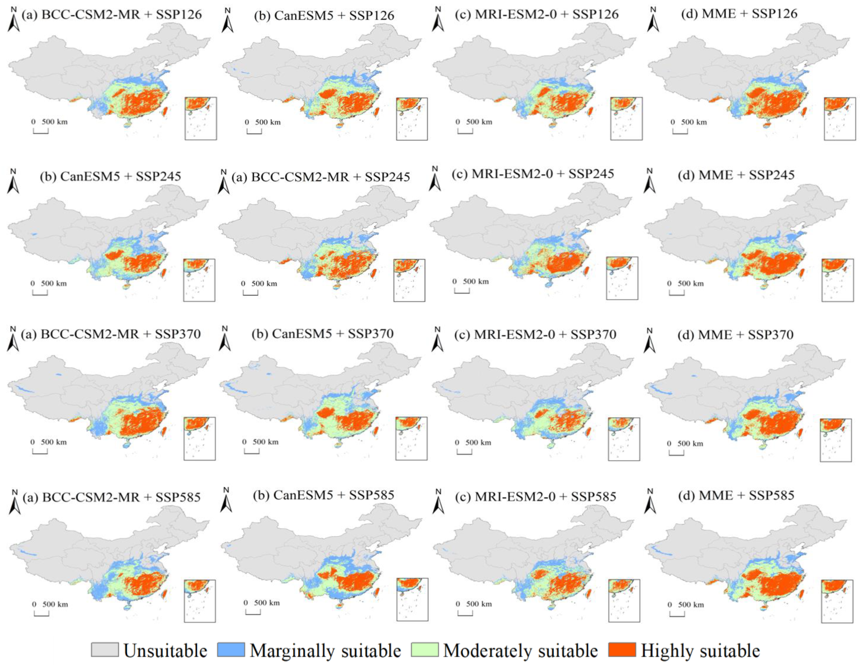
The predictions of suitable areas for C. lanceolata in 2041–2060 according to BCC-CSM2-MR (Beijing Climate Center, China), CanESM5 (Canadian Centre for Climate Modelling and Analysis, Canada), and MRI-ESM2-0 (Meteorological Research Institute, Japan) climate data under SSP1-2.6, SSP2-4.5, SSP3-7.0, and SSP5-8.5 are shown in Figure 6.
An analysis of the prediction of BCC-CSM2-MR under different SSPs revealed that the maximum threshold of suitable areas was attained under SSP3-7.0, with the minimum under SSP5-8.5. Compared to the prediction of SSP1-2.6, the highly suitable and moderately suitable areas increased slightly under SSP2-4.5 and SSP3-7.0. Under SSP2-4.5, the highly suitable and moderately suitable areas obtained the maximum value between four SSPs, after which they both decreased dramatically to 100.45 × 10⁴ km2 and 57.10 × 10⁴ km2, respectively, under the SSP5-8.0. Meanwhile, the marginally suitable area under SSP3-7.0 increased to 15.11 × 10⁴ km2 and obtained the maximum value between the four SSPs. Through observations and comparisons (Figure 6), it was found that the highly suitable zones in Guangxi, Tibet, and Anhui Provinces were degraded to moderately or marginally suitable zones. Furthermore, the moderately suitable zones in the Sichuan, Guangxi, and Anhui Provinces were degraded to marginally suitable zones under the high radiative forcing scenario (SSP5-8.5). This indicated that the highly radiative forcing environment had a negative effect on C. lanceolata.
Conversely, the prediction of the CanESM5 model under different SSPs revealed that the total of suitable areas attained a maximum under SSP3-7.0, and the minimum under SSP5-8.5 was the same as the prediction of the BCC-CSM2-MR model. The highly suitable area reached the maximum value under SSP1-2.6, whereas the total of moderately suitable and suitable areas simultaneously reached the maximum under SSP3-7.0. Under SSP5-8.5, the total suitable zone was the smallest, whereas the marginally suitable zone was the largest. Finally, according to the prediction of MRI-ESM2-0, the highly suitable area and sum of the suitable area attained their maximum under SSP2-4.5, and the marginally suitable area reached the minimum under SSP3-7.0.
An assessment of the prediction results of the three models under the four SSPs found that under SSP5-8.0, the prediction of the two models showed that the marginally suitable zone obtained its maximum, and there was no indication that the highly suitable zone obtained its maximum. Meanwhile, the average values of suitable and highly suitable areas in three models under SSP5-8.0 were the smallest between the four SSPs, which signified that the high radiative forcing had a negative effect on C. lanceolata. This initiated the degradation of highly or moderately suitable zones, predominantly located in Guangxi, Shanxi, Sichuan, and Jiangsu, to marginally suitable or unsuitable zones.
The arithmetic average values of highly suitable areas of the three models under SSP1-2.6 reached their maximum and their standard deviations were quite small, which further indicated that the prediction was very convincing. This showed that the environment with a low radiative forcing and a 2 °C increase in temperature would effectively enlarge the highly suitable zone for C. lanceolata. The arithmetic average of its total suitable area predicted by the three models under SSP1-2.6 was not the largest between the four SSPs; it was 15.79 × 10⁴ km2 less than the maximum value predicted under SSP3-7.0. The precipitation, temperature, and other environmental factors in the highly suitable zone had a positive impact on the growth of C. lanceolata, which indicated that the density, growth rate, or wood quality of C. lanceolata in highly suitable zones would be better than those in other suitable zones. Therefore, the low intensity of radiative forcing environment was best for the expansion of the suitable area for C. lanceolata. However, there was no significant difference between the moderately suitable area predicted under SSP2-4.5, and SSP3-7.0.
3.4. Future Changes in Suitable Habitats
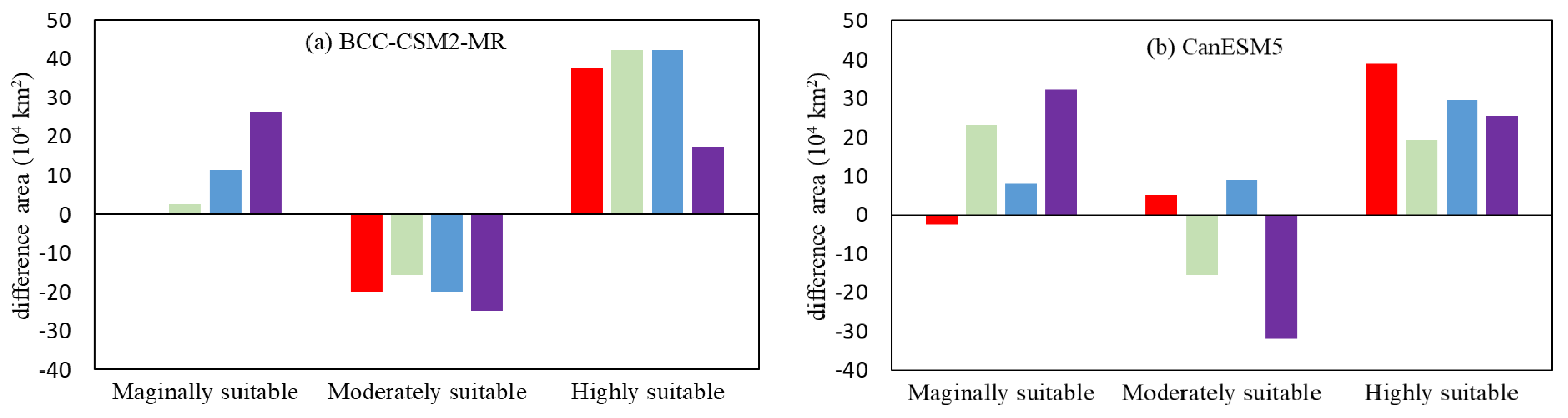
Figure 7 has shown the future changes in suitable habitats in the future. From 2041–2060, the prediction of the BCC-CSM2-MR model under the SSP1-2.6 scenario indicated that the lost suitable habitat area of C. lanceolata would be 7.71 × 10⁴ km2, whereas the gained area would be 25.60 × 10⁴ km2. The lost area was primarily located in South Yunnan, where there was a marginally suitable area for C. lanceolata. The gained area was mainly concentrated in Southwestern and Eastern Shandong, as well as West and South Henan, which became a marginally suitable area for C. lanceolata. There were 0.39 × 10⁴ km2 of marginally suitable area gained, 20.07 × 10⁴ km2 of moderately suitable area lost, and 37.69 × 10⁴ km2 of highly suitable area gained (Figure 8). The increased area of the highly suitable area was primarily located in Hunan and Guangxi Provinces.
The prediction of BCC-CSM2-MR under SSP2-4.5 showed that there were 3.14 × 10⁴ km2 of suitable area lost and 32.26 × 10⁴ km2 gained. The lost area was mainly located in Eastern Jiangsu, where there was a marginally suitable area. The gained area was primarily located in Southern Shandong, Southern Shanxi, and Southern Yunnan, which became marginally suitable areas. There were 2.59 × 10⁴ km2 of marginally suitable area gained, 15.59 × 10⁴ km2 of moderately suitable area lost, and 42.34 × 10⁴ km2 of highly suitable area gained. The increased area of the highly suitable area was mainly located in Southern Anhui, as well as South and Central Guizhou, Fujian, Zhejiang, Hunan, and Guangxi Provinces.
The prediction of BCC-CSM2-MR under SSP3-7.0 revealed that there were 2.12 × 10⁴ km2 of suitable area lost, and 35.56 × 10⁴ km2 gained. In contrast to the other models, some of the gained area was located in Xinjiang Province. There were 11.37 × 10⁴ km2 of marginally suitable area gained, 20 × 104 km2 of moderately suitable area lost, and 42.30 × 10⁴ km2 of highly suitable area gained. The marginally suitable area was located in Hubei, Southern Shanxi, whereas Southern Henan changed to a moderately suitable area, which caused a decrease in the marginally suitable area and increase in the moderately suitable area.
The prediction of BCC-CSM2-MR under SSP5-8.5 showed that there were 5.56 × 10⁴ km2 of suitable area lost and 24.72 × 10⁴ km2 gained. The lost area was mainly located in Southern Jiangsu and the gained area was mostly located in Southern Shandong, Southern Shanxi, and Southern Yunnan. There was a 26.48 × 10⁴ km2 increase of marginally suitable area, 24.75 × 10⁴ km2 decrease in moderately suitable area, and 17.61 × 10⁴ km2 increase of highly suitable area.
The following conclusions were drawn by analyzing the data: 1. The suitable distribution areas increased in the prediction of BCC-CSM2-MR model under four future sharing-economic scenarios, which were mainly located in Southern Gansu, Shanxi, Eastern Shandong, as well as Western and Southern Henan. Under the SSP3-7.0, the increased area attained a maximum of 33.44 × 10⁴ km2. 2. The moderately suitable area decreased in all four SSP scenarios. Meanwhile, the highly suitable and marginally suitable areas increased. The growth value of the highly suitable area was far greater than that of the marginally suitable area, except under the SSP5-8.0 scenario.
The prediction of the CanESM5 model under SSP1-2.6 showed that there were 0.72 × 10⁴ km2 of suitable area lost and 41.95 × 10⁴ km2 gained. Except for this gained area, Southern Hebei became the marginally suitable area for C. lanceolata. The marginally suitable area decreased by 2.49 × 10⁴ km2, whereas the moderately suitable area increased by 5.05 × 10⁴ km2, and the highly suitable area increased by 38.93 × 10⁴ km2. The newly increased highly suitable area was primarily located in the Eastern and Central Sichuan Province.
The prediction of the CanESM5 model under SSP2-4.5 revealed that there were 6.05 × 10⁴ km2 of suitable area lost and 32.92 × 10⁴ km2 gained. There was a 23.04 × 10⁴ km2 increase in marginally suitable area, a 15.40 × 10⁴ km2 decrease in moderately suitable area, and a 19.40 × 10⁴ km2 increase in highly suitable area.
The prediction of the CanESM5 model under SSP3-7.0 indicated a 6.34 × 10⁴ km2 loss in a suitable area, and 52.84 × 10⁴ km2 gained in suitable area compared with now. The marginally suitable area increased by ~8.13 × 10⁴ km2, moderately suitable area increased by 8.97 × 10⁴ km2, and the highly suitable area increased by 29.67 × 10⁴ km2. Compared with the predictions under SSP1-2.6 and SSP2-4.5, the marginally suitable area along the coast was upgraded to moderately suitable.
The prediction of the CanESM5 model under SSP5-8.5 showed that there were 7.06 × 10⁴ km2 in suitable area lost and 32.63 × 10⁴ km2 gained compared with now. There was an increase of 32.32 × 10⁴ km2 in marginally suitable area, a 32.00 × 10⁴ km2 decrease in moderately suitable area, and an increase of 25.42 × 10⁴ km2 in the highly suitable area.
An analysis of the prediction results of the CanESM5 under the four SSPs led to the following conclusions: 1. The suitable area increased in the future, which was similar to the prediction of BCC-CSM2-MR. 2. Unlike the prediction of BCC-CSM2-MR, the lost area predicted by the CanESM5 was principally located in Central Hubei, Northern Hunan, Southern Jiangsu, Central Anhui, and Southern Henan.
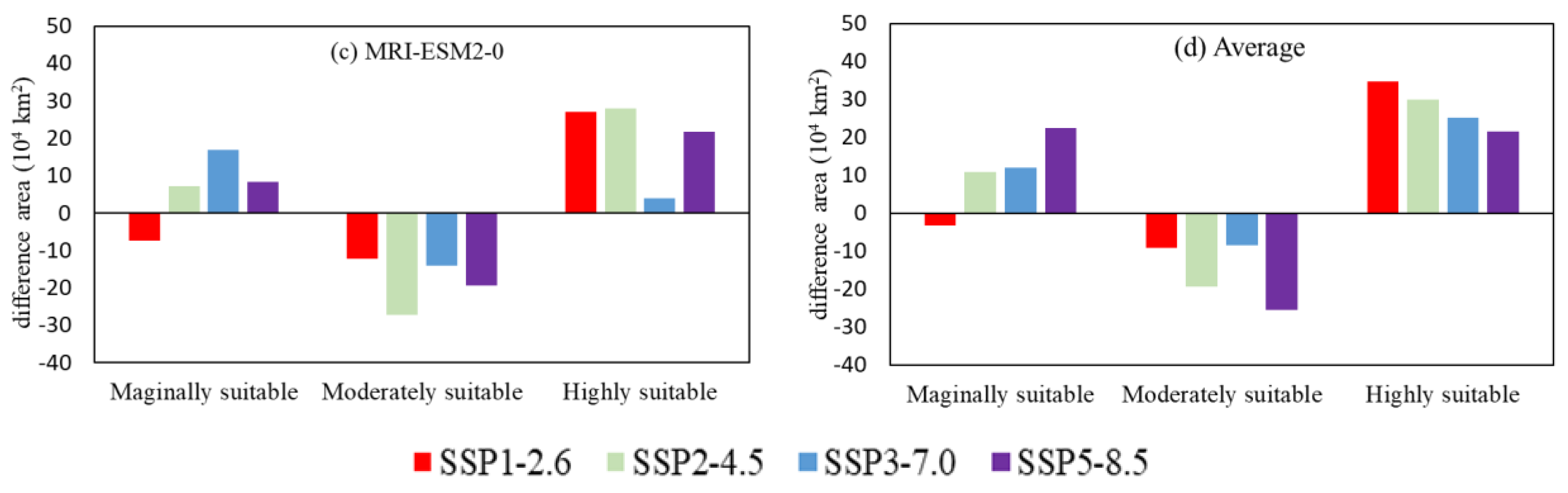
The predictions of the MRI-ESM2-0 model under SSP1-2.6 showed a suitable area loss of 4.10 × 10⁴ km2 and 11.33 × 10⁴ km2 gained compared with now. There was a decrease of 7.30 × 10⁴ km2 in marginally suitable area, a 12.36 × 10⁴ km2 increase in moderately suitable area, and a 27.11 × 10⁴ km2 increase in highly suitable area.
The prediction of the MRI-ESM2-0 model under the SSP2-4.5 showed that there were 14.24 × 10⁴ km2 of suitable area lost and 21.84 × 10⁴ km2 gained compared with now. There was an increase of 7.06 × 10⁴ km2 in marginally suitable area, a 27.24 × 10⁴ km2 decrease in the moderately suitable area, and an increase of 27.86 × 10⁴ km2 in highly suitable area.
The prediction of the MRI-ESM2-0 model under the SSP3-7.0 revealed that there were 12.02 × 10⁴ km2 of suitable area lost and 18.46 × 10⁴ km2 gained compared with now. There was an increase of 16.80 × 10⁴ km2 in marginally suitable area, a decrease of 14.05 × 10⁴ km2 in a moderately suitable area, and an increase of 3.81 × 10⁴ km2 in a highly suitable area.
The prediction of the MRI-ESM2-0 model under the SSP5-8.5 showed that there were 6.78 × 10⁴ km2 in suitable area lost and 17.27 × 10⁴ km2 gained compared with now. There was an increase of 8.39 × 10⁴ km2 in a marginally suitable area, a decrease of 19.48 × 10⁴ km2 in a moderately suitable area, and an increase of 21.76 × 10⁴ km2 in highly suitable area.
3.5. Practical Available Planting in the Predicted Suitable Area
The Table 2 shows the predicted average areas combined with land use types. Under SSP1-2.6, the average areas of farmland, woodland, grassland, and bare land for the three models were 78.52 × 10⁴ km2, 119.39 × 10⁴ km2, 26.93 × 10⁴ km2, and 0.04 × 10⁴ km2, respectively. Among the three models, the results of the CanESM5 model were generally higher. For example, the projected woodland, grassland, and bare land area were 125.57 × 10⁴ km2, 30.81 × 10⁴ km2, and 0.05 × 10 4 km2, respectively. The practical available area under SSP1-2.6 for the planting of C. lanceolata was 146.36 × 10⁴ km2, which was 60.25% of the theoretical value.
The prediction under SSP2-4.5 revealed that the average areas of farmland, woodland, grassland, and bare land in the three models were 74.78 × 10⁴ km2, 122.50 × 10⁴ km2, 28.88 × 10⁴ km2, and 0.04 × 10⁴ km2, respectively. Approximately 62.59% of the theoretical area (151.42 × 10⁴ km2) would be practically available for the planting of C. lanceolata under SSP2-4.5.
Under the condition of SSP3-7.0, the projected farmland, woodland, grassland, and bare land were 77.49 × 10⁴ km2, 123.20× 10⁴ km2, 29.95 × 10⁴ km2, and 0.1 × 10⁴ km2, on average. The practical available area under SSP3-7.0 for the planting of C. lanceolata was 153.25 × 10⁴ km2, which was 61.41% of the theoretical value. The prediction from CanESM5 performed better between the three models under SSP3-7.0, which had 162.45 × 10⁴ km2 available for the planting of C. lanceolata.
The prediction under SSP5-8.5 indicated an average farmland area in the three models of 72.87 × 10⁴ km2, an average woodland area of 121.98 × 10⁴ km2, average grassland area of 28.16 × 10⁴ km2, and average bare land area of 0.05 × 10⁴ km2. The practical available area under SSP5-8.5 for the planting of C. lanceolata was 150.19 × 10⁴ km2, which was 62.80% of the theoretical value.
4. Discussion
Global climate change is caused by both natural dynamics and anthropogenic activities. The increase of carbon dioxide and other greenhouse gases has been evident on a global scale. The Chinese government has issued a series of policies to reduce greenhouse gas emissions and revert grain plots to forestry.
In recent years, plantation areas have increased, as afforestation has proven to be one of the most effective and ecologically compatible practices for the enhancement of carbon sequestration in terrestrial ecosystems. C. lanceolata is an excellent fast-growing conifer species that is unique to Southern China and is naturally distributed in the region between 101°13′ and 121°53′ E and 19°30′ and 34°03′ N, which has a long history in China [50]. Furthermore, C. lanceolata is not only important for timber production, but also for soil and water conservation, and land restoration. In addition to ecological functions, C. lanceolata is an ideal choice for roadside trees and the establishment of windbreaks, due to its strong adaptability, including robust wind and smoke resistance. The growth process of the C. lanceolata forest mainly includes seedling stage, quick-growing stage, mature stage and senescence stage. In 2–3 years after planting, C. lanceolata forest at the seedling stage and the quick-growing stage of C. lanceolata is from 3–4 years to 10–15 years after planting. In this stage, the height and diameter of C. lanceolata increase rapidly. From 10–15 to 25–30 years, the volume of C. lanceolata reached its maximum. C. lanceolata forests usually become mature after 30–40 years, and the growth of volume decreases slowly. After 60 years, the growth of C. lanceolata forests decreases sharply and enters the senescence stage.
It is critical to have a clear understanding of the suitable growth areas for C. lanceolata and to protect existing stands, while simultaneously increasing planted areas and economic income. However, there has been limited research focused on predicting suitable growth areas for C. lanceolata in China. Li et al. [31] employed the representative concentration pathways (RCPs) from the Beijing Climate Center Climate System model version 1.1 (BCC-CSM1-1) data to predict suitable distribution areas of C. lanceolata in China for three time periods (present day, 2041–2060, and 2061–2080). The MaxEnt parameters were optimized, and the prediction indicated that the suitable growth area for C. lanceolata exhibited a trend to move northward and became more fragmentated over time. However, the prediction based on the single global climate model was inevitably uncertain under certain extreme conditions. Furthermore, due to the lack of suitable data, the effects of anthropogenic activities on the species distribution were not considered in the research.
For this study, multiple global climate models and the latest CMIP6 data were used to predict the suitable growth areas of C. lanceolata. Furthermore, the LU data were combined with the prediction results to evaluate the effects of human activities on species distribution.
The most important bioclimatic variables affecting the presence of C. lanceolata were the precipitation of the driest month (bio14), and the minimum temperature of the coldest month (bio6). These results were similar to those of previous research [56,57]. The precipitation of the driest month at lower than 5.51 mm greatly decreased the probability of the presence of C. lanceolata.
Temperature is one of the most critical environmental factors that impacts the photosynthetic physiology and ecology of plants. Plants must reside within a certain temperature range to perform photosynthesis, and each possesses a lowest, most suitable, and highest temperature threshold [58]. A minimum temperature of the coldest month (bio6) higher than −5.4 °C greatly increases the probability of the presence of C. lanceolata. Temperature affects the photosynthetic mechanism, because many components of photosynthetic metabolism are highly temperature sensitive [59]. Low temperature can reduce the hydrolysis and transport of starch accumulated within the chloroplast, then decrease the rate of photosynthetic [60]. On the contrary, the rate of photosynthetic increases responses to the increase of temperature until reaching a thermal optimum, after which rates decline due to enzyme deactivation at increasingly high temperatures. Enzyme degradation at high temperatures can decrease electron transport rates and decrease chlorophyll content [61].
By analyzing the predictions of different models under the same scenario, it is found that prediction results are various. For example, in SSP1-2.6 scenario, the predicted results of the BCC-CSM2-MR and MRI-ESM2-0 model showed that the area of moderately suitable area of C. lanceolata will decrease in the future, but the predicted results of the CanESM5 model showed that it will increase slightly in the future. Conversely, in the SSP5-8.5 scenario, the prediction results of the three models are consistent in the change of the marginally suitable area, moderately suitable area and highly suitable area (increase or decrease at the same time). It is hard to find a regular trend or result based on the prediction of any single model.
However, after averaging the prediction results of the three models, a unified trend can be found. It also proves that the prediction of multi-model can avoid the single model’s uncertainty and show a trend that are more likely to happen in the future. In the SSP scenario with higher radiative forcing, the increase area of marginally suitable area is larger, while under the SSP scenario with lower radiative forcing, the increased area of highly suitable area is larger. The prediction of SSP5-8.5 lost the largest moderately suitable area and the SSP3-7.0 lost the smallest moderately suitable area. The reason caused the trend between different SSP scenario not only to be radiative forcing, but also the societies with different development pathways in the future. SSP1 represents a society that makes a shift to sustainable development. Conversely, the SSP2 depicts a society that develops following a historical pattern without substantial future deviations. SSP3 and 4 represent societies with rapidly growing populations and low investments in health or education. SSP5 assumes a social economy that is based on fossil fuels and intensive energy use. The more environmentally friendly a society is, the more increased a highly suitable area of C. lanceolata will be. On the contrary, the highly suitable area and moderately suitable area would degenerate, resulting in the increase of a marginally suitable area.
Although the predicted results of four scenarios showed that the suitable area of C. lanceolata will increase from 2041–2060, considering the longevity and life-cycle of C. lanceolata, the predicted results may have a lag period, because the C. lanceolata generally enters the stage of flowering and fruiting after 6–10 years of planting, and remains stable during 15–40 years after planting. However, most C. lanceolata are planted artificially in China, not naturally propagated. A variety of artificial cultivation techniques of C. lanceolata are mature and universal in China. This can greatly shorten the lag period of prediction.
5. Conclusions
For this study, the potential future suitable growth area of C. lanceolata was predicted using a MaxEnt model based on three GCM models under different scenarios from 2041–2060 in China. The major conclusions were summarized as follows:
- (1)
- The current potential suitable growth areas for C. lanceolata were mainly located in Southern China. The annual temperature range was the most important variable to affect the potential suitable area of C. lanceolata. The current potential highly suitable area of C. lanceolata was primarily located in areas with a low annual temperature range, which was in accordance with the existing distribution of C. lanceolata. When the annual temperature varied from 4.7–6.7 °C, the logistic output of MaxEnt was higher than 0.5, which indicated that the area was highly suitable for C. lanceolata. When the annual temperature varied from 3.30–10.60 °C, the logistic output of MaxEnt was higher than 0.1, which indicated that the area was suitable for C. lanceolata.
- (2)
- The suitable area of C. lanceolata was observed to increase in China under all SSPs scenarios from 2041–2060. The gained area was mainly located in Southwest and Eastern Shandong, Western and Southern Henan, Northern Anhui, Northern and Central Jiangsu, Southern Shanxi, and Southern Yunnan in most models under four SSPs, as the uncertainties were unavoidable for the prediction. However, the average of multiple models may effectively reduce the uncertainty and balance the prediction results. The average of multiple models revealed that the suitable area of C. lanceolata increased to 29.00 × 10⁴ km2 under SSP3-7.0, which was the largest between the four scenarios, whereas the increased area under SSP5-8.5 was the smallest between the four scenarios at 18.59 × 10⁴ km2. This result revealed that the extremely high radiative forcing had a serious negative effect on C. lanceolata. Conversely, under SSP1-2.6, which had a low radiation intensity and effective control of global temperature growth at 2 °C, the growth area of the highly suitable area was the largest, increasing by 34.61 × 10⁴ km2. The highly suitable area possessed various environmental factors that were more suitable for the growth of C. lanceolata, which cultivated higher quality trees, a faster growth rate, and higher timber yields. Consequently, the increased highly suitable area of C. lanceolata under SSP1-2.6 had important economic and ecological value, which could not be ignored. As described above, the suitable area and yield of C. lanceolata were greatly increased under the SSP1-2.6 and SSP3-7.0 in different ways.
- (3)
- The LUCC data were reclassified into four categories: farmland, bare land, forest land, and grassland. In view of China’s arable land protection red line policy, the bare land, woodland, and grassland might be potentially available for the planting of C. lanceolata in the future. When the predictions were combined with the reclassified land use data, the result showed that the average practical available area for C. lanceolata would be approximately 61.76% of the predicted suitable area. However, with the further promotion of the policy of returning farmland to forests in China, progressively more grain plots would be returned to forestry and public awareness of forest protection would be enhanced. The practical available planting area and distribution of C. lanceolata in China will increase significantly in the future.
Author Contributions
Conceptualization, Z.Z. and Y.Z.; methodology, Y.Z.; software, Y.Z. and B.Z.; validation, Z.Z.; formal analysis, M.G.; resources, Z.Z.; data curation, Y.Z. and X.C.; writing—original draft preparation, Y.Z.; writing—review and editing, Z.Z., Y.Z. and X.C.; visualization, B.Z.; supervision, Z.Z.; project administration, R.K., L.Y.; funding acquisition, Z.Z. All authors have read and agreed to the published version of the manuscript.
Funding
This work was supported by the National Key Research and Development Project of China (grant numbers 2019YFC0409004), National Natural Science Foundation of China (grant number 41971025) and the Priority Academic Program Development of Jiangsu Higher Education Institutions (PAPD).
Data Availability Statement
The data presented in this study are available on request from the corresponding author.
Conflicts of Interest
The authors declare no conflict of interest.
Appendix A

Table A1.
Environmental variables for habitat suitability modeling of C. lanceolata.
| Type | Variable | Description | Source | Unit |
|---|---|---|---|---|
| Bioclimatic Variables | bio01 | Annual mean temperature | WorldClim | °C |
| bio02 | Mean diurnal range (mean of monthly (max temp-min temp)) | WorldClim | °C | |
| bio03 | Isothermality (bio2/bio7) (*100) | WorldClim | - | |
| bio04 | Temperature seasonality (standard deviation*100) | WorldClim | °C | |
| bio05 | Max temperature of warmest month | WorldClim | °C | |
| bio06 | Min temperature of coldest month | WorldClim | °C | |
| bio07 | Temperature annual range (bio5–bio6) | WorldClim | °C | |
| bio08 | Mean temperature of wettest quarter | WorldClim | °C | |
| bio09 | Mean temperature of driest quarter | WorldClim | °C | |
| bio10 | Mean temperature of warmest quarter | WorldClim | °C | |
| bio11 | Mean temperature of coldest quarter | WorldClim | °C | |
| bio12 | Annual precipitation | WorldClim | mm | |
| bio13 | Precipitation of wettest month | WorldClim | mm | |
| bio14 | Precipitation of driest month | WorldClim | mm | |
| bio15 | Precipitation seasonality (coefficient of variation) | WorldClim | 1 | |
| bio16 | Precipitation of wettest quarter | WorldClim | mm | |
| bio17 | Precipitation of driest quarter | WorldClim | mm | |
| bio18 | Precipitation of warmest quarter | WorldClim | mm | |
| bio19 | Precipitation of coldest quarter | WorldClim | mm | |
| Topographic Variable | ALT | Altitude | WorldClim | m |
| SLO | Slope | Derived from ALT | % | |
| ASP | Aspect | Derived from ALT | ° |
Table A2.
Multicollinearity test using Pearson correlation coefficients of twelve important environmental variables. (** and * indicate a significance level of 0.01 and 0.05, respectively).
Table A2.
Multicollinearity test using Pearson correlation coefficients of twelve important environmental variables. (** and * indicate a significance level of 0.01 and 0.05, respectively).
| Variables | ASP | ALT | SLO | Bio2 | Bio3 | Bio4 | Bio5 | Bio6 | Bio8 | Bio13 | Bio14 | Bio15 |
|---|---|---|---|---|---|---|---|---|---|---|---|---|
| ASP | 1 | |||||||||||
| ALT | 0.184 ** | 1 | ||||||||||
| SLO | 0.201 ** | 0.498 ** | 1 | |||||||||
| bio2 | 0.082 * | 0.311 ** | −0.038 | 1 | ||||||||
| bio3 | 0.200 ** | 0.602 ** | 0.117 ** | 0.488 ** | 1 | |||||||
| bio4 | −0.149 ** | −0.474 ** | −0.194 ** | 0.223 ** | −0.687 ** | 1 | ||||||
| bio5 | −0.068 * | −0.766 ** | −0.417 ** | 0.138 ** | −0.328 ** | 0.622 ** | 1 | |||||
| bio6 | 0.071 * | −0.248 ** | −0.166 ** | −0.436 ** | 0.349 ** | −0.653 ** | 0.134 ** | 1 | ||||
| bio8 | −0.083 * | −0.610 ** | −0.353 ** | 0.038 | −0.058 | 0.282 ** | 0.748 ** | 0.352 ** | 1 | |||
| bio13 | 0.023 | 0.013 | 0.086 * | −0.458 ** | 0.283 ** | −0.559 ** | −0.106 ** | 0.677 ** | 0.063 | 1 | ||
| bio14 | −0.023 | −0.299 ** | −0.056 | −0.481 ** | −0.198 ** | −0.077 * | 0.165 ** | 0.374 ** | 0.027 | 0.437 ** | 1 | |
| bio15 | 0.055 | 0.455 ** | 0.181 ** | 0.369 ** | 0.569 ** | −0.327 ** | −0.216 ** | 0.071 * | 0.080 * | 0.209 ** | −0.619 ** | 1 |
References
- Smeraldo, S.; Bosso, L.; Salinas-Ramos, V.B.; Ancillotto, L.; Sánchez-Cordero, V.; Gazaryan, S.; Russo, D. Generalists yet different: Distributional responses to climate change may vary in opportunistic bat species sharing similar ecological traits. Mammal. Rev. 2021. [Google Scholar] [CrossRef]
- Vermeiren, P.; Reichert, P.; Schuwirth, N. Integrating uncertain prior knowledge regarding ecological preferences into multi-species distribution models: Effects of model complexity on predictive performance. Ecol. Model. 2020, 420, 1–15. [Google Scholar] [CrossRef]
- Scholze, M.; Knorr, W.; Nigel, W.A.; Prentice, I.C. A climate-change risk analysis for world ecosystems. Proc. Natl. Acad. Sci. USA 2006, 103, 13116–13120. [Google Scholar] [CrossRef] [PubMed] [Green Version]
- Chalghaf, B.; Chlif, S.; Mayala, B.; Ghawar, W.; Bettaieb, J.; Harrabi, M.; Benie, G.B.; Michael, E.; Salah, A.B. Ecological Niche Modeling for the Prediction of the Geographic Distribution of Cutaneous Leishmaniasis in Tunisia. Am. J. Trop. Med. Hyg. 2016, 94, 844–851. [Google Scholar] [CrossRef] [PubMed] [Green Version]
- Lindner, M.; Maroschek, M.; Netherer, S.; Kremer, A.; Barbati, A.; Garcia-Gonzalo, J.; Seidl, R.; Delzon, S.; Corona, P.; Kolström, M.; et al. Climate change impacts, adaptive capacity, and vulnerability of European forest ecosystems. For. Ecol. Manag. 2010, 259, 698–709. [Google Scholar] [CrossRef]
- Hamidreza, K.; Winfried, V. Potential impacts of climate and landscape fragmentation changes on plant distributions: Coupling multi-temporal satellite imagery with GIS-based cellular automata model. Ecol. Inform. 2016, 32, 145–155. [Google Scholar] [CrossRef]
- Zhang, K.; Yao, L.; Meng, J.; Tao, J. Maxent modeling for predicting the potential geographical distribution of two peony species under climate change. Sci. Total Environ. 2018, 634, 1326–1334. [Google Scholar] [CrossRef] [PubMed]
- Su, B.; Huang, J.; Mondal, S.K.; Zhai, J.; Wang, Y.; Wen, S.; Gao, M.; Lv, Y.; Jiang, S.; Jiang, T.; et al. Insight from CMIP6 SSP-RCP scenarios for future drought characteristics in China. Atmos. Res. 2021, 250. [Google Scholar] [CrossRef]
- Taylor, K.E.; Stouffer, R.J.; Meehl, G.A. An Overview of CMIP5 and the Experiment Design. Bull. Am. Meteorol. Soc. 2012, 93, 485–498. [Google Scholar] [CrossRef] [Green Version]
- Tebaldi, C.; Debeire, K.; Eyring, V.; Fischer, E.; Fyfe, J.; Friedlingstein, P.; Knutti, R.; Lowe, J.; O’Neill, B.; Sanderson, B.; et al. Climate model projections from the Scenario Model Intercomparison Project (ScenarioMIP) of CMIP6. Earth Syst. Dyn. 2021, 12, 253–293. [Google Scholar] [CrossRef]
- Raffini, F.; Bertorelle, G.; Biello, R.; D’Urso, G.; Russo, D.; Bosso, L. From Nucleotides to Satellite Imagery: Approaches to Identify and Manage the Invasive Pathogen Xylella fastidiosa and Its Insect Vectors in Europe. Sustainability 2020, 12, 4508. [Google Scholar] [CrossRef]
- Martínez-Minaya, J.; Cameletti, M.; Conesa, D.; Pennino, M.G. Species distribution modeling: A statistical review with focus in spatio-temporal issues. Stoch. Environ. Res. Risk Assess. 2018, 32, 3227–3244. [Google Scholar] [CrossRef]
- Noma, H.; Nagashima, K.; Kato, S.; Teramukai, S.; Furukawa, T.A. Meta-analysis using flexible random-effects distribution models. J. Epidemiol. 2021. [Google Scholar] [CrossRef] [PubMed]
- Xue, Y.; Guan, L.; Tanaka, K.; Li, Z.; Chen, Y.; Ren, Y. Evaluating effects of rescaling and weighting data on habitat suitability modeling. Fish. Res. 2017, 188, 84–94. [Google Scholar] [CrossRef]
- Lecocq, T.; Harpke, A.; Rasmont, P.; Schweiger, O.; Bolliger, J. Integrating intraspecific differentiation in species distribution models: Consequences on projections of current and future climatically suitable areas of species. Divers. Distrib. 2019, 25, 1088–1100. [Google Scholar] [CrossRef]
- Jiang, Z. Spatial Structured Prediction Models: Applications, Challenges, and Techniques. IEEE Access 2020, 8, 38714–38727. [Google Scholar] [CrossRef]
- Bradie, J.; Leung, B. A quantitative synthesis of the importance of variables used in MaxEnt species distribution models. J. Biogeogr. 2017, 44, 1344–1361. [Google Scholar] [CrossRef]
- Elith, J.; Phillips, S.J.; Hastie, T.; Dudík, M.; Chee, Y.E.; Yates, C.J. A statistical explanation of MaxEnt for ecologists. Divers. Distrib. 2011, 17, 43–57. [Google Scholar] [CrossRef]
- Jackson, C.R.; Robertson, M.P. Predicting the potential distribution of an endangered cryptic subterranean mammal from few occurrence records. J. Nat. Conserv. 2011, 19, 87–94. [Google Scholar] [CrossRef] [Green Version]
- Kalboussi, M.; Achour, H. Modelling the spatial distribution of snake species in northwestern Tunisia using maximum entropy (Maxent) and Geographic Information System (GIS). J. For. Res. 2017, 29, 233–245. [Google Scholar] [CrossRef]
- Mitchell, P.J.; Monk, J.; Laurenson, L.; Chisholm, R. Sensitivity of fine-scale species distribution models to locational uncertainty in occurrence data across multiple sample sizes. Methods Ecol. Evol. 2016, 8, 12–21. [Google Scholar] [CrossRef] [Green Version]
- Préau, C.; Isselin-Nondedeu, F.; Sellier, Y.; Bertrand, R.; Grandjean, F. Predicting suitable habitats of four range margin amphibians under climate and land-use changes in southwestern France. Reg. Environ. Chang. 2018, 19, 27–38. [Google Scholar] [CrossRef]
- Kaky, E.; Gilbert, F. Using species distribution models to assess the importance of Egypt’s protected areas for the conservation of medicinal plants. J. Arid Environ. 2016, 135, 140–146. [Google Scholar] [CrossRef] [Green Version]
- Hasui, É.; Silva, V.X.; Cunha, R.G.T.; Ramos, F.N.; Ribeiro, M.C.; Sacramento, M.; Coelho, M.T.P.; Pereira, D.G.S.; Ribeiro, B.R. Additions of landscape metrics improve predictions of occurrence of species distribution models. J. For. Res. 2017, 28, 963–974. [Google Scholar] [CrossRef]
- Fitzpatrick, M.C.; Gotelli, N.J.; Ellison, A.M. MaxEnt versus MaxLike: Empirical comparisons with ant species distributions. Ecosphere 2013, 4. [Google Scholar] [CrossRef]
- Fourcade, Y.; Engler, J.O.; Rodder, D.; Secondi, J. Mapping species distributions with MAXENT using a geographically biased sample of presence data: A performance assessment of methods for correcting sampling bias. PLoS ONE 2014, 9, e97122. [Google Scholar] [CrossRef] [PubMed] [Green Version]
- Hoveka, L.N.; Bezeng, B.S.; Yessoufou, K.; Boatwright, J.S.; Van der Bank, M. Effects of climate change on the future distributions of the top five freshwater invasive plants in South Africa. S. Afr. J. Bot. 2016, 102, 33–38. [Google Scholar] [CrossRef]
- Kong, F.; Tang, L.; He, H.; Yang, F.; Tao, J.; Wang, W. Assessing the impact of climate change on the distribution of Osmanthus fragrans using Maxent. Environ. Sci. Pollut. Res. 2021. [Google Scholar] [CrossRef] [PubMed]
- Zhang, L.; Jing, Z.; Li, Z.; Liu, Y.; Fang, S. Predictive Modeling of Suitable Habitats for Cinnamomum Camphora (L.) Presl Using Maxent Model under Climate Change in China. Int. J. Environ. Res. Public Health 2019, 16, 3185. [Google Scholar] [CrossRef] [Green Version]
- Zhang, K.; Sun, L.; Tao, J. Impact of Climate Change on the Distribution of Euscaphis japonica (Staphyleaceae) Trees. Forests 2020, 11, 525. [Google Scholar] [CrossRef]
- Li, Y.; Li, M.; Li, C.; Liu, Z. Optimized Maxent Model Predictions of Climate Change Impacts on the Suitable Distribution of Cunninghamia lanceolata in China. Forests 2020, 11, 302. [Google Scholar] [CrossRef] [Green Version]
- Bağçaci, S.Ç.; Yucel, I.; Duzenli, E.; Yilmaz, M.T. Intercomparison of the expected change in the temperature and the precipitation retrieved from CMIP6 and CMIP5 climate projections: A Mediterranean hot spot case, Turkey. Atmos. Res. 2021, 256. [Google Scholar] [CrossRef]
- Wu, Y.; Zhong, P.A.; Xu, B.; Zhu, F.; Fu, J. Evaluation of global climate model on performances of precipitation simulation and prediction in the Huaihe River basin. Theor. Appl. Climatol. 2017, 133, 191–204. [Google Scholar] [CrossRef]
- Feng, J.; Lee, D.-K.; Fu, C.; Tang, J.; Sato, Y.; Kato, H.; McGregor, J.L.; Mabuchi, K. Comparison of four ensemble methods combining regional climate simulations over Asia. Meteorol. Atmos. Phys. 2010, 111, 41–53. [Google Scholar] [CrossRef]
- Katiraie-Boroujerdy, P.S.; Akbari Asanjan, A.; Chavoshian, A.; Hsu, K.l.; Sorooshian, S. Assessment of seven CMIP5 model precipitation extremes over Iran based on a satellite-based climate data set. Int. J. Climatol. 2019, 39, 3505–3522. [Google Scholar] [CrossRef]
- Sun, Q.; Miao, C.; Duan, Q. Projected changes in temperature and precipitation in ten river basins over China in 21st century. Int. J. Climatol. 2015, 35, 1125–1141. [Google Scholar] [CrossRef]
- Her, Y.; Yoo, S.H.; Cho, J.; Hwang, S.; Jeong, J.; Seong, C. Uncertainty in hydrological analysis of climate change: Multi-parameter vs. multi-GCM ensemble predictions. Sci. Rep. 2019, 9, 4974. [Google Scholar] [CrossRef] [PubMed] [Green Version]
- Ferro, C.A.T.; Stephenson, D.B.; Sansom, P.G.; Zappa, G.; Shaffrey, L. Simple Uncertainty Frameworks for Selecting Weighting Schemes and Interpreting Multimodel Ensemble Climate Change Experiments. J. Clim. 2013, 26, 4017–4037. [Google Scholar] [CrossRef] [Green Version]
- Verburg, P.H.; van de Steeg, J.; Veldkamp, A.; Willemen, L. From land cover change to land function dynamics: A major challenge to improve land characterization. J. Environ. Manag. 2009, 90, 1327–1335. [Google Scholar] [CrossRef]
- McAlpine, C.A.; Eyre, T.J. Testing landscape metrics as indicators of habitat loss and fragmentation in continuous eucalypt forests (Queensland, Australia). Landsc. Ecol. 2002, 17, 711–728. [Google Scholar] [CrossRef]
- Gobin, A.; Campling, P.; Feyen, J. Logistic modelling to derive agricultural land use determinants: A case study from southeastern Nigeria. Agric. Ecosyst. Environ. 2002, 89, 213–228. [Google Scholar] [CrossRef]
- Soares-Filho, B.S.; Cerqueira, G.C.; Pennachin, C.L. DINAMICA—A stochastic cellular automata model designed to simulate the landscape dynamics in an Amazonian colonization frontier. Ecol. Model. 2002, 154, 217–235. [Google Scholar] [CrossRef]
- Peng, J.; Pan, Y.; Liu, Y.; Zhao, H.; Wang, Y. Linking ecological degradation risk to identify ecological security patterns in a rapidly urbanizing landscape. Habitat Int. 2018, 71, 110–124. [Google Scholar] [CrossRef]
- Foley, J.A.; DeFries, R.; Asner, G.P.; Barford, C.; Bonan, G.; Carpenter, S.R.; Chapin, F.S.; Coe, M.T.; Daily, G.C.; Gibbs, H.K.; et al. Global Consequences of Land Use. Science 2005, 309, 570–574. [Google Scholar] [CrossRef] [PubMed] [Green Version]
- Tang, X.; Fehrmann, L.; Guan, F.; Forrester, D.I.; Guisasola, R.; Pérez-Cruzado, C.; Vor, T.; Lu, Y.; Álvarez-González, J.G.; Kleinn, C. A generalized algebraic difference approach allows an improved estimation of aboveground biomass dynamics of Cunninghamia lanceolata and Castanopsis sclerophylla forests. Ann. For. Sci. 2017, 74. [Google Scholar] [CrossRef] [Green Version]
- Zhou, L.; Li, S.; Jia, Y.; Heal, K.V.; He, Z.; Wu, P.; Ma, X. Spatiotemporal distribution of canopy litter and nutrient resorption in a chronosequence of different development stages of Cunninghamia lanceolata in southeast China. Sci. Total Environ. 2021, 762, 143153. [Google Scholar] [CrossRef]
- Yi, Y.J.; Zhou, Y.; Cai, Y.P.; Yang, W.; Li, Z.W.; Zhao, X. The influence of climate change on an endangered riparian plant species: The root of riparian Homonoia. Ecol. Indic. 2018, 92, 40–50. [Google Scholar] [CrossRef]
- Fotheringham, A.S.; Oshan, T.M. Geographically weighted regression and multicollinearity: Dispelling the myth. J. Geogr. Syst. 2016, 18, 303–329. [Google Scholar] [CrossRef]
- Dormann, C.F.; Elith, J.; Bacher, S.; Buchmann, C.; Carl, G.; Carré, G.; Marquéz, J.R.G.; Gruber, B.; Lafourcade, B.; Leitão, P.J.; et al. Collinearity: A review of methods to deal with it and a simulation study evaluating their performance. Ecography 2013, 36, 27–46. [Google Scholar] [CrossRef]
- Zhou, T.; Jia, X.; Liao, H.; Peng, S.; Peng, S. Effects of elevated mean and extremely high temperatures on the physio-ecological characteristics of geographically distinctive populations of Cunninghamia lanceolata. Sci. Rep. 2016, 6, 39187. [Google Scholar] [CrossRef] [PubMed] [Green Version]
- Van Vuuren, D.P.; Stehfest, E.; Gernaat, D.E.H.J.; Doelman, J.C.; van den Berg, M.; Harmsen, M.; de Boer, H.S.; Bouwman, L.F.; Daioglou, V.; Edelenbosch, O.Y.; et al. Energy, land-use and greenhouse gas emissions trajectories under a green growth paradigm. Glob. Environ. Chang. 2017, 42, 237–250. [Google Scholar] [CrossRef] [Green Version]
- Skeie, R.B.; Myhre, G.; Hodnebrog, Ø.; Cameron-Smith, P.J.; Deushi, M.; Hegglin, M.I.; Horowitz, L.W.; Kramer, R.J.; Michou, M.; Mills, M.J.; et al. Historical total ozone radiative forcing derived from CMIP6 simulations. NPJ Clim. Atmos. Sci. 2020, 3. [Google Scholar] [CrossRef]
- Eyring, V.; Bony, S.; Meehl, G.A.; Senior, C.A.; Stevens, B.; Stouffer, R.J.; Taylor, K.E. Overview of the Coupled Model Intercomparison Project Phase 6 (CMIP6) experimental design and organization. Geosci. Model. Dev. 2016, 9, 1937–1958. [Google Scholar] [CrossRef] [Green Version]
- Riahi, K.; van Vuuren, D.P. The Shared Socioeconomic Pathways and their energy, land use, and greenhouse gas emissions implications: An overview. Glob. Environ. Chang. 2017, 42, 153–168. [Google Scholar] [CrossRef] [Green Version]
- Sultana, S.; Baumgartner, J.B.; Dominiak, B.C.; Royer, J.E.; Beaumont, L.J. Potential impacts of climate change on habitat suitability for the Queensland fruit fly. Sci. Rep. 2017, 7, 13025. [Google Scholar] [CrossRef] [PubMed]
- Liu, Y.; Yu, D.; Xun, B.; Sun, Y.; Hao, R. The potential effects of climate change on the distribution and productivity of Cunninghamia lanceolata in China. Environ. Monit. Assess. 2014, 186, 135–149. [Google Scholar] [CrossRef] [PubMed]
- Coops, N.C.; Waring, R.H.; Schroeder, T.A. Combining a generic process-based productivity model and a statistical classification method to predict the presence and absence of tree species in the Pacific Northwest, USA. Ecol. Model. 2009, 220, 1787–1796. [Google Scholar] [CrossRef]
- Chang, Q.; Xiao, X.; Doughty, R.; Wu, X.; Jiao, W.; Qin, Y. Assessing variability of optimum air temperature for photosynthesis across site-years, sites and biomes and their effects on photosynthesis estimation. Agric. For. Meteorol. 2021, 298–299. [Google Scholar] [CrossRef]
- Moore, C.E.; Meacham-Hensold, K.; Lemonnier, P.; Slattery, R.A.; Benjamin, C.; Bernacchi, C.J.; Lawson, T.; Cavanagh, A.P. The effect of increasing temperature on crop photosynthesis: From enzymes to ecosystems. J. Exp. Bot. 2021, 72, 2822–2844. [Google Scholar] [CrossRef] [PubMed]
- Ikkonen, E.N.; Shibaeva, T.G.; Titov, A.F. Influence of Daily Short-Term Temperature Drops on Respiration to Photosynthesis Ratio in Chilling-Sensitive Plants. Russ. J. Plant Physiol. 2018, 65, 78–83. [Google Scholar] [CrossRef]
- Prasad, P.V.V.; Djanaguiraman, M. High night temperature decreases leaf photosynthesis and pollen function in grain sorghum. Funct. Plant Biol. 2011, 38, 993–1003. [Google Scholar] [CrossRef] [PubMed]
Figure 1.
Distribution records of C. lanceolata in China and Taiwan province with annual temperature range.
Figure 1.
Distribution records of C. lanceolata in China and Taiwan province with annual temperature range.

Figure 2.
Reliability test of the distribution model created for C. lanceolata.

Figure 3.
Jacknife test of variable importance for C. lanceolata.

Figure 4.
Response curves for the probability of presence for C. lanceolata. The red curves show the average over 10 replicate runs; blue bands show the standard deviation (SD) calculated over 10 replicates.
Figure 4.
Response curves for the probability of presence for C. lanceolata. The red curves show the average over 10 replicate runs; blue bands show the standard deviation (SD) calculated over 10 replicates.

Figure 5.
Current potential suitable areas for C. lanceolata in China.

Figure 6.
Potential suitable area for C. lanceolata in the three models and MME under four SSPs.

Figure 7.
Changes in the potential geographical distribution of C. lanceolata in the models under the different scenarios.
Figure 7.
Changes in the potential geographical distribution of C. lanceolata in the models under the different scenarios.

Figure 8.
Differences between future and current (future−current) suitable area.


Table 1.
Permutation importance of variables for modeling.
| Code | Environmental Variables | Units | Percent Contribution |
|---|---|---|---|
| bio14 | Precipitation of driest month | mm | 58 |
| bio6 | Min temperature of coldest month | °C | 24.4 |
| bio2 | Mean diurnal range | °C | 4.7 |
| SLO | Slope | % | 2.8 |
| bio3 | Isothermality(bio2/bio7) (*100) | °C | 2.7 |
| bio4 | Temperature seasonality (standard deviation*100) | °C | 2.6 |
| bio13 | Precipitation of wettest month | mm | 1.2 |
| bio5 | Max temperature of warmest month | °C | 1.2 |
| bio8 | Mean temperature of wettest quarter | °C | 1 |
| bio15 | Precipitation seasonality | 1 | 0.5 |
| ALT | Altitude | m | 0.4 |
| ASP | Aspect | ° | 0.4 |
Table 2.
Predicted area combined with land use type (‘a’ represents BCC-CSM2-MR, ‘b’ represents CanESM5, ‘c’ represents MRI-ESM2-0).
Table 2.
Predicted area combined with land use type (‘a’ represents BCC-CSM2-MR, ‘b’ represents CanESM5, ‘c’ represents MRI-ESM2-0).
| 126a | 126b | 126c | 245a | 245b | 245c | 370a | 370b | 370c | 585a | 585b | 585c | |
|---|---|---|---|---|---|---|---|---|---|---|---|---|
| Farmland | 79.62 | 85.81 | 70.11 | 79.08 | 77.38 | 67.90 | 83.52 | 82.80 | 66.15 | 74.68 | 73.35 | 70.57 |
| Bare land | 0.04 | 0.05 | 0.04 | 0.04 | 0.05 | 0.04 | 0.11 | 0.12 | 0.06 | 0.07 | 0.05 | 0.04 |
| Woodland | 115.26 | 125.57 | 117.35 | 123.89 | 123.43 | 120.19 | 121.28 | 128.05 | 120.27 | 120.17 | 126.63 | 119.14 |
| Grassland | 25.08 | 30.81 | 24.89 | 29.58 | 29.79 | 27.26 | 28.83 | 34.28 | 26.76 | 27.67 | 30.90 | 25.91 |
Publisher’s Note: MDPI stays neutral with regard to jurisdictional claims in published maps and institutional affiliations. |
© 2021 by the authors. Licensee MDPI, Basel, Switzerland. This article is an open access article distributed under the terms and conditions of the Creative Commons Attribution (CC BY) license (https://creativecommons.org/licenses/by/4.0/).
Share and Cite
MDPI and ACS Style
Zhou, Y.; Zhang, Z.; Zhu, B.; Cheng, X.; Yang, L.; Gao, M.; Kong, R. MaxEnt Modeling Based on CMIP6 Models to Project Potential Suitable Zones for Cunninghamia lanceolata in China. Forests 2021, 12, 752. https://doi.org/10.3390/f12060752
AMA Style
Zhou Y, Zhang Z, Zhu B, Cheng X, Yang L, Gao M, Kong R. MaxEnt Modeling Based on CMIP6 Models to Project Potential Suitable Zones for Cunninghamia lanceolata in China. Forests. 2021; 12(6):752. https://doi.org/10.3390/f12060752
Chicago/Turabian StyleZhou, Yichen, Zengxin Zhang, Bin Zhu, Xuefei Cheng, Liu Yang, Mingkun Gao, and Rui Kong. 2021. "MaxEnt Modeling Based on CMIP6 Models to Project Potential Suitable Zones for Cunninghamia lanceolata in China" Forests 12, no. 6: 752. https://doi.org/10.3390/f12060752
Note that from the first issue of 2016, this journal uses article numbers instead of page numbers. See further details here.