Breather Turbulence: Exact Spectral and Stochastic Solutions of the Nonlinear Schrödinger Equation

Abstract

I address the problem of breather turbulence in ocean waves from the point of view of the exact spectral solutions of the nonlinear Schrödinger (NLS) equation using two tools of mathematical physics: (1) the inverse scattering transform (IST) for periodic/quasiperiodic boundary conditions (also referred to as finite gap theory (FGT) in the Russian literature) and (2) quasiperiodic Fourier series, both of which enhance the physical and mathematical understanding of complicated nonlinear phenomena in water waves. The basic approach I refer to is nonlinear Fourier analysis (NLFA). The formulation describes wave motion with spectral components consisting of sine waves, Stokes waves and breather packets that nonlinearly interact pair-wise with one another. This contrasts to the simpler picture of standard Fourier analysis in which one linearly superposes sine waves. Breather trains are coherent wave packets that “breath” up and down during their lifetime “cycle” as they propagate, a phenomenon related to Fermi-Pasta-Ulam (FPU) recurrence. The central wave of a breather, when the packet is at its maximum height of the FPU cycle, is often treated as a kind of rogue wave. Breather turbulence occurs when the number of breathers in a measured time series is large, typically several hundred per hour. Because of the prevalence of rogue waves in breather turbulence, I call this exceptional type of sea state a breather sea or rogue sea. Here I provide theoretical tools for a physical and dynamical understanding of the recent results of Osborne et al. (Ocean Dynamics, 2019, 69, pp. 187–219) in which dense breather turbulence was found in experimental surface wave data in Currituck Sound, North Carolina. Quasiperiodic Fourier series are important in the study of ocean waves because they provide a simpler theoretical interpretation and faster numerical implementation of the NLFA, with respect to the IST, particularly with regard to determination of the breather spectrum and their associated phases that are here treated in the so-called nonlinear random phase approximation. The actual material developed here focuses on results necessary for the analysis and interpretation of shipboard/offshore platform radar scans and for airborne lidar and synthetic aperture radar (SAR) measurements.

1. Introduction

I apply the methods of nonlinear Fourier analysis (NLFA) [1,2,3,4] to the theoretical and numerical study of ocean waves. NLFA is an approach where quasiperiodic Fourier series, rather than standard Fourier series, are applied to the study of nonlinear wave dynamics. The starting place is the study of the classical so-called nonlinear integrable equations of mathematical physics. There are an infinite number of these nonlinear integrable wave equations, many of which have physical applications to water waves. These include the Korteweg-deVries (KdV), the Kadomtsev-Petviashvili (KP) and the nonlinear Schrödinger (NLS) equations. To solve these integrable wave equations, one uses the inverse scattering transform (IST) for periodic/quasiperiodic boundary conditions [5]. The IST theory is also referred to as finite gap theory (FGT), a terminology used in Russia [6,7]. An overview of theoretical and numerical methods for applications of IST to physical oceanography is given in Reference [3]. The special coherent structure solutions of the nonlinear integrable equations include solitons, kinks, breathers, superbreathers and vortices. Thus, the full nonlinear theory of wave motion uses these solutions as nonlinear basis functions that interact nonlinearly with one another, while standard Fourier analysis uses only sine waves and is therefore unable to characterize the coherent nature of water waves.

Recent papers [1,8] analyze surface wave data obtained in Currituck Sound, South Carolina and both soliton turbulence and breather turbulence were found. The data analysis methods were those of the periodic IST (also FGT) [3], which allows for nonlinear spectral decomposition of the data. The importance of these works is to: (1) establish new methods to determine the nonlinear effects at work in measured ocean wave trains and (2) to apply the methods to determine what nonlinear Fourier modes are active in a particular data set. The nonlinear Fourier modes of the NLS equation consist of (1) sine waves, (2) Stokes waves, (3) solitons, (4) breathers, and also (5) superbreathers. This contrasts to traditional Fourier analysis which projects measured data only onto simple sine waves. We now have at our disposal the mathematical methods to project data onto the nonlinear modes and this is therefore an important period in the understanding of the presence of coherent structures in ocean waves. The goal of this paper is to provide closure on a complete theoretical and numerical approach for the U. S. Navy that can be used in real time to assess the actual nonlinear spectrum of measured wind waves by shipboard radar and lidar and by synthetic aperture radar onboard airplanes.

It is important to understand what we mean by the phrase “dense breather turbulence.” This terminology suggests that the breathers in a sea state are crowded together, perhaps even overlapping each other. Such a sea state must per forza have a large number of rogue waves, the latter defined to be the central wave in a breather packet at its maximum height during the Fermi-Pasta-Ulam (FPU) cycle time: We call a sea state with dense breathers a “rogue sea.” This concept was born in our analysis of surface wave data taken in Currituck Sound [1] where about 95% of the FGT spectral components were breather trains. Basically the time series analyzed in this data set were about T = 1680 s long with a typical number of breathers $N_{\mathrm{number}\hspace{0.17em}\mathrm{FGT} \mathrm{breathers}}~200$ (this is the number of “eigenvalue pairs connected by a spine” in the FGT spectrum). The peak period ($T_p=1/f_p$, where $f_p$ is the peak spectral frequency) of the waves is about $T_p=2.5$ s, so this would suggest that there are about 3.36 waves over each 8.4 s breather interval (found from 1680 s/200 breathers). We also determine the FGT spectral properties of breather packets, one of which is the number of waves in a breather packet, that we call here $N_{\mathrm{FGT} \mathrm{num}. \mathrm{of} \mathrm{waves}/\mathrm{breather} \mathrm{packet}}~5.1$, thus suggesting considerable overlapping of the breathers in the data because 5.1 waves > 3.36 waves. This means that the breather packets are “dense” in the sense that their tails overlap the adjacent breathers. While our definition of “dense” is somewhat ad hoc, it does suffice to give the following expression for the density of breathers in the Currituck Sound data [1]:

$$D=\frac{N_{\mathrm{FGT} \mathrm{num}. \mathrm{waves}/\mathrm{breather} \mathrm{packet}}}{\frac{T}{T_p{N}_{\mathrm{number}\hspace{0.17em}\mathrm{FGT} \mathrm{breathers}}}}=\frac{5.1 \frac{\mathrm{FGT}\hspace{0.17em}\mathrm{waves}}{\mathrm{breather}\hspace{0.17em}\mathrm{packet}}}{\frac{1680 \sec }{2.5 \sec \hspace{0.17em}\cdot 200 \mathrm{breather}\hspace{0.17em}\mathrm{intervals}\hspace{0.17em}}}=\frac{5.1 \frac{\mathrm{FGT}\hspace{0.17em}\mathrm{waves}}{\mathrm{breather}\hspace{0.17em}\mathrm{packet}}}{3.36 \frac{\mathrm{FGT}\hspace{0.17em}\mathrm{waves}}{\mathrm{breather}\hspace{0.17em}\mathrm{intervals}}}=1.52 \frac{\mathrm{breather}\hspace{0.17em}\mathrm{intervals}}{\mathrm{packet}}$$

The fact that $D>1$ for the Currituck Sound data means that the breather packets are squeezed together, with overlapping tails. One presumes that there are considerable nonlinear interactions among the crowded breather trains in the time series. In the case that D << 1, we have breathers that are few in number and sparsely scattered over the length of the time series. For the case with $D=1$, the breathers are, on average, fairly evenly scattered over the time series but there is no average overlapping: This is still likely a highly nonlinear case because each breather has its own group velocity, so that some breathers will interact by catching up with slower breathers, while others will fall behind faster moving breathers, resulting in interactions. It is tempting to call the case D > 1, a rogue sea, but we have yet to carry out sufficient numerical simulations to fully understand the effect of this parameter on the intensity of the sea state and on the statistical distribution of wave amplitudes and wave heights.

The theoretical formulation given herein provides a full characterization of the nonlinear Fourier analysis (NLFA) spectrum (here the inverse scattering transform or finite gap theory spectrum with periodic/quasiperiodic boundary conditions) based on the exact nonlinear spectral solution of the NLS equation. Future efforts will include extending this work to fully two dimensions and to higher order. The physical description of NLFA spectral solutions of NLS simultaneously consists of nonlinearly interacting sine waves, Stokes waves and breather packets, all of which are viewed as nonlinear basis functions in NLFA. Because of the coherent nature of Stokes waves and breathers, we have exact spectral solutions that have remarkably complex nonlinear dynamics that resemble classical turbulence, i.e., in which one has oscillatory waves and vortices. Furthermore, we find that because of the highly random nature of complex sea states dominated by breather packets, there is the need for a stochastic formulation of the motion (see Reference [4]). To this end, I discuss the nonlinear random phase approximation for nonlinear waves and the consequent breather turbulence and discuss how to apply it to stochastic properties of the motion and to the data analysis of measured random, nonlinear ocean waves.

However, many other issues need to be addressed, some of which are discussed herein. Why are breather trains important? Because the largest breathers generate the largest waves, many of which are much larger than predicted by the Gaussian or Rayleigh distributions, commonly used for estimating large amplitudes and wave heights in ocean waves. Other important features of the method relate to the space/time dynamics of breathers (and their associated rogue waves) and the stochastic behavior of breather turbulence. This work is important because sea states of this type are “rogue seas”, i.e., those sea states that have large numbers of large rogue waves and therefore place shore facilities, ships, offshore platforms, and undersea pipelines at high risk. Characterization of these sea states is of fundamental importance for future operations in a world ocean where climate change is slowly increasing the size of sea waves and is therefore increasing their nonlinearity and risk level.

To establish what I mean by NLFA, I first give a brief overview comparing standard Fourier series with quasiperiodic Fourier series. Standard Fourier analysis consists of ordinary trigonometric series:

$$u(x,t)={\displaystyle \sum _{n=-\infty }^{\infty }{u}_n{e}^{i{k}_{n}x-i{\omega }_{n}t+i{\varphi }_n}}$$

(1)

Here, K_n are the wavenumbers, ω_n are the frequencies and ${\varphi }_n$ are the phases. The expression ${\omega }_n={\omega }_n(k_n)$ is called the dispersion relation that connects the wavenumbers to the frequencies. The series (1) are the standard tools for the linear theory of wave motion and for the numerical analysis and modeling of both linear [9] and nonlinear wave motions [10,11]. Equation (1) is normally implemented with the fast Fourier transform algorithm. Furthermore, wind/wave models are based upon the Hasselmann kinetic equation [12] that describes the four-wave interactions of weakly interacting sine waves driven by the wind in the presence of wave-breaking dissipation [13,14,15].

The modern approach to nonlinear wind waves owes much to Zakharov and coworkers [16,17,18,19,20]. The Alber equation provides a modern approach that gives added perspective to the wind wave problem at higher order [21]. Athanassoulis has also addressed wind waves from the point of view of the Wigner Equation [22]. An excellent review of rogue waves and their impact on ships and offshore structures is given in Reference [23]. In very recent and relevant work, Grimshaw modifies the nonlinear Schroedinger equation to include wind; the method actually creates waves groups by the shear layer instability [24], (see also the Grimshaw paper in this issue of Fluids [25]).

A whole host of modern work relates to the study of waves in wave tanks [26,27,28] and to experimental measurements and analysis in fiber optics [28,29,30]. One of the most relevant bodies of work is that relating to the study of so-called integrable turbulence done by El and coworkers [31,32,33,34,35]. It is hard to overemphasize the importance of these latter studies and their relevance to ocean waves: The contributions are particularly important because they lead to exact kinetic equations for describing the integrable turbulence; this is crucial because they include the coherent structures in their formulations. For those with general interest in extreme and rogue waves in the ocean, see the important books by References [36,37].

The field of physical oceanography thinks in terms of the Fourier series (1) in a very pragmatic way. By putting (1) in discrete form (for indeed space/time series are discrete), one finds the inverse Fourier transform occurs simply by changing the sign of the exponential. Then the fast Fourier transform (FFT) allows (1), and its inverse, to be computed rapidly. Random waves are addressed simply by using uniformly distributed random phases in (1), i.e., the so-called random phase approximation. Furthermore, (1) can be used to compute all kinds of wonderful properties of waves. Indeed, one introduces the correlation function, power spectrum, coherence functions, etc. to characterize the stochastic properties of random waves. Then (1) becomes the basis of stochastic kinetic equations to characterize slowly varying sine waves in sea states driven by the wind. One question that the present paper addresses: Is there a similar formulation that can allow us to conveniently determine the full properties of nonlinear coherent waves in the same spirit as (1)? One possibility for carrying out such a plan is Equation (2) below, which I now discuss.

Now we make a bold leap for solving nonlinear wave equations and instead of (1) I use quasiperiodic Fourier series that have the form:

$$u(x,t)={\displaystyle \sum _{n\in {\mathbf{\mathbb{Z}}}^N}{u}_n{e}^{in·k\hspace{0.17em}x-in·\mathsf{\omega }\hspace{0.17em}t+in·\mathsf{\varphi }}}$$

(2)

Here $n$ is an N-dimensional integer summation vector $n=[n_1,n_2\dots \hspace{0.17em}{n}_N],$ $k$ is an N-dimensional wavenumber vector so that $n·k=n·[k_1,k_2\dots \hspace{0.17em}{k}_N]$ and $n·\mathsf{\omega }=n·\mathsf{\omega }(n·k)=$ $n·[{\omega }_1,{\omega }_2\dots \hspace{0.17em}{\omega }_N]$ is an N-dimensional frequency vector $\mathsf{\omega }(k)=[{\omega }_1,{\omega }_2\dots \hspace{0.17em}{\omega }_N]$ (As determined by the nonlinear dispersion relation of a particular wave equation [4]), and $\mathsf{\varphi }$ is an N-dimensional phase vector $\mathsf{\varphi }=[{\varphi }_1,{\varphi }_2\dots \hspace{0.17em}{\varphi }_N]$. The “dot” or “$·$” indicates the inner or dot product:

$$n·k=[n_1,n_2\dots \hspace{0.17em}{n}_N]·[k_1,k_2\dots \hspace{0.17em}{k}_N]={\displaystyle \sum _{i=1}^N{n}_i{k}_i}$$

(3)

Equation (2) is the basis for the NLFA formulation of nonlinear waves. We see that such a formulation is also linear, but due to the dot product it contains all harmonics to all orders for all of the Fourier components. With these harmonics, one is able to construct all of the coherent waveforms that occur in integrable nonlinear wave equations. These include the Stokes waves, solitons, breathers, superbreathers, vortices, etc. that are the nonlinear Fourier components in the motion of nonlinear waves.

It is worthwhile pointing out that the nonlinear dispersion relation, written symbolically above after Equation (2) ($n·\mathsf{\omega }=n·\mathsf{\omega }(n·k)=$ $n·[{\omega }_1,{\omega }_2\dots \hspace{0.17em}{\omega }_N]$) indicates that the frequency $n·\mathsf{\omega }$ is a function of the wavenumbers $n·k$. The dot product notation means there are an infinite number of wavenumbers and frequencies that form a discretuum, i.e., a dense point set that lies between a discrete set and a continuum. Substituting (2) into a particular nonlinear wave equation determines the dispersion relation $n·\mathsf{\omega }=n·\mathsf{\omega }(n·k, u_n),$ so that the dispersion relation also has amplitude-dependent terms (see how this substitution works in Section 3.4, Section 3.8 below and Osborne [4]). From the point of view of finite gap theory, the frequencies $\mathsf{\omega }$ depend on the full set of $2N+1$ spectral parameters that are the branch points of the Riemann surface. Algebraic geometric loop integrals constitute the formulas for the computation of the frequencies (and the period matrix and phases) using finite gap theory, see Kotljarov and Its [38], Tracy and Chen [39] and Belokolos et al. [6]. See Osborne [3] for additional theoretical and numerical methods.

One goal of the present paper is to address the possibility that (2) can be used to characterize ocean waves to determine their nonlinear properties just as (1) can determine linear properties of waves. For (2), the inverse problem is found by changing the sign of the exponential [3]. What physical information does (2) have that (1) does not? The answer is that (2) has the coherent structures of water waves automatically included in the formulation: Stokes waves, breathers, superbreathers, kinks, vortices, etc. The random phase approximation can be extended to nonlinear problems by using uniformly distributed random phases in (2). The nonlinear correlation function, power spectrum, coherence function, etc. can all be computed from (2), as I show herein. New methods for dealing with nonlinearity in water waves using quasiperiodic Fourier series are found in this paper and other recent studies of oceanic wave data sets [1,2,4,8].

The perspective given herein contrasts to finite gap theory, but nevertheless employs it, in that NLFA is symmetric in terms of the direct and inverse problems, as is the standard Fourier series. The standard Fourier approach has a Fourier series (1) as the direct problem and (2) also as the inverse problem (with a sign change in the exponential). Quasiperiodic Fourier series have this same property, i.e., they are symmetric for both the direct and inverse problems, with the same change in sign of the exponential. On the other hand, the FGT is asymmetric: The direct problem is the solution of a Floquet eigenvalue problem and the inverse problem is computed from Riemann theta functions. Therefore, the symmetry of quasiperiodic Fourier series (2) and its inverse may be a welcome change for some. Certainly some aspects of the numerical analysis are also simplified.

One can now ask: How does one establish a quasiperiodic Fourier series solution (2) of a particular nonlinear wave equation? How does one determine what the Stokes waves and breathers are in the spectrum? There are three steps to address these issues:

(1)

First, one uses quasiperiodic FGT to establish the spectral parameters $\mathsf{\tau }, k, \mathsf{\omega }, \mathsf{\varphi }$, where $\mathsf{\tau }$ is the Riemann matrix of nonlinear Fourier amplitudes, $k$ is the wavenumber vector, $\mathsf{\omega }$ is the frequency vector, and $\varphi$ is the vector of the phases. Here the Riemann matrix τ contains the amplitudes of the sine waves, Stokes waves and breathers on the diagonal terms and the nonlinear interactions are on the off diagonal terms, while the frequencies $\mathsf{\omega }$ are computed from the nonlinear dispersion relation $n·\mathsf{\omega }=n·\mathsf{\omega }(n·k)$, given by particular loop integrals [1,3].

(2)

Second, one uses results from the Baker-Mumford theorem (see Appendix A) to establish the mathematical validity of going from the spectrum $\mathsf{\tau }, k, \mathsf{\omega }, \mathsf{\varphi }$ to the quasiperiodic Fourier series (2).

(3)

Third, one uses a method presented below (Section 2) to establish the parameters of the quasiperiodic Fourier series $u_n, k, \mathsf{\omega }, \mathsf{\Phi }$ directly from the Riemann parameters $\mathsf{\tau }, k, \mathsf{\omega }, {\mathsf{\varphi }}^{-},{\mathsf{\varphi }}^{+}.$ Experimentally, the inverse of the process is important, i.e., to go from the experimentally determined parameters $u_n, k, \mathsf{\omega }, \mathsf{\Phi }$ in (2) to the Riemann (NLFA) parameters of the coherent structure spectrum $\mathsf{\tau }, k, \mathsf{\omega }, {\mathsf{\varphi }}^{-},{\mathsf{\varphi }}^{+}.$

In the remainder of this paper, I discuss the most general quasiperiodic solution of the NLS equation as a ratio of Riemann theta functions (Section 2). I then address how to determine from the results of Section 2 the associated quasiperiodic Fourier series solutions (2) for NLS (Section 3.1). This result is important because it renders finite gap theory in the form of quasiperiodic Fourier series which have immense applicability from theoretical and numerical points of view, as see in later Sections. Section 3 also addresses other important properties of these solutions, found by the study of small amplitude oscillations (Section 3.2 and Section 3.3). The modulational dispersion relation, relating to the Benjamin-Feir instability, is given in Section 3.4 in terms of the perspective of quasiperiodic Fourier series. The simple dnoidal wave solution of the NLS equation, a stable solution of the equation, is discussed in Section 3.5. I then give a full overview of the quasiperiodic Fourier series for the surface wave elevation associated with the NLS equation in Section 3.6. In Section 3.7, I discuss how the solution for the surface wave elevation may be viewed in terms of Stokes waves and their mutual pair-wise nonlinear interactions. Phase locking of two Stokes waves gives rise to breathers, a result discussed in Section 3.8 using the theta function solution of NLS. The nonlinear random phase approximation and properties of the associated stochastic solutions of NLS are discussed in Section 4.1 for which the correlation function and power spectrum (Section 4.2) are analytically computed. The special case of spatially (or temporally) periodic boundary conditions, important for numerical modeling and space/time series analysis [3], is discussed in Section 4.3. Section 5 gives a discussion and conclusions for applications of the approaches given herein to problems in physical oceanography.

2. The Nonlinear Schrödinger Equation, Its Spectral Solutions and the Surface Elevation

The dimensional nonlinear Schrödinger equation has the well-known form [16,40,41]

$$i({\psi }_t+C_g{\psi }_x)+\mu {\psi }_{xx}+\nu {|\psi |}^2\psi =0$$

(4)

Equation (4) describes the complex modulation of a narrow banded wave train. Here $C_g$ is the linear group speed, $\mu$ is the coefficient of the dispersion term and $\nu$ is the coefficient of the cubic nonlinear term. The exact formulation of the coefficients is given in the literature [3,42,43]. Well-known particular homoclinic breather solutions are discussed in the classical papers [44,45,46]. The coefficients for the deep-water case are worth writing here:

$$C_g=\frac{{\omega }_o}{2k_o}, \mu =-\frac{{\omega }_o}{8k_o^2}, \nu =-\frac{1}{2}{\omega }_o{k}_o^2$$

(5)

The parameters ${\omega }_o$ and $k_o$ are the carrier frequency and wavenumber. For deep water, the dispersion relation has the form ${\omega }_o=\sqrt{g{k}_o}$. The Stokes perturbed frequency Ω’ and wavenumber $K^{\prime }$ are given by taking the plane wave

$$\psi (x,t)=a_o{e}^{i{K}^{\prime }x-i{\Omega }^{\prime }t}$$

(6)

and using this in (4) we get the dispersion relation ${\Omega }^{\prime }={\Omega }^{\prime }(K^{\prime })$:

$${\Omega }^{\prime }=C_g{K}^{\prime }+\mu {K^{\prime }}^2+\nu a_o^2$$

(7)

Note the amplitude-dependent correction to the dispersion $\nu a_o^2$, found by Stokes in 1847. Unfortunately, (7) is not completely general because of the modulational instability, which forces a different strategy to determine the modulational dispersion relation that is valid for the unstable modes of NLS, which I discuss in more detail in Section 3.4.

The general solution of the NLS equation can be written in terms of FGT for periodic/quasiperiodic boundary conditions [6,38,39]:

$$\psi (x,t)=a_o\frac{\theta (x,t|\mathsf{\tau },{\mathsf{\varphi }}^{-})}{\theta (x,t|\mathsf{\tau },{\mathsf{\varphi }}^{+})}{e}^{i{K}^{\prime }x-i{\Omega }^{\prime }t}$$

(8)

Here $\theta (x,t|\mathsf{\tau },{\mathsf{\varphi }}^{-})$ and $\theta (x,t|\mathsf{\tau },{\mathsf{\varphi }}^{+})$ are Riemann theta functions defined by:

$$\theta (x,t|\mathsf{\tau },{\mathsf{\varphi }}^{\mp })={\displaystyle \sum _{n\in {\mathbf{\mathbb{Z}}}^N}{\theta }_n{e}^{in·K\hspace{0.17em}x-in·\mathbf{\Omega }\hspace{0.17em}t+in·{\mathsf{\varphi }}^{\mp }}}, \hspace{0.17em}{\theta }_n=e^{\pi in·\mathsf{\tau }n}$$

(9)

The period matrix $\mathsf{\tau }$ contains amplitude and interaction information for the nonlinear spectrum, including sine waves, Stokes waves and breathers. The two sets of phases ${\mathsf{\varphi }}^{-}$ and ${\mathsf{\varphi }}^{+}$ are computed from FGT and are distinct for sine waves and Stokes waves, but are dynamically phase locked for breathers. The Akhmediev, Peregrine and Kuznetsov-Ma breathers occur for particular values of $\mathsf{\tau }$, ${\mathsf{\varphi }}^{-}$ and ${\mathsf{\varphi }}^{+}$, see Section 3.8 and References [1,3]. The general quasiperiodic solution (8) of NLS (4) describes the space/time evolution of the complex modulation function, $\psi (x,t),$ for a nonlinear spectrum [$\mathsf{\tau }$, ${\mathsf{\varphi }}^{-}$, ${\mathsf{\varphi }}^{+}$], here for water waves, but generally for the physics described by the NLS equation. In this formulation, ${\Omega }^{\prime }$ is the Stokes frequency correction and $K^{\prime }$ is a similar correction for the wavenumber, but this latter is often taken to be zero $K^{\prime }=0$, except in complex data analysis situations [3,39].

For many cases, the surface wave elevation arises from this simple form from the leading order term of the Stokes wave:

$$\eta (x,t)=\mathrm{Re}\left[\psi (x,t)e^{i{k}_{o}x-i{\omega }_{o}t}\right]$$

(10)

One can go on to as high an order that one wants to for (10), say to the Stokes fifth order approximation [1,3]. Here $k_o$ and ${\omega }_o$ are the carrier wavenumber and frequency. Insert the above theta function solution (8) of NLS into the expression for the surface elevation (10) and find:

$$\eta (x,t)=a_o\mathrm{Re}\left[\frac{\theta (x,t|\mathsf{\tau },{\mathsf{\varphi }}^{-})}{\theta (x,t|\mathsf{\tau },{\mathsf{\varphi }}^{+})}{e}^{i(k_o+K^{\prime })x-i({\omega }_o+{\Omega }^{\prime })t}\right]$$

(11)

Note that $a_o$ is the carrier wave amplitude, here defined to be the average of the modulus of the complex modulation $A(x,t)=\hspace{0.17em}|\psi (x,t)|$ over space:

$$a_o=\frac{1}{L}\hspace{0.17em}{\displaystyle \underset{0}{\overset{L}{\int }}|\psi (x,t)|dx}$$

This definition is particularly important for ocean waves, which have near Gaussian time series, see Reference [1] for a discussion. This observation means that small amplitude modulations play a subsidiary role in ocean waves where large amplitude modulations most often dominate [1,3,4].

It is natural to introduce a complex surface elevation by introducing the auxiliary surface elevation $\tilde{\eta }(x,t)$ [3]:

$$\tilde{\eta }(x,t)=\mathrm{Im}\left[\psi (x,t)e^{i{k}_{o}x-i{\omega }_{o}t}\right]=H[\eta (x,t)]$$

(12)

where $H[.]$ is the Hilbert transform. Then the complex surface elevation $\Xi (x,t)$ is given by

$$\Xi (x,t)=\eta (x,t)+i\tilde{\eta }(x,t)$$

(13)

This leads to the connection between the complex surface elevation and the complex modulational envelope:

$$\Xi (x,t)=\psi (x,t)e^{i{k}_{o}x-i{\omega }_{o}t}$$

(14)

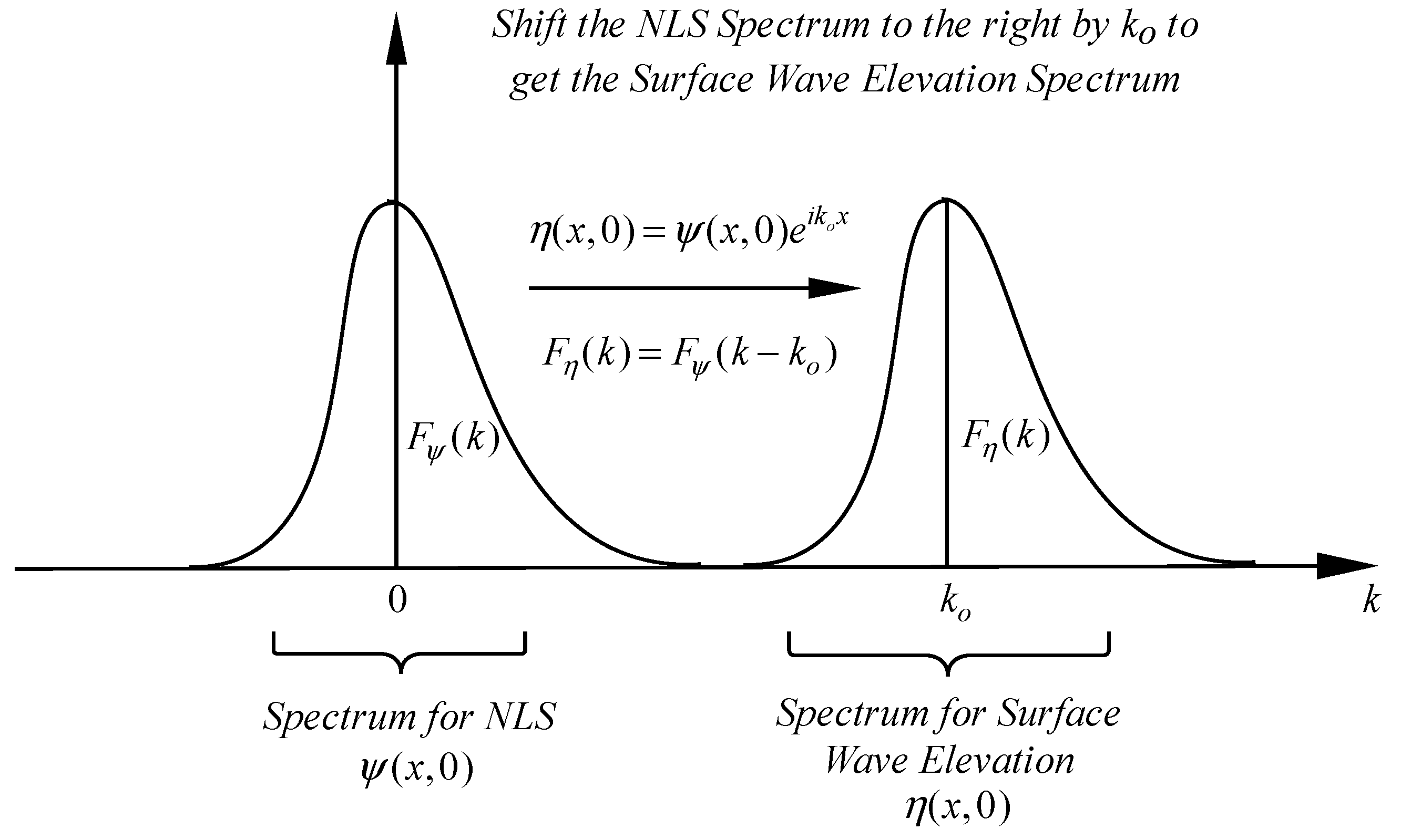
It is worth noting that (14) can be interpreted in terms of the Fourier shifting theorem. The real part of (14) is the measured (in an experimental context) surface wave elevation (11). Let us now see the physics of the shifting theorem. The complex modulation envelope is given by $\psi (x,0)$ and its spectrum is centered about zero modulational wavenumber K = K’ ≈ 0 and frequency $\Omega ={\Omega }^{\prime }=\nu a_o^2<<1$: Thus the spectrum of $\psi (x,0)$, which we call $F_{\psi }(k)$, will be centered about the origin (Figure 1). The complex surface elevation $\eta (x,0)$ has Fourier spectrum $F_{\eta }(k)$ that is centered about wavenumber $k=k_o$ (and frequency $\omega ={\omega }_o$). Here the surface elevation wavenumber is $k=k_o\pm K$ and the frequency is $\omega ={\omega }_o\pm \Omega$. While we deal with the standard Fourier spectrum in this simple example in Figure 1, it is important to note that in what follows we will be physically dealing with quasiperiodic Fourier series and their spectrum on a discretuum of wavenumbers $n·K$ and frequencies $n·\mathbf{\Omega }$ (the discussion below describes this notation). It follows that perhaps the most important feature of this theoretical formulation is the characterization of the coherent structures by the Riemann spectrum $[\mathsf{\tau }$, ${\mathsf{\varphi }}^{-}$, ${\mathsf{\varphi }}^{+}$] of Stokes waves and breathers, not the sine wave amplitudes of standard Fourier series.

Furthermore, in terms of the theta functions, the quasiperiodic solution of NLS (8) tells us that we are guaranteed to find the Stokes corrections $K^{\prime }$ and ${\Omega }^{\prime }$ (the algebraic geometric formulas are given in the literature [3,39]), so that we have the particular wavenumbers and frequencies $k_o\pm (K+K^{\prime })$ and ${\omega }_o\pm (\Omega +{\Omega }^{\prime })$ for the surface elevation (11). These definitions are made clearer below in terms of quasiperiodic Fourier series. However, as discussed in Osborne et al. [1], these parameters can be obtained directly from the time series when analyzing data.

It is worthwhile noting that (8), in the absence of a modulation, has $K^{\prime }=0, \hspace{0.17em}{\Omega }^{\prime }=-\nu a_o^2=-{\omega }_o{k}_o^2{a}_o^2/2$ (the deep water case), and this provides the important plane wave solution of NLS:

$$\psi (x,t)=a_o{e}^{i{K}^{\prime }x-i{\Omega }^{\prime }t}=a_o{e}^{-i\nu a_o^{2}t}=a_o{e}^{-\frac{i}{2}{\omega }_o{k}_o^2{a}_o^{2}t}$$

(15)

The corresponding associated surface wave elevation (10) is

$$\eta (x,t)=a_o\cos \left[k_{o}x-{\omega }_o\left(1+k_o^2{a}_o^2/2\right)t\right]+\dots$$

Clearly this is the first term in the Stokes wave expansion, here given with the nonlinear Stokes deep water, amplitude-dependent correction first found in his fundamental paper over 170 years ago [47].

3. Quasiperiodic Fourier Series Solution of the NLS Equation and other Considerations

3.1. The Quasiperiodic Fourier Series

Consider the FGT solution of NLS (4):

$$\psi (x,t)=a_o\frac{\theta (x,t|\mathsf{\tau },{\mathsf{\varphi }}^{-})}{\theta (x,t|\mathsf{\tau },{\mathsf{\varphi }}^{+})}{e}^{i{K}^{\prime }x-i{\Omega }^{\prime }t}$$

(8)

The principle idea given in this paper, consistent with the Baker-Mumford theorem (see Appendix A and [4]) is to convert (8) to a quasiperiodic Fourier series (2). Once we have the quasiperiodic Fourier series, we can do all the new kinds of wonderful analytical and numerical computations possible with such a series. The Baker-Mumford theorem means that there must exist a quasiperiodic Fourier series for (8) which I write in the following form:

$$\psi (x,t)=a_o\frac{\theta (x,t|\mathsf{\tau },{\mathsf{\varphi }}^{-})}{\theta (x,t|\mathsf{\tau },{\mathsf{\varphi }}^{+})}{e}^{i{K}^{\prime }x-i{\Omega }^{\prime }t}={\displaystyle \sum _{n\in {\mathbf{\mathbb{Z}}}^N}{\psi }_n}{e}^{i(n·K+K^{\prime })x-i(n·\mathbf{\Omega }+{\Omega }^{\prime })t+in·\Phi }$$

(16)

The goal is to find the coefficients ${\psi }_n$, the frequencies $\mathbf{\Omega }$ and phases $\Phi$ to make (16) true. I now carry out this computation, based on an idea of Zygmund [48].

First, we write the theta functions in terms of their usual definition as a quasiperiodic Fourier series [49,50,51]:

$$\theta (x,t|\mathsf{\tau },\hspace{0.17em}\hspace{0.17em}{\mathsf{\varphi }}^{\mp })={\displaystyle \sum _{n\in {\mathbf{\mathbb{Z}}}^N}{\theta }_n}{e}^{in·K\hspace{0.17em}x-in·\mathbf{\Omega }\hspace{0.17em}t+in·{\mathsf{\varphi }}^{\mp }},\hspace{0.17em}\hspace{0.17em}\hspace{0.17em}\hspace{0.17em}\hspace{0.17em}{\theta }_n=e^{\pi i\hspace{0.17em}n·\mathsf{\tau }\hspace{0.17em}n}$$

(17)

Notice that I have used the modulational wavenumbers $K$ and modulational frequencies $\mathbf{\Omega }$ in this expression. This is because the solution of NLS is always in terms of these parameters, i.e., those for the modulations (for which I use the capital symbols $K$ and $\mathbf{\Omega }$ as in Yuen and Lake [41]), not for the surface elevation (for which I use $k$ and $\mathsf{\omega }$). Here, $\mathsf{\tau }$ is the period matrix that contains the Riemann spectrum of the quasiperiodic modulations: This matrix contains Stokes waves on the diagonal elements and the breathers consist of two-by-two sub matrices along the diagonal with appropriate dynamical phases (this is essentially the phase locking of two Stokes waves to obtain a breather [3]). There are two sets of the phases, one for the numerator ${\mathsf{\varphi }}^{-}$ and one for the denominator ${\mathsf{\varphi }}^{+}$ (see Tracy and Chen [39] and Osborne [3] for formulas to compute these parameters).

I now absorb the phases into the coefficients, i.e., rewrite (17) in the following way:

$$\theta (x,t|\mathsf{\tau },\hspace{0.17em}\hspace{0.17em}{\mathsf{\varphi }}^{\mp })={\displaystyle \sum _{n\in {\mathbf{\mathbb{Z}}}^N}{\theta }_n^{\mp }}{e}^{in·Kx-in·\Omega t},\hspace{0.17em}\hspace{0.17em}\hspace{0.17em}\hspace{0.17em}\hspace{0.17em}\hspace{0.17em}\hspace{0.17em}\hspace{0.17em}\hspace{0.17em}\hspace{0.17em}{\theta }_n^{\mp }={\theta }_n{e}^{in·{\mathsf{\varphi }}^{\mp }}=e^{\pi in·\mathsf{\tau }\hspace{0.17em}n+in·{\mathsf{\varphi }}^{\mp }}$$

(18)

let us compute the ratio $R(x,t|\mathsf{\tau },{\mathsf{\varphi }}^{-},{\mathsf{\varphi }}^{+})$ of the two theta functions in (16) as a quasiperiodic Fourier series:

$$R(x,t|\mathsf{\tau },{\mathsf{\varphi }}^{-},{\mathsf{\varphi }}^{+})=\frac{\theta (x,t|{\mathsf{\varphi }}^{-})}{\theta (x,t|{\mathsf{\varphi }}^{+})}=\theta (x,t|{\mathsf{\varphi }}^{-}){\theta }^{-1}(x,t|{\mathsf{\varphi }}^{+})={\displaystyle \sum _{n\in {\mathbf{\mathbb{Z}}}^N}{R}_n}{e}^{in·Kx-in·\Omega t}$$

(19)

Note that I have suppressed the $\mathsf{\tau }$ in the theta functions for simplicity. The fact that such a result exists is justified by the Baker-Mumford theorem (see Appendix A), which states (in part) that a single valued, multiperiodic, meromorphic Fourier series can be found from the ratio of two theta functions with different phases. The Baker-Mumford theorem does not give a procedure for determining the quasiperiodic Fourier series. The construction of the right hand series in (19) is a goal of this paper. FGT theory tells us how to connect the parameters of the theta functions (period matrix, frequencies and phases) to a particular Cauchy or boundary value problem [6,39]. The solution to the NLS equation then has the form

$$\psi (x,t)=a_o\frac{\theta (x,t|{\mathsf{\varphi }}^{-})}{\theta (x,t|{\mathsf{\varphi }}^{+})}{e}^{i{K}^{\prime }x-i{\Omega }^{\prime }t}=a_o{\displaystyle \sum _{n\in {\mathbf{\mathbb{Z}}}^N}{R}_n}{e}^{i(n·K+K^{\prime })x-i(n·\mathbf{\Omega }+{\Omega }^{\prime })t}$$

(20)

To compute the series in (19), we first need to compute the inverse series of the denominator, which we define to be

$$Q(x,t|{\mathsf{\varphi }}^{+})=\frac{1}{\theta (x,t|{\mathsf{\varphi }}^{+})}={\theta }^{-1}(x,t|{\mathsf{\varphi }}^{+})={\displaystyle \sum _{n\in {\mathbf{\mathbb{Z}}}^N}{Q}_n^{+}}{e}^{in·Kx-in·\Omega t}$$

(21)

where $Q_n^{+}$ are the coefficients of the series (21) which we call an inverse theta function series. The $Q_n^{+}$ are determined by a method of Zygmund [48] for ordinary Fourier series, but which is here applied to multiperiodic Fourier series. We have $Q(x,t|{\mathsf{\varphi }}^{+})=1/\theta (x,t|{\mathsf{\varphi }}^{+}),$ so that $\theta (x,t|{\mathsf{\varphi }}^{+})\hspace{0.17em}Q(x,t|{\mathsf{\varphi }}^{+})=1,$ implying a convolution for the coefficients of the product $\theta (x,t|{\mathsf{\varphi }}^{+})\hspace{0.17em}Q(x,t|{\mathsf{\varphi }}^{+}):$

$$\theta (x,t|{\mathsf{\varphi }}^{+})Q(x,t|{\mathsf{\varphi }}^{+})={\displaystyle \sum _{n\in {\mathbf{\mathbb{Z}}}^N}{\delta }_n{e}^{in·Kx-in·\Omega t}}=1$$

so that

$${\displaystyle \sum _{m\in {\mathbf{\mathbb{Z}}}^N}{\theta }_{n-m}^{+}{Q}_m^{+}={\delta }_n},\hspace{0.17em}\hspace{0.17em}\hspace{0.17em}\hspace{0.17em}\hspace{0.17em}\hspace{0.17em}\hspace{0.17em}\hspace{0.17em}\hspace{0.17em}\hspace{0.17em}\hspace{0.17em}\hspace{0.17em}\hspace{0.17em}\hspace{0.17em}\mathsf{\delta }=\{{\delta }_n\}=\left[\begin{array}{c}⋮\\ 0\\ 1\\ 0\\ ⋮\end{array}\right]$$

(22)

Note that the definition of ${\delta }_n$ is:

$${\delta }_n=\{\begin{array}{c}1 \mathrm{if} n=0\\ 0 \mathrm{if} n\ne 0\end{array}$$

To be clear, we have from (18) and (21) the quasiperiodic Fourier series with the coefficients ${\theta }_n^{+}$ and $Q_n^{+}$:

$$\begin{gathered} \theta (x,t|{\mathsf{\varphi }}^{+})={\displaystyle \sum _{n\in {\mathbf{\mathbb{Z}}}^N}{\theta }_n^{+}}{e}^{i\hspace{0.17em}n·Kx-i\hspace{0.17em}n·\Omega t}, {\theta }_n^{+}={\theta }_n{e}^{in·{\mathsf{\varphi }}^{+}}=e^{\pi i\hspace{0.17em}n·\mathsf{\tau }\hspace{0.17em}n+i\hspace{0.17em}n·{\mathsf{\varphi }}^{+}} \\ Q(x,t|{\mathsf{\varphi }}^{+})={\displaystyle \sum _{n\in {\mathbf{\mathbb{Z}}}^N}{Q}_n^{+}}{e}^{in·Kx-in·\Omega t} \end{gathered}$$

(23)

In matrix-vector notation, we have ${\tilde{\mathsf{\theta }}}^{+}{\mathbf{Q}}^{+}=\mathsf{\delta }$ for (22). By definition, ${\mathbf{Q}}^{+}=\{Q_n\}$ is an unknown infinite length column vector and ${\mathsf{\theta }}^{+}=\{{\theta }_{n-m}^{+}\}$ is an infinite dimensional matrix formed from the known coefficients on the right hand side of the first line of Equation (23):

$${\theta }_{n-m}^{+}={\theta }_{n-m}{e}^{i(n-m)·\hspace{0.17em}{\mathsf{\varphi }}^{+}}=e^{\pi i(n-m)·\hspace{0.17em}\mathsf{\tau }(n-m)+i(n-m)·\hspace{0.17em}{\mathsf{\varphi }}^{+}}$$

(24)

${\mathbf{Q}}^{+}=\{Q_n^{+}\}$ is a vector we seek in terms of the Riemann spectrum $\{\mathsf{\tau },\hspace{0.17em}\hspace{0.17em}{\mathsf{\varphi }}^{+}\}$. This leads to the vector of coefficients $Q^{+}={({\mathsf{\theta }}^{+})}^{-1}\mathsf{\delta }$ of the inverse series (21). Here, $\mathsf{\delta }$ is an infinite length column vector whose elements are all zero except for that at the central position, that is 1, i.e., for which $n=0$. In this way, $\mathsf{\delta }$ is just the unit one, $\mathsf{\delta }=1.$ In component form, we have from (22)

$$\{\hspace{0.17em}{Q}_n^{+}\}={\{{\theta }_{n-m}^{+}\}}^{-1}\{{\delta }_m\}$$

(25a)

The convergence of the series (16, 17, 21, 23) occurs because of the extraordinary properties of theta functions [6,49,50,51,52,53]. In this way, one is led to the conclusion that the matrix ${\tilde{\mathsf{\theta }}}^{+}=\{{\theta }_{n-m}^{+}\}$ is invertible (see also Zygmund [48] for arguments relating to the convergence properties).

Now we have the coefficients we seek from (25a):

$$Q_n^{+}={\displaystyle \sum _{m\in {\mathbf{\mathbb{Z}}}^N}{[{\theta }_{n-m}^{+}]}^{-1}{\delta }_m}$$

(25b)

which then can be explicitly written

$$Q_n^{+}\equiv {\theta }_n^{-1}={\displaystyle \sum _{m\in {\mathbf{\mathbb{Z}}}^N}{[e^{\pi i(n-m)·\hspace{0.17em}\mathsf{\tau }(n-m)+i(n-m)·\hspace{0.17em}{\mathsf{\varphi }}^{+}}]}^{-1}}{\mathsf{\delta }}_m$$

(26)

Now we need to complete the computation of (19)

$$R(x,t|{\mathsf{\varphi }}^{-},{\mathsf{\varphi }}^{+})=\theta (x,t|{\mathsf{\varphi }}^{-})Q(x,t|{\mathsf{\varphi }}^{+})={\displaystyle \sum _{n\in {\mathbf{\mathbb{Z}}}^N}{R}_n}{e}^{in·Kx-in·\Omega t}$$

(27)

where

$$\begin{gathered} \theta (x,t|{\mathsf{\varphi }}^{-})={\displaystyle \sum _{n\in {\mathbf{\mathbb{Z}}}^N}{\theta }_n^{-}}{e}^{in·Kx-in·\Omega t}, {\theta }_n^{-}={\theta }_n{e}^{in·{\mathsf{\varphi }}^{-}}=e^{\pi in·\mathsf{\tau }\hspace{0.17em}n+in·{\mathsf{\varphi }}^{-}} \\ Q(x,t|{\mathsf{\varphi }}^{+})={\displaystyle \sum _{n\in {\mathbf{\mathbb{Z}}}^N}{Q}_n^{+}}{e}^{in·Kx-in·\Omega t}, \hspace{0.17em}{Q}_n^{+}={\displaystyle \sum _{m\in {\mathbf{\mathbb{Z}}}^N}{[e^{\pi i(n-m)·\hspace{0.17em}\mathsf{\tau }\hspace{0.17em}(n-m)+i(n-m)·\hspace{0.17em}{\mathsf{\varphi }}^{+}}]}^{-1}}{\mathsf{\delta }}_m \end{gathered}$$

(28)

Equation (27) implies a convolution of the coefficients given explicitly in terms of the Riemann spectrum (the amplitudes and phases of FGT: $[\mathsf{\tau },\hspace{0.17em}\hspace{0.17em}{\mathsf{\varphi }}^{-},\hspace{0.17em}\hspace{0.17em}{\mathsf{\varphi }}^{+}]$) in (27). Let us now write this convolution.

For the product of two Fourier series $A(x,t),\hspace{0.17em}\hspace{0.17em}B(x,t)$ we define:

$$\begin{gathered} A(x,t)={\displaystyle \sum _{n\in {\mathbf{\mathbb{Z}}}^N}{A}_n}{e}^{in·K\hspace{0.17em}x-in·\Omega \hspace{0.17em}t} \\ B(x,t)={\displaystyle \sum _{n\in {\mathbf{\mathbb{Z}}}^N}{B}_n}{e}^{in·K\hspace{0.17em}x-in·\Omega \hspace{0.17em}t} \end{gathered}$$

Then the product is

$$C(x,t)=A(x,t)B(x,t)={\displaystyle \sum _{n\in {\mathbf{\mathbb{Z}}}^N}{C}_n}{e}^{in·K\hspace{0.17em}x-in·\Omega \hspace{0.17em}t}$$

We use the well-known result [48]:

$$C_n={\displaystyle \sum _{m\hspace{0.17em}\in {\mathbf{\mathbb{Z}}}^N}{A}_m{B}_{n-m}}={\displaystyle \sum _{m+l=n\hspace{0.17em}\in \hspace{0.17em}{\mathbf{\mathbb{Z}}}^N}{A}_m{B}_l}$$

Both ways to write this latter expression are equivalent: The first is a convolution, while the second describes three-wave interactions. Finally we have

$$R_i={\displaystyle \sum _{j\hspace{0.17em}\in {\mathbf{\mathbb{Z}}}^N}{\theta }_{i-j}^{-}{Q}_j^{+}}={\displaystyle \sum _{j+l=n\hspace{0.17em}\in \hspace{0.17em}{\mathbf{\mathbb{Z}}}^N}{Q}_j^{+}{\theta }_l^{-}}$$

where

$${\theta }_n^{-}={\theta }_n{e}^{i\hspace{0.17em}n·\hspace{0.17em}{\mathsf{\varphi }}^{-}}=e^{\pi i\hspace{0.17em}n·\hspace{0.17em}\mathsf{\tau }n+i\hspace{0.17em}n·\hspace{0.17em}{\mathsf{\varphi }}^{-}}$$

Then

$${\theta }_{n-m}^{-}={\theta }_{n-m}{e}^{i(n-m)·\hspace{0.17em}{\mathsf{\varphi }}^{-}}=e^{\pi i(n-m)·\hspace{0.17em}\mathsf{\tau }(n-m)+i(n-m)·\hspace{0.17em}{\mathsf{\varphi }}^{-}}$$

The following are then the results of the convolution:

$$\begin{gathered} \boxed{R_n(\mathsf{\tau },{\mathsf{\varphi }}^{+},{\mathsf{\varphi }}^{-})={\displaystyle \sum _{m\in {\mathbf{\mathbb{Z}}}^N}{Q}_m^{+}{\theta }_{n-m}^{-}}={\displaystyle \sum _{m\in {\mathbf{\mathbb{Z}}}^N}{\theta }_m^{-1}{\theta }_{n-m}^{-}}={\displaystyle \sum _{m\in {\mathbf{\mathbb{Z}}}^N}{\theta }_{n-m}^{-}{\theta }_m^{-1}} \\ {Q}_n^{+}={\theta }_n^{-1}={\displaystyle \sum _{m\in {\mathbf{\mathbb{Z}}}^N}{[e^{\pi i(n-m)·\hspace{0.17em}\mathsf{\tau }(n-m)+i(n-m)·\hspace{0.17em}{\mathsf{\varphi }}^{+}}]}^{-1}}{\mathsf{\delta }}_m \\ {\theta }_{n-m}^{-}={\theta }_m{e}^{i(n-m)·\hspace{0.17em}{\mathsf{\varphi }}^{-}}=e^{\pi i(n-m)·\hspace{0.17em}\mathsf{\tau }(n-m)+i(n-m)·{\mathsf{\varphi }}^{-}}} \end{gathered}$$

(29a)

Or, simplifying the notation:

$$\boxed{\begin{array}{l}{R}_n(\mathsf{\tau },{\mathsf{\varphi }}^{+},{\mathsf{\varphi }}^{-})={\displaystyle \sum _{m\in {\mathbf{\mathbb{Z}}}^N}{\theta }_{n-m}^{-}{\theta }_m^{-1}}\\ \hspace{0.17em}\hspace{0.17em}\hspace{0.17em}\hspace{0.17em}\hspace{0.17em}\hspace{0.17em}\hspace{0.17em}\hspace{0.17em}\hspace{0.17em}\hspace{0.17em}{\theta }_{n-m}^{-}=e^{\pi i(n-m)·\mathsf{\tau }(n-m)+i(n-m)·\hspace{0.17em}{\mathsf{\varphi }}^{-}}\hspace{0.17em}\\ \hspace{0.17em}\hspace{0.17em}\hspace{0.17em}\hspace{0.17em}\hspace{0.17em}\hspace{0.17em}\hspace{0.17em}\hspace{0.17em}\hspace{0.17em}\hspace{0.17em}{\theta }_n^{-1}={\displaystyle \sum _{m\in {\mathbf{\mathbb{Z}}}^N}{[e^{\pi i(n-m)·\hspace{0.17em}\mathsf{\tau }(n-m)+i(n-m)·\hspace{0.17em}{\mathsf{\varphi }}^{+}}]}^{-1}}{\mathsf{\delta }}_m\end{array}}$$

(29b)

The latter expressions can also be written in the following form:

$$\boxed{\begin{array}{l}{R}_n(\mathsf{\tau },{\mathsf{\varphi }}^{+},{\mathsf{\varphi }}^{-})={\displaystyle \sum _{j\in {\mathbf{\mathbb{Z}}}^N}{A}_{n\hspace{0.17em}\hspace{0.17em}-j}(\mathsf{\tau },{\mathsf{\varphi }}^{-}){\displaystyle \sum _{m\in {\mathbf{\mathbb{Z}}}^N}{[A_{\hspace{0.17em}j\hspace{0.17em}-m}(\mathsf{\tau },{\mathsf{\varphi }}^{+})]}^{-1}}{\mathsf{\delta }}_m}\\ \hspace{0.17em}\hspace{0.17em}\hspace{0.17em}\hspace{0.17em}\hspace{0.17em}\hspace{0.17em}\hspace{0.17em}\hspace{0.17em}\hspace{0.17em}\hspace{0.17em}\hspace{0.17em}\hspace{0.17em}{A}_n(\mathsf{\tau },\mathsf{\varphi })=e^{\pi in·\mathsf{\tau }\hspace{0.17em}n+in·\mathsf{\varphi }}\end{array}}$$

(29c)

These are the coefficients $R_n(\mathsf{\tau },{\mathsf{\varphi }}^{+},{\mathsf{\varphi }}^{-})$ on the right hand side of the series (20). We have thus found the quasiperiodic Fourier series for the solution of the NLS equation, as originally sought. Notice that Equations (20) retain the same information as the theta function formulation of the solution of the NLS equation as a ratio of Riemann theta functions (20), namely the period matrix $\mathsf{\tau }$, and phases $({\mathsf{\varphi }}^{+},{\mathsf{\varphi }}^{-})$ describing the Cauchy initial conditions. One can choose which of the three forms of the coefficients (29) is appropriate for a particular application. To help see what I mean, I give a simple example in Section 3.2.

In summary, the quasiperiodic solution to the NLS equation then has two equivalent forms: (1) the ratio of two Riemann theta functions with different phases and (2) a quasiperiodic Fourier series.

$$\psi (x,t)=a_o\frac{\theta (x,t|{\mathsf{\varphi }}^{-})}{\theta (x,t|{\mathsf{\varphi }}^{+})}{e}^{i{K}^{\prime }x-i{\Omega }^{\prime }t}={\displaystyle \sum _{n\in {\mathbf{\mathbb{Z}}}^N}{\psi }_n}{e}^{i(n·\hspace{0.17em}K+K^{\prime }\hspace{0.17em})x-i(n·\hspace{0.17em}\mathbf{\Omega }+{\Omega }^{\prime })t}$$

(30)

where the Stokes wave corrections $K^{\prime }$ and ${\Omega }^{\prime }$ are given in the Appendix A of Tracy and Chen [39]. Here, as discussed above, to determine (30), the coefficients are given by ${\psi }_n=a_o{R}_n(\mathsf{\tau },{\mathsf{\varphi }}^{-},{\mathsf{\varphi }}^{+})$ plus any of the equivalent forms of (29).

3.2. An Approximation for a Single Degree of Freedom Solution

I now give some insight about the coefficients in (29) and how to compute them. Here is the matrix we need to invert, that depends on the period matrix $\mathsf{\tau }$ and phase $\mathsf{\varphi }$:

$$A_{ij}(\mathsf{\tau },\mathsf{\varphi })=e^{\pi i(i-j)·\hspace{0.17em}\mathsf{\tau }(i-j)+i(i-j)·\hspace{0.17em}\mathsf{\varphi }}$$

(31)

Clearly $i\in {\mathbf{\mathbb{Z}}}^N$ and $j\in {\mathbf{\mathbb{Z}}}^N.$ The full generality and associated computations of the algebra of matrices, whose indices are two infinite-length integer vectors i and j, will be explored in a future paper. For now, let us look at the genus 1 case where we have a period matrix $\tau$ which is 1 × 1, a simple complex number. Then sum from −1, 0, 1 (essentially the first two terms in the Stokes wave) for each of the two indices i and j, so that the infinite matrix is reduced to a 3 × 3 case:

$$\begin{gathered} A{\hspace{0.17em}}_{ij}(q,\varphi )=q^{{(i-j)}^2}{e}^{i(i-j)\hspace{0.17em}\varphi }, \hspace{0.17em}q=e^{\pi i\tau } \\ \{A_{ij}(q,\varphi )\}=\left[\begin{array}{ccc}1& q{e}^{-i\varphi }& q^4{e}^{-2i\varphi }\\ q{e}^{i\varphi }& 1& q{e}^{-i\varphi }\\ q^4{e}^{i2\varphi }& q{e}^{i\varphi }& 1\end{array}\right] \end{gathered}$$

(32)

One might query at this point why we can deal physically with a 3 × 3 matrix when in reality the matrix is infinitely dimensional. In the present simple case, we assume that $|q|<<1$, so the resultant three term Stokes series is defined by $|q|<<1$. Then the inverse is

$$\{A_{ij}^{-1}(q,\varphi )\}=\frac{1}{{(1-q^2)}^3(1+q^2)}\left[\begin{array}{ccc}1-q^2& -q{e}^{-i\varphi }(1-q^4)& q^2{e}^{-i\varphi }(1-q^2)\\ -q{e}^{i\varphi }(1-q^4)& 1-q^8& -q{e}^{-i\varphi }(1-q^4)\\ q^2{e}^{i\varphi }(1-q^2)& -q{e}^{i\varphi }(1-q^4)& 1-q^2\end{array}\right]$$

According to (29), we need the central column vector of this latter matrix:

$$\{V_k(q,\varphi )\}=\{A_{kj}^{-1}(q,\varphi )\}\{{\delta }_j\}=\frac{1}{{(1-q^2)}^3(1+q^2)}\left[\begin{array}{c}-q{e}^{-i\varphi }(1-q^4)\\ 1-q^8\\ -q{e}^{i\varphi }(1-q^4)\end{array}\right]$$

Now evaluate this to order $q$ and use the “plus“ phase

$$\{V_k(q,{\varphi }^{+})\}=\{A_{kj}^{-1}(q,{\varphi }^{+})\}\{{\delta }_j\}\sim \left[\begin{array}{c}-q{e}^{-i{\varphi }^{+}}\\ 1\\ -q{e}^{i{\varphi }^{+}}\end{array}\right]$$

(33)

Multiply this result times the $A$ matrix (29c) with the negative phase:

$$\begin{array}{ll}\{R_i(q,{\varphi }^{+},{\varphi }^{-})\}& =\{A_{ik}(q,{\varphi }^{-})\}\{A_{kj}^{-1}(q,{\varphi }^{+})\}\{{\delta }_j\}\hspace{0.17em}\\ & =\left[\begin{array}{ccc}1& q{e}^{-i{\varphi }^{-}}& 0\\ q{e}^{i{\varphi }^{-}}& 1& q{e}^{-i{\varphi }^{-}}\\ 0& q{e}^{i{\varphi }^{-}}& 1\end{array}\right]\left[\begin{array}{c}-q{e}^{-i{\varphi }^{+}}\\ 1\\ -q{e}^{i{\varphi }^{+}}\end{array}\right]\end{array}$$

These then are the coefficients of the quasiperiodic Fourier series

$$\hspace{0.17em}\{R_n(q,{\varphi }^{+},{\varphi }^{-})\}=\{A_{nk}(q,{\varphi }^{-})\}\{A_{kj}^{-1}(q,{\varphi }^{+})\}\{{\delta }_j\}=\left[\begin{array}{c}q\left(e^{-i{\varphi }^{-}}-e^{-i{\varphi }^{+}}\right)\\ 1\\ q\left(e^{i{\varphi }^{-}}-e^{i{\varphi }^{+}}\right)\end{array}\right]$$

(34)

Now from (30) we seek the first three terms in the one-degree-of-freedom solution of NLS:

$$\psi (x,t)=a_o\frac{\theta (x,t|{\varphi }^{-})}{\theta (x,t|{\varphi }^{+})}{e}^{i{K}^{\prime }x-i{\Omega }^{\prime }t}=a_o{\displaystyle \sum _{n=-1}^1{R}_n{e}^{i(K_n+K^{\prime })x-i({\Omega }_n+{\Omega }^{\prime })t}}$$

This gives

$$\begin{array}{ll}\psi (x,t)& =a_{o}q\left(e^{-i{\varphi }^{-}}-e^{-i{\varphi }^{+}}\right)e^{i(K_{-1}+K^{\prime })x-i({\Omega }_{-1}+{\Omega }^{\prime })t}+a_o{e}^{i(K_o+K^{\prime })x-i({\Omega }_o+{\Omega }^{\prime })t}\\ & +a_{o}q\left(e^{i{\varphi }^{-}}-e^{i{\varphi }^{+}}\right)e^{i(K_1+K^{\prime })x-i({\Omega }_1+{\Omega }^{\prime })t}\end{array}$$

If we use the familiar physical Stokes correction for a single degree of freedom $K^{\prime }=0,\hspace{0.17em}\hspace{0.17em}\hspace{0.17em}{\Omega }^{\prime }=\nu a_o^2$ and further simplify by setting ${{\rm K}}_{-1}=-{\rm K}$, ${{\rm K}}_1={\rm K}$, ${\Omega }_{\hspace{0.17em}-1}=-\Omega$ and ${\Omega }_1=\Omega$ so that we find (see Figure 2):

$$\psi (x,t)=a_{o}q\left(e^{-i{\varphi }^{-}}-e^{-i{\varphi }^{+}}\right)e^{-iKx+i(\Omega -\nu a_o^2)t}+a_o{e}^{-i\nu a_o^{2}t}+a_{o}q\left(e^{i{\varphi }^{-}}-e^{i{\varphi }^{+}}\right)e^{iKx-i(\Omega +\nu a_o^2)t}$$

or

$$\psi (x,t)=a_o{e}^{-i\nu a_o^{2}t}+{\epsilon }_{-}{e}^{-iKx+i(\Omega -\nu a_o^2)t}+{\epsilon }_{+}{e}^{iKx-i(\Omega +\nu a_o^2)t}$$

(35)

where

$$\begin{array}{l}{\epsilon }_{-}=a_{o}q\left(e^{-i{\varphi }^{-}}-e^{-i{\varphi }^{+}}\right)\\ {\epsilon }_{+}= a_{o}q\left(e^{i{\varphi }^{-}}-e^{i{\varphi }^{+}}\right)\end{array}$$

(36)

Notice that if ${\varphi }^{-}=0,\hspace{0.17em}{\varphi }^{+}=\pi$, then:

$${\epsilon }_{-}={\epsilon }_{+}=\hspace{0.17em}\hspace{0.17em}2a_{o}q$$

This latter result is the case of a dnoidal wave solution of the NLS equation, which is of course stable (see discussion below in Section 3.5). Otherwise we are more interested in the general case just derived (35) where the phases are arbitrary so that instabilities can occur and we write (35):

$$\psi (x,t)=\left[a_o+{\epsilon }_{-}{e}^{-iKx+i\Omega t}+{\epsilon }_{+}{e}^{iKx-i\Omega t}\right]e^{-i\nu a_o^{2}t}$$

(37)

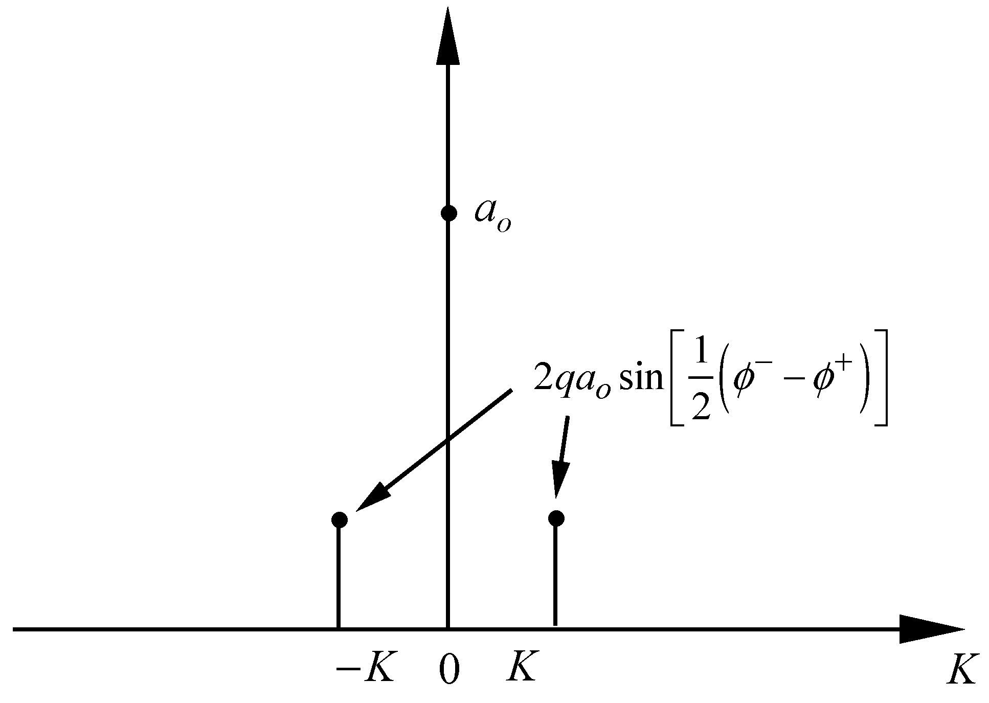
This is the starting place of Yuen and Lake [41] who derived the modulational dispersion relation by inserting this expression into the NLS equation and linearizing about $a_o$ and solving the resultant eigenvalue problem for ${\epsilon }_{-}$ and ${\epsilon }_{+}$ (see Section 3.4 below for details). The above expression (37), derived here from the quasiperiodic Fourier series solution of the NLS Equation (30), can of course be generalized to arbitrary order and to an arbitrary number of degrees of freedom using the methods just discussed. Likewise, the modulational dispersion relation can be derived to arbitrary order, which is necessary for the analysis of measured time series (see discussion below in Section 3.4). The spectrum of the small amplitude modulation (37) is given in Figure 2.

The complex surface elevation associated with (37) is

$$\begin{array}{ll}\Xi (x,t)& =\psi (x,t)e^{i{k}_{o}x-i{\omega }_{o}t}\\ & =a_o\hspace{0.17em}q\left(e^{-i{\varphi }^{-}}-e^{-i{\varphi }^{+}}\right)e^{i(k_o+K_{-1})\hspace{0.17em}-i({\omega }_o+{\Omega }_{-1}+\nu a_o^2)t}+a_o{e}^{i{k}_{o}x-i({\omega }_o+\nu a_o^2)t}\\ & +a_o\hspace{0.17em}q\left(e^{i{\varphi }^{-}}-e^{i{\varphi }^{+}}\right)e^{i(k_o+K_1)x-i({\omega }_o+{\Omega }_1+\nu a_o^2)t}\end{array}$$

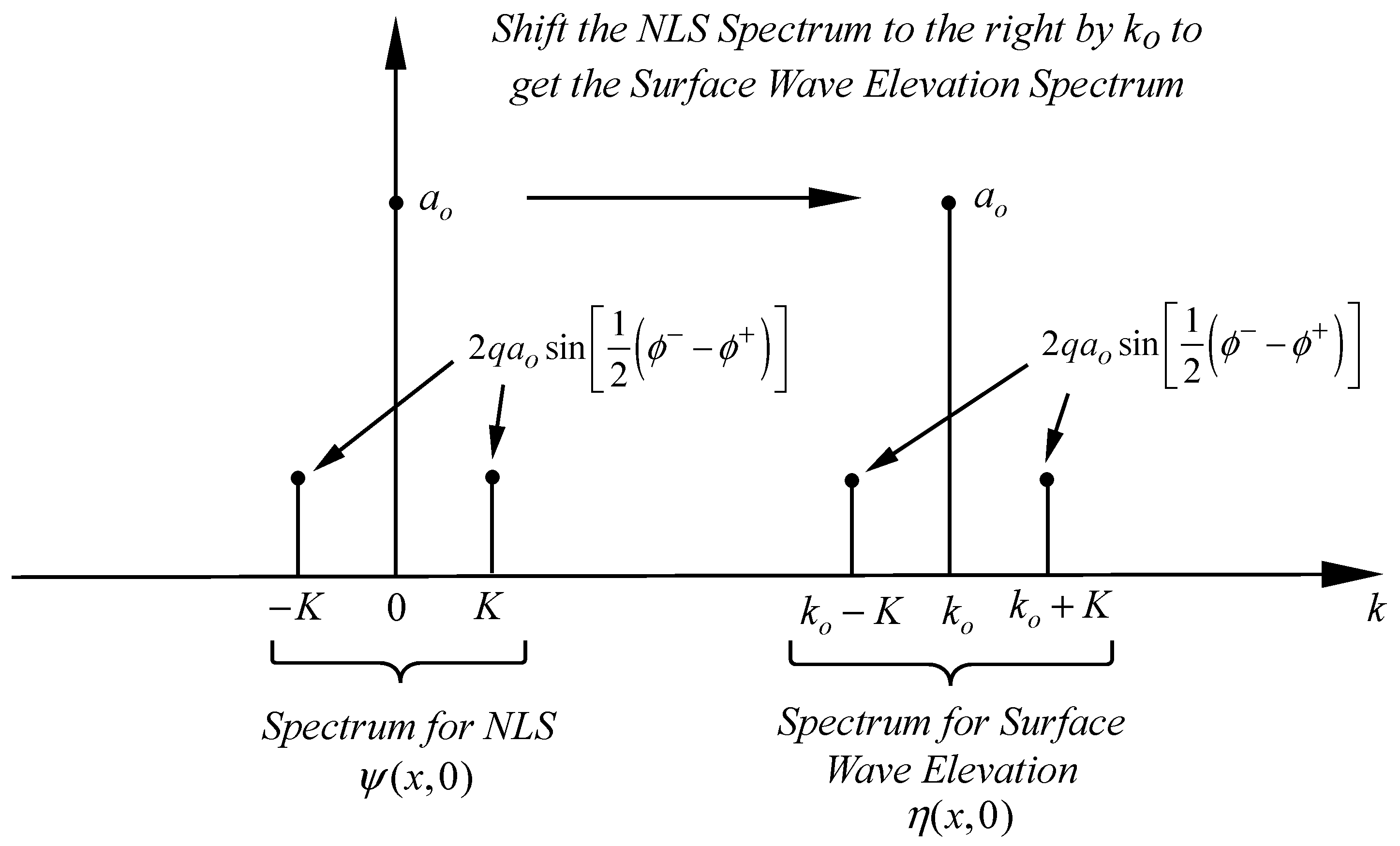
Taking the real part and simplifying as before (see the associated spectrum in Figure 3):

$$\begin{array}{ll}\eta (x,t)& =a_o\cos [k_{o}x-({\omega }_o+\nu a_o^2)t]\\ & +{\epsilon }_{-}\cos [(k_o-K)x-({\omega }_o-\Omega +\nu a_o^2)t]+{\epsilon }_{+}\cos [(k_o+K)x-({\omega }_o+\Omega +\nu a_o^2)t]\end{array}$$

(38)

Note that the dnoidal wave (Section 3.5 below) occurs when there is a difference of $\pi$ between the phases. So the general case has complex phases (see (48) below) and hence distinct epsilons ${\epsilon }_{-},\hspace{0.17em}\hspace{0.17em}{\epsilon }_{+}$ and therefore we have the generality necessary to obtain the modulational dispersion relation (Section 3.4).

3.3. Another Approximation for a Single Degree of Freedom Small Amplitude Solution

To approximately evaluate the above theta function solution (8) for the NLS equation for a single Stokes waves (genus 1) solution, let us first find the ratio of two theta functions with different phases out to order q in the elliptic nome:

$$\frac{\theta (x,t|{\varphi }_1)}{\theta (x,t|{\varphi }_2)}\simeq \frac{1+2q\cos \left(K\hspace{0.17em}x-\Omega t+{\varphi }^{-}\right)}{1+2q\cos \left(K\hspace{0.17em}x-\Omega t+{\varphi }^{+}\right)}$$

(39)

where $q=e^{\pi i\tau }$, for $\tau$ the single period matrix element. The next order terms are O($q^4$) and are not included at this simple stage of the analysis. This derivation compliments the results of the last Section 3.2 where the results are much more general. The derivation given here is much simpler, but insufficient for the case of arbitrary genus. We would like to get the leading order Fourier series for this ratio. The power series approximation to order q has the form:

$$\frac{1+2q\cos \left(K\hspace{0.17em}x-\Omega t+{\varphi }^{-}\right)}{1+2q\cos \left(K\hspace{0.17em}x-\Omega t+{\varphi }^{+}\right)}\simeq 1+2q\left[\cos \left(Kx-\Omega t+{\varphi }^{\_}\right)-\cos \left(Kx-\Omega t+{\varphi }^{+}\right)\right]$$

(40)

which leads to the simple expression

$$\frac{1+2q\cos \left(K\hspace{0.17em}x-\Omega t+{\varphi }^{\_}\right)}{1+2q\cos \left(K\hspace{0.17em}x-\Omega t+{\varphi }^{+}\right)}\simeq \hspace{0.17em}1-4q\sin \left[\frac{1}{2}\left({\varphi }^{\_}-{\varphi }^{+}\right)\right]\sin \left[Kx-\Omega t+\frac{1}{2}\left({\varphi }^{\_}+{\varphi }^{+}\right)\right]$$

(41)

This means that the leading order complex modulational solution of the NLS equation is (here I take the standard result $K^{\prime }=0$ and ${\Omega }^{\prime }=\nu a_o^2$, which is the Stokes frequency correction)):

$$\psi (x,t)\simeq a_o\left\{\hspace{0.17em}1-4q\sin \left[\frac{1}{2}\left({\varphi }^{-}-{\varphi }^{+}\right)\right]\sin \left[Kx-\Omega t+\frac{1}{2}\left({\varphi }^{-}+{\varphi }^{+}\right)\right]\right\}{e}^{i\nu a_o^{2}t}$$

(42)

And the surface wave elevation is:

$$\eta (x,t)=a_o\left\{\hspace{0.17em}1-4q\sin \left[\frac{1}{2}\left({\varphi }^{-}-{\varphi }^{+}\right)\right]\sin \left[Kx-\Omega t+\frac{1}{2}\left({\varphi }^{-}+{\varphi }^{+}\right)\right]\right\}\cos [k_{o}x-i({\omega }_o+\nu a_o^2)t]$$

(43)

We see that the surface elevation is a simple cosine (with the amplitude-dependent Stokes wave correction to the frequency included) with a small amplitude modulation (since $4a_{o}q\sin [({\varphi }_1-{\varphi }_2)/2]<<1$), which is long (since $K<<k_o$) and slowly varying (since $\Omega <<{\omega }_o$). Note that the amplitude of the modulation depends on the difference of the original phases, and the phase of the modulation depends on the sum of the original phases.

Now we write the above results in a more explicit form to enable us to graph the Fourier transform. Recall the relation:

$$\sin (x)=\frac{i}{2}\left(e^{-ix}-e^{ix}\right)$$

Use this in the above to find:

$$\frac{1+2q\cos \left(K\hspace{0.17em}x-\Omega t+{\varphi }^{-}\right)}{1+2q\cos \left(K\hspace{0.17em}x-\Omega t+{\varphi }^{+}\right)}\simeq \hspace{0.17em}1-2\epsilon \frac{i}{2}\left[e^{-iKx+i\Omega t-\frac{i}{2}({\varphi }^{-}+{\varphi }^{+})}-e^{iKx-i\Omega t+\frac{i}{2}({\varphi }^{-}+{\varphi }^{+})}\right]$$

(44)

for

$$\begin{gathered} i=e^{\frac{i}{2}\pi } \\ \epsilon =2q\sin \left[\frac{1}{2}\left({\varphi }^{-}-{\varphi }^{+}\right)\right] \\ {e}^{i\Phi }\equiv e^{i{\varphi }^{-}}-e^{i{\varphi }^{+}} \end{gathered}$$

The final result for the small amplitude solution of the NLS equation is:

$$\psi (x,t)=a_o{e}^{i{K}^{\prime }x-i{\Omega }^{\prime }t}+{\epsilon }_{-}{e}^{-i(K-K^{\prime })x+i(\Omega -{\Omega }^{\prime })t}+{\epsilon }_{+}{e}^{i(K+K^{\prime })x-i(\Omega +{\Omega }^{\prime })t}$$

(45)

where we set

$$\begin{gathered} {\epsilon }_{-}=a_{o}q{e}^{-i\Phi -i\pi /2} \\ {\epsilon }_{+}=a_{o}q{e}^{i\Phi +i\pi /2} \end{gathered}$$

Then we find

$$\begin{array}{l}{\epsilon }_{-}=2a_{o}q\sin \left[\frac{1}{2}\left({\varphi }^{-}-{\varphi }^{+}\right)\right]e^{-i({\varphi }^{-}+{\varphi }^{+})/2-i\pi /2}\\ {\epsilon }_{+}= \hspace{0.17em}{\epsilon }_{-}^{*}=2a_{o}q\sin \left[\frac{1}{2}\left({\varphi }^{-}-{\varphi }^{+}\right)\right]e^{i({\varphi }^{-}+{\varphi }^{+})/2+i\pi /2}\end{array}$$

(46)

Where the complex phase is defined by

$$e^{i\Phi }\equiv e^{i{\varphi }^{-}}-e^{i{\varphi }^{+}}=2\sin \left[\frac{1}{2}\left({\varphi }^{-}-{\varphi }^{+}\right)\right]e^{i({\varphi }^{-}+{\varphi }^{+})/2+i\pi /2}$$

(47)

so that

$$\Phi =\frac{{\varphi }^{-}+{\varphi }^{+}}{2}+\frac{\pi }{2}-i\ln \left\{2\sin \left[\left(\frac{{\varphi }^{-}-{\varphi }^{+}}{2}\right)\right]\right\}$$

(48)

The quasiperiodic Fourier series, together with quasiperiodic inverse scattering theory, generically have phases with real and imaginary parts (see below with regard to breather construction in Section 3.8). Here the real part is related to the sum of the IST phases and the imaginary part is related to the difference of the phases.

Therefore alternative forms for the epsilons are

$$\begin{array}{l}{\epsilon }_{-}=a_{o}q\left(e^{-i{\varphi }^{-}}-e^{-i{\varphi }^{+}}\right)e^{-i\pi /2}=a_{o}q{e}^{-i\Phi -i\pi /2}\\ {\epsilon }_{+}= a_{o}q\left(e^{i{\varphi }^{-}}-e^{i{\varphi }^{+}}\right)e^{i\pi /2}=a_{o}q{e}^{i\Phi +i\pi /2}\end{array}$$

where I have used the relation for the complex phase $\Phi$ (47). Note that if we set ${\varphi }^{-}=0$, ${\varphi }^{+}=\pi$ we get the leading order term in the dnoidal wave solution of the NLS equation (Section 3.5 below). I will revisit this relation below for the introduction of the $\Phi$ with regard to the nonlinear random phase approximation (Section 4.1 below). Because $\Phi$ has real and imaginary parts it has an important extended role in periodic inverse scattering theory with respect to the real phases of standard Fourier series.

As mentioned above, we take $K^{\prime }=0$ and ${\Omega }^{\prime }=\nu a_o^2$. Then we again get the leading order estimate for a small amplitude modulation of the nonlinear Schrödinger equation:

$$\psi (x,t)=a_o{e}^{-i\nu a_o^{2}t}+{\epsilon }_{-}{e}^{-iKx+i(\Omega -\nu a_o^2)t}+{\epsilon }_{+}{e}^{iKx-i(\Omega +\nu a_o^2)t}$$

(49)

Here we can think of the modulational dispersion relation $\Omega =\Omega (K)$ as that due to the modulational instability, see Section 3.4, for more details with regard to quasiperiodic Fourier series. See Figure 2 for a graph of the Fourier spectrum of $\psi (x,0)$ (49).

3.4. The Modulational Dispersion Relation

The modulational dispersion relation was originally derived by Benjamin and Feir [54]. Other excellent papers in this regard are those of Stuart and DiPrima [55], Yuen and Lake [41] and Tracy and Chen [39]. Indeed, the paper by Stuart and DiPrima discusses that Benjamin-Feir work together with that of Eckhaus [56], the latter of which develops the instability method for vortical motions in fluids. Vortex dynamics are discussed with regard to finite gap theory in Chapter 27 of Osborne [3]. Vortex motions have yet to be studied in the context of quasiperiodic Fourier series. This is an exciting area of future work.

Here I derive the modulational dispersion relation with regard to quasiperiodic Fourier series. The plane wave for the NLS Equation (4) is given by:

$${\psi }_o(x,t)=a_o{e}^{i{a}_o^2\nu t}$$

(50)

At this point, we assume that the coefficients $\mu$ and $\nu$ in (4) are those of Hasimoto and Ono [42] (see also Osborne [3]) and are generally functions of the water depth h. We would now like to perturb the plane wave (50) by placing a small oscillatory modulation on it. This is conveniently done by setting the small-time evolution of the nonlinear Schrödinger equation to be (I have modified the notation of (49) slightly for present convenience):

$$\psi (x,t)\simeq a_o\{1+\epsilon \left[A_1\varphi (x,t)+A_2{\varphi }^{*}(x,t)\right]\}$$

(51)

where

$$\varphi (x,t)=e^{iKx-i\Omega t}$$

(52)

As pointed out previously, the expression (51) is a simple leading order to the quasiperiodic Fourier series (2). The * means complex conjugate and we assume $\epsilon <<1$. Here $K$ is the modulational wavenumber and $\Omega$ is the modulational frequency: Both $K$ and $\Omega$ are viewed as small with respect to $k_o$ and ${\omega }_o$ (a narrow banded NLS spectrum) which correspond to the rapid oscillations of the carrier wave, while $K$ and $\Omega$ are long and slow oscillations of the complex envelope.

Now insert the above small modulation (51) into the NLS equation and expand the result and truncate to $O(\epsilon )$:

$$-\mu K^2{A}_1\varphi -\mu K^2{A}_2{\varphi }^{*}+a_o^2\nu A_1\varphi +a_o^2\nu A_2\varphi +a_o^2\nu A_1{\varphi }^{*}+a_o^2\nu A_2{\varphi }^{*}+\Omega A_1\varphi -{\Omega }^{*}{A}_2{\varphi }^{*}=0$$

This can be rearranged as coefficients of $A_1$ and $A_2$ to obtain:

$$\left[\left(\Omega -K^2\mu +a_o^2\nu \right)\varphi +a_o^2\nu {\varphi }^{*}\right]A_1+\left[\left(-{\Omega }^{*}-K^2\mu +a_o^2\nu \right)\varphi +a_o^2\nu {\varphi }^{*}\right]A_2=0$$

Now take the complex conjugate of this latter equation:

$$\left[\left({\Omega }^{*}-K^2\mu +a_o^2\nu \right){\varphi }^{*}+a_o^2\nu \varphi \right]A_1+\left[\left(-\Omega -K^2\mu +a_o^2\nu \right){\varphi }^{*}+a_o^2\nu \varphi \right]A_2=0$$

This can be put into matrix form:

$$\left[\begin{array}{cc}\left(\Omega -K^2\mu +a_o^2\nu \right)\varphi +a_o^2\nu {\varphi }^{*}& \left(-{\Omega }^{*}-K^2\mu +a_o^2\nu \right)\varphi +a_o^2\nu {\varphi }^{*}\\ \left({\Omega }^{*}-K^2\mu +a_o^2\nu \right){\varphi }^{*}+a_o^2\nu \varphi & \left(-\Omega -K^2\mu +a_o^2\nu \right){\varphi }^{*}+a_o^2\nu \varphi \end{array}\right]\left[\begin{array}{c}{A}_1\\ A_2\end{array}\right]=0$$

(53)

One can compute a nontrivial solution to these two linear equations provided that the determinant of the coefficients is zero:

$$\left(K^4{\mu }^2-2a_o^2{K}^2\mu \nu -\hspace{0.17em}{\Omega }^2\right){\varphi }^2+\left(-K^4{\mu }^2+2a_o^2{K}^2\mu \nu +\hspace{0.17em}{\Omega }^{*}{}^2\right){\varphi }^{*}{}^2=0$$

(54)

This gives the modulational dispersion relation:

$$\Omega =\pm K\mu \sqrt{K^2-\frac{2a_o^2\nu }{\mu }}$$

(55)

Thus a small modulation of a Stokes wave is unstable if $K^2<2a_o^2\nu /\mu$ because the frequency $\Omega$ will be imaginary. If we turn off the nonlinearity $\nu$ (set $\nu =0$), we have $\Omega =K^2\mu$, a stable condition.

Let us rewrite (55) in the following way:

$$\Omega =\pm i\mu \left(\sqrt{\frac{\mu }{2\nu }}\frac{K}{a_o}\right)\sqrt{1-{\left(\sqrt{\frac{\mu }{2\nu }}\frac{K}{a_o}\right)}^2}$$

This allows us to identify the general form of the Benjamin-Feir instability parameter:

$$I_{BF}=\sqrt{\frac{2\nu }{\mu }}\frac{a_o}{K}$$

Using Equation (5) for deep water, we find the well-known form [1,3]:

$$I_{BF}=\frac{2\sqrt{2}{k}_o^2{a}_o}{K}$$

In shallow water, the sign of $\nu$ ($kh<1.36$) changes with respect to that in deep water and no instability occurs; this is the modulational regime of shallow water KdV and NLS where breathers cannot occur. If the nonlinearity is small $(\nu <<0)$ we get:

$$\Omega =K^2\mu \sqrt{1-\frac{2a_o^2\nu }{\mu K^2}}\simeq K^2\mu \left(1-\frac{a_o^2\nu }{\mu K^2}\right)=K^2\mu -a_o^2\nu$$

(56)

For small nonlinearity ($K^2\mu >>a_o^2\nu$) there are no surprises, i.e., the frequency is real and the solution to NLS is stable: A small-amplitude modulated Stokes wave at time zero will always remain a Stokes wave with small modulation.

For the scaled NLS equation, $\mu =1$ and $\nu =2$, so we have for the modulational dispersion relation (for example see Tracy and Chen [39]):

$$\Omega =K\sqrt{K^2-4a_o^2}$$

(57)

This is unstable if $|K|<2a_o$, since then $\Omega$ is imaginary. Otherwise we have stable waves.

For deep-water, we find the modulational dispersion relation in 1D is given by [41]:

$${\Omega }^2=\frac{{\omega }_o^2}{8k_o^2}\left[\frac{K^2}{8k_o^2}-k_o^2{a}_o^2\right]K^2$$

(58)

This is unstable if $|K|<2\sqrt{2}{k}_o^2{a}_o$, since then $\Omega$ is imaginary and $e^{\Omega \hspace{0.17em}t}$ explodes exponentially, i.e., the Stokes wave is unstable in deep water. This is the resonance pointed out by Stuart and DiPrima [55].

Now it should be clear that the modulational dispersion relation given above is only to first order. The method of derivation given above, actually quite didactical in nature, but with modern notation, is easily extended to higher order. The higher order expression, to be discussed in a future paper, is necessary for the analysis of ocean wave data.

3.5. The Dnoidal Wave Solution of NLS

This section discusses the simple solution of the NLS equation known as the dnoidal wave. The latter function is one of the Jacobian elliptic functions of classical complex analysis [57]. The goal is to better understand what role the dnoidal wave plays in FGT. To this end, let us look for stationary solutions of the NLS Equation (4): These are solutions that move with constant velocity and do not change their shape in space and time. To do this, one carries out a Galilean transformation to a coordinate frame moving at the group speed, $C_g$: $X=x-C_{g}t.$ and then seeks a stationary solution in this moving frame of reference [41]:

$$\psi (X,t)=\alpha (X)e^{i{\gamma }^{2}t}$$

(59)

Here, $\alpha (X)$ is real and $\gamma$ is a to-be-determined constant which corresponds to the Stokes frequency correction to the wave train. Insert this into the Galilean transformed NLS equation

$$i{\psi }_t+\mu {\psi }_{XX}+\nu {|\psi |}^2\psi =0$$

(60)

and find:

$${\gamma }^2\alpha -\mu {\alpha }_{XX}-\nu {\alpha }^3=0$$

(61)

This is a second-order ordinary differential equation that can be integrated by multiplying first by the integrating factor ${\alpha }_X$. After integrating the resultant equation, one finds the Jacobian elliptic function solutions of the second kind referred to as dnoidal waves:

$$\alpha (X)={\alpha }_{o}dn\left[{\alpha }_o(X-X_o)|m\right]$$

(62)

Thus

$$\psi (X,t)={\alpha }_{o}dn\left[{\alpha }_o(X-X_o)|m\right]e^{i{\gamma }^{2}t}$$

(63)

Here m is the modulus or parameter that lies between 0 and 1: $0\le m\le 1$. We also find

$${\alpha }_o=\gamma {\left[2/\left(2-m^2\right)\right]}^{1/2}, {\gamma }^2=\frac{1}{2}{\omega }_o{a}_o^2{k}_o^2=\nu a_o^2$$

(64)

A useful Fourier series for the dnoidal wave is given by:

$$dn(u|m)=\frac{\pi }{2K(m)}+\frac{2\pi }{K(m)}{\displaystyle \sum _{n=1}^{\infty }\frac{q^n}{1+q^{2n}}}\cos (2nv),\hspace{0.17em}\hspace{0.17em}\hspace{0.17em}\hspace{0.17em}\hspace{0.17em}\hspace{0.17em}\hspace{0.17em}\hspace{0.17em}v=\frac{\pi u}{2K(m)}$$

(65)

This Fourier series is just the Stokes wave expansion of the NLS equation. The function $K(m)$ is the elliptic function of the second kind [58].

We know that the surface elevation has the form:

$$\eta (x,t)=\mathrm{Re}\left({\alpha }_{o}dn\left[{\alpha }_o(X-X_o),m\right]e^{-i{\gamma }^{2}t}{e}^{i(k_{o}x-{\omega }_{o}t)}\right)$$

(66)

We get

$$\eta (x,t)=\underset{\mathrm{Modulated} \mathrm{Envelope}}{\underbrace{{\alpha }_{o}dn\left[{\alpha }_o(X-X_o),m\right]}}\underset{\mathrm{Carrier}}{\underbrace{\cos \left[k_{o}x-\left({\omega }_o+\nu a_o^2\right)t\right]}}$$

(67)

$${\alpha }_o=\gamma {\left[2/\left(2-m^2\right)\right]}^{1/2}, {\gamma }^2=\Delta \omega =\nu a_o^2=\frac{1}{2}{\omega }_o{a}_o^2{k}_o^2$$

(68)

Thus, the unmodulated carrier wave is a Stokes wave where the nonlinear dispersion relation is given by:

$$\omega =\sqrt{g{k}_o}\left(1+\frac{1}{2}{k}_o^2{a}_o^2\right)={\omega }_o+\frac{1}{2}{\omega }_o{k}_o^2{a}_o^2={\omega }_o+\nu a_o^2, {\omega }_o=\sqrt{g{k}_o}$$

(69)

In the limit $m=1$, the dnoidal wave approaches a hyperbolic secant profile and the solution becomes:

$$\psi (X,t)=\sqrt{2} a_o\mathrm{sech}\left[2 a_o{k}_o^2\left(x-C_{g}t\right)\right]e^{-\frac{1}{2}i{\omega }_o{k}_o^2{a}_o^{2}t}$$

(70)

This is the soliton solution of the NLS equation. Generally, for m not equal to 0 or 1, we have periodic (Stokes like) wave solutions of the NLS equation. These are analogous to the cnoidal wave solution of the KdV equation [3]. Thus, the goal here is to search for interacting dnoidal wave solutions of the NLS equation as a spectral decomposition of the equation. The dnoidal waves are then the NLFA components of the NLS equation, i.e., they are the Stokes waves of NLS. This is seen by noting the close connection between cnoidal waves and dnoidal waves: $m\hspace{0.17em}c{n}^{2}x=d{n}^{2}x-1+m$.

The plane wave solution occurs for the limit $m\to 0$ in (2.20):

$$\psi (X,t)=a_o{e}^{-i\nu a_o^{2}t}$$

This describes the unmodulated state of the NLS equation. The surface elevation has the form:

$$\eta (x,t)=a_o\cos \left[k_{o}x-\left({\omega }_o+\nu a_o^2\right)t\right]$$

We see that this is just the first term in a Stokes series expansion for water waves.

Note that the squared modulus of the NLS dnoidal wave solution has the form:

$${|\psi (X,t)|}^2={\alpha }_o^{2}d{n}^2\left[{\alpha }_o(X-X_o),m\right]={\alpha }_o^{2}m\hspace{0.17em}c{n}^2\left[{\alpha }_o(X-X_o),m\right]+{\alpha }_o^2(1-m)$$

(71)

Here I have used the above-mentioned relation $d{n}^{2}u=m\hspace{0.17em}c{n}^{2}u+1-m$ between dnoidal waves and cnoidal waves [58]. Those already familiar with the cnoidal wave in the engineering literature will therefore be instantly familiar with dnoidal waves. This last expression says that the squared modulus of the NLS equation has cnoidal wave solutions similar to those of the KdV equation [40].

Comparing the dnoidal wave solution of the NLS equation to the general solution in terms of theta functions, we notice [59], eqs. 1052:

$$dn(x,t|m)=\frac{\theta (x,t|\tau ,{\varphi }^{-})}{\theta (x,t|\tau ,{\varphi }^{+})}=\frac{{\theta }_4(0,0|m)}{{\theta }_3(0,0|m)}\frac{{\theta }_3(x,t|m)}{{\theta }_4(x,t|m)}$$

(72)

This is an important result because it connects the theta functions of FGT with the dnoidal wave solutions of the NLS equation. Generally speaking, the theta functions are related to the Jacobian elliptic functions [57,58]. The theta functions are well known to be the starting place for numerical computations. Engineering discussions of cnoidal waves are given in References [60,61]. Notice that the phases are given by the simple relations ${\theta }_4(u)={\theta }_3(u+\pi /2)$. This means ${\varphi }^{-}=0$ and ${\varphi }^{+}=\pi /2$ so that:

$$dn(u|m)=\frac{{\theta }_3(\pi /2|m)}{{\theta }_3(0|m)}\frac{{\theta }_3(u|m)}{{\theta }_3(u+\pi /2|m)}$$

(73)

Thus, we have the one-degree-of-freedom solution for a single dnoidal wave in terms of theta functions. Since the theta functions are the basis of the full periodic solution of the NLS equation, this is an important step.

Summarizing: The dnoidal wave solution of the NLS equation, written as the ratio of two theta functions, occurs when the phases are simple real values, ${\varphi }^{-}=0$ and ${\varphi }^{+}=\pi /2$. This means that the small amplitude expression derived above for the ratio of two single-degree-of-freedom theta functions (49) is however stable. Only by generalizing the phase to complex numbers can we introduce instability in the solutions of the NLS equation. Nevertheless, this exercise is important, because it tells us how to determine the stability/instability of nonlinear Fourier spectral components in the IST of a time series, i.e., by characterizing the actual phases computed in the time series analysis [3].

3.6. The Surface Wave Elevation

The surface wave elevation $\eta (x,t)$ arises from the simple expression (10), and the associated complex surface elevation $\Xi (x,t)$ is given by (13), (14). Many of the stochastic computations, including the correlation function, power spectra, triple correlations, bi-spectra, etc., are done more simply with the complex function $\Xi (x,t)$. One takes the real part of $\Xi (x,t)$ to obtain the results for the real surface elevation: $\eta (x,t)=\mathrm{Re}[\Xi (x,t)]$.

Finally, we summarize the main results of this paper in Equations (74)–(83) below.

Insert the theta function solution of NLS (8) into the expression for the complex surface elevation (14) and find:

$$\Xi (x,t)=a_o\frac{\theta (x,t|\mathsf{\tau },{\mathsf{\varphi }}^{-})}{\theta (x,t|\mathsf{\tau },{\mathsf{\varphi }}^{+})}{e}^{i[(k_o+K^{\prime })x-\hspace{0.17em}({\omega }_o+{\Omega }^{\prime })t]}={\displaystyle \sum _{n\in {\mathbf{\mathbb{Z}}}^N}{\psi }_n}{e}^{i(k_o+n·K+K^{\prime })x-i({\omega }_o+\hspace{0.17em}n·\mathbf{\Omega }+{\Omega }^{\prime })\hspace{0.17em}t}$$

(74)

Note that $a_o$ is the carrier wave amplitude, which physically equals the space and/or time average value of the modulational envelope. Here and below ${\psi }_n={\Xi }_n(\mathsf{\tau },{\mathsf{\varphi }}^{-},{\mathsf{\varphi }}^{+})=a_o{R}_n(\mathsf{\tau },{\mathsf{\varphi }}^{-},{\mathsf{\varphi }}^{+})$.

The quasiperiodic Fourier series for the solution to the NLS equation is:

$$\psi (x,t)=a_o\frac{\theta (x,t|\mathsf{\tau },{\mathsf{\varphi }}^{-})}{\theta (x,t|\mathsf{\tau },{\mathsf{\varphi }}^{+})}{e}^{i{K}^{\prime }x-i{\Omega }^{\prime }t}=a_o{\displaystyle \sum _{n\in {\mathbf{\mathbb{Z}}}^N}{R}_n(\mathsf{\tau },{\mathsf{\varphi }}^{-},{\mathsf{\varphi }}^{+})\hspace{0.17em}}{e}^{i(n·K+K^{\prime })x-i(n·\mathbf{\Omega }+{\Omega }^{\prime })t+in·\Phi }$$

(75)

The quasiperiodic Fourier series for the associated complex surface wave elevation has the form:

$$\Xi (x,t)={\displaystyle \sum _{n\in {\mathbf{\mathbb{Z}}}^N}{\Xi }_n}(\mathsf{\tau },{\mathsf{\varphi }}^{-},{\mathsf{\varphi }}^{+})e^{in·k\hspace{0.17em}x-in·\mathsf{\omega }\hspace{0.17em}t+in·\Phi ({\mathsf{\varphi }}^{-},{\mathsf{\varphi }}^{+})}$$

(76)

Here the wavenumbers and frequencies for the surface elevation are

$$n·k=k_o+n·K+K^{\prime },\hspace{0.17em}\hspace{0.17em}\hspace{0.17em}\hspace{0.17em}\hspace{0.17em}\hspace{0.17em}\hspace{0.17em}\hspace{0.17em}\hspace{0.17em}n·\mathsf{\omega }={\omega }_o+n·\mathbf{\Omega }+{\Omega }^{\prime }$$

(77)

The actual real surface wave elevation is then:

$$\eta (x,t)=\mathrm{Re}\left[\Xi (x,t)\right]=a_o\mathrm{Re}\left[{\displaystyle \sum _{n\in {\mathbf{\mathbb{Z}}}^N}{\Xi }_n}(\mathsf{\tau },{\mathsf{\varphi }}^{-},{\mathsf{\varphi }}^{+})e^{in·k\hspace{0.17em}x-in·\mathsf{\omega }\hspace{0.17em}t+in·\Phi ({\mathsf{\varphi }}^{-},{\mathsf{\varphi }}^{+})}\right]$$

(78)

The coefficients of the quasiperiodic Fourier series are:

$${\Xi }_n=a_o{R}_n(\mathsf{\tau },{\mathsf{\varphi }}^{-},{\mathsf{\varphi }}^{+})$$

(79)

$$R_n(\mathsf{\tau },{\mathsf{\varphi }}^{-},{\mathsf{\varphi }}^{+})={\displaystyle \sum _{m\in {\mathbf{\mathbb{Z}}}^N}{\theta }_{n-m}^{}(\mathsf{\tau },{\mathsf{\varphi }}^{-}){\theta }_m^{-1}(\mathsf{\tau },{\mathsf{\varphi }}^{+})}$$

(80)

The Riemann spectrum ($\mathsf{\tau },{\mathsf{\varphi }}^{\mp }$) is encoded into the formulation as follows:

$${\theta }_{n-m}^{}(\mathsf{\tau },{\mathsf{\varphi }}^{-})=e^{\pi i(n-m)·\mathsf{\tau }(n-m)+i(n-m)·{\mathsf{\varphi }}^{-}}$$

(81)

$${\theta }_n^{-1}(\mathsf{\tau },{\mathsf{\varphi }}^{+})={\displaystyle \sum _{m\in {\mathbf{\mathbb{Z}}}^N}{[e^{\pi i(n-m)·\hspace{0.17em}\mathsf{\tau }(n-m)+i(n-m)·{\mathsf{\varphi }}^{+}}]}^{-1}}{\mathsf{\delta }}_m$$

(82)

$$e^{in·\hspace{0.17em}\Phi ({\mathsf{\varphi }}^{-},{\mathsf{\varphi }}^{+})}=e^{in·{\mathsf{\varphi }}^{-}}-e^{in·{\mathsf{\varphi }}^{+}}$$

(83)

The quasiperiodic Fourier series (75), (76) and (78) are useful for time series analysis and for the computation of stochastic properties of nonlinear waves. In the above formulation, the Riemann matrix $\mathsf{\tau }$ is complex, while the phases of the theta function ${\mathsf{\varphi }}^{-},{\mathsf{\varphi }}^{+}$ are also complex. This implies that the composite phase $\Phi$ is also complex (47). Thus, the phases supply not only a phase shift for each IST component, but also have an influence on the amplitude of the components as we have seen in the small amplitude computations above (36), (46) and (47).

It is worth noting that I take $K^{\prime }=0$ for the analysis of time series. The value of the Stokes correction to the frequency ${\Omega }^{\prime }$ is obtained directly from the time series themselves by a fitting procedure [1,3].

3.7. Perspective in Terms of Stokes Waves and Their Interactions

The above multidimensional, quasiperiodic Fourier series for surface elevation can be expressed as:

$$\begin{array}{l}\eta (x,t)=\mathrm{Re}\left[\Xi (x,t)\right]={\displaystyle \sum _{n\in {\mathbf{\mathbb{Z}}}^N}{\eta }_n{e}^{in·k\hspace{0.17em}x-in·\mathsf{\omega }\hspace{0.17em}t+in·\mathsf{\varphi }}}\\ \hspace{0.17em}={\displaystyle \sum _{n=1}^N{S}_n(x,t)+\mathrm{pairwise} \mathrm{nonlinear} \mathrm{interactions}}\end{array}$$

(84)

By construction, as we have seen here and in Reference [4], the above solution of the NLS equation is a spectral theory of Stokes waves, $S_n(x,t).$ To see this, we note that a single Stokes wave has the form:

$$S_n(x,t)={\displaystyle \sum _{m=-\infty }^{\infty }{\eta }_m^n{e}^{i{k}_m^{n}x-i[{\omega }_m^n(k_m)+{{\omega }^{\prime }}_m^n]t+i{\varphi }_m^n}}$$

(85)

The nth Stokes wave $S_n(x,t)$ of (85) has a set of amplitudes ${\eta }_m^n$, wavenumbers $k_m^n$, frequencies ${\omega }_m^n$, and phases ${\varphi }_m^n.$ The dispersion relation is represented by ${\omega }_m^n(k_m)$. Here ${{\omega }^{\prime }}_m^n(k_m^n)$ is the frequency shift first identified by Stokes [47]. The above multidimensional Fourier series can be represented by N nested sums [3]. We see that each of these sums, in the absence of the others, is a single Stokes wave, together with the usual Stokes “amplitude-dependent frequency correction,” here computed for the NLS equation. The interactions in (84) are accounted for by pairwise cross terms among the individual Stokes waves, which are not analytically computed here.

We see that the multiperiodic Fourier series have all of the Stokes wave harmonics (i.e., those that “glue” wave components together to make a single Stokes wave), together with all the “cross harmonics” amongst the Stokes waves that create nonlinear interactions between pairs of Stokes waves. The Stokes wave components ${\eta }_m^n$ form the “bound modes” in terms of the index m (phase locked sine waves make up an individual Stokes wave), and the Stokes waves $S_n(x,t)$ themselves are then the “free modes” that can move relative to one another and undergo pairwise scattering from the others in the nonlinear dynamics.

It is important to realize that the breather solutions are constructed from two phase-locked Stokes waves. This makes the problem one of “genus 2” in the FGT solution of the NLS equation. Such solutions are discussed in the next subsection.

3.8. Modulational Instability and the Construction of Breathers with Theta Functions

Up to now, I have dealt with the exact solution of the NLS Equation (75) and the approximate solution with small amplitude modulations (45). Now I look at the breather solution in terms of the Riemann theta functions.

The breather train discussed here is characterized by a 2 × 2 period matrix, $\mathsf{\tau }$, which implies that the genus $N=2$ [3,39]. This means the theta function reduces to

$$\theta (X,T|\mathbf{\tau },{\varphi }^{\pm })={\displaystyle \sum _{m_1=-\infty }^{\infty }{\displaystyle \sum _{m_2=-\infty }^{\infty }\exp i\hspace{0.17em} \left[{\displaystyle \sum _{n=1}^2{m}_n{K}_{n}X+{\displaystyle \sum _{n=1}^2{m}_n{\Omega }_{n}T+{\displaystyle \sum _{n=1}^2{m}_n{\varphi }_n^{\pm }+\pi {\displaystyle \sum _{j=1}^2{\displaystyle \sum _{k=1}^2{m}_j{m}_k{\tau }_{jk}}}}}}\right]}}$$

(86)

There are essentially five spectral parameters in the formulation which describe a single mode: $A, {\lambda }_R, {\lambda }_I, {\epsilon }_o, \theta$, where A is real (the carrier wave in scaled coordinates), $\lambda ={\lambda }_R+i{\lambda }_I$ and $\epsilon ={\epsilon }_o\exp (i\theta )$ (more details and figures are given in Reference [3]). The spectrum is symmetric about the real axis, so that $iA$ is paired by $-iA$, $\lambda$ by ${\lambda }^{*}$ and $\epsilon$ by ${\epsilon }^{*}$ (here “i” is the imaginary unit, “*” refers to complex conjugate and the subscripts “$R,\hspace{0.17em}\hspace{0.17em}I$” refer to real and imaginary parts). The first parameter in the spectrum, A, describes the carrier wave amplitude. All other parameters describe the long-wave modulation of the carrier. Physically, the NLS equation describes the space-time dynamics of the nonlinear interaction between the carrier wave and the modulation. Of course in a more complex situation the “carrier” wave consists of “all the other waves in a wave train of high complexity” (see a discussion in Reference [1] on the “near Gaussian, nonlinear approximation for solutions of the NLS equation). It is this dynamic that leads to the unstable modes and breather wave trains discussed herein. In the present analysis, in order to obtain concrete formulas for these modes, one seeks a singular asymptotic expansion in terms of the parameter $\epsilon$ where we assume $\epsilon <<1$; the limit as $\epsilon$ tends to zero is singular. The wavenumbers, frequencies, phases, and period matrix are given to order $O(\epsilon )$ are found to be [3,39]:

Width of Expansion Parameter and Sign of Riemann Sheet Index

$$\begin{gathered} {\epsilon }_1={\epsilon }_o{e}^{i\theta } {\epsilon }_2={\epsilon }_1^{*} \\ {\sigma }_1=1 {\sigma }_2=-1 \end{gathered}$$

(87)

Spectral Eigenvalue

$${\lambda }_1={\lambda }_R+i{\lambda }_I {\lambda }_2={\lambda }_1^{*}$$

(88)

Spectral Wavenumber

$$K_1=-2\sqrt{A^2+{\lambda }_1^2} K_2=-2\sqrt{A^2+{\lambda }_2^2}$$

(89)

Spectral Frequency

$${\Omega }_1=2{\lambda }_1{K}_1 {\Omega }_2=2{\lambda }_2{K}_2$$

(90)

Period Matrix

$${\tau }_{11}=\frac{1}{2}+\frac{i}{\pi }\ln \left(\frac{K_1^2}{{\epsilon }_1}\right) {\tau }_{12}=\frac{i}{2\pi }\ln \left(\frac{1+{\lambda }_1{\lambda }_2+\frac{1}{4}{K}_1{K}_2}{1+{\lambda }_1{\lambda }_2-\frac{1}{4}{K}_1{K}_2}\right)$$

(91)

$${\tau }_{21}={\tau }_{12} {\tau }_{22}=\frac{1}{2}+\frac{i}{\pi }\ln \left(\frac{K_2^2}{{\epsilon }_2}\right)$$

(92)

Phases

$$\begin{gathered} {\delta }_1^{+}=\pi +i\ln \left({\lambda }_1-\frac{1}{2}{K}_1\right)+i\ln \left({\sigma }_1{\lambda }_1+\frac{1}{2}{K}_1\right) \\ {\delta }_1^{-}=\pi +i\ln \left({\lambda }_1+\frac{1}{2}{K}_1\right)+i\ln \left({\sigma }_1{\lambda }_1+\frac{1}{2}{K}_1\right) \\ {\delta }_2^{+}=\pi +i\ln \left({\lambda }_2-\frac{1}{2}{K}_2\right)+i\ln \left({\sigma }_2{\lambda }_2-\frac{1}{2}{K}_2\right) \\ {\delta }_2^{-}=\pi +i\ln \left({\lambda }_2+\frac{1}{2}{K}_2\right)+i\ln \left({\sigma }_2{\lambda }_2-\frac{1}{2}{K}_2\right) \end{gathered}$$

(93)

Use of the above formulas in the theta function solution of (86) provides a simple way to compute the unstable modes and breathers for a modulated plane wave carrier. However, because of the generality of the theta function formulation, these solutions describe not only the classical small-amplitude modulations (the Akhmediev breather, say), but also the large amplitude modulations (for example the Kuznetsov-Ma breather) as well.

Note that the phase formulation in (93), together with the period matrices (91) and (92), constitute the fundamental information necessary to “glue” together the full Riemann spectrum for the genus 2 case to insure that we have a “structure” in the form of a breather that propagates and “breathes” up and down in space and time in a coherent manner. The entire breather itself will have a separate (presumably random) phase that I have not added to (93), a phase that would be a component in the spectrum, say, of an arbitrary time series. In the nonlinear random phase approximation discussed in the next Section 4.1, it is this latter phase that would be randomized.

What is a superbreather? Above we have seen that a breather is a genus 2 solution of the NLS equation with a 2 × 2 Riemann matrix. A superbreather is a genus 3 or 4 solution (up to arbitrary genus actually) with a 3 × 3 or 4 × 4 Riemann matrix. On the basis of the analysis of thousands of time series, it would appear that the 4 × 4 case is most likely to occur in the real world, although this observation has not yet been verified from ocean data. The 4 × 4 superbreather case is just the “gluing” of two 2 × 2 breathers together by phase locking. This process can continue up to an arbitrarily high genus, although it is unclear whether large genus solutions actually occur in the ocean.

Additional very fine work with regard to the breather formulation using finite gap theory is given by Grinevich and Santini [62,63]. These papers provide important developments beyond the original work of Tracy and Chen [39]. I have benefited greatly from the original insight of Grinevich and Santini.

4. Nonlinear Random Phase Approximation and Stochastic Solutions and Properties of NLS

4.1. Nonlinear Random Phase Approximation

I have previously discussed the random phase approximation for the Kortweg-deVries equation [41,44]. I have investigated the NLS equation and found the quasiperiodic Fourier series for the surface elevation of the nonlinear Schrödinger equation:

$$\eta (x,t)=\mathrm{Re}\left[\Xi (x,t)\right]=a_o\mathrm{Re}\left[{\displaystyle \sum _{n\in {\mathbf{\mathbb{Z}}}^N}{\Xi }_n}(\mathsf{\tau },{\mathsf{\varphi }}^{-},{\mathsf{\varphi }}^{+})e^{in·k\hspace{0.17em}x-in·\mathsf{\omega }\hspace{0.17em}t+in·\Phi ({\mathsf{\varphi }}^{-},{\mathsf{\varphi }}^{+})}\right]$$

(94)

Here the coefficients and phases are given by (79)–(83). This solution holds for quasiperiodic boundary conditions and has the full structure of the NLS equation in terms of sine waves, Stokes wave and breather solutions. The original solution of NLS (75) has a set of Fourier phases ${\mathsf{\varphi }}^{\mp }$ that we shall assume are randomly distributed (partitioned of course by the fact that the breathers are two-by-two period submatrices that are phase locked with one another, see Section 3.8 and discussion in the last paragraph): This is what I call the nonlinear random phase approximation [3]. Thus, just as in standard Fourier series, we use random phases to represent linear ocean waves, we can also think of using random phases for the exact quasiperiodic solution of the NLS Equation (94). Here the random phases correspond to the phases of the sine waves, Stokes waves and breathers: These are the phases $\Phi =\Phi ({\mathsf{\varphi }}^{-},{\mathsf{\varphi }}^{+})$ defined by (83). Thus a random distribution of the positions of these components is assumed, i.e., the sine waves, Stokes waves and breathers are distributed over the spatial domain in a random way. This is done by adding uniformly distributed random numbers on $(0,2\pi )$ to the phases $\Phi =[{\Phi }_1,\hspace{0.17em}{\Phi }_2\dots \hspace{0.17em}{\Phi }_N]$ of the coherent components in the Riemann spectrum. The coherent components are of course the Stokes waves, breathers, superbreathers, etc.

Recall that the actual amplitudes of the spectrum of a standard Fourier series, and also those of the power spectrum, are invariant to the choice of the random phases and that each set of phases leads to a unique space or time series that is a realization of the associated stochastic process. The Fourier amplitude spectra and power spectra are the same for each realization because they are independent of the phases. The quasiperiodic solutions of the NLS equation with the nonlinear random phase approximation have the same spectral invariance properties (see also next Subsection below). Thus, for each set of random phases, we have the same Stokes wave and breather spectra, i.e., the Riemann spectrum is invariant. Therefore, we have an infinite number of realizations of a nonlinear stochastic process, all with the same Stokes waves and breathers. Let us now see how this plays out in a stochastic description of ocean waves.

4.2. Correlation Function and Power Spectrum for Quasiperiodic Boundary Conditions

For the extension of Fourier analysis to include the class of quasiperiodic Fourier series, we once again take the phases to be random, i.e., the vector of phases $\Phi =[{\Phi }_1,\hspace{0.17em}{\Phi }_2\dots \hspace{0.17em}{\Phi }_N]$ must have randomly shifted components. The procedure is based on the complex surface elevation $\Xi (x,t)$, as constructed from the NLS equation, where the correlation function is computed by $C(\mathcal{L})=\langle \mathbf{\Xi }(x,t)\hspace{0.17em}\mathbf{\Xi }*(x+\mathcal{L},t)\rangle$ and the spatial average is defined by:

$$\langle .\rangle =\underset{L\to \infty }{\underbrace{\lim }}\frac{1}{L}{\displaystyle \underset{0}{\overset{L}{\int }}. dx}$$

We have to include of course the modulational dispersion relation ${\Omega }_n={\Omega }_n(K_n)$ [3]. The nonlinear Schrödinger (NLS) equation has the solution of the form

$$\Xi (x,t)={\displaystyle \sum _{n\in {\mathbf{\mathbb{Z}}}^N}{\Xi }_n}(\mathsf{\tau },{\mathsf{\varphi }}^{-},{\mathsf{\varphi }}^{+})e^{in·k\hspace{0.17em}x-in·\mathsf{\omega }\hspace{0.17em}t+in·\Phi ({\mathsf{\varphi }}^{-},{\mathsf{\varphi }}^{+})}$$

(95)

for ${\Xi }_n(\mathsf{\tau },{\mathsf{\varphi }}^{-},{\mathsf{\varphi }}^{+})=a_o{R}_n(\mathsf{\tau },{\mathsf{\varphi }}^{-},{\mathsf{\varphi }}^{+})$. Here the coefficients $R_n(\mathsf{\tau },{\mathsf{\varphi }}^{-},{\mathsf{\varphi }}^{+})$ are given by (80)–(82). We can write

$$\begin{gathered} \Xi (x,t)={\displaystyle \sum _{n\in {\mathbf{\mathbb{Z}}}^N}{\Xi }_n{e}^{in·k\hspace{0.17em}x}} \\ {\Xi }_n(t)={\Xi }_n(\mathsf{\tau },{\mathsf{\varphi }}^{-},{\mathsf{\varphi }}^{+})e^{-in·\mathsf{\omega }\hspace{0.17em}t+in·\Phi ({\mathsf{\varphi }}^{-},{\mathsf{\varphi }}^{+})} \end{gathered}$$

We can now compute the correlation function by noting that

$$\Xi (x,t)\hspace{0.17em}\Xi *(x+\mathcal{L},t)={\displaystyle \sum _{m\in {\mathbf{\mathbb{Z}}}^N}{\displaystyle \sum _{n\in {\mathbf{\mathbb{Z}}}^N}{\Xi }_m}(t)\hspace{0.17em}{\Xi }_n^{*}(t)e^{i(m-n)·k\hspace{0.17em}x}{e}^{-in·k\hspace{0.17em}\mathcal{L}}}$$

Now take the spatial average:

$$\langle \Xi (x,t)\hspace{0.17em}{\Xi }^{*}(x+\mathcal{L},t)\rangle =\underset{L\to \infty }{\underbrace{\lim }}\frac{1}{L}{\displaystyle \sum _{m\in {\mathbf{\mathbb{Z}}}^N}{\displaystyle \sum _{n\in {\mathbf{\mathbb{Z}}}^N}{\Xi }_m}(t)\hspace{0.17em}{\Xi }_n^{*}(t)e^{-in·k\hspace{0.17em}L}{\displaystyle \underset{-\infty }{\overset{\infty }{\int }}{e}^{i(m-n)·k\hspace{0.17em}x}}}dx$$

(96)

Then write the integral, a Kronecker delta function, in the form:

$${\delta }_{m,n}=\underset{L\to \infty }{\underbrace{\lim }}\frac{1}{L}{\displaystyle \underset{-L}{\overset{L}{\int }}{e}^{i(m-n)·kx}dx}=\underset{L\to \infty }{\underbrace{\lim }}f(k_{mn}L)=\{\begin{array}{c}1,\hspace{0.17em}\hspace{0.17em}\hspace{0.17em}\hspace{0.17em}\hspace{0.17em}\hspace{0.17em}\hspace{0.17em}\hspace{0.17em}\mathrm{if}\hspace{0.17em}m=n\\ 0,\hspace{0.17em}\hspace{0.17em}\hspace{0.17em}\hspace{0.17em}\mathrm{Otherwise}\end{array}$$

(97)

For

$$k_{mn}=\frac{1}{2}(m-n)·k, f\left(k_{mn}L\right)=\frac{\sin (k_{mn}L)}{k_{mn}L}$$

(98)

The convergence to a Kronecker delta as $L\to \infty$ is seen. The correlation function for a multiperiodic Fourier series (where ${\Xi }_{-n}(t)={\Xi }_n^{*}(t)$) is independent of the phases:

$$\begin{array}{l}C(\mathcal{L},t)=\langle \Xi (x,t)\hspace{0.17em}{\Xi }^{*}(x+\mathcal{L},t)\rangle ={\displaystyle \sum _{n\in {\mathbf{\mathbb{Z}}}^N}{\Xi }_n(t){\Xi }_n^{*}(t)\hspace{0.17em}{e}^{in·k\hspace{0.17em}\mathcal{L}}}\\ ={\displaystyle \sum _{n·k=0}\hspace{0.17em}{|{\Xi }_n(t)\hspace{0.17em}|}^2}+\frac{1}{2}{\displaystyle \sum _{n\in {\mathbf{\mathbb{Z}}}^N:\hspace{0.17em}\hspace{0.17em}n\ne 0}{|{\Xi }_n(t)\hspace{0.17em}|}^2}\cos (n·k\hspace{0.17em}\mathcal{L})\end{array}$$

(99)

Finally, the quasiperiodic power spectrum is then given by $P(n·k)={|{\Xi }_n(t)|}^2={\Xi }_n(t){\Xi }_n^{*}(t)$. Note that for the multiperiodic Fourier series used here, the wavenumbers $n·k$ lie on a dense point set known as a discretuum. There are hundreds of millions of these wavenumbers in a typical numerical simulation for ocean waves, in contrast to the thousands that occur in an ordinary Fourier series. This is a point often missed about the NLFA method, which contains all combinations of all possible harmonics. In this Subsection I have derived the exact time varying power spectrum on the discretuum. This contrasts to the power spectrum as computed from ordinary Fourier series on the integers. I discuss this simpler case in the next Subsection.

4.3. Correlation Function for Spatially Periodic Boundary Conditions

Consider the complex surface wave elevation solution of the NLS equation with spatially periodic boundary conditions $\Xi (x,t)=\Xi (x+L,t)$. This is the most often made assumption when one analyzes a measured space/time series or when one conducts a numerical simulation. Then the multidimensional, quasiperiodic Fourier series (95) can be written as a standard trigonometric series with time varying coefficients [3]:

$$\Xi (x,t)={\displaystyle \sum _{n=-\infty }^{\infty }{\Xi }_n(t)e^{i{k}_{n}x}},\hspace{0.17em}\hspace{0.17em}\hspace{0.17em}\hspace{0.17em}\hspace{0.17em}\hspace{0.17em}\hspace{0.17em}\hspace{0.17em}\hspace{0.17em}\hspace{0.17em}\hspace{0.17em}\hspace{0.17em}\hspace{0.17em}\hspace{0.17em}{k}_n=\frac{2\pi n}{L}$$

(100)

$${\Xi }_n(t)={\displaystyle \sum _{\{n\in {\mathbf{\mathbb{Z}}}^N:\hspace{0.17em}\hspace{0.17em}{k}_n=n·k\}}{\Xi }_n{e}^{-in·\mathsf{\omega }\hspace{0.17em}t+in·\Phi ({\mathsf{\varphi }}^{-},{\mathsf{\varphi }}^{+})}}, n·k={\displaystyle \sum _{i=1}^N{n}_i{k}_i}$$

(101)

Thus, the solution of the surface wave elevation for the NLS equation is reduced to a Fourier (trigonometric) series (100) with time varying coefficients $u_n(t)$ represented by quasiperiodic Fourier series (101). The coefficients $u_n(t)$ are of course quasiperiodic in time due to the incommensurable nature of the frequencies. Traditionally, $u_n(t)$ are computed by a set of ordinary differential equations obtained by inserting (100) into the NLS equation. Equation (101) solves these ordinary differential equations.

The power spectrum is usually obtained from a time series by taking the Fourier transform and then graphing the squared-amplitudes as a function of wavenumber or frequency. Let us see how this plays out for a system that uses multiperiodic, meromorphic functions, for which we also assume spatially periodic boundary conditions. We use (100) to compute the correlation function

$$C(\mathcal{L})=\langle \Xi (x,t)\hspace{0.17em}{\Xi }^{*}(x+\mathcal{L},t)\rangle , \langle .\rangle =\frac{1}{L}{\displaystyle \underset{0}{\overset{L}{\int }}.\hspace{0.17em}\hspace{0.17em}dx}$$

(102)

We find

$$C(\mathcal{L},t)={\displaystyle \sum _{n=-\infty }^{\infty }{\Xi }_n(t)\hspace{0.17em}{\Xi }_n^{*}(t)e^{i{k}_n\mathcal{L}}}={|{\Xi }_o(t)\hspace{0.17em}|}^2+\frac{1}{2}{\displaystyle \sum _{n=1}^{\infty }{|{\Xi }_n(t)\hspace{0.17em}|}^2\cos (k_n\mathcal{L})}$$

(103)

Now address the Fourier coefficients in terms of their modulus $A_n(t)$ and phases ${\Phi }_n(t)$ from (100)

$${\Xi }_n(t)=X_n(t)+i{Y}_n(t)=A_n(t)e^{i{\vartheta }_n(t)}$$

(104)

where

$$\begin{array}{l}{X}_n(t)\hspace{0.17em}={\displaystyle \sum _{\{n\in {\mathbf{\mathbb{Z}}}^N:\hspace{0.17em}\hspace{0.17em}I(n·k)=n\}}{\Xi }_n\cos (n·\mathsf{\omega }\hspace{0.17em}t-n·\Phi )} \hspace{0.17em}\\ \\ Y_n(t)\hspace{0.17em}=-i{\displaystyle \sum _{\{n\in {\mathbf{\mathbb{Z}}}^N:\hspace{0.17em}\hspace{0.17em}I(n·k)=n\}}{\Xi }_n\sin (n·\mathsf{\omega }\hspace{0.17em}t-n·\Phi )}\end{array}$$

(105)

The spectral moduli are given by:

$$\begin{gathered} A_n(t)=|{\Xi }_n(t)\hspace{0.17em}|\hspace{0.17em}=\sqrt{X_n^2(t)+Y_n^2(t)} \\ ={\left\{{\left[{\displaystyle \sum _{\{n\in {\mathbf{\mathbb{Z}}}^N:\hspace{0.17em}\hspace{0.17em}I(n·k)=n\}}{\Xi }_n\cos (n·\mathsf{\omega }\hspace{0.17em}t-n·\Phi )}\right]}^2+{\left[{\displaystyle \sum _{\{n\in {\mathbf{\mathbb{Z}}}^N:\hspace{0.17em}\hspace{0.17em}I(n·k)=n\}}{\Xi }_n\sin (n·\mathsf{\omega }\hspace{0.17em}t-n·\Phi )}\right]}^2\right\}}^{1/2} \end{gathered}$$

(106)

and the time evolution of the linear Fourier phases ${\vartheta }_n(t)$ in terms of the FGT phases $\Phi =[{\Phi }_1,\hspace{0.17em}{\Phi }_2\dots \hspace{0.17em}{\Phi }_N]$:

$$\tan {\vartheta }_n(t)=\frac{Y_n(t)}{X_n(t)}=-\frac{{\displaystyle \sum _{\{n\in {\mathbf{\mathbb{Z}}}^N:\hspace{0.17em}\hspace{0.17em}I(n·k)=n\}}{\Xi }_n\sin (n·\mathsf{\omega }\hspace{0.17em}t-n·\Phi )}}{{\displaystyle \sum _{\{n\in {\mathbf{\mathbb{Z}}}^N:\hspace{0.17em}\hspace{0.17em}I(n·k)=n\}}{\Xi }_n\cos (n·\mathsf{\omega }\hspace{0.17em}t-n·\Phi )}}$$

(107)

Hence, the time evolution of the power spectrum is given by:

$$\begin{array}{ll}P(k_n,t)={|{\Xi }_n(t)\hspace{0.17em}|}^2& ={\left[{\displaystyle \sum _{\{n\in {\mathbf{\mathbb{Z}}}^N:\hspace{0.17em}\hspace{0.17em}I(n·k)=n\}}{\Xi }_n\cos (n·\mathsf{\omega }\hspace{0.17em}t-n·\Phi )}\right]}^2\\ & +{\left[{\displaystyle \sum _{\{n\in {\mathbf{\mathbb{Z}}}^N:\hspace{0.17em}\hspace{0.17em}I(n·k)=n\}}{\Xi }_n\sin (n·\mathsf{\omega }\hspace{0.17em}t-n·\Phi )}\right]}^2\end{array}$$

(108)

Thus, we have computed the standard Fourier amplitudes (106) and phases (107), together with the power spectrum (108), using quasiperiodic Fourier series: It should be clear that the coherent structures such as Stokes waves and breathers are included in the formulation via the coefficients ${\Xi }_n$. One can also analytically compute triple correlation functions and coherence functions [9] in a similar way. More precisely, this is the analytical form of the time varying power spectrum for a multiperiodic, meromorphic Fourier series solution to the NLS equation for spatially periodic boundary conditions. The generality and practicality of the above results is hard to overestimate.

5. Discussion and Focus

The application of the above results to analyze actual shipboard and/or offshore platform radar measurements, together with airborne lidar and synthetic radar measurements (SAR), is now underway. A major goal of this paper is to provide theoretical details of the nonlinear physics of the nonlinear Schrödinger equation useful in this endeavor. The results for one-dimensional wave motion have been documented here and the two dimensional results will be documented in a future paper.

We have seen that the quasiperiodic Fourier series solutions of the NLS equation, even though they are linear, can handle the full nonlinear structure of the equation, including Stokes waves and breathers. The theory given here is a nonlinear spectral theory and thus goes beyond the characterization of single Stokes waves and breather trains in data sets. Generally speaking, ocean wave data is very complex, having a wide variety of types of nonlinear effects, such as solitons, Stokes waves, breathers, superbreathers, vortices, etc. The past emphasis of work in the field has been the generation and experimental verification of individual waves of these kinds. The future will be the use of FGT and quasiperiodic Fourier series to characterize data sets that are so complicated that individual wave trains such as Stokes waves and breathers cannot describe their complexity, the latter of which can only be described by many hundreds or thousands of nonlinear Fourier components. Indeed, we are at the very beginning of new approaches that will allow us to seek some of the more beautiful and complex predictions of theoretical physics in experimental data, such as soliton and breather turbulence [4,8]. Who knows what the future holds in these explorations? But, in the opinion of this author, there can only be a whole host of new and surprising results to arise by applying the tools of nonlinear Fourier analysis to a wide range of experimental nonlinear wave motions.

References

- Osborne, A.R.; Resio, D.T.; Costa, A.; Ponce de León, S.; Chirivì, E. Highly Nonlinear Wind Waves in Currituck Sound: Dense Breather Turbulence in Random Ocean Waves. Ocean Dyn. 2019, 69, 187–219. [Google Scholar] [CrossRef]
- Osborne, A.R. The behavior of solitons in random-function solutions of the periodic Korteweg-deVries equation. Phys. Rev. Lett. 1993, 71, 3115–3118. [Google Scholar] [CrossRef]
- Osborne, A.R. Nonlinear Ocean Waves and the Inverse Scattering Transform; Academic Press: Boston, MA, USA, 2010. [Google Scholar]
- Osborne, A.R. Nonlinear Fourier methods for ocean waves. Procedia IUTAM 2018, 26, 112–123. [Google Scholar] [CrossRef]
- Ablowitz, M.J.; Segur, H. Solitons and the Inverse Scattering Transform; SIAM: Philadelphia, PA, USA, 1981. [Google Scholar]
- Belokolos, E.D.; Bobenko, A.I.; Enol’skii, V.Z.; Its, A.R.; Matveev, V.B. Algebro-Geometric Approach to Nonlinear Integrable Equations; Springer: Berlin, Germany, 1994. [Google Scholar]
- Matveev, V.B. 30 years of finite-gap integration theory. Phil. Trans. R. Soc. A 2008, 366, 837–875. [Google Scholar] [CrossRef]
- Costa, A.; Osborne, A.R.; Resio, D.T.; Alessio, S.; Chirivì, E.; Saggese, E.; Bellomo, K.; Long, C.E. Soliton turbulence in shallow water ocean surface waves. Phys. Rev. Lett. 2014, 113, 108501. [Google Scholar] [CrossRef]
- Bendat, J.S.; Piersol, A.G. Random Data: Analysis and Measurement Procedures; Wiley-Interscience: New York, NY, USA, 1986. [Google Scholar]
- Dommermuth, D.G.; Yue, D.K.P. A higher-order spectral method for the study of nonlinear gravity waves. J. Fluid Mech. 1987, 184, 267–288. [Google Scholar] [CrossRef]
- West, B.J.; Brueckner, K.A.; Janda, R.S.; Milder, D.M.; Milton, R.L. A New Numerical method for Surface Hydrodynamics. J. Geophys. Res. 1987, 92, 11803–11824. [Google Scholar] [CrossRef]
- Hasselmann, K. On the non-linear energy transfer in a gravity wave spectrum, Part 1. General theory. J. Fluid Mech. 1962, 12, 481500. [Google Scholar]
- Janssen, P. The Interaction of Ocean Waves and Wind; Cambridge University Press: Cambridge, UK, 2004. [Google Scholar]
- Komen, G.J.; Cavaleri, L.; Donelan, M.; Hasselmann, K.; Hasselmann, S.; Janssen, P.A.E.M. Dynamics and Modelling of Ocean Waves; Cambridge University Press: Cambridge, UK, 1994. [Google Scholar]
- Young, I.R. Wind Generated Ocean Waves; Elsevier: Amsterdam, The Netherlands, 1999. [Google Scholar]
- Zakharov, V.E. Stability of periodic waves of finite amplitude on the surface of a deep fluid. J. Appl. Mech. Tech. Phys. USSR 1968, 2, 190. [Google Scholar] [CrossRef]
- Zakharov, V.E.; Filonenko, N.N. Energy spectrum for stochastic oscillations of the surface of a liquid. JETP 1967, 11, 10. [Google Scholar]
- Zakharov, V.E. Statistical theory of gravity and capillary waves on the surface of a finite-depth fluid. Eur. J. Mech. B 1999, 18, 327–344. [Google Scholar] [CrossRef]
- Zakharov, V.E.; Korotkevich, A.O.; Pushkarev, A.N.; Resio, D.T. Coexistence of weak and strong wave turbulence in a swell propagation. Phys. Rev. Lett. 2007, 99, 164501. [Google Scholar] [CrossRef] [PubMed]
- Zakharov, V.E.; Resio, D.T.; Pushkarev, A. Balanced source terms for wave generation within the Hasselmann equation. Nonlinear Process. Geophys. 2016, 24, 581–597. [Google Scholar] [CrossRef]
- Gramstad, O. Modulation of instability in JONSWAP sea states using the Alber equation. In Proceedings of the OMAE 2017 36th International Conference on Ocean, Offshore Mechanics and Arctic Engineering, Trondheim, Norway, 25–30 June 2017. [Google Scholar]
- Athanassoulis, A.G. Characterization of the emergence of rogue waves from given spectra through a Wigner equation approach. In Proceedings of the ASME 2018 37th International Conference on Ocean, Offshore and Arctic Engineering, Madrid, Spain, 17–22 June 2018. [Google Scholar]
- Bitner-Gregersen, E.M.; Gramstad, O. Rogue Waves—Impact on Ships and Offshore Structures. No. 5—2015 in DNV GL Position Paper. DNV GL Strategic Research & Innovation. 2016. Available online: https://issuu.com/dnvgl/docs/rogue_waves_final (accessed on 3 April 2019).
- Grimshaw, R. Generation of wave groups. In IUTAM Symposium Wind Waves; Grimshaw, R., Hunt, J., Johnson, E., Eds.; Elsevier IUTAM Procedia Series; Elsevier: Amsterdam, The Netherlands, 2018; Volume 26, pp. 99–101. [Google Scholar]
- Grimshaw, R. Generation of wave groups by shear layer instability. Fluids 2019, 4, 39. [Google Scholar] [CrossRef]
- Chabchoub, A.; Hoffmann, N.; Akhmediev, N. Rogue wave observation in a water wave tank. Phys. Rev. Lett. 2011, 106, 204502. [Google Scholar] [CrossRef] [PubMed]
- Chabchoub, A. Tracking breather dynamics in irregular sea state conditions. Phys. Rev. Lett. 2016, 117, 144103. [Google Scholar] [CrossRef] [PubMed]
- Randoux, S.; Suret, P.; Chabchoub, A.; Kibler, B.; El, G. Nonlinear spectral analysis of Peregrine solitons observed in optics and in hydrodynamic experiments. Phys. Rev. E 2018, 98, 022219. [Google Scholar] [CrossRef] [PubMed]
- Randoux, S.; Suret, P.; El, G. Inverse scattering transform analysis of rogue waves using local periodization procedure. Sci. Rep. 2016, 6, 29238. [Google Scholar] [CrossRef]
- Tikan, A.; Billet, C.; El, G.; Tovbis, A.; Bertola, M.; Sylvestre, T.; Gustave, F.; Randoux, S.; Gentry, G.; Suret, P.; et al. Universal Peregrine soliton structure in nonlinear pulse compression in optical fiber. arXiv 2017, arXiv:1701.08527v1. [Google Scholar]
- Bertola, M.; El, G.; Tovbis, A. Rogue waves in multiphase solutions of the focusing nonlinear Schrödinger equation. Proc. R. Soc. A 2016, 472, 20160340. [Google Scholar] [CrossRef]
- El, G.A.; Kamchatnov, A.M. Kinetic equation for dense soliton gas. Phys. Rev. Lett. 2005, 95, 204101. [Google Scholar] [CrossRef] [PubMed]
- El, G.A.; Khamis, E.G.; Tovbis, A. Dam break problem for the focusing nonlinear Schroedinger equation and the general of rogue waves. Nonlinearity 2016, 29, 2798–2836. [Google Scholar] [CrossRef]
- Roberti, G.; El, G.; Randoux, S.; Suret, P. Early state of integrable turbulence in 1D NLS equation: The semi-classical approach to statistics. arXiv 2019, arXiv:1901.02501v1. [Google Scholar]
- Zakharov, V.E. Turbulence in integrable systems. Stud. Appl. Math. 2009, 122, 219–234. [Google Scholar] [CrossRef]
- Kharif, C.; Pelinovsky, E.; Slunyaev, A. Rogue Waves in the Ocean; Springer: Berlin, Germany, 2009. [Google Scholar]
- Pelinovsky, E.; Kharif, C. Extreme Ocean Waves; Springer: Berlin, Germany, 2008. [Google Scholar]
- Kotljarov, V.P.; Its, A.R. Explicit formulas for solutions of a nonlinear Schrödinger equation. Dopov. Akad. Nauk. Ukr. RSR 1976, 11, 965–968. (In Ukranian) [Google Scholar]
- Tracy, E.R.; Chen, H.H. Nonlinear Self- modulation: An Exactly Solvable Model. Phys. Rev. A 1988, 37, 815839. [Google Scholar] [CrossRef]
- Whitham, G.B. Linear and Nonlinear Waves; Wiley: New York, NY, USA, 1974. [Google Scholar]
- Yuen, H.C.; Lake, B.M. Nonlinear dynamics of deep-water gravity waves. Adv. Appl. Mech. 1982, 22, 67–229. [Google Scholar]
- Hasimoto, H.; Ono, H. Nonlinear modulation of gravity waves. J. Phys. Soc. Jpn. 1972, 33, 805–811. [Google Scholar] [CrossRef]
- Mei, C.C. The Applied Dynamics of Ocean Surface Waves; Wiley: New York, NY, USA, 1983. [Google Scholar]
- Akhmediev, N.; Elconskii, V.M.; Kulagin, N.E. Exact first order solutions of the nonlinear Schrödinger equation. Theor. Math. Phys. 1987, 72, 809. [Google Scholar] [CrossRef]
- Ma, Y.C. The perturbed plane-wave solutions of the cubic Schrödinger equation. Stud. Appl. Math. 1979, 60, 43. [Google Scholar] [CrossRef]
- Peregrine, D.H. Water Waves, Nonlinear Schrödinger Equations and Their Solutions. J. Aust. Math. Soc. 1983, 25, 1643. [Google Scholar] [CrossRef]
- Stokes, G.G. On the theory of oscillatory waves. Trans. Camb. Philos. Soc. 1847, 8, 441–455. [Google Scholar]
- Zygmund, A. Trigonometric Series; Cambridge University Press: Cambridge, UK, 1959. [Google Scholar]
- Baker, H.F. Abelian Functions: Abel’s Theorem and the Allied Theory of Theta Functions; Cambridge University Press: Cambridge, UK, 1897. [Google Scholar]
- Baker, H.F. On a system of equations leading to periodic functions. Acta Math. 1903, 27, 135–156. [Google Scholar] [CrossRef]
- Baker, H.F. An Introduction to the Theory of Multiply Periodic Functions; Cambridge University Press: Cambridge, UK, 1907. [Google Scholar]
- Mumford, D. Tata Lectures on Theta I; Birkhäuser: Boston, MA, USA, 1982. [Google Scholar]
- Mumford, D. Tata Lectures on Theta II; Birkhäuser: Boston, MA, USA, 1984. [Google Scholar]
- Benjamin, T.B.; Feir, J.F. The disintegration of wave trains on deep water. J. Fluid Mech. 1967, 27, 417. [Google Scholar] [CrossRef]
- Stuart, J.T.; Di Prima, R.C. The Eckhaus and Benjamin-Feir Resonance Mechanisms. Proc. R. Soc. Lond. Ser. A 1978, 362, 27–41. [Google Scholar] [CrossRef]
- Eckhaus, W. Studies in Nonlinear Stability Theory; Springer: Berlin, Germany, 1965. [Google Scholar]
- Whittaker, E.T.; Watson, G.N. A Course in Modern Analysis; University Press: Cambridge, UK, 1927. [Google Scholar]
- Abramowitz, M.; Stegun, I. Handbook of Mathematical Functions; Applied Mathematics Series—55; National Bureau of Standards: Washington, DC, USA, 1964.
- Byrd, P.F.; Friedman, M.D. Handbook of Elliptic Integrals for Engineers and Scientists; Springer: Berlin, Germany, 1971. [Google Scholar]
- Dean, R.G.; Dalrymple, R.A. Water Wave Mechanics for Engineers and Scientists; World Scientific: Singapore, 1991. [Google Scholar]
- Weigel, R.L. Oceanographical Engineering; Prentice Hall: Englewood Cliffs, NJ, USA, 1964. [Google Scholar]
- Grinevich, P.G.; Santini, P.M. The finite gap method and the analytic description of the exact rogue wave recurrence in the periodic NLS Cauchy problem. Nonlinearity 2018, 31, 5258. [Google Scholar] [CrossRef]
- Grinevich, P.G.; Santini, P.M. The finite gap method and the periodic NLS Cauchy problem of the anomalous waves, for a finite number of unstable modes. arXiv 2018, arXiv:1810.09247. [Google Scholar]
- Matsutani, S. Hyperelliptic solutions of KdV and KP equations: Reevaluation of Baker’s study on hyperelliptic sigma functions. J. Phys. A Gen. Phys. 2000, 34, 22. [Google Scholar] [CrossRef]
Figure 1.
Complex modulation Fourier spectrum for the nonlinear Schrödinger (NLS) equation in wavenumber space (left, centered about zero wave number) and the surface wave elevation spectrum (right, centered about ). The example shown is intended to represent the case of an ocean wave Fourier spectrum such as that of Pierson-Moskowitz or JONSWAP (Joint North Sea Wave Project [14]). The surface wave spectrum is obtained from the NLS spectrum by shifting the NLS spectrum to the right by (see Equation (14)). We call the carrier wavenumber.
Figure 2.
Fourier wavenumber spectrum of the complex envelope of the nonlinear Schrödinger equation computed to leading order in the nome q for a small amplitude modulation (Equation (37)). Here we have the carrier wave of amplitude , together with two small side bands.
Figure 3.
Fourier wavenumber spectrum of the surface wave elevation as found from the modulation spectrum. This case corresponds to the small modulation solution of the Schrödinger equation already shown in Figure 2, where the Fourier modulation spectrum is centered about zero wavenumber. To obtain the Fourier spectrum for the surface wave elevation, one just shifts the modulational spectrum to the right by the carrier wavenumber .
© 2019 by the author. Licensee MDPI, Basel, Switzerland. This article is an open access article distributed under the terms and conditions of the Creative Commons Attribution (CC BY) license (http://creativecommons.org/licenses/by/4.0/).
Share and Cite
MDPI and ACS Style
Osborne, A.R. Breather Turbulence: Exact Spectral and Stochastic Solutions of the Nonlinear Schrödinger Equation. Fluids 2019, 4, 72. https://doi.org/10.3390/fluids4020072
AMA Style
Osborne AR. Breather Turbulence: Exact Spectral and Stochastic Solutions of the Nonlinear Schrödinger Equation. Fluids. 2019; 4(2):72. https://doi.org/10.3390/fluids4020072
Chicago/Turabian StyleOsborne, Alfred R. 2019. "Breather Turbulence: Exact Spectral and Stochastic Solutions of the Nonlinear Schrödinger Equation" Fluids 4, no. 2: 72. https://doi.org/10.3390/fluids4020072