Numerical Solutions of Fractional Differential Equations by Using Laplace Transformation Method and Quadrature Rule

Abstract

This paper introduces an efficient numerical scheme for solving a significant class of fractional differential equations. The major contributions made in this paper apply a direct approach based on a combination of time discretization and the Laplace transform method to transcribe the fractional differential problem under study into a dynamic linear equations system. The resulting problem is then solved by employing the numerical method of the quadrature rule, which is also a well-developed numerical method. The present numerical scheme, which is based on the numerical inversion of Laplace transform and equal-width quadrature rule is robust and efficient. Some numerical experiments are carried out to evaluate the performance and effectiveness of the suggested framework.

1. Introduction

The need and demand for making more accurate and precise calculations in many industrial and technological fields have caused fractional calculus to become very popular in recent years. Today, it is known that many physical processes in nature can be modeled by using fractional calculus, such as control systems [1,2], material modeling and mechanics [3,4], chaotic systems [5,6], power and energy systems [7,8] and medicine [9,10]. Due to the increasing growth in fractional order models in the various area of science, the analysis and the development of numerical methods for fractional differential equations (FDEs) and partial differential equations with time or space fractional derivatives have become an attractive area of research [11]. The most important advantage of FDEs is its non-local property so that the next state of the FDE modeled system depends not only on its present state but also on all its past states.

This paper is devoted to consider the following FDE:

$$\begin{array}{cc}\hfill \sum _{k=1}^m{A}_k{}^C{D}_{0^{+}}^{{\alpha }_k}y\left(t\right)& + \gamma y\left(t\right)=f\left(t\right),t\in (0,\infty ),\hfill \\ \hfill y^{\left(k\right)}\left(0\right)& =d_k,k=0,1,\cdots ,l-1,\hfill \end{array}$$

(1)

where $A_k\in \mathbb{R}$, for all $0\le k\le m$, $d_k\in \mathbb{R}$, $0\le k\le l-1=\left[{\alpha }_m\right]$, $\gamma \in \mathbb{R}$ and ${}^C{D}_{0^{+}}^{{\alpha }_k}$, $0<{\alpha }_1<{\alpha }_2<\cdots <{\alpha }_m$ is the Caputo fractional derivatives of order ${\alpha }_k$ which are defined as follows [12]:

Definition 1.

The Caputo fractional derivative of order $\alpha >0$, $n-1<\alpha \le n$, $n\in \mathbb{N}$ for a given function $y\left(t\right)$ is defined by the following:

$${}^C{D}_{0^{+}}^{\alpha }y\left(t\right)=\frac{1}{\mathsf{\Gamma }(n-\alpha )}{\int }_0^t{(t-\tau )}^{n-\alpha -1}{y}^{\left(n\right)}\left(\tau \right)d\tau ,t>0.$$

(2)

Additionally, the operator ${}^C{D}_{0^{+}}^{\alpha }$ satisfies the following properties:

$$\begin{array}{c}{}^C{D}_{0^{+}}^{\alpha }K=0,\left(Kisaconstant\right),\hfill \\ {}^C{D}_{0^{+}}^{\alpha }{t}^{\beta }={\displaystyle \frac{\mathsf{\Gamma }(\beta +1)}{\mathsf{\Gamma }(\beta -\alpha +1)}}{t}^{\beta -\alpha },\beta >\alpha -1,\hfill \\ {}^C{D}_{0^{+}}^{\alpha }(\lambda y\left(t\right)+\mu x\left(t\right))=\lambda {}^C{D}_{0^{+}}^{\alpha }y\left(t\right)+\mu {}^C{D}_{0^{+}}^{\alpha }x\left(t\right).\hfill \end{array}$$

(3)

The existence and uniqueness of the solution of Equation (1) is established in [13]. However, there are some difficulties in the realization of fractional order systems, due to the fractional derivative and integral terms. To overcome these difficulties and realize fractional operators as well as possible, several integer order approximation methods were proposed by the researchers of [14,15,16,17]. The important feature of problem (1) is the difficulty of finding numerical methods with a low computing cost and enough accuracy, and analytically handling solutions. The application of Laplace transform reduces these equations into algebraic equations. By the application of the inverse Laplace transform, a solution is presented along a smooth curve, which is then evaluated by the quadrature rule. In the following work by Sheen et al. [18] was studied an approach to time discretization based on Laplace transformation and quadrature and spatial discretization by finite elements for parabolic equations. Additionally, it was shown that this problem has a unique solution, using Laplace transform methods under some strong conditions (in particular, the linearity of the differential equations). Authors in [19] focused on formulating a numerical scheme for the approximation of Volterra integral equations via Laplace transform and quadrature. Uddin et al. [20] extended this work to approximate the solution of fractional order differential equations by an integral representation in the complex plane. McLean and Thomée [21] applied the Laplace transform and a quadrature rule to solve a fractional-order evolution equation in a Banach space framework. In the context of numerical analysis, the main contributions of this method are listed as follows:

-

Good accuracy and simple implementation.

-

Exponential convergence.

-

Provide a global approach in $(0,\infty )$

-

Provide the possibility of error analysis and convergence of method due to the clear and strong theoretical structure.

-

It can be a basis for solving problems with higher complexity.

In this work, we first take the Laplace transform related to the time variable from Equation (1), and then we apply an inverse Laplace transformation that is then approximated by the quadrature rule for time discretization in Section 2. It is well known that the numerical inverse Laplace algorithm are mostly ill-conditioned procedures. However, the present numerical scheme, which is based on numerical inversion of the Laplace transform and equal-width quadrature rule is robust and efficient. We demonstrate that the present method avoids the tedious computations of different fractional orders. The transforming solution completely estimates for some special cases in Section 3. In particular, we consider the performance of this method for solving the multi-term of a fractional order for differential equations when the equations to be solved depend upon parameters that must be estimated and are subject to errors. Finally, Section 4 contains some concluding remarks.

2. Laplace Transform Method and Quadrature Rule

The Laplace transform method to derive explicit solutions of Equation (1) is applied as follows:

$$\begin{array}{cc}\hfill {\mathbf{L}}_{\mathbf{A}}y\left(t\right):=\sum _{k=1}^m{A}_k{}^C{D}_{0^{+}}^{{\alpha }_k}y\left(t\right)& + \gamma y\left(t\right)=f\left(t\right),t\in (0,\infty ),\hfill \\ \hfill y^{\left(k\right)}\left(0\right)& =d_k,k=0,1,\cdots ,l-1,\hfill \end{array}$$

(4)

where $\mathbf{A}=({\alpha }_1,\cdots ,{\alpha }_m)$ and if f appropriately holds, then we can expect to have Laplace transform.

Consider the following Laplace transform from $y\left(t\right)$ in time variable:

$$\begin{array}{c}\hfill \widehat{y}\left(z\right)=\mathcal{L}\left[y\right]\left(z\right):={\int }_0^{\infty }{e}^{-zt}y\left(t\right)dt,z\in \mathbb{C}.\end{array}$$

(5)

Additionally, we can define the inverse Laplace transform on a suitable curve connecting $-i\infty$ to $+i\infty$ on a complex plan that is deformed by the y-axis with asymptotic behavior as $\left|z\right|\to \infty$. This perception keeps the absolute convergence of the following relation:

$$\begin{array}{c}\hfill y\left(t\right)={\mathcal{L}}^{-1}\left[\widehat{y}\right]\left(t\right):=\frac{1}{2\pi i}{\int }_{\mathsf{\Gamma }}{e}^{zt}\widehat{y}\left(z\right)dz,t>0.\end{array}$$

(6)

The Laplace transform of Caputo fractional derivative ${}^C{D}_{0^{+}}^{\alpha }y\left(t\right)$ is obtained as follows:

$$\begin{array}{c}\hfill \mathcal{L}{[}^C{D}_{0^{+}}^{\alpha }y]\left(z\right)=z^{\alpha }\mathcal{L}\left[y\right]\left(z\right)-{\mathbf{P}}_{\alpha }(z;y),\end{array}$$

(7)

in which

$$\begin{array}{cc}\hfill & {\mathbf{P}}_{\alpha }(z;y)=\sum _{k=0}^{l-1}{d}_k{z}^{\alpha -k-1},\hfill \\ \hfill & y^{\left(k\right)}\left(0\right)=d_k,k=0,1,\cdots ,l-1=\left[\alpha \right].\hfill \end{array}$$

(8)

Now, by using the Laplace transform Formula (7), Equation (4) can be rewritten as follows:

$$\begin{array}{c}\hfill \mathbf{Q}(z;\mathbf{A})\widehat{y}\left(z\right)-\mathbf{P}(z;y,\mathbf{A})=\widehat{f}\left(z\right),z\in \mathbb{C},\end{array}$$

(9)

where $\mathbf{Q}(z;\mathbf{A})={\sum }_{k=1}^m{A}_k{z}^{{\alpha }_k}+\gamma$ and $\mathbf{P}(z;y,\mathbf{A})={\sum }_{k=1}^m{A}_k{\mathbf{P}}_{{\alpha }_k}(z;y)$. As a consequence of the Laplace transform method, we want to obtain the exact solution of Equation (4). Although a closed formula is provided in [13] by using generalized functions, it is complicated to compute the numerical values of this solution. The computational requirements for applications necessitate that we solve Equation (4) with a suitable numerical method. Therefore, after using Laplace transform, we apply an inverse Laplace transform, which is based on the quadrature rule, to approximate the numerical solutions of Equation (4).

From Rouché’s Theorem [12], we assume $\mathbb{D}(y,\mathbf{A})$ to be the collection of $z\in \mathbb{C}$ and $\left|\gamma \right|<\left|\mathbf{Q}\right(z;y,\mathbf{A})-\gamma |$ in which $\mathbf{Q}(z;y,\mathbf{A})$ is a holomorphic function. Therefore, if $\alpha$ is an irrational number, $z^{\alpha }$ is just a holomorphic function on $z\in \mathbb{C}$ with $|argz|<\pi$. For the rational numbers, it is a holomorphic function on $z\in \mathbb{C}$. Additionally, if $z\in \mathbb{C}$ with $argz\ne \pm \pi$, then $\mathbf{Q}(z;\mathbf{A})$ does not have any zeros on this region. In addition, the $\delta$-strip area is defined by the following:

$${\mathbf{S}}_{\delta }= \left\{z\in \mathbb{C}:|\mathit{\Im }(z\left)\right|<\delta ,\delta >0\right\},$$

where $\mathit{\Im }\left(z\right)=Im\left(z\right)$.

Lemma 1.

Suppose there exists a value $1\le k\le m$ such that ${\alpha }_k$ is a non-integer number. Then, ${\mathbf{S}}_{\delta }\not\subset \mathbb{C}\backslash \mathbb{D}(y,\mathbf{A})$ for any $\delta >0$.

Proof. 

According to the assumption, $\mathbb{D}(y,\mathbf{A})$ may not include $z\in \mathbb{C}$ in which $|argz|<\pi$. So, it is enough to show that the real-part of tge zeros of $\mathbf{Q}(z;\mathbf{A})$ have an upper bound. The contradiction is used. If there is $0<\delta$ such that ${\mathbf{S}}_{\delta }\subset \mathbb{C}\backslash \mathbb{D}(y,\mathbf{A})$, then $\left|\mathbf{Q}\right(z;y,\mathbf{A}\left)\right|\le 2\left|\gamma \right|$, $\forall z\in {\mathbf{S}}_{\delta }$. On the other hand, we have $\mathbf{Q}(\overline{z};y,\mathbf{A})=\overline{\mathbf{Q}(z;y,\mathbf{A})}$. Now, suppose that there is a sequence $x_n>0$, $n=1,2,\cdots$ such that $x_n\to +\infty$ as $n\to \infty$. It can be concluded that the real part of the zeros of $\mathbf{Q}$ are in the right half space. Additionally, we have ${lim}_{n\to \infty }\mathbf{Q}(x_n;y,\mathbf{A})=0$ and ${lim}_{x\to +\infty }\left|\mathbf{Q}(x;y,\mathbf{A})\right|=\infty$, which is a contradiction. So, $sup\{\Re (z):\mathbf{Q}(z;y,\mathbf{A})=0,z\in \mathbb{C}\}<\infty$ in which $\Re \left(z\right)=Re\left(z\right)$. □

Now, with respect to Lemma 1, we can define $\mathbf{a}=inf\{\Re z:|\gamma |<|\mathbf{Q}(z;y,\mathbf{A})-\gamma |,z\in \mathbb{C}\}>-\infty$ and $0<\mathbf{b}=sup\{\mathit{\Im }z:\mathbf{Q}(z;y,\mathbf{A})=0,z\in \mathbb{C}\}<+\infty$. Additionally, we know that $\mathbb{C}\backslash \mathbb{D}(y,\mathbf{A})\subset {\mathbf{S}}_{\mathbf{a},\mathbf{b}}^{-}= \left\{z\in \mathbb{C}:\Re z<\mathbf{a},|\mathit{\Im }z|<\mathbf{b}\right\}$. We define $\mathsf{\Gamma }$ as the left-hand branch of the hyperbola, with suitable positive parameters $\eta$, $\nu$, and $\sigma$ as follows:

$$\begin{array}{c}\hfill \mathsf{\Gamma }=\{z:z=\eta -\sqrt{t^2+{\nu }^2}+i\sigma t,t\in \mathbb{R}\}\subseteq \mathbb{D}(y,\mathbf{A}),\end{array}$$

(10)

and

$$\begin{array}{c}\hfill {\mathbf{S}}_{\mathbf{a},\mathbf{b}}^{-}\subset \mathsf{\Gamma }+(-\infty ,0].\end{array}$$

(11)

It is necessary to explain that $\mathsf{\Gamma }$ denotes a curve connecting $-i\infty$ to $+i\infty$ on $\mathbb{D}(y,\mathbf{A})$ that is deformed the y-axis with asymptotic behavior as $\left|z\right|\to \infty$. Indeed, this curve clearly exists when there is not any $0<\delta$ such that ${\mathbf{S}}_{\delta }\subset \mathbb{C}\backslash \mathbb{D}(y,\mathbf{A})$. We now ready to present a numerical method on the basis of the approximate inverse Laplace transform via the quadrature rule. By taking the Laplace transform of Equation (4), if we solve Equation (9), for $z\in \mathsf{\Gamma }$, then this solution is the Laplace transform of one solution of Equation (4). So, we take the inverse Laplace transform of solution of Equation (9). Therefore, we present a time discretization by using the quadrature formula for integral representation (6) as the solution of Equation (4). For this purpose, we make the following change of variable:

$$\begin{array}{c}\hfill t=\nu sinh\psi ,\psi \in \mathbb{R}.\end{array}$$

(12)

To obtain a parametric representation for $\mathsf{\Gamma }$ in term of $\psi$, we put the following:

$$\begin{array}{c}\hfill z=z\left(\psi \right)=\eta -\lambda sin(\alpha -i\psi ),\psi \in \mathbb{R},\end{array}$$

(13)

where $\alpha =arctan\frac{1}{\sigma }$ and $\lambda =\nu \sqrt{1+{\sigma }^2}$. Now, we can rewrite (6) with respect to the real variable $\psi$ as follows:

$$\begin{array}{c}\hfill y\left(t\right)={\int }_{-\infty }^{\infty }\mathbb{V}(t,\psi )d\psi ,\mathrm{where}\mathbb{V}(t,\psi )=\frac{1}{2\pi i}{e}^{z\left(\psi \right)t}\widehat{y}\left(z\left(\psi \right)\right)z^{\prime }\left(\psi \right).\end{array}$$

Finally, by applying the quadrature rule we have the following:

$$\begin{array}{c}\hfill {\int }_{-\infty }^{\infty }\mathbb{V}(t,\psi )d\psi \approx Q_N\left(\mathbb{V}\right)=k\sum _{j=-N}^N\mathbb{V}(t,{\psi }_j),\mathrm{where}k=\frac{lnN}{N},{\psi }_j=jk,\end{array}$$

in which the quadrature points are equally spaced in $[-lnN,lnN]$. Thus, our approximate solutions of Equation (4) have the following form:

$$\begin{array}{c}\hfill y_N\left(t\right):={\mathcal{L}}_N^{-1}\left[\widehat{y}\right]\left(t\right)=\sum _{j=-N}^N{\omega }_j{e}^{z_{j}t}\widehat{y}\left(z_j\right),{\omega }_j=\frac{k{z}^{\prime }\left({\psi }_j\right)}{2\pi i},z_j=z\left({\psi }_j\right).\end{array}$$

(14)

The change of variable (13) has a double exponential behavior $|e^{z\left(\psi \right)t}| \approx e^{-\lambda sin\alpha cosh\psi t}$ for large $\left|\psi \right|$ and the error bound of order $O\left(e^{\frac{-N}{lnN}}\right)$ for $t>0$. This quadrature rule is a very simple rule, with respect to the chosen parameter and equally space points. Another important property of this method is that the maximum distance between origin to quadrature points is of order $O\left(N\right)$ in z-plane.

To obtain the approximate solution $y_N\left(t\right)$, we must solve the following system of $2N+1$ equation:

$$\begin{array}{c}\hfill \mathbf{Q}(z_i;\mathbf{A})\widehat{y}\left(z_i\right)-\mathbf{P}(z_i;y,\mathbf{A})=\widehat{f}\left(z_i\right),\left|i\right|\le N.\end{array}$$

(15)

In fact, since $z_{-j}=\overline{z_j},z^{\prime }\left({\psi }_{-j}\right)=\overline{z^{\prime }\left({\psi }_j\right)}$ and $\widehat{y}\left(z\right)=\overline{\widehat{y}\left(\overline{z}\right)}$, the system of Equation (15) reduces to $N+1$ of the equation for $j\ge 0$, and then we have the following:

$$\begin{array}{c}\hfill y_N\left(t\right)={\omega }_{\circ }{e}^{z_{\circ }t}\widehat{y}\left(z_{\circ }\right)+\sum _{j=1}^{N}2\Re \left({\omega }_j{e}^{z_{j}t}\widehat{y}\left(z_j\right)\right).\end{array}$$

(16)

In the continuation of this section, we denote that the approximate solution (14) depends on contour $\mathsf{\Gamma }$, although the exact solution $y\left(t\right)$ does not. For this purpose, we first obtain an explicit formula from Equation (9) as follows:

$$y\left(t\right)= \left(\mathsf{\Xi }\ast {\mathcal{L}}^{-1}\left[\mathbf{P}(z;y,\mathbf{A})\right]\right)\left(t\right)+(\mathsf{\Xi }\ast f)\left(t\right),$$

(17)

where ∗ is convolution operator on $(0,\infty )$ and

$$\mathsf{\Xi }\left(t\right)={\mathcal{L}}^{-1}\left[{\displaystyle \frac{1}{\mathbf{Q}(z;\mathbf{A})}}\right],$$

in which $\mathsf{\Xi }$ is a bounded linear operator that satisfies in the following lemma.

Lemma 2.

If Γ is the introduced curve in (10) and f has a Laplace transformation that is bounded in $G=\mathsf{\Gamma }+{\mathbb{R}}_{+}$, we have the following:

$$\left|(\mathsf{\Xi }\ast f)\left(t\right)\right|\le {\displaystyle \frac{C}{t}}{e}^{(\eta -\nu )t}{\parallel \widehat{f}\parallel }_{\mathsf{\Gamma }},$$

in which $\parallel \widehat{f}{\parallel }_{\mathsf{\Gamma }} = {sup}_{z\in \mathsf{\Gamma }}|\widehat{f}\left(z\right)|$.

Proof. 

Since the Laplace and inverse Laplace transformation are bounded, we have the following:

$$(\mathsf{\Xi }\ast f)\left(t\right)={\mathcal{L}}^{-1}\left[{\displaystyle \frac{\widehat{f}\left(z\right)}{\mathbf{Q}(z;\mathbf{A})}}\right] ={\displaystyle \frac{1}{2\pi i}}{\int }_{\mathsf{\Gamma }}{e}^{zt}{\displaystyle \frac{\widehat{f}\left(z\right)}{\mathbf{Q}(z;\mathbf{A})}}dz.$$

Furthermore, $\mathbf{Q}(z;\mathbf{A})$ has not any zero in G. So, let $C={sup}_{z\in G}|\frac{1}{\mathbf{Q}(z;\mathbf{A})}|<\infty$. Therefore, we have the following:

$$\left|(\mathsf{\Xi }\ast f)\left(t\right)\right|={\displaystyle \frac{1}{2\pi }}\left|{\int }_{-\infty }^{+\infty }{e}^{z\left(\psi \right)t}{\displaystyle \frac{\widehat{f}(z\left(\psi \right)}{\mathbf{Q}\left(z\right(\psi );\mathbf{A})}}{z}^{{}^{\prime }}\left(\psi \right)d\psi \right|.$$

(18)

From Equation (13), one can compute $z\left(\psi \right)=(\eta -\nu cosh(\psi \left)\right)+i\sigma sinh\left(\psi \right)$. Then, $z^{{}^{\prime }}\left(\psi \right)=-\nu sinh\left(\psi \right)+i\sigma cosh\left(\psi \right)$. By substituting these relations in Equation (18), the desired result is obtained and the proof is complete. □

In addition, as a direct consequence of Lemma 2, the following can be concluded:

$$\left|{\mathcal{L}}^{-1}\left[{\displaystyle \frac{\mathbf{P}(z;y,\mathbf{A})}{\mathbf{Q}(z;\mathbf{A})}}\right]\right|\le C{e}^{(\eta -\frac{\nu }{2})t}\sum _{j=0}^{l-1}j!\left|d_j\right|{\left({\displaystyle \frac{2}{\nu t}}\right)}^j{\left(|\eta -\sqrt{{\nu }^2+\sigma +2}|\right)}^{-j}.$$

(19)

The following theorems introduce the convergence and stability results in which, related to our time discretization, by presentation of the quadrature rule for a class of analytical functions that may extend into a strip ${\mathbf{S}}_{\delta }$ around the real axis and satisfies certain boundedness properties.

Theorem 1.

Let y be the solution of Equation (4) and f establish the conditions of Lemma 2. Then, for $t>0$, we have the following:

$$\left|y\left(t\right)\right|\le C{e}^{(\eta -\nu )t}\left(e^{\frac{\nu }{2}t}\sum _{j=0}^{l-1}j!|d_j|{\left({\displaystyle \frac{2}{\nu t}}\right)}^j{\left(|\eta -\sqrt{{\nu }^2+\sigma +2}|\right)}^{-j}+{\displaystyle \frac{1}{t}}{\parallel \widehat{f}\parallel }_{\mathsf{\Gamma }}\right).$$

Proof. 

We have the following:

$$y\left(t\right)={\mathcal{L}}^{-1}\left[{\displaystyle \frac{\mathbf{P}(z;y,\mathbf{A})}{\mathbf{Q}(z;\mathbf{A})}}\right] + {\mathcal{L}}^{-1}\left[{\displaystyle \frac{\widehat{f}\left(z\right)}{\mathbf{Q}(z;\mathbf{A})}}\right],$$

and therefore, the proof is directly provided from Lemma 2 and the above context. □

Theorem 2.

Assume that $y\left(t\right)$ and $y_N\left(t\right)$ are the exact and approximate solutions of Equation (4), respectively, such that our estimate solution obtain from (14). Then, we have the following:

$$\begin{array}{cc}\hfill |y\left(t\right)-y_N\left(t\right)|& \le C{e}^{(\eta -\nu )t}(1+l{n}^{+}(\frac{\nu }{2}t))\left(e^{-\frac{2\pi \eta N}{logN}}+e^{-\frac{\nu tN}{2}}\right)\hfill \\ \hfill & \left(e^{\frac{\nu }{2}t}\sum _{j=0}^{l-1}j!|d_j|{\left({\displaystyle \frac{2}{\nu t}}\right)}^j{\left(|\eta - \sqrt{{\nu }^2+\sigma +2}|\right)}^{-j}+{\displaystyle \frac{1}{t}}{\parallel \widehat{f}\parallel }_{\mathsf{\Gamma }}\right),t>0,\hfill \end{array}$$

(20)

in which $l{n}^{+}=max\{ln,0\}$.

Proof. 

This theorem is easily proved by the above discussion. □

We remark that the result (20) shows a convergence rate of order $O\left(e^{\frac{-2\pi \delta N}{lnN}}\right)$ for $t>0$ as N be large enough. This quadrature rule are a very simple rule, with equally spaced points with respect to the chosen parameter, whose quadrature points are equally spaced. The latter properties are that the maximum distance between the origin to the quadrature points take the order of $O\left(N\right)$. The accuracy of this theorem is examined in numerical examples. Furthermore, if the vertex of $\mathsf{\Gamma }$ on the left-section of a hyperbolic curve is kept aloof from the origin point, the estimated solution is grown as an exponential function exceeding for $\frac{2\pi \delta N}{\eta logN}\ll t$ with asymptotic behavior $e^{\eta t}$.

In summary, in this work, we aim to solve the following problem:

$$\begin{array}{cc}\hfill {\mathbf{L}}_{\mathbf{A}}y\left(t\right)+\mathbf{J}y\left(t\right)& =f\left(t\right),t\in (0,\infty ),\hfill \\ \hfill y^{\left(k\right)}\left(0\right)& =d_k,k=0,1,\cdots ,l-1,\hfill \end{array}$$

(21)

where $\mathbf{J}$ is a linear operator of the non-FDE part in which $\mathcal{L}\left[\mathbf{J}y\right]\left(z\right)=g\left(z\right)\widehat{y}\left(z\right)$ for a given function g, such as delay or convolution operators. If the initial condition of Equation (21) is replaced with some suitable boundary conditions, then after taking the Laplace transform on Equation (21) we have the following:

$$\begin{array}{c}\hfill \mathbf{Q}(z;\mathbf{A})\widehat{y}\left(z\right)-\mathbf{P}(z;y,\mathbf{A})+g\left(z\right)\widehat{y}\left(z\right)=\widehat{f}\left(z\right),z\in \mathbb{C}.\end{array}$$

(22)

Now, similar to the previously discussed scheme, the approximate solution of Equation (22) can be computed from the numerical inverse Laplace transform method when $\mathbf{Q}(z;y,\mathbf{A})+g\left(z\right)$ has the above bound for the real part of its zeros. The more detail explanation is provided at the following section.

3. Special Cases and Their Examples

In this section, we intend to study some of special cases with their examples. To evaluate the benefits and validity of the presented method, different test examples are considered.

3.1. First Order FDE

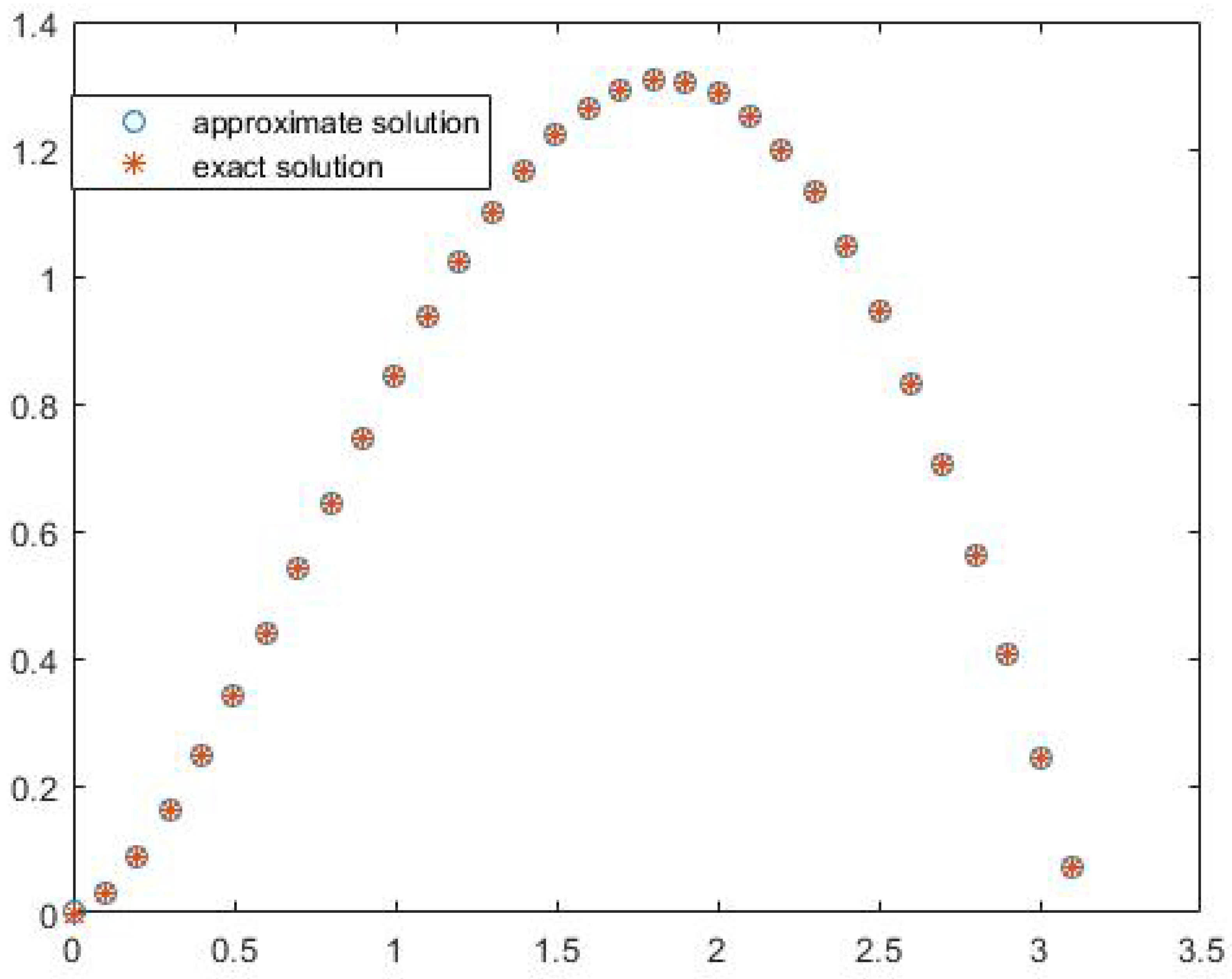
When $0<{\alpha }_1<{\alpha }_2<\cdots <{\alpha }_m<1$ in Equation (4), we have the first order class of FDEs. In this case, the following can be shown: $\mathbf{Q}(z;y,\mathbf{A})=d_{\circ }{\sum }_{k=1}^m{A}_k{z}^{{\alpha }_k}$ and $\mathbf{P}(z;y,\mathbf{A})=\frac{d_{\circ }}{z}\mathbf{Q}(z;y,\mathbf{A})$. So, the approximate solution of Equation (4) consists of two parts: $y_{\circ }\left(t\right)=d_{\circ }$ and $y_N\left(t\right)={\mathcal{L}}_N^{-1}[\frac{\widehat{f}(.)}{\mathbf{Q}(.;y,\mathbf{A})}]\left(t\right)$. For this example, let us consider $d_{\circ }=1$, ${\alpha }_1=\frac{1}{4},{\alpha }_2=\frac{1}{2}$, $A_1=1,A_2=2,\gamma =-1$ and $f\left(t\right)=t^{\frac{1}{4}}+t^{\frac{1}{2}}-7t^{\frac{3}{4}}+t$. The numerical results with $N=1000$ are given in Figure 1 and

Table 1. Exact and approximate values of the proposed method for Example Section 3.1.

t	$\mathbf{Exact}\mathbf{Solution}$	$\mathbf{Approximate}\mathbf{Solution}$	Error
$0.0$	$0.0000$	$0.0005$	$0.0005$
$0.3$	$0.1619$	$0.1625$	$0.0006$
$0.6$	$0.4374$	$0.4376$	$0.0002$
$0.9$	$0.7431$	$0.7432$	$0.0001$
$1.2$	$1.0210$	$1.0213$	$0.0003$
$1.5$	$1.2217$	$1.2224$	$0.0007$
$1.8$	$1.3066$	$1.3067$	$0.0002$
$2.1$	$1.2509$	$1.2510$	$0.0001$
$2.4$	$1.0464$	$1.0472$	$0.0008$
$2.7$	$0.7023$	$0.7029$	$0.0006$
$3.0$	$0.2444$	$0.2447$	$0.0003$

in which the maximum error is given by $8.9433e-04$.

As a second example for this case, let us consider the following equation:

$$\begin{array}{cc}\hfill {}^C{D}_{0^{+}}^{\alpha }y\left(t\right)+y\left(t\right)& =t^4-{\displaystyle \frac{1}{2}}{t}^3-{\displaystyle \frac{3}{\mathsf{\Gamma }(4-\alpha )}}{t}^{3-\alpha }+{\displaystyle \frac{24}{\mathsf{\Gamma }(5-\alpha )}}{t}^{4-\alpha },\hfill \\ \hfill & y\left(0\right)=0,0<\alpha <1,t\in [0,5],\hfill \end{array}$$

(23)

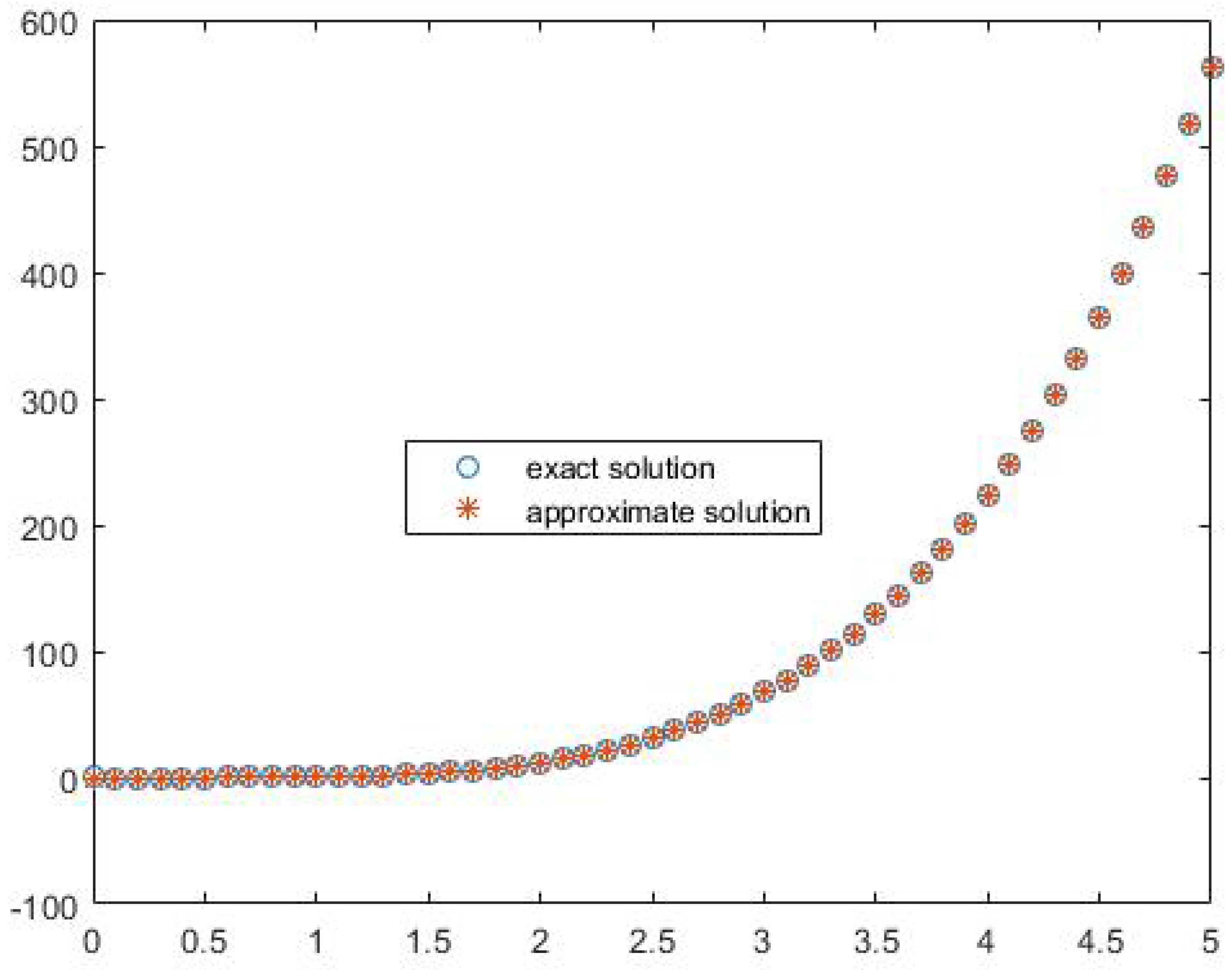
whose the exact solution is given by $y\left(t\right)=t^4-{\displaystyle \frac{1}{2}}{t}^3$ [22]. In

Table 2. Exact and approximate values of the proposed method with $\alpha =0.8$ and $N=1000$ for Equation (23).

t	$\mathbf{Exact}\mathbf{Solution}$	$\mathbf{Approximate}\mathbf{Solution}$
$0.0$	$0.0000$	$0.0000$
$0.5$	$0.0000$	$0.0000$
$1.0$	$0.5000$	$0.5000$
$1.5$	$3.3750$	$3.3750$
$2.0$	$12.0000$	$12.0000$
$2.5$	$31.2500$	$31.2500$
$3.0$	$67.5000$	$67.5000$
$3.5$	$128.6250$	$128.6250$
$4.0$	$224.0000$	$224.0000$
$4.5$	$364.5000$	$364.5000$
$5.0$	$562.5000$	$562.5000$

, we list the exact and approximate solutions for $\alpha =0.8$ and $N=1000$. Maximum absolute errors using this method with different values of $\alpha$ and N are presented in

Table 3. Maximum error of the proposed method with different values of $\alpha$ and N for Equation (23).

	$\mathit{\alpha }=0.8$			$\mathit{\alpha }=0.4$
$\mathit{t}$	$\mathit{N}\mathbf{=}\mathit{1000}$	$\mathit{N}\mathbf{=}\mathit{2000}$	$\mathit{N}\mathbf{=}\mathit{4000}$	$\mathit{N}\mathbf{=}\mathit{1000}$	$\mathit{N}\mathbf{=}\mathit{2000}$	$\mathit{N}\mathbf{=}\mathit{4000}$
$0.0$	$7.5582e-8$	$1.197e-10$	$1.310e-13$	$2.011e-8$	$1.187e-10$	$2.301e-13$
$0.5$	$2.9539e-8$	$1.094e-10$	$1.037e-13$	$2.000e-8$	$1.194e-09$	$2.037e-13$
$1.0$	$3.2312e-8$	$1.006e-10$	$1.124e-13$	$1.908e-8$	$1.105e-09$	$2.325e-13$
$1.5$	$4.6016e-8$	$0.923e-10$	$1.130e-13$	$1.901e-8$	$0.921e-10$	$2.159e-13$
$2.0$	$1.2322e-8$	$0.845e-10$	$1.167e-13$	$1.852e-8$	$0.841e-10$	$2.167e-13$
$2.5$	$5.1819e-8$	$0.772e-10$	$1.248e-13$	$1.798e-8$	$0.767e-10$	$1.769e-13$
$3.0$	$1.5116e-8$	$0.705e-10$	$1.216e-13$	$1.775e-8$	$0.705e-10$	$1.726e-13$
$3.5$	$6.2418e-8$	$0.641e-10$	$1.049e-13$	$1.687e-8$	$0.631e-10$	$1.649e-13$
$4.0$	$3.4868e-8$	$0.581e-10$	$1.140e-13$	$1.625e-8$	$0.538e-10$	$1.591e-13$
$4.5$	$6.5410e-8$	$0.526e-10$	$1.154e-13$	$1.527e-8$	$0.502e-10$	$1.514e-13$
$5.0$	$4.2626e-8$	$0.475e-10$	$1.103e-13$	$1.499e-8$	$0.397e-10$	$1.445e-13$

. From the perspective of error values, our suggested approach is more effective by increasing N. A comparison between the obtained results in [22] and that reported by the proposed scheme reveals that the accuracy of our method is higher than all previously proposed ones since the maximum error given in this reference is of the order $e-06$. The results of the numerical simulations are plotted in Figure 2.

3.2. FDE with Delay Term

If in Equation (22), the non-FDE part for $c>0$ is as follows,

$$\mathbf{J}y\left(t\right)=B\left\{\begin{array}{cc}0,& 0\le t<c,\\ y(t-c),& c\le t,\end{array}\right.$$

it is easy to draw the Laplace transform of it based on the technical method of Section 2 as $B{e}^{-cz}\widehat{y}\left(z\right)$. To test this method for this example with exact solution $y\left(t\right)=t{e}^t$, we take ${\alpha }_1=0.1$, ${\alpha }_2=0.22$, ${\alpha }_3=\sqrt{2}$, ${\alpha }_4=\sqrt{5}$, as well as $A_1=A_3=-1$, $A_2=A_4=3$, $B=1,c=1.5$, $\gamma =0$, $d_{\circ }=d_1=0$ and $d_2=1$.

Table 4. Maximum error of the proposed method with different values of N for Example Section 3.2.

		Error of the Approximate Solution
$\mathit{t}$	$\mathbf{Exact}\mathbf{Solution}$	$\mathit{N}\mathbf{=}\mathit{1000}$	$\mathit{N}\mathbf{=}\mathit{2000}$	$\mathit{N}\mathbf{=}\mathit{4000}$
$0.0$	$0.0000$	$0.0065$	$7.227e-6$	$1.301e-10$
$0.5$	$0.8243$	$0.0007$	$6.894e-6$	$1.247e-10$
$1.0$	$2.7182$	$0.0012$	$5.054e-6$	$1.191e-10$
$1.5$	$6.7225$	$0.0011$	$5.203e-6$	$1.112e-10$
$2.0$	$14.7781$	$0.0052$	$5.111e-6$	$1.097e-10$
$2.5$	$30.4562$	$0.0060$	$5.072e-6$	$1.048e-10$
$3.0$	$60.2566$	$0.0056$	$4.774e-6$	$1.018e-10$
$3.5$	$115.9040$	$0.0065$	$4.002e-6$	$9.049e-11$
$4.0$	$218.3926$	$0.0035$	$3.332e-6$	$8.141e-11$
$4.5$	$405.0770$	$0.0039$	$2.657e-6$	$7.754e-11$
$5.0$	$742.0657$	$0.0022$	$1.011e-6$	$5.914e-11$

compares the numerical results of the exact and the approximate solution obtained by the proposed approach. As can be seen, the best performance is obtained by our approach, which also achieves good approximation results by increasing N. Similarly, the graphs of $y\left(t\right)$ and $y_N\left(t\right)$, for $N=1000$, are shown in Figure 3.

3.3. Second Order FDE

If the initial condition to be substituted with the boundary condition for ${\alpha }_m<2$, then we have the boundary value second order FDE. In this case, it is possible to use the multiple solution as well as the boundary value ordinary differential equations. The practical examination is implemented, giving us the following problem:

$$\begin{array}{cc}\hfill {}^C{D}_{0^{+}}^{1.5}y\left(t\right)-3^C{D}_{0^{+}}^{0.5}y\left(t\right)& + 2y\left(t\right)=f\left(t\right),t\in (0,5),\hfill \\ \hfill y\left(0\right)& =0,\hfill \\ \hfill y^{\prime }\left(0\right)& =\beta ,\hfill \end{array}$$

(24)

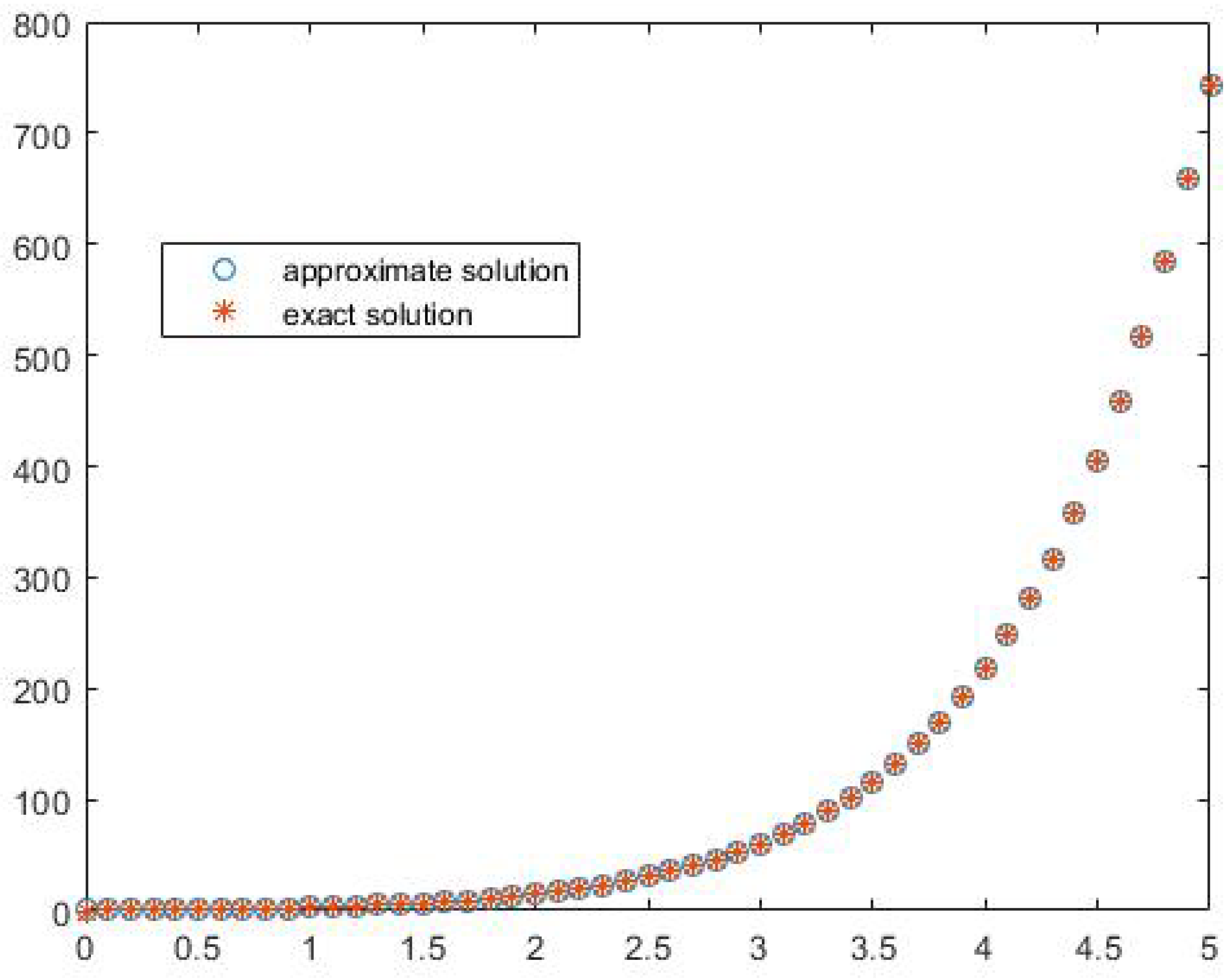
where $f\left(t\right)$ is computed by replacing $y\left(t\right)=t{e}^{-t}$ in Equation (24). Now, a roots-finder method, such as the iterative Picard method [23], bisection method [24] and so on, can be used to determinate the parameter $\beta$. The numerical results for the exact and approximate solutions for $\beta =0$ and $N=1000$ are given in Figure 4 and

Table 5. Exact and approximate values of the proposed method for Equation (24).

t	$\mathbf{Exact}\mathbf{Solution}$	$\mathbf{Approximate}\mathbf{Solution}$	$\mathbf{Error}$
$0.0$	$0.0000$	$0.0065$	$0.0065$
$0.5$	$0.8243$	$0.8251$	$0.0007$
$1.0$	$2.7182$	$2.7195$	$0.0012$
$1.5$	$6.7225$	$6.7236$	$0.0011$
$2.0$	$14.7781$	$14.7833$	$0.0052$
$2.5$	$30.4562$	$30.4622$	$0.0060$
$3.0$	$60.2566$	$60.2622$	$0.0056$
$3.5$	$115.9040$	$115.9106$	$0.0065$
$4.0$	$218.3926$	$218.3961$	$0.0035$
$4.5$	$405.0770$	$405.0810$	$0.0039$
$5.0$	$742.0657$	$742.0680$	$0.0022$

.

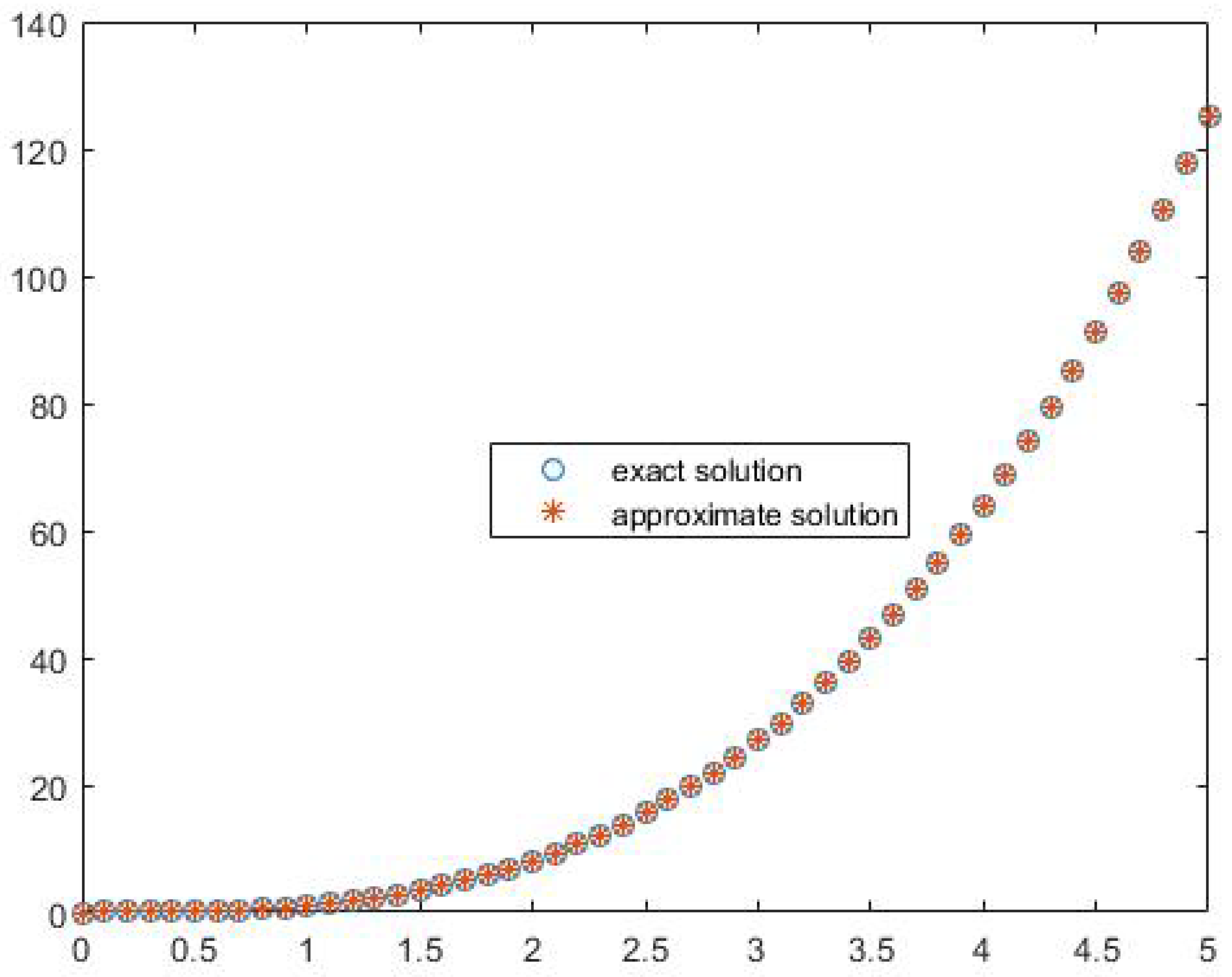
As a second example for this case, let us consider the following equation [25]:

$$\begin{array}{cc}\hfill {}^C{D}_{0^{+}}^{2}y\left(t\right)+ {}^C{D}_{0^{+}}^{\alpha }y\left(t\right)& + y\left(t\right)=t^3+6t+{\displaystyle \frac{8.533}{\mathsf{\Gamma }\left(0.25\right)}}{t}^{2.25},t\in [0,1],\hfill \\ \hfill y\left(0\right)& =y^{\prime }\left(0\right)=0.\hfill \end{array}$$

(25)

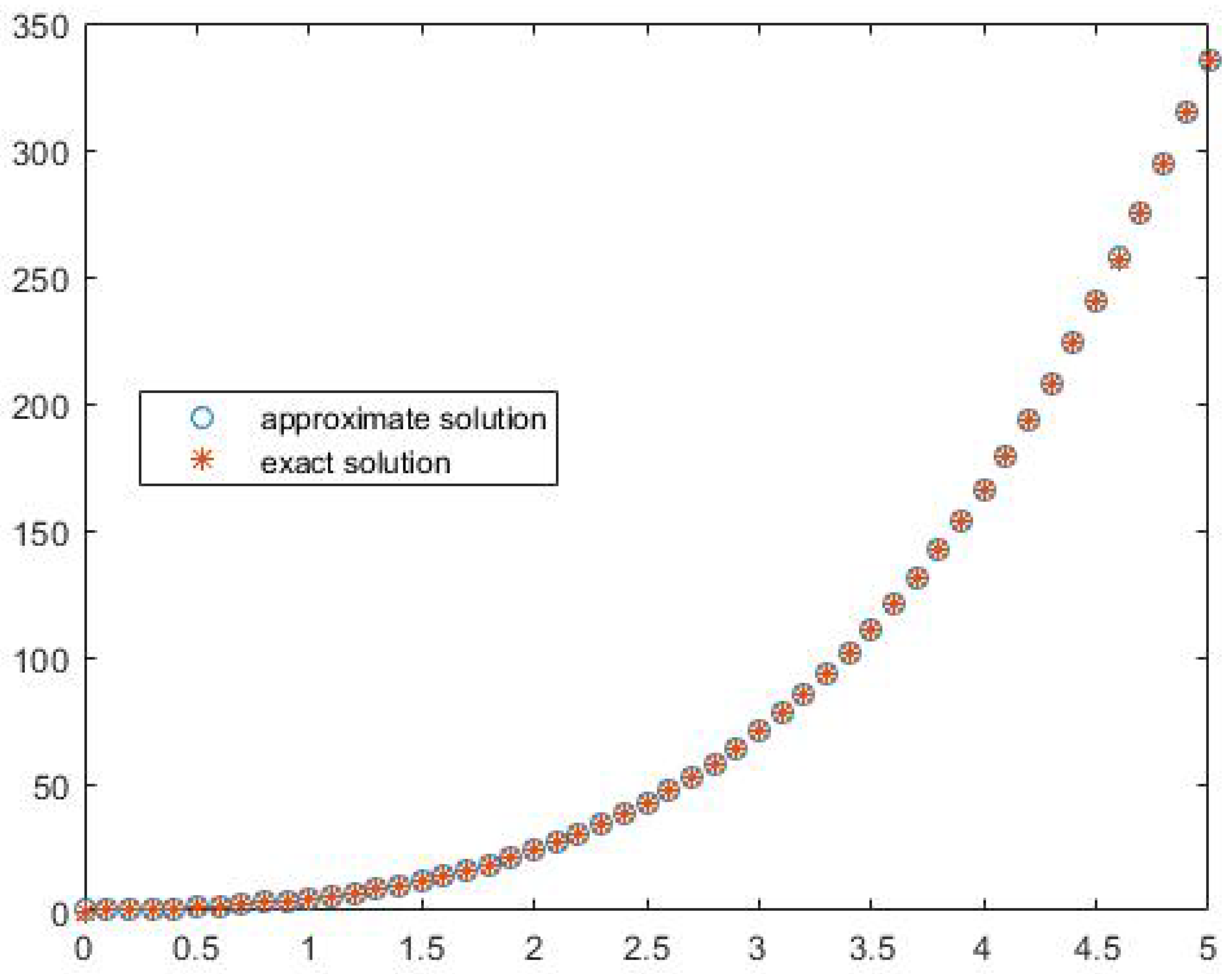
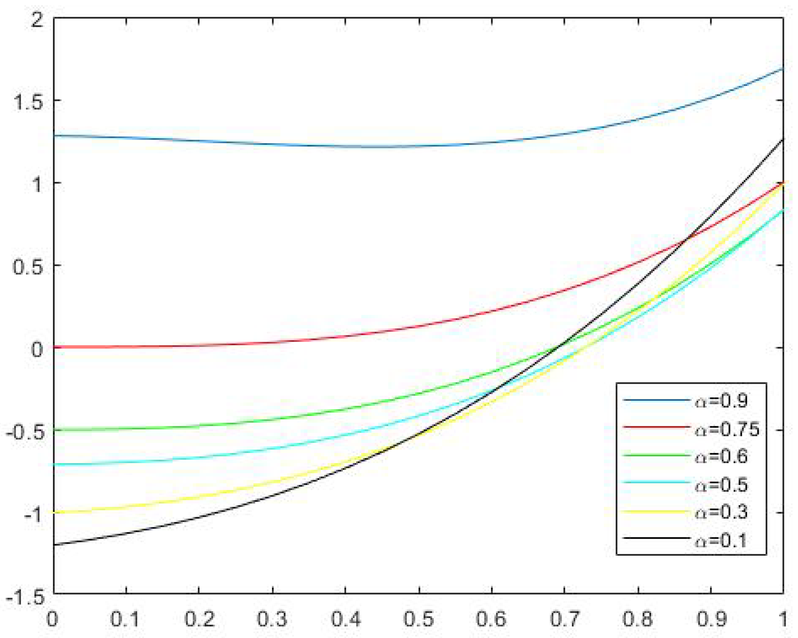
In this case, $y\left(t\right)=t^3$ is the exact solution by selecting $\alpha =\frac{3}{4}$. By applying our method, the maximum absolute error for this equation is obtained as $2.3562e-23$, while the best result that is achieved by using the previous methods is $5.6722e-19$ [26]. The graphs of exact and approximate solution for $N=1000$ are shown in Figure 5. More precisely, we solve this problem for different choices of $\alpha$ as shown in Figure 6. These figures corroborate the validity and efficacy of our method.

4. Conclusions

In this paper, the problem including FDE is solved, based on the Laplace transform method. After taking the Laplace transform, we apply an inverse Laplace transformation. Since the computing of this inverse problem is difficult, we need to apply an efficient numerical scheme. Here, a powerful quadrature rule is used to approximate the integration that appears in the inverse Laplace transform. The convergent rate of our method is similar to the order of the quadrature rule. Additionally, the easy implementation is another advantage of this method (see Equation (16)). Furthermore, it is shown that this method has an exponential convergence for $t>\frac{N}{lnN}$. Hence, the results are very sensitive to the choice of N. Some various kinds of FDEs are brought into this work. We can survey the other typical problems with either the finite interval domains or even by having the periodical solution. One can apply this scheme for them in future.

References

- Ren, H.P.; Wang, X.; Fan, J.T.; Kaynak, O. Fractional order sliding mode control of a pneumatic position servo system. J. Frankl. Inst. 2019, 356, 6160–6174. [Google Scholar] [CrossRef]
- Zhang, J.; Jin, Z.; Zhao, Y.; Tang, Y.; Liu, F.; Lu, Y.; Liu, P. Design and implementation of novel fractional-order controllers for stabilized platforms. IEEE Access 2020, 8, 93133–93144. [Google Scholar] [CrossRef]
- Vashisht, R.K.; Peng, Q. Efficient active chatter mitigation for boring operation by electromagnetic actuator using optimal fractional order PDλ controller. J. Mater. Process. Technol. 2020, 276, 116423. [Google Scholar] [CrossRef]
- Sidhardh, S.; Patnaik, S.; Semperlotti, F. Geometrically nonlinear response of a fractional-order nonlocal model of elasticity. Int. J. Non-Linear Mech. 2020, 125, 103529. [Google Scholar] [CrossRef]
- Sánchez-López, C. An experimental synthesis methodology of fractional-order chaotic attractors. Nonlinear Dyn. 2020, 100, 3907–3923. [Google Scholar] [CrossRef]
- Khan, A.; Nigar, U. Sliding mode disturbance observer control based on adaptive hybrid projective compound combination synchronization in fractional-order chaotic systems. J. Control Autom. Electr. Syst. 2020, 31, 885–899. [Google Scholar] [CrossRef]
- Mahto, T.; Malik, H.; Mukherjee, V.; Alotaibi, M.A.; Almutairi, A. Renewable generation based hybrid power system control using fractional order-fuzzy controller. Energy Rep. 2021, 7, 641–653. [Google Scholar]
- Lv, X.; Sun, Y.; Hu, W.; Dinavahi, V. Robust load frequency control for networked power system with renewable energy via fractional-order global sliding mode control. IET Renew. Power Gener. 2021, 15, 1046–1057. [Google Scholar] [CrossRef]
- Farman, M.; Akgül, A.; Ahmad, A.; Imtiaz, S. Analysis and dynamical behavior of fractional-order cancer model with vaccine strategy. Math. Methods Appl. Sci. 2020, 43, 4871–4882. [Google Scholar] [CrossRef]
- Owusu-Mensah, I.; Akinyemi, L.; Oduro, B.; Iyiola, O.S. A fractional order approach to modeling and simulations of the novel COVID-19. Adv. Differ. Equ. 2020, 2020, 1–21. [Google Scholar]
- Zeid, S.S. Approximation methods for solving fractional equations. Chaos Solitons Fractals 2019, 125, 171–193. [Google Scholar] [CrossRef]
- Lloyd, N.G. Remarks on generalising Rouché’s theorem. J. Lond. Math. Soc. 1979, 2, 259–272. [Google Scholar] [CrossRef]
- Kilbas, A.A.; Srivastava, H.M.; Trujillo, J.J. Theory and Applications of Fractional Differential Equations; Elsevier: Amsterdam, The Netherlands, 2006. [Google Scholar]
- Wiora, J.; Wiora, A. Influence of methods approximating fractional-order differentiation on the output signal illustrated by three variants of Oustaloup filter. Symmetry 2020, 12, 1898. [Google Scholar] [CrossRef]
- Kapoulea, S.; Psychalinos, C.; Elwakil, A.S. Minimization of spread of time-constants and scaling factors in fractional-order differentiator and integrator realizations. Circuits Syst. Signal Process. 2018, 37, 5647–5663. [Google Scholar] [CrossRef]
- Jia, Z.; Liu, C. Fractional-order modeling and simulation of magnetic coupled boost converter in continuous conduction mode. Int. J. Bifurc. Chaos 2018, 28, 1850061. [Google Scholar] [CrossRef]
- Kartci, A.; Agambayev, A.; Farhat, M.; Herencsar, N.; Brancik, L.; Bagci, H.; Salama, K.N. Synthesis and optimization of fractional-order elements using a genetic algorithm. IEEE Access 2019, 7, 80233–80246. [Google Scholar] [CrossRef]
- Sheen, D.; Sloan, I.H.; Thomée, V. A parallel method for time discretization of parabolic equations based on Laplace transformation and quadrature. IMA J. Numer. Anal. 2003, 23, 269–299. [Google Scholar] [CrossRef] [Green Version]
- Uddin, M.; Taufiq, M. On the approximation of Volterra integral equations with highly oscillatory Bessel kernels via Laplace transform and quadrature. Alex. Eng. J. 2018, 58, 413–417. [Google Scholar] [CrossRef]
- Uddin, M.; Khan, S. On the numerical solution of fractional order differential equations using transforms and quadrature. TWMS J. Appl. Eng. Math. 2019, 8, 267–274. [Google Scholar]
- McLean, W.; Thomée, V. Maximum-norm error analysis of a numerical solution via Laplace transformation and quadrature of a fractional-order evolution equation. IMA J. Numer. Anal. 2010, 30, 208–230. [Google Scholar] [CrossRef]
- Bhrawy, A.H.; Baleanu, D.; Assas, L.M. Efficient generalized Laguerre-spectral methods for solving multi-term fractional differential equations on the half line. J. Vib. Control 2014, 20, 973–985. [Google Scholar] [CrossRef]
- Carothers, D.; Ingham, W.; Liu, J.; Lyons, C.; Marafino, J.; Parker, G.E.; Wilk, D. An Overview of the Modified Picard Method; Department of Mathematics and Statistics, Physics, James Madison University: Harrisonburg, VA, USA, 2004. [Google Scholar]
- Solanki, C.; Thapliyal, P.; Tomar, K. Role of bisection method. Int. J. Comput. Appl. Technol. Res. 2014, 3, 535. [Google Scholar] [CrossRef]
- Ford, N.J.; Connolly, J.A. Systems-based decomposition schemes for the approximate solution of multi-term fractional differential equations. J. Comput. Appl. Math. 2009, 229, 382–391. [Google Scholar] [CrossRef] [Green Version]
- Ahmad, S. On the Numerical Solution of Linear Multi-Term Fractional Order Differential Equations Using Laplace Transform and Quadrature. PJCIS 2017, 2, 43–49. [Google Scholar]
Figure 1.
Comparing the exact and the approximate solutions with for Example Section 3.1.
Figure 2.
Comparing the exact and the approximate solutions with and for Equation (23).
Figure 3.
Comparing the exact and the approximate solutions for Example Section 3.2.
Figure 4.
Comparing the exact and the approximate solutions for Equation (24).
Figure 5.
Comparing the exact and the approximate solutions for Equation (25).
Figure 6.
Approximate solutions of Equation (25) for different values of .