

Enhancement in Thermal Energy and Solute Particles Using Hybrid Nanoparticles by Engaging Activation Energy and Chemical Reaction over a Parabolic Surface via Finite Element Approach


Abstract
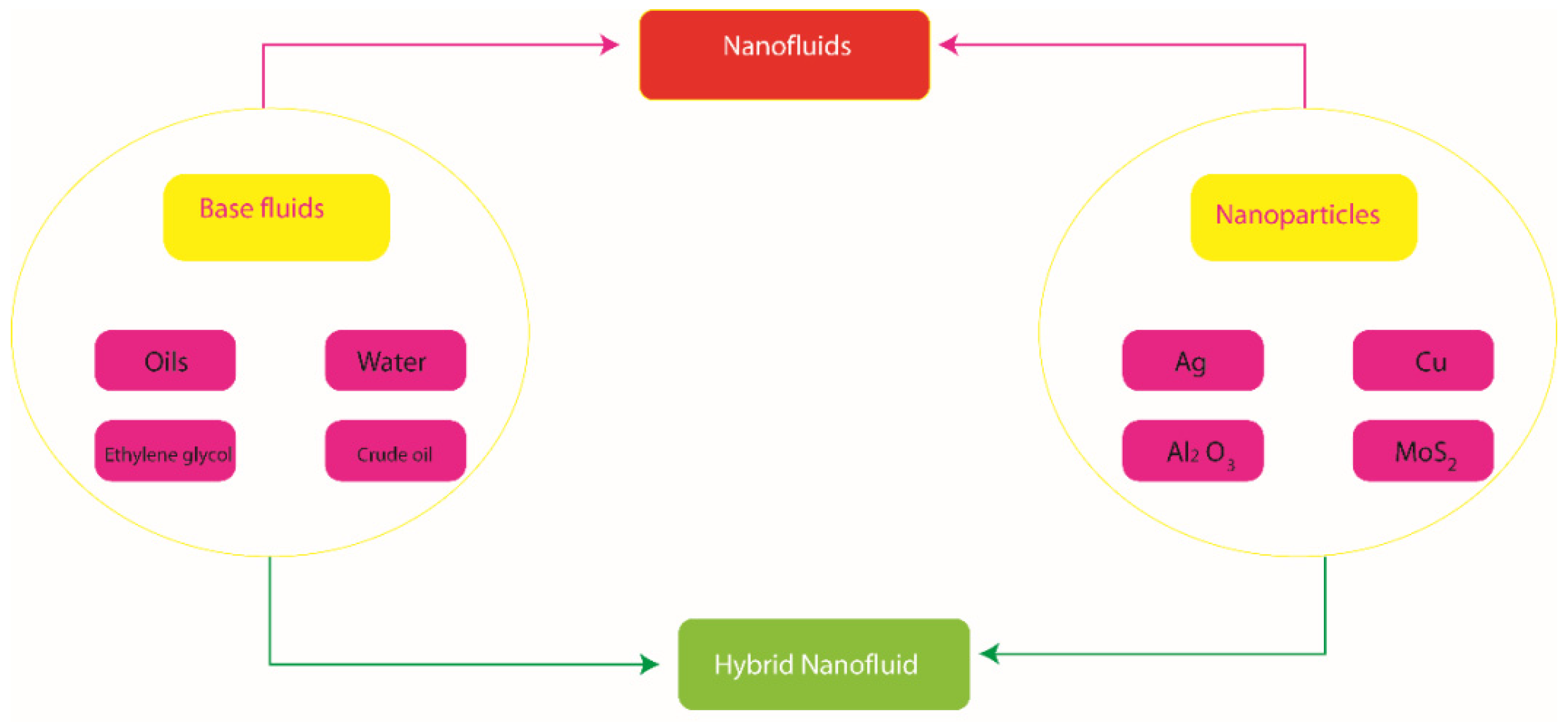
:1. Introduction
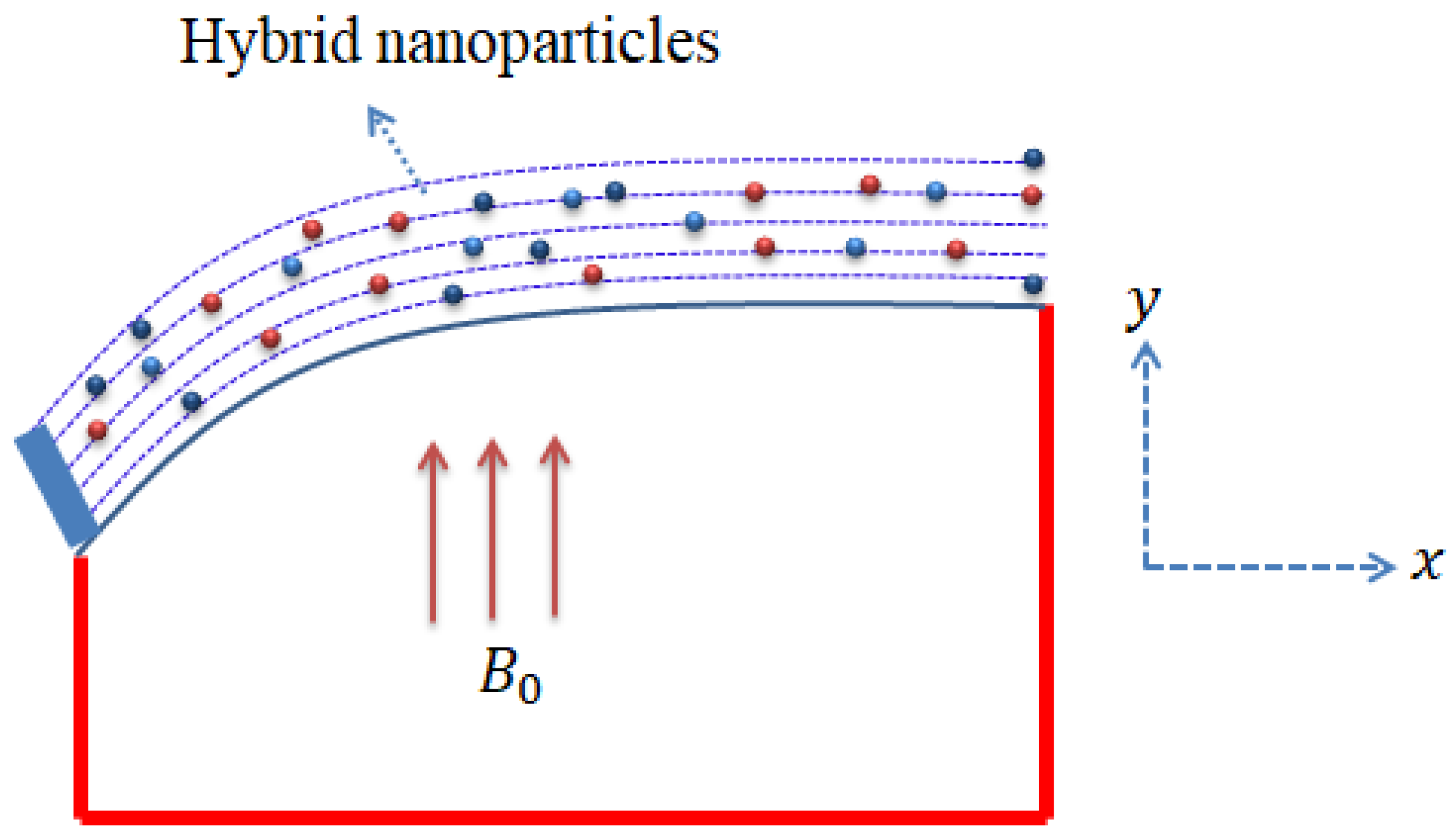
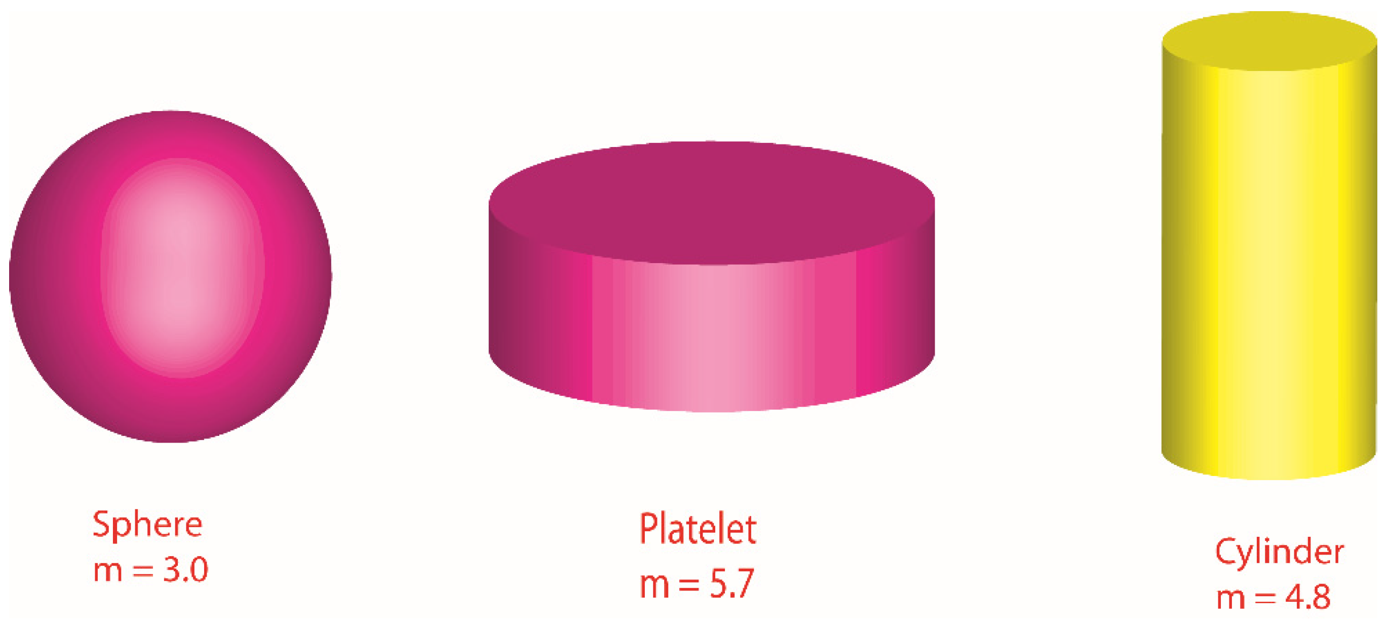
2. Formulation of Physical Model
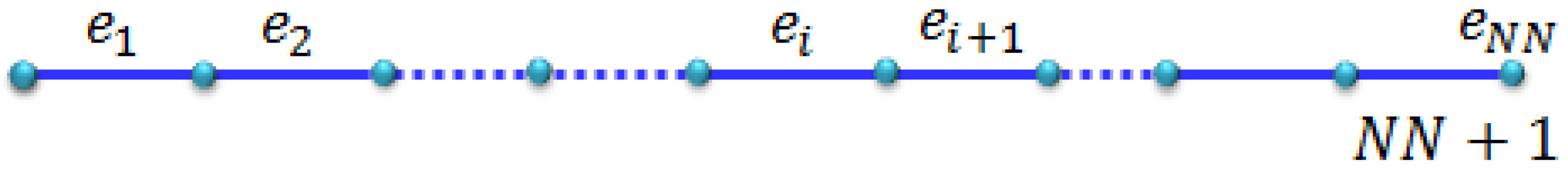
3. Grid Independent Analysis and Numerical Approach
4. Results and Discussion
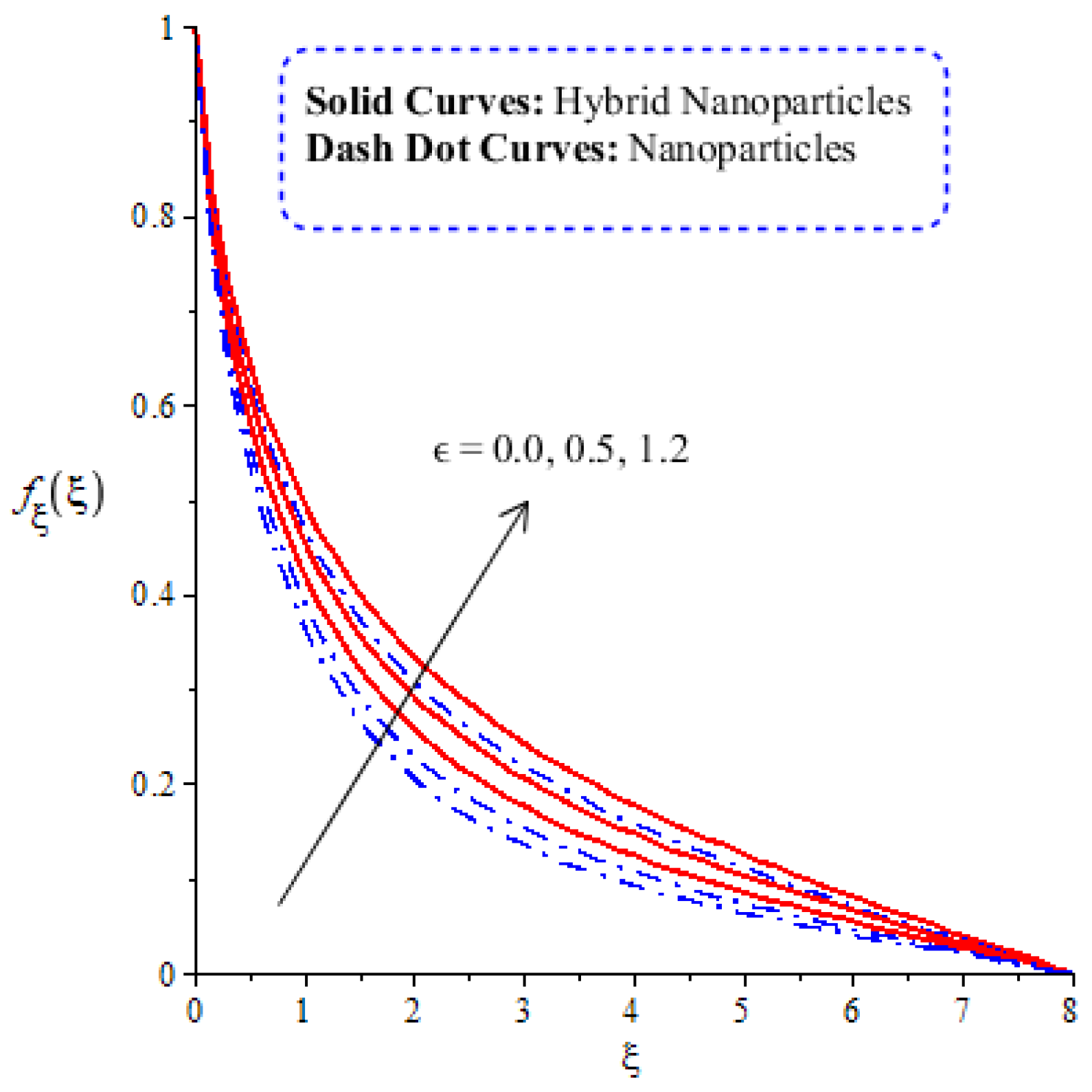
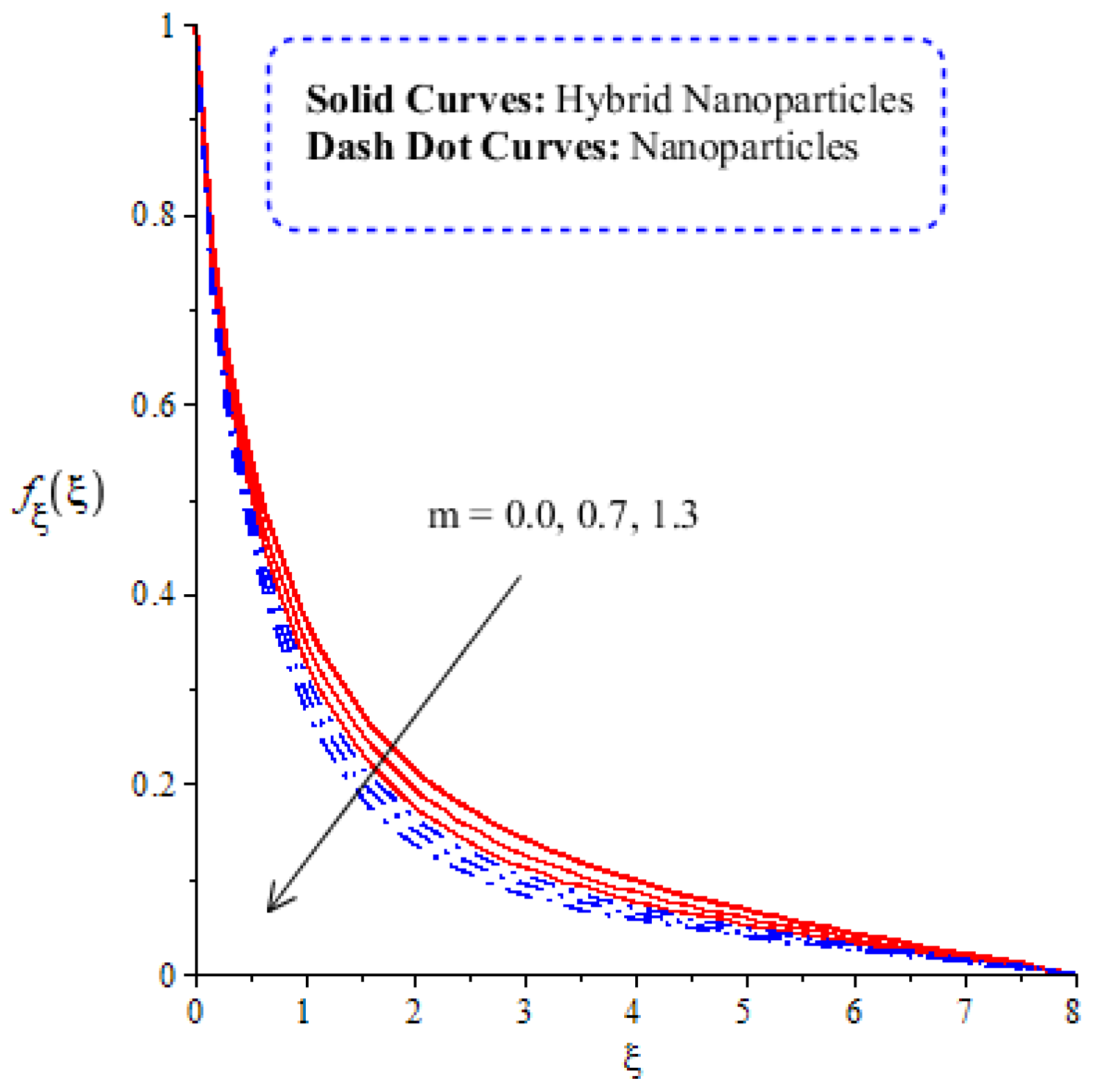
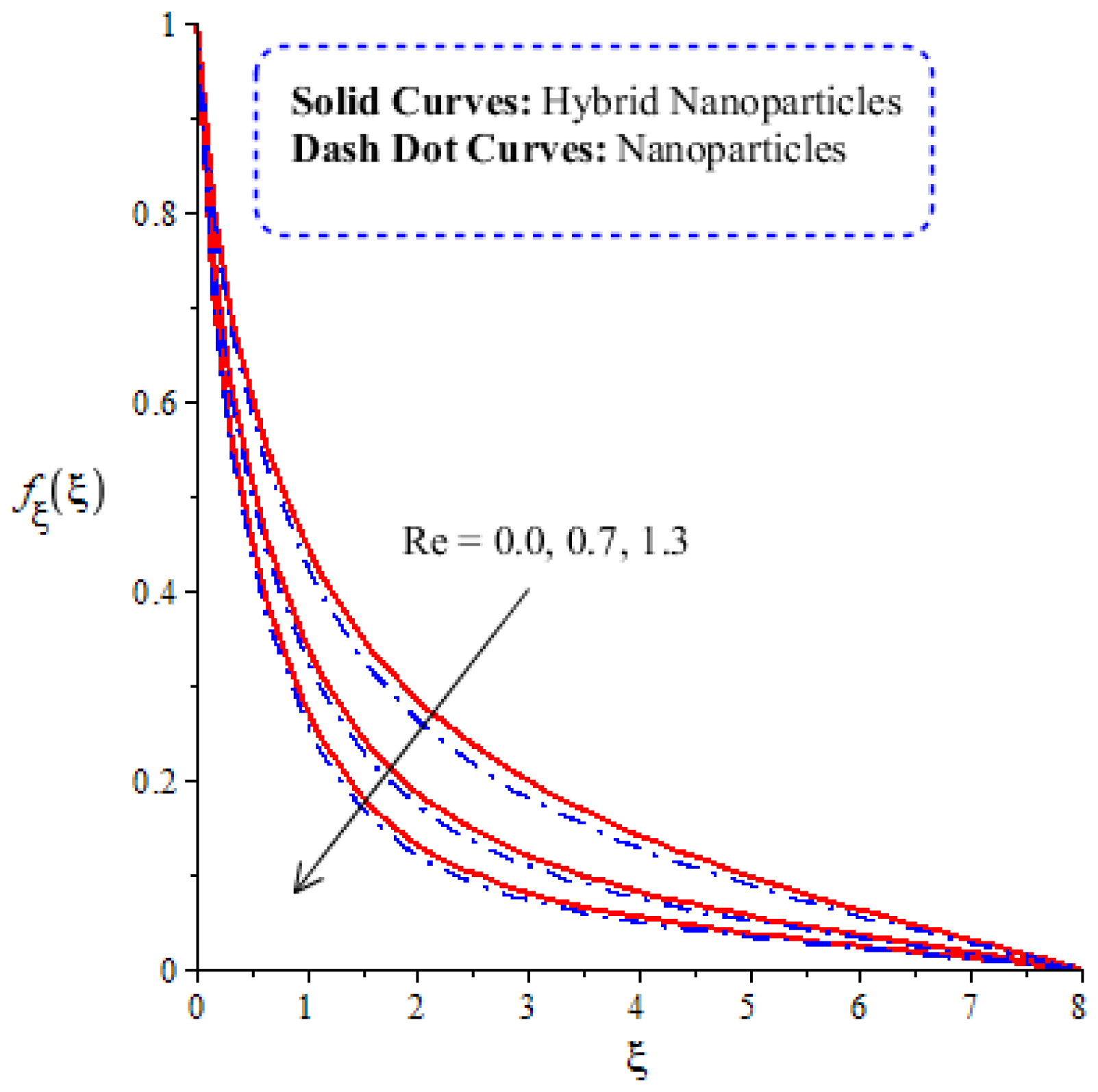
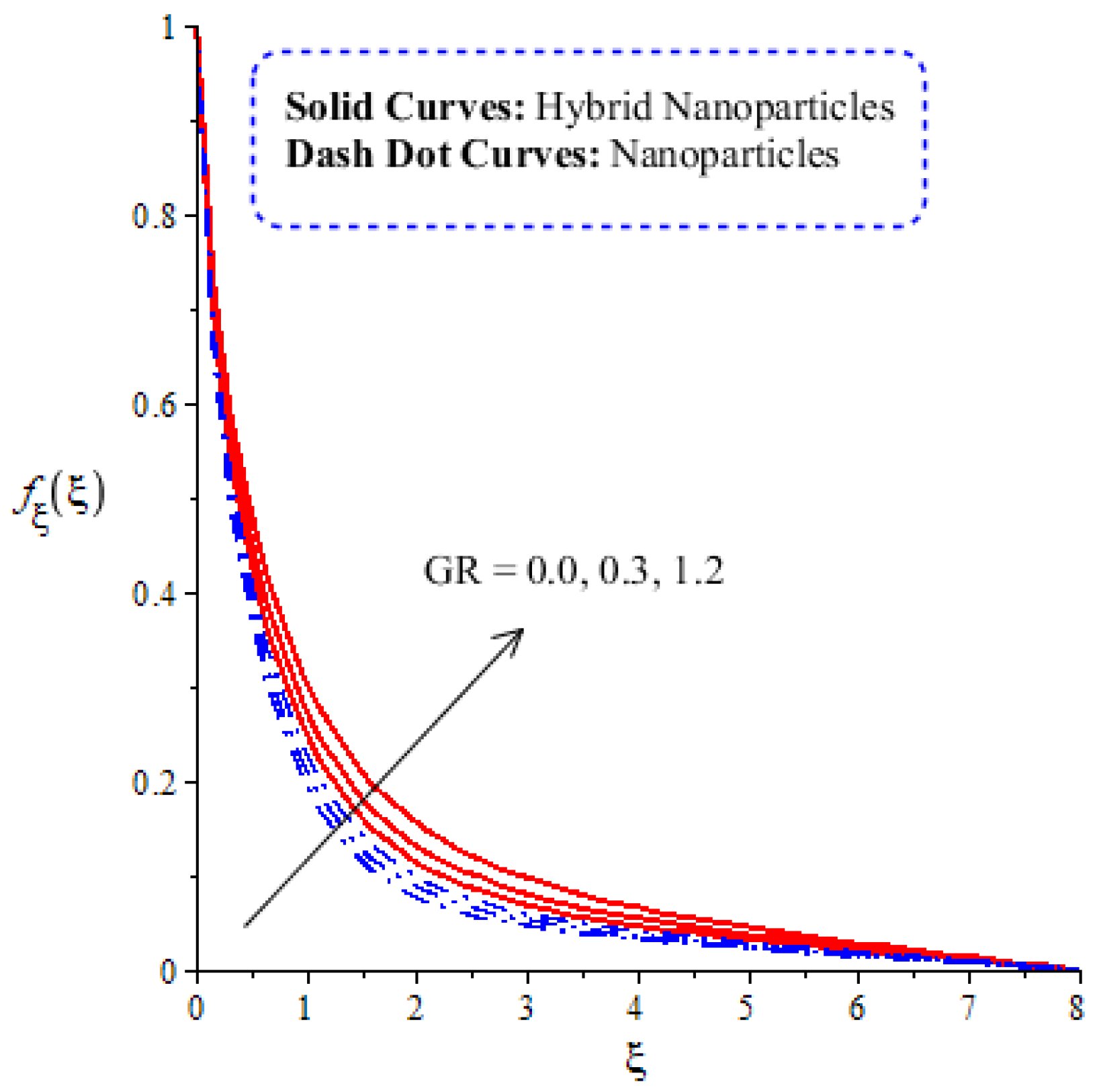
4.1. Comparative Analysis of Flow Behavior in Hybrid Nanoparticles and Nanoparticles
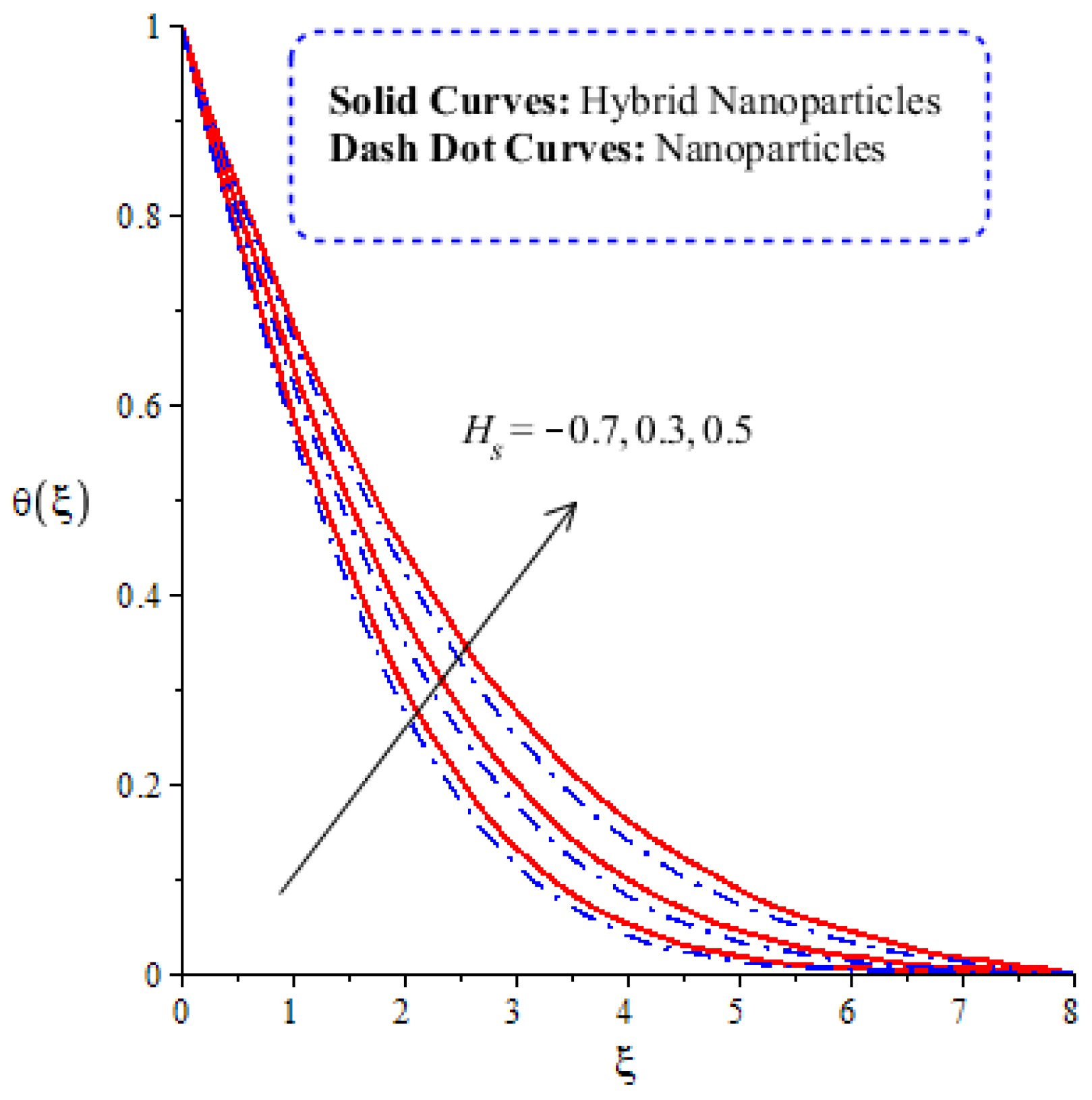
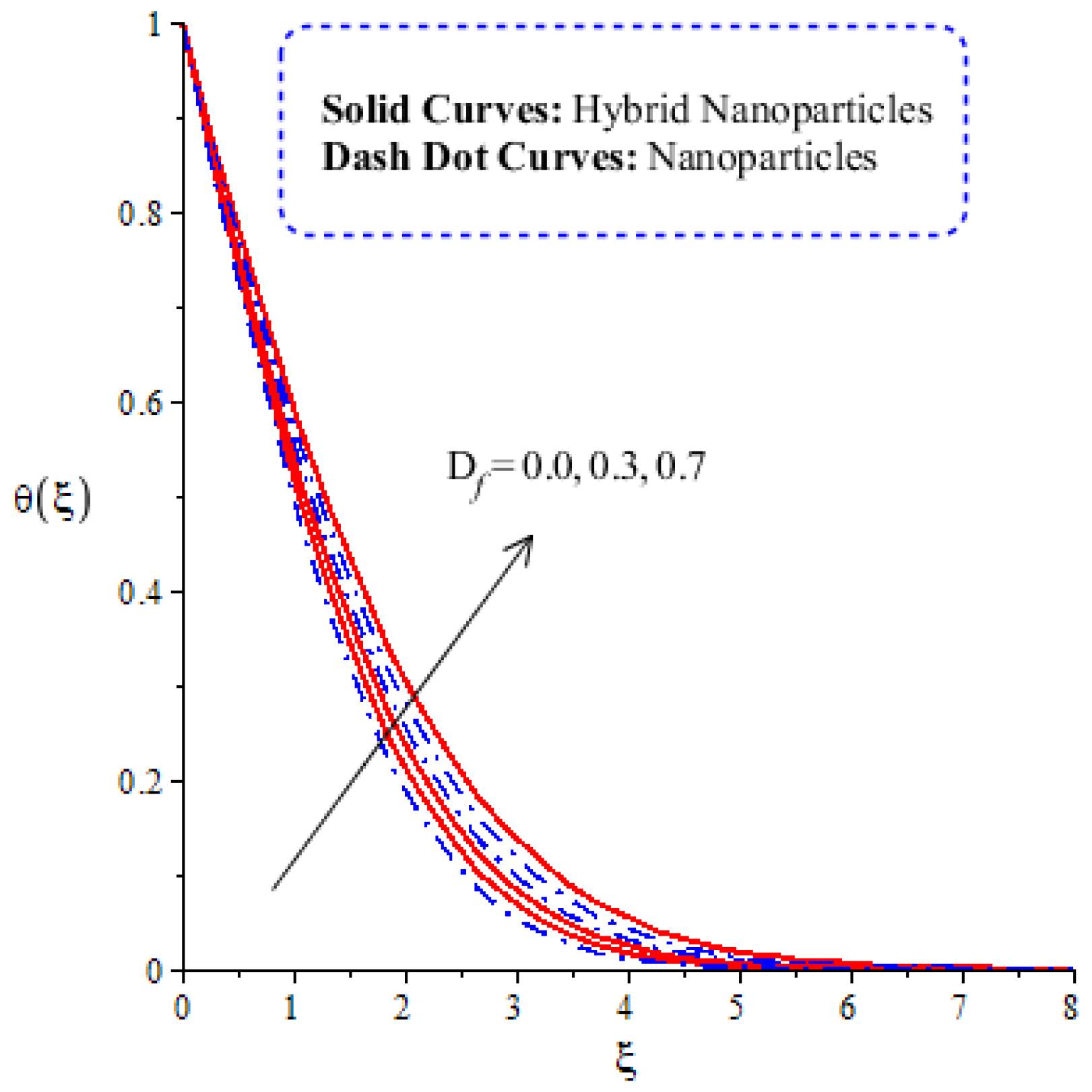
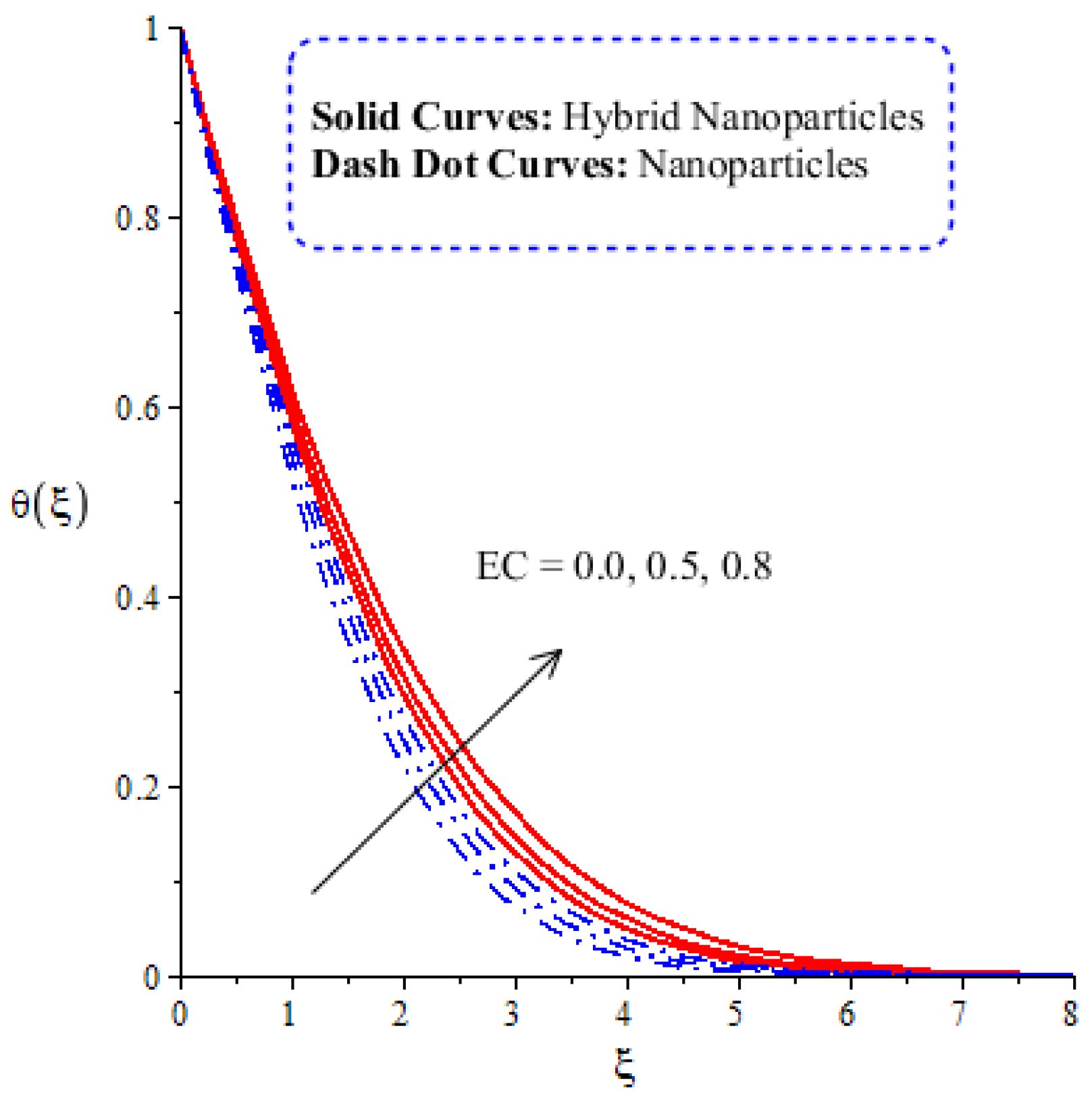
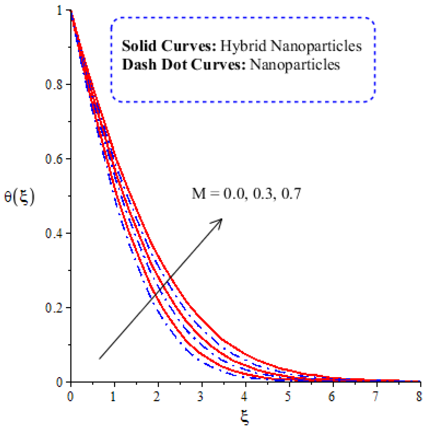
4.2. Comparative Analysis of Thermal Energy in Hybrid Nanoparticles and Nanoparticles
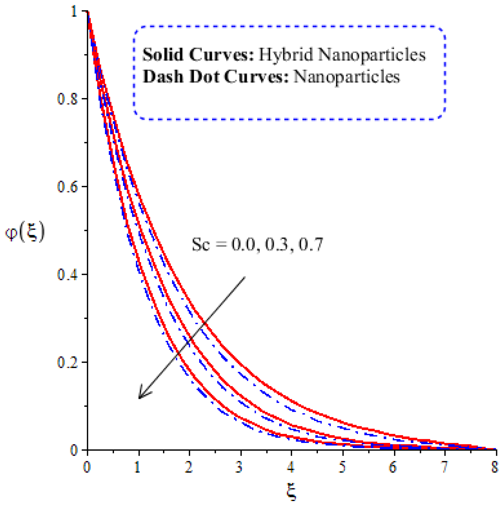
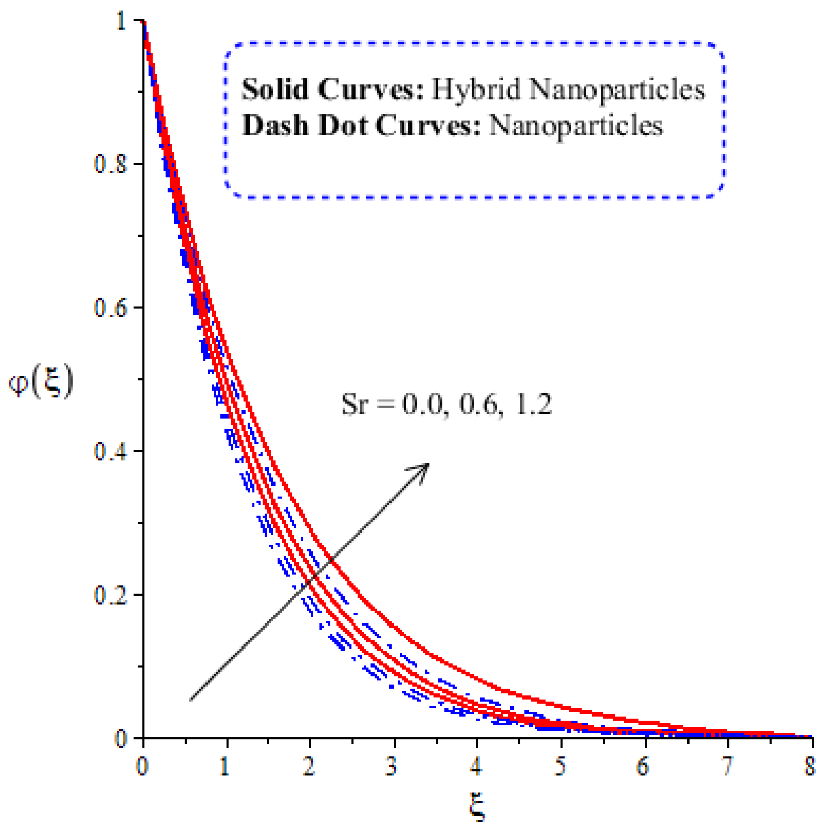
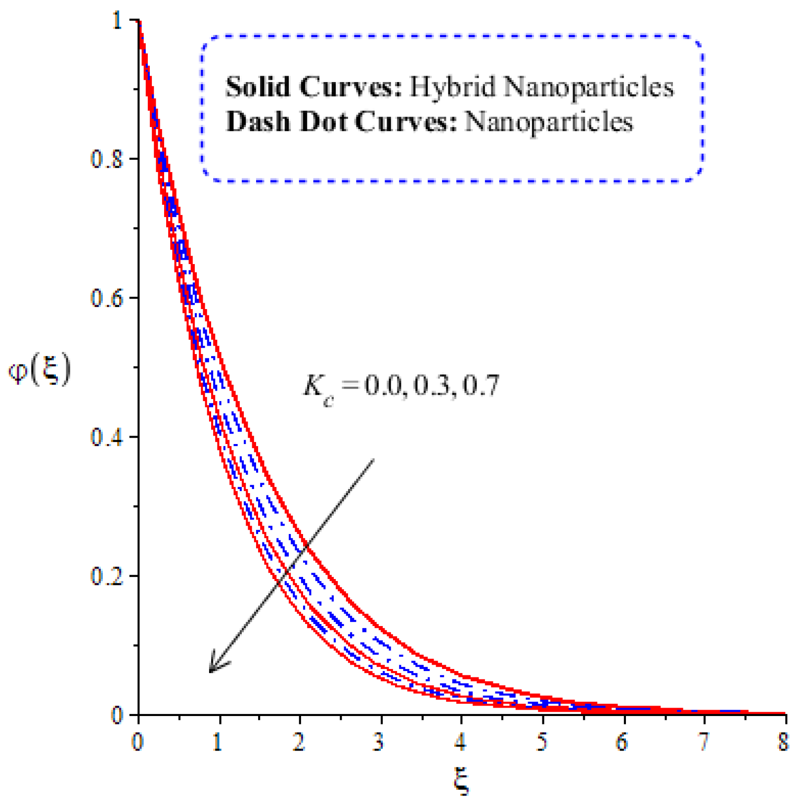
4.3. Comparative Analysis of Solute Particles in Hybrid Nanoparticles and Nanoparticles
4.4. Comparative Simulations of Gradient Temperature, Surface Force and Rate of Solute Particles in Hybrid Nanoparticles and Nanoparticles
5. Prime Consequences of Current Model
Author Contributions
Funding
Institutional Review Board Statement
Informed Consent Statement
Data Availability Statement
Conflicts of Interest
Nomenclature
| Symbols | Used for | Symbols | Used for |
| Velocity components (m/s) | Space coordinates | ||
| Gravitational force (N) | Weight functions | ||
| Power law index number | Temperature and ambient temperature | ||
| Concentration and ambient concentration (Kgm−3) | Magnetic induction | ||
| Thermal conductivity (Wm−1) | Thermal diffusion | ||
| Mass diffusion (m2s−1) | Concentration susceptibility | ||
| Specific heat capacitance (JKg−1K) | Heat generation | ||
| Chemical reaction (s−1) | Fluid mean temperature | ||
| Activation energy (JKg−1K) | |||
| Constants | Dimensionless velocity | ||
| Thermal Grashof | Bio-convection Rayleigh | ||
| Magnetic field | Prandtl number | ||
| Eckert number | Heat generation number | ||
| Hybrid nanofluid | Dufour number | ||
| Schmidt number | Soret number | ||
| Chemical reaction number | Nusselt number | ||
| Sherwood number | Reynolds number | ||
| Size number of nanoparticles | Skin friction coefficient | ||
| Copper and aluminum oxide | Ethylene glycol | ||
| Greek Symbols | |||
| Electrically conductivity (S.m−1) | Volumetric coefficients | ||
| Fluid density (Kg.m−3) | Infinite number | ||
| Stream function | Dimensionless temperature | ||
| Dimensionless concentration | Volume fractions | ||
| Independent variable | Fluid number | ||
| Shear stress (N.m−2) | Euler number | ||
| Temeprature differnece (K) | Fluid number | ||
References
- Islam, S.; Shah, A.; Zhou, C.Y.; Ali, I. Homotopy perturbation analysis of slider bearing with Powell–Eyring fluid. Z. Für Angew. Math. Und Phys. 2009, 60, 1178–1193. [Google Scholar] [CrossRef]
- Patel, M.; Timol, M.G. Numerical treatment of Powell–Eyring fluid flow using method of satisfaction of asymptotic boundary conditions (MSABC). Appl. Numer. Math. 2009, 59, 2584–2592. [Google Scholar] [CrossRef]
- Khan, N.A.; Aziz, S.; Khan, N.A. MHD flow of Powell–Eyring fluid over a rotating disk. J. Taiwan Inst. Chem. Eng. 2014, 45, 2859–2867. [Google Scholar] [CrossRef]
- Hayat, T.; Makhdoom, S.; Awais, M.; Saleem, S.; Rashidi, M.M. Axisymmetric Powell-Eyring fluid flow with convective boundary condition: Optimal analysis. Appl. Math. Mech. 2016, 37, 919–928. [Google Scholar] [CrossRef]
- Krishna, P.M.; Sandeep, N.; Reddy, J.R.; Sugunamma, V. Dual solutions for unsteady flow of Powell-Eyring fluid past an inclined stretching sheet. J. Nav. Archit. Mar. Eng. 2016, 13, 89–99. [Google Scholar] [CrossRef] [Green Version]
- Kumar, D.; Ramesh, K.; Chandok, S. Mathematical modeling and simulation for the flow of magneto-Powell-Eyring fluid in an annulus with concentric rotating cylinders. Chin. J. Phys. 2020, 65, 187–197. [Google Scholar] [CrossRef]
- Abdelsalam, S.I.; Sohail, M. Numerical approach of variable thermophysical features of dissipated viscous nanofluid comprising gyrotactic micro-organisms. Pramana J. Phys. 2020, 94, 1–12. [Google Scholar] [CrossRef]
- Sohail, M.; Naz, R. Modified heat and mass transmission models in the magnetohydrodynamic flow of Sutterby nanofluid in stretching cylinder. Phys. A Stat. Mech. Appl. 2020, 549, 124088. [Google Scholar] [CrossRef]
- Qi, W.H.; Wang, M.P.; Liu, Q.H. Shape factor of nonspherical nanoparticles. J. Mater. Sci. 2005, 40, 2737–2739. [Google Scholar] [CrossRef]
- Maraj, E.N.; Iqbal, Z.; Azhar, E.; Mehmood, Z. A comprehensive shape factor analysis using transportation of MoS2-SiO2/H2O inside an isothermal semi vertical inverted cone with porous boundary. Results Phys. 2018, 8, 633–641. [Google Scholar] [CrossRef]
- Iqbal, Z.; Maraj, E.N.; Azhar, E.; Mehmood, Z. A novel development of hybrid (MoS2−SiO2/H2O) nanofluidic curvilinear transport and consequences for effectiveness of shape factors. J. Taiwan Inst. Chem. Eng. 2017, 81, 150–158. [Google Scholar] [CrossRef]
- Khanafer, K.; Vafai, K. A critical synthesis of thermophysical characteristics of nanofluids. Int. J. Heat Mass Transf. 2011, 54, 4410–4428. [Google Scholar] [CrossRef]
- Saba, F.; Ahmed, N.; Hussain, S.; Khan, U.; Mohyud-Din, S.T.; Darus, M. Thermal analysis of nanofluid flow over a curved stretching surface suspended by carbon nanotubes with internal heat generation. Appl. Sci. 2018, 8, 395. [Google Scholar] [CrossRef] [Green Version]
- Qasim, M.; Khan, Z.H.; Lopez, R.J.; Khan, W.A. Heat and mass transfer in nanofluid thin film over an unsteady stretching sheet using Buongiorno’s model. Eur. Phys. J. Plus 2016, 131, 1–11. [Google Scholar] [CrossRef]
- Awais, M.; Hayat, T.; Ali, A.; Irum, S. Velocity, thermal and concentration slip effects on a magneto-hydrodynamic nanofluid flow. Alex. Eng. J. 2016, 55, 2107–2114. [Google Scholar] [CrossRef] [Green Version]
- Alharbi, S.O.; Nawaz, M.; Nazir, U. Thermal analysis for hybrid nanofluid past a cylinder exposed to magnetic field. AIP Adv. 2019, 9, 115022. [Google Scholar] [CrossRef]
- Mourad, A.; Aissa, A.; Mebarek-Oudina, F.; Jamshed, W.; Ahmed, W.; Ali, H.M.; Rashad, A.M. Galerkin finite element analysis of thermal aspects of Fe3O4-MWCNT/water hybrid nanofluid filled in wavy enclosure with uniform magnetic field effect. Int. Commun. Heat Mass Transf. 2021, 126, 105461. [Google Scholar] [CrossRef]
- Nazir, U.; Nawaz, M.; Alqarni, M.M.; Saleem, S. Finite element study of flow of partially ionized fluid containing nanoparticles. Arab. J. Sci. Eng. 2019, 44, 10257–10268. [Google Scholar] [CrossRef]
- Rasool, G.; Wakif, A. Numerical spectral examination of EMHD mixed convective flow of second-grade nanofluid towards a vertical Riga plate using an advanced version of the revised Buongiorno’s nanofluid model. J. Therm. Anal. Calorim. 2021, 143, 2379–2393. [Google Scholar] [CrossRef]


| Number of Elements | |||
|---|---|---|---|
| 30 | 0.02563511179 | 0.5010430026 | 0.000002753767268 |
| 60 | 0.005590099064 | 0.4622252540 | 0.02471348366 |
| 90 | 0.005472897618 | 0.4564407494 | 0.02293467057 |
| 120 | 0.005415678507 | 0.4535558400 | 0.02208161164 |
| 150 | 0.005381789627 | 0.4518259302 | 0.02158116249 |
| 180 | 0.005359391320 | 0.4506744132 | 0.02125219796 |
| 210 | 0.005343470646 | 0.4498514616 | 0.02101947689 |
| 240 | 0.005331585746 | 0.4492371723 | 0.02084607618 |
| 270 | 0.005322299522 | 0.4487571006 | 0.02071193875 |
| 300 | 0.005314946586 | 0.4483716081 | 0.02060532127 |
| Nanoparticles () | Hybrid Nanoparticles () | ||||||
|---|---|---|---|---|---|---|---|
| Surface Force | Nusselt Number | Sherwood Number | Surface Force | Nusselt Number | Sherwood Number | ||
| 0.2 | 1.924813 | 1.565118 | 0.1384307 | 2.945961 | 2.565701 | 2.1399317 | |
| 0.5 | 0.221389 | 1.754730 | 0.5383389 | 2.549771 | 2.755495 | 2.3398409 | |
| 0.7 | 0.161556 | 1.940713 | 0.8382172 | 2.451139 | 2.946134 | 2.7397592 | |
| 0.0 | 1.512261 | 0.7328196 | 0.1368876 | 2.998115 | 2.533346 | 2.1396489 | |
| 0.5 | 1.946357 | 1.530040 | 0.1381261 | 2.972760 | 2.731219 | 2.3396312 | |
| 0.8 | 1.988206 | 1.725651 | 0.1390913 | 2.982020 | 2.926860 | 2.7395964 | |
| −1.3 | 1.414523 | 1.459182 | 0.1383186 | 2.063254 | 2.460611 | 2.1398258 | |
| 0.3 | 1.262850 | 1.235944 | 0.1269818 | 2.074621 | 2.481310 | 2.1598612 | |
| 0.5 | 1.185876 | 1.501063 | 0.7124085 | 2.077686 | 2.499332 | 2.3398757 | |
| 0.0 | 1.908737 | 1.187635 | 0.4380280 | 2.077922 | 2.443122 | 3.1398757 | |
| 0.3 | 1.908929 | 1.195251 | 0.2380280 | 2.078114 | 2.346892 | 3.1098757 | |
| 0.7 | 1.909124 | 1.299087 | 0.1380280 | 2.079462 | 2.152565 | 3.0398760 | |
| 0.0 | 1.069600 | 1.512535 | 0.2237168 | 2.117654 | 2.511689 | 3.2259912 | |
| 1.3 | 1.129306 | 1.797270 | 0.3764354 | 2.178452 | 2.496630 | 3.2791166 | |
| 2.5 | 1.153055 | 1.985977 | 0.5326884 | 2.218099 | 2.488496 | 3.0189080 | |
Publisher’s Note: MDPI stays neutral with regard to jurisdictional claims in published maps and institutional affiliations. |
© 2021 by the authors. Licensee MDPI, Basel, Switzerland. This article is an open access article distributed under the terms and conditions of the Creative Commons Attribution (CC BY) license (https://creativecommons.org/licenses/by/4.0/).
Share and Cite
Chu, Y.-M.; Nazir, U.; Sohail, M.; Selim, M.M.; Lee, J.-R. Enhancement in Thermal Energy and Solute Particles Using Hybrid Nanoparticles by Engaging Activation Energy and Chemical Reaction over a Parabolic Surface via Finite Element Approach. Fractal Fract. 2021, 5, 119. https://doi.org/10.3390/fractalfract5030119
Chu Y-M, Nazir U, Sohail M, Selim MM, Lee J-R. Enhancement in Thermal Energy and Solute Particles Using Hybrid Nanoparticles by Engaging Activation Energy and Chemical Reaction over a Parabolic Surface via Finite Element Approach. Fractal and Fractional. 2021; 5(3):119. https://doi.org/10.3390/fractalfract5030119
Chicago/Turabian StyleChu, Yu-Ming, Umar Nazir, Muhammad Sohail, Mahmoud M. Selim, and Jung-Rye Lee. 2021. "Enhancement in Thermal Energy and Solute Particles Using Hybrid Nanoparticles by Engaging Activation Energy and Chemical Reaction over a Parabolic Surface via Finite Element Approach" Fractal and Fractional 5, no. 3: 119. https://doi.org/10.3390/fractalfract5030119