
Impact-Detection Algorithm That Uses Point Clouds as Topographic Inputs for 3D Rockfall Simulations


1
Risk Analysis Group, Institute of Earth Sciences, University of Lausanne, CH-1015 Lausanne, Switzerland
2
Geohazard and Earth Observation Team, Earth Surface and Seabed Division, Geological Survey of Norway (NGU), NO-7491 Trondheim, Norway
3
Rock Mechanics Sector, Department of Geology and Geotechnics, Québec Transport Ministry (MTQ), Québec, QC G1R 5H1, Canada
4
Natural Hazards Study Laboratory (LERN), Department of Geology and Geological Engineering, Laval University, Québec, QC G1V 0A6, Canada
*
Author to whom correspondence should be addressed.
Geosciences 2021, 11(5), 188; https://doi.org/10.3390/geosciences11050188
Submission received: 15 February 2021
/
Revised: 10 April 2021
/
Accepted: 15 April 2021
/
Published: 27 April 2021
(This article belongs to the Special Issue Rock Fall Hazard and Risk Assessment)
Abstract
:Numerous 3D rockfall simulation models use coarse gridded digital terrain model (DTM raster) as their topography input. Artificial surface roughness is often added to overcome the loss of details that occurs during the gridding process. Together with the use of sensitive energy damping parameters, they provide great freedom to the user at the expense of the objectivity of the method. To quantify and limit the range of such artificial values, we developed an impact-detection algorithm that can be used to extract the perceived surface roughness from detailed terrain samples in relation to the size of the impacting rocks. The algorithm can also be combined with a rebound model to perform rockfall simulations directly on detailed 3D point clouds. The abilities of the algorithm are demonstrated by objectively extracting different perceived surface roughnesses from detailed terrain samples and by simulating rockfalls on detailed terrain models as proof of concept. The results produced are also compared to that of rockfall simulation software CRSP 4, RocFall 8 and Rockyfor3D 5.2.15 as validation. Although differences were observed, the validation shows that the algorithm can produce similar results. With the presented approach not being limited to coarse terrain models, the need for adding artificial terrain roughness or for adjusting sensitive damping parameters on a per-site basis is reduced, thereby limiting the related biases and subjectivity.
Keywords:
rockfall; simulation; impact; point cloud; photogrammetry; SfM; LiDAR; CRSP; RocFall; Rockyfor3D1. Introduction
When representing a site with a gridded digital terrain model (DTM raster), some details of the surface might be lost due to the model resolution (Figure 1). Depending on the application case, such losses may not always be a cause for concern. However, such losses can affect the results of rockfall simulations since these simulations depend on the DTM scale [1,2]. As the DTM resolution decreases (pixel size increases), the simulations tend to overestimate velocities and underestimate the jumping heights and lateral dispersion of rockfall paths [3,4].
Additionally, the number of pixels occupied by a certain slope is not proportional to its real area (Figure 2). This slope underrepresentation phenomenon inherent to gridded DTMs can be problematic in regard to rockfall source determination. For example, it creates a bias if rockfall sources are spread along a linear infrastructure according to pixel area rather than real area [3,5]. Indeed, fewer sources will be attributed to an 85° slope than to a 45° slope (Figure 3). Overhangs, often sources of rockfalls, cannot be represented with a gridded DTM.
Moreover, the loss of details induces a smoothing effect and is not homogeneously applied during the rasterizing process, depending on the local terrain steepness and the surface orientation calculation. Near-vertical cliffs are underrepresented, even in high-resolution DTMs, and appear strongly smoothed compared to their point cloud representation (Figure 4) [2]. The smoothing is amplified by surface orientation calculations on gridded DTMs that often consider neighboring cells. For example, GIS methods often consider a 9 m2 area to calculate the slope of a 1 m2 pixel on flat terrain, and this area increases to 18 m2 and 52 m2 for slopes of 60° and 80°, respectively.
Many rebound models (e.g., Pfeiffer and Bowen [6]) split the input conditions for each impact into two, with one related to the tangent and the other related to the normal components of the input velocity with the ground. The problem is that these components depend on the perceived terrain orientation by the falling rock, and this orientation changes locally with the resolution of the 3D terrain model and the size of the impacting rock (Figure 5). The perceived incident angle with the terrain has a significant effect on the energy changes that occur along the normal component, as observed by Wyllie [7], Spadari et al. [8,9], Buzzi et al. [10], Wang et al. [11], Asteriou [12], Asteriou et al. [13] and Chau et al. [14].
Numerous existing simulation models have introduced artificial surface roughness on the DTM as a workaround to cope with this problem (e.g., RocFall [15], CRSP [6,16,17], etc.). However, such information is often introduced subjectively based on the user’s knowledge and experience with the simulation tool used. Thus, the simulation results produced can vary greatly from user to user [18,19].
The introduced artificial surface roughness cannot completely replace the fine local topographic features lost during the rasterization process. However, these features combined with the rock size and shape may play a significant role in the propagation of falling rocks, as shown in recent rockfall experiments [20,21,22]. The level of details of rasterized terrain rarely enables a correct representation of the effect of mitigation along rockfall paths, such as a ditch, and fails to accurately model fine topographic features [23]. Indeed, for some raster-based rockfall models (e.g., STONE [24], RocFall Analyst [25], Rockyfor3D [26]), the perceived terrain orientation by the falling rock is assumed to be the same as the local terrain orientation calculated from the neighboring cells or from a triangulated mesh, which prevents the use of a high-resolution grid to avoid introducing excessive variation in the local terrain orientation. A high-resolution grid would, however, be necessary to obtain good perceived orientation against mitigation measures and various obstacles [5,23].
Various rock slope analyses can be performed directly on point clouds, such as structural analysis (e.g., Matasci et al. [27], Riquelme et al. [28], Assali [29], Slob [30], Lato [31]) and change detection between two point clouds (e.g., Guerin et al. [32], Gauthier et al. [33], Bell et al. [34], Kromer et al. [35]). Working directly with 3D point clouds rather than raster format offers some advantages, namely, it limits format conversion because the raw data are often point clouds and simplifies information sharing between programs and thus minimizes precision and accuracy losses. In addition, the local orientation of the terrain can be differentiated from the orientation perceived by the impacting rocks under motion (Figure 5), which is the key element. Indeed, the perceived orientation can be determined by adjusting the search radius (Figure 4a,b) to the size of the falling rocks to approximately correspond to the imprint left on impact.
To resolve the indicated problems, an algorithm based on an early version presented at the International Symposium on Landslides 2016 [36] was developed to detect impact collisions on point clouds. The algorithm can be used to objectively measure the perceived surface roughness by falling rocks of different sizes on different terrain samples. Additionally, this algorithm can be combined with different rebound models to run 3D rockfall simulations directly on point clouds. The proposed methodology avoids the problems inherent to gridded DTM and offers a method of considering detailed terrain models. For example, overhanging slopes, ditches, walls, or catch fences can be part of the terrain model; therefore, their effect on simulated trajectories can be considered when combined with proper corresponding rebound models.
In this paper, the impact-detection algorithm is first described and then two application cases are presented. The first case shows how the algorithm can be used to objectively evaluate the terrain surface roughness perceived by falling rocks of different sizes, and the second shows how the algorithm can be used to simulate rockfalls in 3D as proof of concept. Finally, validations of the presented algorithm are shown by comparing its results to those from existing simulation software.
1.1. Point Cloud Characteristics Related to the Impact-Detection Algorithm
1.1.1. Acquisition of Point Clouds
Point clouds can be obtained in many ways. Point density on the ground often determines the level of topographic details. For example, airborne laser scans generally have a point density from 1 to 20 pts/m2 on flat terrain. However, steep slopes suffer from a density diminution similar to that of gridded DTMs (Figure 2), thereby decreasing the usefulness of airborne laser scans to generate detailed elevation models of near-vertical slopes [37].
Point clouds obtained from terrestrial or mobile laser scans (TLS) or by structure from motion photogrammetry (SfM) (e.g., Guerin et al. [32], Gauthier et al. [33]) from terrestrial, helicopter or drone (unmanned aerial vehicle–UAV)-acquired pictures are generally dense on steep rock faces (approximately 1000 pts/m2) because the acquisition is carried perpendicular to the slope [38]. Occlusion and shadowing effects can affect this type of data, such as on horizontal surfaces [30].
Fusion of airborne and terrestrial point clouds is often necessary to reduce the occluded zones. Another possibility is to fill the gaps by interpolations (e.g., Girardeau-Montaut [39], Rusu and Cousins [40]) and to add artificially quantified perceived roughness to compensate for the lack of detail.
For rockfall simulations with steep escarpments or for locally quantifying the perceived roughness on a detailed terrain model, oblique laser scans or photogrammetry are probably the most appropriate methods of acquiring data for the proposed algorithm. These methodologies cover both steep and flat terrains, and a high point density can be achieved. Moreover, their point clouds are less affected by occlusion because they are acquired from various angles.
1.1.2. Point Cloud Preparation
Point clouds must be classified to isolate the ground, recognize tree stems and infrastructures, and reduce noise if necessary, which can be done with different tools, such as CANUPO [41], CloudCompare [39] or Statistical Outlier Removal (SOR) from the Point Cloud Library (PCL) [40].
Surface orientations (slope and aspect) are not needed as input since the rock-perceived surface orientations as a function of the falling rock size are determined by the proposed impact-detection algorithm. However, estimating these orientations can be useful for other related rockfall tasks (e.g., performing structural analysis, determining where to place the sources based on the local steepness of the terrain or attributing the artificial quantified perceived roughness on different slopes). The slope and aspect of a point can be expressed with a normal vector to the ground surface extrapolated from points within a determined radius (r) from the point of interest. A point’s normal vector can be computed with various tools, e.g., Coltop 3D [42], CloudCompare [39], and PCL [40], and is often generated via the creation of SfM models.
Point clouds are less affected by smoothing issues than gridded DTMs because of their higher point density (Figure 4), although neighboring points must also be considered to compute slope and aspect. A surface’s normal estimation method that is not influenced by point cloud noise should be used. For example, using a surface estimated from the triangulation of the closest neighbors, such as the “AreaWeighted” or the “AngleWeighted” methods in [43], is considered very sensitive to noise, while using the mean plane passing through the points inside a certain search radius around the selected point, such as the “planePCA” method in [43], is less sensitive to noise for small neighborhood sizes (e.g., k < 20).
2. Impact-Detection Algorithm
The impact-detection algorithm on point clouds is schematized in eight steps (Figure 6). The first four steps allow for the detection of a contact between the falling rock and the point cloud, and an evaluation of the perceived surface orientation. The last four steps (5 to 8) are needed when the algorithm is used to simulate rockfalls.
The rock size can be measured based on the dimensions of a containing box aligned on the rock’s principal axes of inertia. The longest (d1 (m)), intermediate (d2 (m)) and shortest (d3 (m)) diameters are given by the respective lengths of the box sides. When searching for a contact with the point cloud, the falling rock is simplified to a sphere with a diameter equal to d1. Compared with approaches that use a terrain grid or mesh, the area above the surface in which the falling rock can evolve is not clearly defined by point clouds. Therefore, the rock cannot be simplified to a single point without dimensions, as is the case with lumped mass approaches. Thus, the space between the points must be sufficiently fine compared to the size of the rock to prevent the latter from passing through the surface. Points free of artifacts and evenly distributed with a spacing of approximately a quarter of d1 are generally sufficient.
Impacts against tree stems can be detected if the trunks are represented in the point cloud. A vertical line of equally spaced points can be placed at the center of each stem so that they are considered as cones with heights (Htree (m)) and diameters at breast height (DBH (cm)) equivalent to those of the trees (Figure 7). The points of these lines should then contain the information needed to evaluate the local radius of the stem (rstem (m)) for any impact height with the ground (ΔHground (m)) as follows:
The first step of the algorithm (Figure 6) consists of positioning the rock to its initial location. This location should be near the terrain surface but with a small offset (e.g., ¼ of d1) to create some freefall so that it does not stop at the first iteration. The initial translational velocities (v (m·s−1)) can be attributed to the rock, but it is unnecessary if the rock’s initial location is slightly offset from the surface. Initially, the rotation velocities are usually zero.
In the second step (Figure 6 and Figure 8), the rock is freefalling on a distance of ¾ of d1. The drag force (FD (N)) is assumed constant on these short distance increments. It is determined using Rayleigh’s law with an air density (ρ (kg·m3)) of 1.2, a rock reference surface (A (m2)) of an ellipse with diameters d1–d3 and a drag coefficient (CD) of 0.9:
The third step (Figure 6 and Figure 9) verifies whether the rock impacts one or many points. This verification is carried out by determining whether points occur at a distance shorter than the rock’s radius (½ d1) from the center of the rock or shorter than ½ d1 + rstem for impacts against the trees. If the answer is no, then an impact did not occur, the location and velocities of the particles are saved (step 7), and a verification is performed if the stopping thresholds are met (step 8, Figure 6). If the stopping thresholds are not met, then the process starts back at step 2 (Figure 6). On the other hand, if points occur inside the rock, then an impact occurs, which means that the freefall displacement was too large and the rock partly passed through the terrain surface. The previous freefall distance must be rewound (with negative time steps) until the rock is tangent to the surface, which is performed in step 4 (Figure 6 and Figure 9).
In step 4 (Figure 6 and Figure 9), the position of the rock is refined by inverting the previous freefall phase until the rock is tangent to the last point (or at a distance of ½ d1 + rstem if the last point corresponds to a tree). If this last point is not part of a tree, then the impact position is further refined by isolating the local points of the terrain in the footprint of the impacting rock, e.g., the points included in a radius of ½ d1 around the last tangent point. The plane is then adjusted to them, such as by using the eigenvectors of the covariance matrix of the point’s distances to their centroid (see the “PlanePCA” method in [43]). If the plane corresponds well to the points (e.g., with a RMS < 0.04 d1) and the terrain is locally smooth, then the impacting rock is displaced by reverse freefall until it is tangent to the plane and the perceived orientation of the terrain is then given by the orientation of the plane. If the plane is inconsistent with the points or if only three points were considered for the fit, then the perceived orientation of the terrain is given by the normalized vector starting from the impacted point and pointing toward the center of mass of the rock (Figure 5). The characteristics of the impacted surface are evaluated in step 5 to pursue with a rebound model for rockfall simulations.
In step 5 (Figure 6), the type of surface impacted by the rock is determined based on its characteristics to choose the correct rebound model. The surface could be rock, soil, tree stem, infrastructure, mitigation works etc. Artificially quantified perceived surface roughness can also be added at this step (e.g., to compensate for a lack of detail in the input terrain model). The impact is calculated in step 6 (Figure 6) using a predefined rebound model. Rebound models have been proposed by Azimi et al. [44], Pfeiffer and Bowen [6], Dorren [26], Wyllie [7], Gischig et al. [45], Asteriou and Tsiambaos [46], Lu et al. [47] and Yan et al. [48], for example. Step 7 simply consists of saving the rock’s location, velocities and impact characteristics.
The last step (step 8, Figure 6) consists of stopping the rockfall simulation if (1) a predetermined number of iterations are completed, (2) the location of the rock is beyond the site’s limits, (3) there is a succession of closely spaced low-velocity impacts or (4) the rock is contained by a mitigation measure. The first two criteria should not be met if the input parameters are reasonable (i.e., realistic rockfall initial velocities and heights), if the rebound model absorbs kinetic energy at each impact and if the point cloud is sufficiently large to fully contain the rockfall propagation. If stopping thresholds are not met, then freefall continues (step 2, Figure 6).
3. Application Cases
In this section, two different application cases of the impact-detection algorithm are presented. The first consists of using the algorithm to objectively quantify the perceived terrain orientation at impact by falling rocks of different sizes on detailed terrain samples. When compared to the rock’s perceived orientations on coarse terrain models, the quantified deviations could be used as an objective workaround for rockfall simulation on coarse terrain models. Indeed, they could be combined with the perceived terrain orientation at impact on coarse terrain models to emulate the presence of detailed terrain roughness. The second application case uses the algorithm to perform rockfall simulations directly on detailed terrain, thereby avoiding the previously mentioned workarounds. Existing peer-reviewed rebound models are used in this paper to maintain a focus on the impact-detection algorithm. Propagation and detected impacts on rough terrain, tree stems and an artificial rockfall fence barrier are demonstrated as proof of concept.
3.1. Quantifying the Terrain Surface Roughness Perceived by Falling Rocks of Different Sizes
As stated in the introduction, numerous rockfall simulation models add artificial roughness as a workaround to compensate for the lack of detail of some terrain models, which provides considerable freedom at the expense of the objectivity of the results. To quantify and limit the range of values that users should use, a numerical tool based on the impact-detection algorithm was developed to measure the perceived surface roughness for different samples of terrains. After the method is briefly described, vertical and lateral ranges of perceived deviations encountered for six different terrain surface roughnesses by four different rock sizes are shown.
3.1.1. Methodology
The developed tool simulates approximately 20 million rockfall impacts on the terrain sample for the chosen falling rock size, and it directly uses step 4 of the developed impact-detection algorithm to measure the perceived terrain orientation for each point of the terrain if reachable by the impacting rock (Figure 10). These simulations are distributed for incident impact angles with the terrain from 5° to 90° in 5° increments and with the rock falling from north to south.
The terrain samples should correspond to the highly detailed terrain elevation to which the coarse elevation of the DTM is subtracted (Difference of DTM–DoD) (Figure 11). The terrain should be oriented with its original slope aspect facing south because the simulated impacts extend from north to south, which ensures that the roughness facing upslope is measured for the different incident angles. The results are output as a distribution of the vertical and lateral deviation angles perceived by the impacting rock compared to the terrain orientation it would perceive if the terrain were exempt of any roughness.
To demonstrate the tool in action, six detailed terrain samples with average point spacing from 1 to 4 cm were extracted from three rockfall-prone sites: Saint-Eynard Mount near Grenoble in France, Mel de la Niva Mountain near Evolène in Switzerland and a gully along the Riou-Bourdoux torrent near Barcelonnette in France. The terrain models were created by the SfM method with pictures acquired with a DJI Phantom 4 drone and scaled using inboard GPS and altimetric data. The scale was then refined using the iterative closest point algorithm (ICP) to align mobile TLS acquisitions (with a GeoSLAM ZEB REVO) of parts of the sites to the terrain models from SfM. The scaling from the ICP was then applied in reverse to the terrain models from SfM to preserve their orientation related to the horizontal, which is judged to be more accurate than that from the TLS acquisitions (Figure 12). The DoDs were created by subtracting the corresponding 2 m coarse models generated from the detailed models. Four falling rock sizes were chosen to demonstrate the method, with their longest diameters (d1) at 0.3, 1, 3 and 10 m long.
3.1.2. Results and Discussion
The results for the six terrain samples are shown in Figure 13. They cover the straight impacts with an incident angle of 90° toward the terrain samples. To remain concise, other incident angles are only covered for the first site (Figure 14). All deviations shown in Figure 13 are close to Gaussian distributions for straight impacts (incident angle of 90°). For example, normally distributed random vertical perceived deviations with a standard deviation of 25° produce a distribution that almost matches that measured at the first site with the 0.3 m rock, giving a coefficient of determination (R2) of 0.95. The range covered by the distributions widens as the terrain roughness increases for both vertical and lateral perceived angles.
However, these distributions are truncated for shallower impact angles for the vertical perceived deviations. Indeed, the negative side of the perceived deviation is reached when the falling rock impacts part of the terrain facing downslope, i.e., the back side of local bumps. These parts cannot be reached at shallow impact angles, where the rock only impacts the side facing upslope, which does not affect the lateral perceived deviation, as shown in the right column of Figure 14.
For the same scree (terrain samples in Figure 13a,b), the perceived deviation is more important at mid-height than near the top of the scree (foot of the cliff), which is correlated with the block size distribution on the scree slope, where larger deposited blocks are present more toward the bottom of the scree and smaller blocks stop earlier near the top of the scree. The effect of the size of the impacting rocks is also apparent, with the 0.3 and 1.0 m rocks reaching deviations of approximately ± 40° compared to the 3.0 and 10.0 m rocks, which reach approximately half of this range. This finding also partly explains why larger falling rocks can travel farther.
The size of the present roughness also plays a role. For the samples in Figure 13d,e, the blocks from Mel de la Niva Mountain deposited on the meadow are quite large, which slightly increases the deviation range perceived by the 10.0 m impacting rocks, and few differences are observed in the range of the other rock sizes, which is explained by the lack of smaller surface roughness. The orientation and size of the terrain’s features also differently affect the impacting rocks, which can be observed for the lateral deviations obtained for the samples in Figure 13e,f. In Figure 13e, the large deposited blocks and horizontal ridges created by livestock affect all tested rock sizes in a similar manner compared to the small erosion gullies in Figure 13f, which leads to larger deviations for smaller rocks than larger ones.
3.1.3. Partial Conclusions
Questions might remain as to how the perceived surface roughness might be affected by the deformation of the terrain under impacts and by the shape of the falling rocks. However, properly decomposing the impact component via the quantified roughness obtained with the presented method is a first step toward decreasing the subjectivity of rockfall simulations.
Objectively adjusting the perceived impact angle during rockfall simulations on a coarse terrain model with the presented method represents an improved workaround. However, it still does not completely fix the problems caused by the lack of terrain detail. This is especially true at low velocities, where the impacting rocks are not deflected away much and show closely spaced rolling impacts. Indeed, even if simulated rocks can deviate and slow down at an impact due to the added perceived deviations, they might struggle to come to a stop because local protuberances are missing from the terrain. In fact, as long as the next impact detected is on the coarse terrain model, the rock does not have to pass over the missing local bump of the terrain, which provides more time for the rock to regain speed during the slightly longer freefall phase.
Fortunately, this problem can also be overcome with the presented algorithm without even requiring the addition of quantified perceived deviations or other workarounds. Indeed, the algorithm can be used to directly perform rockfall simulations on detailed terrain models, thereby avoiding the problems associated with the use of coarse terrain models and addition of artificial roughnesses.
3.2. Performing 3D Rockfall Simulations on Detailed Terrain Models: A Proof of Concept
Over 350 million detected impacts were shown in the first application case, and in this section, we show how the impact-detection algorithm can be used to perform rockfall simulations directly on a detailed terrain model. To do so, a rebound model must be combined with the algorithm to compute how the block will rebound when impacting the terrain surface or other objects. For this exercise, the widely used rebound model proposed by Pfeiffer and Bowen [6] was used for the rebounds on the ground. The model proposed by Dorren et al. [49,50,51] and Jonsson [52] was used for the rebounds on the tree stems. Rockfall simulations were performed with the algorithm on artificial slopes with different roughnesses and falling rocks with different sizes. Then, the algorithm was tested on point clouds of real natural slopes with scree slopes, trees and an artificial rockfall fence. Finally, validations of the results produced in combination with the presented algorithm are given.
3.2.1. Rebound Model against the Ground
Since the description, validation and discussion of new rebound models is beyond the scope of this paper, we paired the impact-detection algorithm here with a widely used rockfall rebound model by Pfeifer and Bowen [6]. Original to this rebound model, an artificial perceived terrain roughness () based on the size of the rock can be added to the coarse terrain profile to affect the incident angle at the footprint of the impact before decomposing the initial velocity components. Returned simulated trajectories after the impact can then move away from the terrain with a greater angle and sometime with higher returned final velocities normal to the surrounding terrain of the impact. Apparent coefficient of restitution normal to the surrounding terrain, defined as the ratio in between the related returned final velocity component over the incident initial one, can then be greater than unity, as observed on real rockfall impacts [7,8,9,10,53]. This artificial perceived terrain roughness is an analogue to the perceived deviations shown at the first application case, and originally defined as follows [6]:
where perpendicular surface roughness (m).
The perpendicular surface roughness () corresponds to the height of the local terrain bumps measured perpendicularly to the surface. It is close to the roughness parameters used with Rockyfor3D (e.g., Rg70, Rg20 and Rg10), but instead affects the geometry of the perceived impact ahead of the energy changes (Figure 5). Indirectly, it also partly accounts for the geometric effect of the scarring and rock shape that can also increase the perceived incident angle at the footprint of the rock. The effect of this perceived roughness on the rockfall behavior with this rebound model is so great that it is the most important input after the terrain geometry [6,16,17,54], and they can both be considered objectively directly from the detailed terrain model as shown in this paper. Together, they can obscure the less significant effect of the terrain materials, as highlighted by the sensitivity analyses in [16,17].
Concerning the energy changes, the translational and rotational kinetic energy (J) returned to the falling rock after the impact is defined as follows [6]:
where:
| impacting rock moment of inertia | (kg·m2); | ||
| initial rotational velocity | (rad·s−1); | ||
| impacting rock mass | (kg); | ||
| initial tangent velocity | (m·s−1); | ||
| friction damping function; | |||
| scaling damping factor; | |||
| initial normal velocity | (m·s−1); | ||
| inelastic damping function; | |||
| final rotational velocity | (rad·s−1); | ||
| final tangent velocity | (m·s−1); | ||
| final normal velocity | (m·s−1). |
The moment of inertia is given as follows.
Originally (sphere), the moment of inertia is as follows [6]:
where radius of the impacting rock (m).
In this paper (ellipsoid around its shortest axis, similar to an oval wheel), the moment of inertia is as follows and equals Equation (5) when :
The friction damping function and scaling factor are given as follows [6]:
where tangential damping coefficient.
The inelastic damping function is given as follows [6]:
where normal damping coefficient.
The normal and tangential damping coefficients used here as input damping parameters for the terrain materials are often called “coefficients of restitution”. This may create confusion with the apparent coefficients of restitution obtained from the ratio of the returned final velocity (or energy) over the initial incident and often found in literature from experiments (e.g., [7,8,10,11,13,14,53,55,56]). Since they cannot be directly interchanged, the term “coefficient of restitution” when used as a damping parameter is avoided in this paper to avoid confusion.
Pfeiffer slightly adjusted the friction function and scaling factor for the release of their third version of the rockfall simulation model CRSP in 1995 [17], and the previous values of , and were adjusted to , and , respectively. The rebound model with these slight modifications was later reused in CRSP 4 [17] and RocFall [15] simulation software. This slightly modified rebound model is therefore combined with the developed impact-detection algorithm for comparisons with the abovementioned simulation software for the first validation later in this paper.
3.2.2. Rebound Model against Tree Stems
Again, the description, validation and discussion of new rebound models are beyond the scope of this paper. We then paired the algorithm for the proof of concept with the existing tree stem impact model by Dorren et al. [49,50,51] and Jonsson [52]. The translational kinetic energy (J) returned to the falling rock after the impact is defined as follows [49,50,51]:
where:
| initial translational velocity | (m·s−1); | ||
| stem capacity to dissipate translational kinetic energy | (J); | ||
| final translational velocity | (m·s−1). |
The stem capacity to dissipate translational kinetic energy at the impact is given as follows [49,50,51]:
where:
| maximum stem capacity to dissipate kinetic energy | (J); | ||
| ratio of energy dissipated due to the impact height on the stem; | |||
| ratio of energy dissipated due to the impact lateral offset on the stem; | |||
| ratio of energy dissipated due to the incident angle. | |||
The maximum kinetic energy dissipated by a tree is given as follows [49,50,51]:
where fracture energy ratio of the tree type.
The ratio of energy dissipated due to the lateral impact point offset on the stem is given as follows [49,50,51]:
where lateral impact point offset on the stem (Figure 15) (cm).
The ratio of energy dissipated due to the incident angle is given as follows [49,50,51]:
where the incident angle of the trajectory at impact relative to horizontal (Figure 10) (°).
The deviation occurring after an impact against a stem is applied as a change in the azimuth of the trajectory by a rotation around the vertical axis passing by the center of mass of the impacting rock (Figure 15). The direction of rotation is selected to move away from the stem (i.e., an impact point offset on the left will induce a deviation to the left). The applied rotation angle (Δθazimuth (°)) is empirically defined based on 286 observed impacts on tree stems (mean DBH of 31 cm with a Std Dev of 21 cm) by falling rocks (mean volume of 0.49 m3 with a Std Dev of 0.3 m3) at an on-site average velocity of 8.2 m·s−1 [49] (Table 1):
In this paper, we suggest adding an arbitrary damping factor on the rotation angle for the deviation after an impact against a tree stem. This damping factor reduces the deviation when the velocity change induced by the impact is negligible. Indeed, higher contrast between the impact energy (e.g., large impacting rock volume, high velocity) and stem capacity (e.g., small DBH, soft wood) corresponds to stronger damping, which is rational because a 500 m3 rock should not be strongly deviated by a small tree.
The arbitrarily damped rotation angle is given as follows:
3.2.3. Terrain Models and Simulation Parameters
The algorithm was applied on three different sites, with their characteristics summarized in Table 2, to perform 3D rockfall simulations as proof of concept:
- A set of five artificial slopes with different roughnesses.
- A natural cliff with a scree slope composed of large boulders.
- A steep alpine terrain with a mature forest and an artificial fence.
The first site is composed of a simple 100 m long slope inclined at 32° on which the falling rocks can propagate in the XZ plane after freefalling for 25 m vertically. Four different roughnesses were added to the smooth slope after an offset of 2 m horizontally to ensure that the first impact detected would have the same geometry (Figure 16). The roughness was added by superposing a sinusoidal function with a horizontal wavelength of 5.3 m and different amplitudes to the smooth slope. All slopes combined are covered by 10 million points spaced by approximately 0.02 m. The damping coefficients used for that site correspond to typical bedrock outcrops (random normally distributed Rn and Rt values of approximately 0.35 and 0.85, respectively, with a Std Dev of 0.04 and range between 0 and 1). Four spherical rock sizes were simulated on this site, with d1 of 0.3, 1, 3 and 10 m with masses of 38 kg, 1414 kg, 38 t and 1414 t, respectively. The starting height was offset by ½ d1 to ensure that all rock sizes would have the same initial freefall height.
The second site is from a real cliff of the Gros Bras Mountains in Canada (Figure 17a). The 70 m high part of the cliff where we simulated rockfalls has an average slope of 70° (Std Dev of 14°). The scree slope below has an average slope of 35° (Std Dev of 14° again). The largest blocks in the scree slope have d1 between 10 and 15 m. The 3D terrain model of the site was created from ALS data combined with numerous TLS acquisitions from a Teledyne Optech Ilris 3D scanner and an SfM model from pictures acquired from the ground. Its point density was reduced based on spacing between points of approximately 0.25 m, thus giving a total of 1.8 million points. The damping coefficients used for that site were identical to those of the first site. The simulated rocks for this site have an ellipsoid shape (for inertia only) with d1, d2 and d3 of 1.9, 1.3 and 0.9 m, respectively, and a mass of 3143 kg.
The third site is an alpine slope near La Verda–Rougemont in Switzerland (Figure 17b). The base of the slope is at an elevation of approximately 1385 m, and its top is approximately 300 m higher at 1685 m elevation. The slope is approximately 39° steep near the top and gradually decreases to 30° near the middle and to 22° before reaching the base. The 3D terrain model of the site was created from dense ALS data (approximately 20 pts·m−2). Its point density was reduced so that the spacing between the points of approximately 0.46 m, thus giving a total of 1.9 million points. The damping coefficients used for that site were adjusted to correspond to typical talus cover (random normally distributed Rn and Rt values of approximately 0.32 and 0.83 with Std Dev of 0.04 and bounded between 0 and 1). The trees were identified using the FINT tool [57], which compared the terrain model with the surface model generated from the ALS data. Their central position was identified by finding the local maxima, and their DBHs were deduced from the tree heights (default DBH function in FINT [57]):
The identified tree stems are approximately 25 m tall on average (Std Dev of 12 m), with a DBH of 57 cm on average (Std Dev of 23 cm) and approximately 0.03 stems per square meter. An artificial 5 m tall rockfall fence, which is tilted downslope by 19°, was installed in the upper half of the slope to demonstrate the impact-detection abilities of the algorithm. The simulated rocks for this site have an ellipsoid shape (for inertia only), with d1, d2 and d3 of 1.9, 1.3 and 0.9 m, respectively, and a mass of 3143 kg.
3.2.4. Rockfall Proof of Concept Results and Brief Discussion
The results for the simulated rockfalls of different rock sizes at the first site are shown as proof of concept in Figure 18. The first freefall phases are truncated just before reaching the 32° slopes. As expected, the rocks did not pass through the terrain, which shows that the first impact against the slopes was correctly detected by the impact-detection algorithm. A series of rebounds with short parabolic freefall phases ensued. The results for the two smallest rocks look very similar, with even slightly longer runouts for the 0.3 m rocks. However, the average velocity increases for the 1 m rocks, and this trend continues with the larger rocks, which shows that the perceived orientation of the terrain is properly distinguished depending on the rock’s sizes because of the presented algorithm, which generally directly translates to longer runouts for the rocks that perceive less roughness. Indeed, with lower incident angles, most of the velocity is assigned to the tangential component, and then they lose less energy through the inelastic damping function that only affects the normal component.
It is interesting to note how the runouts and average velocities are affected here only based on the perceived surface roughness and size of the rocks despite the use of fixed damping coefficients with the rebound model. This is in line with what the authors of the CRSP simulation software and its rebound model noted in relation to the main elements effecting the rockfall propagation—the effect of the terrain geometry and perceived roughness affecting the impact incident angle is so important that it obscures the effect of the material properties (i.e., the damping coefficients) [16,17]. In order of importance, the geometry of the terrain comes first, followed by the perceived roughness of the terrain based on the size of the impacting rock and finally by the damping coefficients [6,16,17,54].
The results for the simulated rockfalls for the second and third sites are shown as proof of concept in Figure 19. For the Gros Bras site (Figure 19a), the rocks reach high velocities (~30 ms−1) after falling 70 m from the steep cliff. Again, the impacts against the detailed terrain in the point cloud are correctly detected by the presented algorithm. Here, the trajectories deviate due to the large boulders and surface roughness, and some reach longer runouts when following paths with smaller roughness.
The translational velocities for the last site reach a maximum of 15.4 m·s−1, which is approximately half of the maximum velocities reached at the second site. This finding can be explained by the gentler slopes at the last site compared to the 70 m high cliff of the second site where the rocks were mostly in an undisturbed freefalling phase. The impacts against the artificial fence were properly detected by the algorithm, with the trajectories being intercepted (Figure 19b). From there, the capacity of the fence could be evaluated with advance rock–barrier interaction modeling (e.g., Coulibaly et al. [58]) or by combining the algorithm with a metamodel (e.g., Toe et al. [59]) using different parameters, e.g., the energy, angle and position at the impact. A quick evaluation of the capacity can also simply be performed by verifying that the impact energy and geometry are inside the certified limits of the fence.
The impacts against some tree stems were also detected with the presented algorithm, such as when the trajectories were slowed down or stopped when encountering a stem (Figure 19c,d). Some trajectories stopped when touching the base of some stems or with the following impacts against the ground. In the figure, only the centerline of the trajectories and stems is shown. Therefore, some stopped positions appear offset relative to the stems. The impacts were detected considering the largest radius of the rocks and the conical shape of the stems in relation to their respective DBH (Figure 7 and Figure 15).
4. Validations
In this section, the algorithm combined with rebound models is challenged when used next to existing rockfall simulation software. A comparison of the produced results can provide a validation that the algorithm can be used for rockfall simulations when combined with rebound models. The first validation focuses on the ground interaction. It is then followed by a second one that focuses on the tree stem interaction.
4.1. Validation 1: Ground Interaction
This first validation focuses on the ground interaction of the falling rock using the presented algorithm combined with a rebound model. The concept of this validation is as follows: if incident angles relative to the terrain are properly perceived by the algorithm, then normal and tangential velocity components should be correctly decomposed. The combined rebound model would then give the same returned velocities after the impacts and therefore reproduce similar results as existing simulation software using the same rebound models. Such a comparison would show that the presented algorithm reproduces a proper ground interaction for rockfall simulations.
4.1.1. Validation Method
For this exercise, the impact-detection algorithm (this paper) was paired with the Pfeiffer and Bowen [6] rebound model, which was adjusted after Jones et al. [17] to match with the model used in CRSP 4 [17] and RocFall 8 [15] rockfall simulation software. These two software programs were used as reference. For RocFall 8, the lumped mass model was used with damping based on the angular velocity and with the slope geometry defined with closely spaced vertices to ensure using the same rebound model as the others.
The Rifle rockfall test site (Figure 20) was used for this comparison since it was originally used to compare CRSP to real rockfalls from experiments [6,16,17]. Its geometry is described in Jones et al. [17] and included as demonstration rockfall simulation project files with both CRSP 4 and RocFall 8. The latter project file was discarded since an uncommon low friction angle (1°) was used with a custom sliding model sensitive to the spacing of the vertices defining the slope profile. The use of a custom sliding model and a low friction angle increases the velocities and jumping heights, which artificially produce matching results with CRSP and therefore with the rockfall experiment for that site; however, an unnaturally low friction angle value is rarely used in practice and gives variable results depending on the spacing of the vertices.
Instead, the geometry of the site was taken from the included CRSP 4 project file (RIFLE.DAT) and corresponds to the geometry described in the associated publications [6,16,17]. The 2D terrain profile was extruded by 100 m to produce the 3D slope shown in Figure 20. The 3D slope was then converted to randomly distributed 3D point clouds spaced by 0.12 m on average by subsampling for the simulations with the proposed algorithm. The 2D terrain profile was also converted to 2D point clouds spaced by 0.5 m to be used as terrain vertices to define the slope profile in RocFall 8. These vertices are interconnected by lines that the lumped mass rocks can impact and bounce on in RocFall. The slightly larger spacing of 0.5 m was necessary in order to avoid exceeding the maximum number of vertices allowed with the later software.
The original comparison with real rockfalls [6,16,17] showed that CRSP tends to reproduce the velocities and jumping heights of the empirical data with the longest runouts once the artificial roughness and damping coefficients are properly calibrated from back analysis. In other words, the rebound model is very flexible because of its different parameters, and it can be calibrated to produce realistic results on a per-site basis by back analysis. However, this process requires impractical precise back calculations or analysis from real rockfall events for every terrain geometry, material and falling rock size and shape.
The original damping coefficients and artificial roughnesses calibrated from back analysis for the Rifle rockfall test site are summarized in Table 3. They were used for a first round of simulations with CRSP 4, RocFall 8 and the proposed algorithm. Because of obtaining matching results with the two later ones, but not with CRSP 4, a second round of simulations was also carried out with the two later ones, iteratively adjusting the damping coefficients and artificial roughness until their results match those of CRSP 4 from the first round. To facilitate this iterative process, the terrain properties were simplified by merging all cells together to which one set of adjusted damping coefficients and artificial roughness was attributed (Table 3, bottom line). Ten thousand rocks with a diameter of 1.22 m, a mass of 2508 kg, and a moment of inertia of 373 kg·m2 were simulated with each software and the proposed algorithm.
4.1.2. Results and Discussion
The ten thousand simulated trajectories with CRSP 4 are shown in Figure 20. Those of the second round with the adjusted parameters with RocFall 8 and the proposed algorithm are also shown. The figure shows how well the shape and position of the different parabolas match. Since the same rebound model is used for the three simulation results, it is surprising that the damping coefficients and artificial roughness for two of them had to be adjusted to match CRSP.
The graphs shown in Figure 21 and Figure 22 correspond to the maximum translational energy and jumping heights of the simulated trajectories. The figures show how well the energies match between the proposed algorithm and RocFall 8, despite some small differences in the jumping heights. These differences do not exceed 2 m over the whole 180 m horizontal distance and are almost nonexistent over the first 60 m traveled, and their magnitude is equivalent to approximately one diameter of the rock for comparison. Additionally, their results are consistent for the two rounds of simulations with the two different sets of values used for the parameters. It is thus considered that the impact-detection algorithm proposed in this paper can reproduce a proper ground interaction for rockfall simulation use.
However, independent of the presented algorithm but related to the rebound model, the results do not match those from CRSP 4 when using the same values for the damping coefficients and artificial roughnesses. Therefore, the energies do not compare well with the empirical rockfall data originally used to calibrate CRSP for the site unless different values are used for the parameters. If the same values are used for the site, then the maximum simulated translational energies obtained close to the foot of the slope are under half of those from CRSP 4. The same findings are observed with the maximum jumping heights. Therefore, a mitigation strategy designed based on these results would then be underdimensioned compared to a strategy designed based on CRSP 4 results. Such differences can have important implications for the associated infrastructures and populations that rely on such measures for their safety.
These differences suggest that CRSP 4 uses its rebound model differently than how it is implemented in RocFall 8 and with the proposed algorithm. It is however unknown to the authors where they differ since the same rebound equations were used. Because the first-round results of CRSP 4 deviate greatly from the others, its calibrated damping coefficients and artificial roughnesses from the literature should be carefully adjusted if used with other software; otherwise, the results could greatly deviate from expectations, as shown in the lack of corresponding results. The high sensitivity of such rebound models to their parameters highlights the importance of properly adjusting the simulations for each site from back calculations or analysis and from real rockfall experiments, even if this process is impractical.
4.1.3. Conclusions of Validation 1
The presented impact-detection algorithm combined with a ground rebound model produced similar results as RocFall 8 for the two rounds of simulations. The second round also matches the results from CRSP 4 but with different values for the damping coefficients and artificial roughness. Since the presented algorithm can produce consistent results with the software used as a reference, the algorithm appears to reproduce a proper ground interaction for rockfall simulation use.
4.2. Validation 2: Tree Stem Interaction
This second validation focuses on tree stem interactions of the falling rock using the presented algorithm combined with two rebound models: one for the impacts against the ground and the second for the impacts against the tree stems. As the ground interaction was already validated previously, this aspect is not described in detail here. The concept of this validation is as follows: if impacts against the tree stems are properly perceived by the algorithm, then rocks should be properly deviated and slowed by the combined rebound models. The results obtained should then be similar to those from existing simulation software using the same impact models. Such a comparison would show that the presented algorithm reproduces a proper tree stem interaction for rockfall simulations.
4.2.1. Validation Method
For this exercise, the proposed impact-detection algorithm was paired with the tree stem rebound model by Dorren et al. [49,50,51] and Jonsson [52]. The rockfall simulation software Rockyfor3D 5.2.15 [26] was used as a reference since it uses the same tree stem rebound model. Therefore, its ground rebound model from Dorren [60] and adjusted based on Dorren [26] to follow the evolution of the model was used with the proposed algorithm to allow comparison of the results. Additionally, the perceived angle with the terrain is measured here in the 2D vertical space of the incident parabola, as in Dorren [26,60]. A probabilistic lateral deviation is then applied based on the ground rebound model to the returned parabola to produce the 3D result. The suggested arbitrary damping factor on the rotation angle for the deviation after an impact against a tree stem is ignored here. To correspond to the compared software, the rocks can roll through a stem after being stopped at its foot, if the slope of the terrain is sufficient.
The previously described alpine slope near La Verda–Rougemont in Switzerland and its identified trees were used for the simulations. The terrain was rasterized to a gridded DTM raster with a 2 m cell size for its use with Rockyfor3D, as recommended by Dorren [26]. For application with the proposed algorithm, the terrain was converted to 0.18 m spaced points by a smooth interpolation between the 2 m pixels based on Zevenbergen and Thornes [61]. This method was chosen because it is used by Rockyfor3D to determine the smooth averaged local perceived terrain orientation from the neighboring pixels [26]. Similar results can be obtained by using a triangulated mesh for the interpolation (e.g., Figure 1). However, to obtain smoothing effects similar to those of the interpolation method, this different approach would require the use of a coarser grid with a cell size of about 4 to 6 m.
The damping parameters used for the simulations are summarized in Table 4. A source was selected arbitrarily above an area well covered by trees. From there, 10,000 falling rocks were first simulated without trees for both Rockyfor3D and the proposed algorithm to compare the results using only the rebound model with the ground. The process was then repeated with the trees to evaluate the rebound model against the tree stems. The falling rocks were consistent for all simulations and have d1, d2 and d3 dimensions of 1.0, 0.8 and 0.5 m, respectively, a mass of 565 kg and a moment of inertia of 46 kg·m2. The d2–d3 dimensions are only used to calculate the moment of inertia, with the mass distributed based on an ellipsoid. The shape is otherwise not considered in any other way with such a rebound model, as in the model of Pfeiffer and Bowen [6].
4.2.2. Results and Discussion
The detected impacts against the tree stems for a part of the slope from the simulation with the proposed algorithm are shown in Figure 23. Most impacts are close to the foot of the stems and form a cylindrical shape around them, thus revealing their elongated conical shape considered as illustrated in Figure 7 and Figure 15. The impacts are correctly detected at the appropriate distance from the centerline of the stems.
However, these 3D results cannot be compared directly with Rockyfor3D’s gridded results and were thus rasterized to gridded data with a 2 m cell size to correspond with Rockyfor3D. A total of 51,801 detected impacts were converted, which is higher than the 37,620 detected impacts with Rockyfor3D. The average maximum impact height from the gridded data is similar, with an average value of 2.7 m and Std Dev of 1.7 m for the results with the proposed algorithm and an average value of 2.7 m and Std Dev of 2.0 m for Rockyfor3D’s results. The maximum impact heights are consistent; therefore, the number of detected impacts should be consistent between the proposed algorithm and Rockyfor3D; however, Rockyfor3D produces a value that is 27% lower, which suggests that the size of the falling rock is not considered for such impacts in Rockyfor3D. Thin trajectories from lumped mass rocks could go through the forest by passing in between the stems more easily by only considering their DBH instead of the combination of both d1 and DBH.
The simulated trajectories with Rockyfor3D and the proposed algorithm are shown in Figure 24. The simulated runouts are slightly longer with Rockyfor3D on the flat bottom part of the slope. Additionally, the channelized paths seem slightly more diffuse with the proposed algorithm, increasing marginally the lateral dispersion, particularly visible close to the south boundary. Despite these few small differences, those obtained reach probabilities and their lateral distributions are very similar. Indeed, their values and the paths followed are practically identical. The reduction in the reach probabilities due to the damping effect of the forest is also comparable, which indicates that the impact-detection algorithm seems to work properly with the tree stems and the ground using Dorren’s models. However, the few slight differences deserve a closer look.
The differences are better shown with the maximum translational kinetic energies generated from the outputted rasterized velocities (Figure 25). Again, the results are similar, although Rockyfor3D produces trajectories that reach higher maximum energies and others that remain at approximately 200–250 kJ (in green) on flat or even slightly climbing terrain, like on the small hill in the lower left quarter of the covered area (southwest zone). However, the magnitude of this difference is smaller than for the previous validation, where the results from CRSP 4 had approximately twice the maximum energies over the whole slope profile compared to the others. In the current validation, when trees are considered, the magnitude of the difference is at its maximum at the exit of the forest. There, the maximum energies are approximately 250 kJ for the proposed algorithm compared to approximately 350–450 kJ with Rockyfor3D, which is probably due to the different number of detected impacts against the stems. The damping effect of the forest is then greater with the proposed algorithm than with Rockyfor3D, at least for the most extreme trajectories since the maximum translational energy values are compared. This contrast is smaller without trees, with energies of approximately 450 kJ for the proposed algorithm and 500 kJ with Rockyfor3D. This finding raises one question: why are there slightly more extreme trajectories with Rockyfor3D even without considering the tree stems?
An enlarged part of Figure 25 better shows the results close to the foot of the slope (Figure 26). The maximum translational energies gradually decrease with the proposed algorithm from approximately 200 to 50 kJ, where the trajectories climb the small hill at the bottom left (southwest) of the figure and on the flat ground at the foot of the slope. This change is visible by the change in color from green to purple through turquoise and indigo. This gradual change is almost absent with Rockyfor3D and it is unclear why these trajectories do not slow when going uphill. Additionally, strange sudden energy peaks from pixel to pixel can be seen over the whole Rockyfor3D results. These sudden peaks might sometimes lead to energy gain and could create outliers, as shown in the figure. This finding might explain why maximum outliers should be filtered out with Rockyfor3D, assumed to come from the stochastic behavior of the model [26]. However, the absence of such behavior with the proposed algorithm using the same stochastic rebound model points toward an anomaly in the impact-detection algorithm used by Rockyfor3D.
These sudden introduced energy peaks could explain the slightly higher energies and runouts observed for Rockyfor3D’s results compared to those with the proposed algorithm. These effects on the runouts might be compensated for by another anomaly that causes strange sudden stops for some trajectories. Such trajectories that become stuck in the terrain might happen elsewhere but cannot be detected easily due to the stacked gridded results. The reach probability might be artificially lowered by such behavior. However, it is difficult to further investigate these strange anomalies with Rockyfor3D because its results cannot be analyzed in 3D or based on maximum uncategorized vertical jumping heights. Working on 3D point clouds and with 3D results instead of gridded ones helps in finding these eventual anomalies so that their causes can be fixed. The authors hope these findings will help improve future versions of Rockyfor3D.
4.2.3. Conclusions of Validation 2
This comparison showed similar results between Rockyfor3D 5.2.15 and the proposed algorithm concerning the reach probabilities obtained both with and without consideration of the forest. These results combined with the proper measured distances of the detected impacts against the tree stems suggest that the presented algorithm is feasible for use with rockfall simulations considering the tree stems. However, the observed differences limit this validation. Some differences might be due to anomalies with Rockyfor3D, while others might be due to whether the impact-detection algorithms consider the size of the rocks with the tree stems.
5. Concluding Remarks
The proposed algorithm uses detailed point clouds as the input topography of rockfall simulations and can be used to measure the perceived terrain surface roughness by rocks of different sizes, which can help quantify the artificially added roughness sometimes used with different rockfall simulation software. When the algorithm is used for rockfall simulations, the components of the initial velocity at the impact are properly decomposed considering the size of the rock and the detailed topography, as shown by the validations. This process should improve the realism of rockfall simulations and reduce the need for adjusting sensitive parameters on a per-site basis, thereby limiting the subjectivity with this approach. The topography also does not lose detail from any gridding process, thus reducing the need to add any artificial roughness to the simulations and limiting the related biases. The sources can be placed anywhere in the 3D space above the terrain without being constrained by a 2.5D grid, thereby avoiding the related bias.
The advantages of directly using point clouds as topography input include (1) eliminating the biases linked to gridded DEM (underrepresentation of steep slopes and smoothing of the terrain), (2) objectively or directly measuring the perceived surface roughness by rocks of different sizes used in rockfall simulations on detailed terrain models, (3) representing and using overhanging slopes as sources and (4) providing sufficiently detailed terrain, which can include protective measures and tree stems on which impacts can be detected.
Author Contributions
Conceptualization, F.N., C.C. and M.J.; methodology, F.N. and M.J.; software, F.N.; validation, F.N. and M.J.; formal analysis, F.N.; investigation, F.N.; resources, C.C., J.L. and M.J.; data curation, F.N.; writing—original draft preparation, F.N. and C.C.; writing—review and editing, F.N., C.C., J.L. and M.J.; visualization, F.N.; supervision, J.L. and M.J.; project administration, J.L. and M.J.; funding acquisition, J.L. and M.J. All authors have read and agreed to the published version of the manuscript.
Funding
This research was initiated within the Para Chute project and financed by ArcelorMittal Infrastructure Canada, the Ministère des Transports du Québec and the Fond Vert from the Ministère du Développement durable, de l’Environnement et de la lutte contre les changements climatiques. It was then partly supported by the Direction générale de l’environnement of the Vaud canton of Switzerland.
Institutional Review Board Statement
Not applicable.
Informed Consent Statement
Not applicable.
Data Availability Statement
The compiled tools developed for this research can be freely obtained on request from the corresponding author. They can be used to quantify the terrain surface roughness perceived by falling rocks of different sizes, as for the first application case, and come with the six covered detailed DoD terrain samples. Other custom terrain samples can be used too. The tools can also be used to simulate rockfalls on detailed terrain models as for the second application case. The compiled tools are freely provided “as is”, without warranty of any kind, express or implied. In no event shall the authors be liable for any claim, damages or other liability arising from, or in connection with the use of the tools and their simulation results.
Acknowledgments
The authors acknowledge A.J.E. for proper English editing of the manuscript. A special thanks goes to Synnøve Flugekvam Nordang for her precious feedback during the development of the method, for testing the different versions of the tools developed incorporating the presented algorithm and for her help during the validations with the other software. Finally, the authors would like to acknowledge the reviewers of the present manuscript.
Conflicts of Interest
The authors declare no conflict of interest. The funders had no role in the design of the study; in the collection, analyses, or interpretation of data; in the writing of the manuscript, or in the decision to publish the results.
References
- Bühler, Y.; Christen, M.; Glover, J.; Christen, M.; Bartelt, P. Signifiance of digital elevation model resolution for numerical rockfall simulation. In Proceedings of the 3rd International Symposium Rock Slope Stability, Lyon, France, 15–17 November 2016; pp. 101–102. [Google Scholar]
- Noël, F.; Jaboyedoff, M.; Cloutier, C.; Mayers, M.; Locat, J. The effect of slope roughness on 3D rockfall simulation results. In Proceedings of the RocExs 2017—6th Interdisciplinary Workshop on Rockfall Protection, Barcelona, Spain, 22–24 May 2017; Corominas, J., Moya, J., Janeras, M., Eds.; International Center for Numerical Methods in Engineering (CIMNE): Barcelona, Spain, 2017; pp. 31–34. [Google Scholar]
- Agliardi, F.; Crosta, G.B. High resolution three-dimensional numerical modelling of rockfalls. Int. J. Rock Mech. Min. Sci. 2003, 40, 455–471. [Google Scholar] [CrossRef]
- Crosta, G.B.; Agliardi, F.; Frattini, P.; Lari, S. Key issues in rock fall modeling, hazard and risk assessment for rockfall protection. In Engineering Geology for Society and Territory; Lollino, G., Giordan, D., Crosta, G.B., Corominas, J., Azzam, R., Wasowski, J., Sciarra, N., Eds.; Springer International Publishing: Cham, Switzerland, 2015; Volume 2, pp. 43–58. [Google Scholar] [CrossRef] [Green Version]
- Noël, F. Cartographie Semi-Automatisée des Chutes de Pierres Le Long D’Infrastructures Linéaires. Master’s Thesis, Université Laval, Québec, QC, Canada, 2016. [Google Scholar]
- Pfeiffer, T.J.; Bowen, T.D. Computer Simulation of Rockfalls. Environ. Eng. Geosci. 1989, 26, 135–146. [Google Scholar] [CrossRef]
- Wyllie, D.C. Rock Fall Engineering: Development and Calibration of an Improved Model for Analysis of Rock Fall Hazards on Highways and Railways. Ph.D. Thesis, University of British Columbia, Vancouver, BC, Canada, 2014. [Google Scholar]
- Spadari, M.; Giacomini, A.; Buzzi, O.; Fityus, S.; Giani, G.P. In situ rockfall testing in New South Wales, Australia. Int. J. Rock Mech. Min. Sci. 2012, 49, 84–93. [Google Scholar] [CrossRef]
- Spadari, M.; Kardani, M.; de Carteret, R.; Giacomini, A.; Buzzi, O.; Fityus, S.; Sloan, S. Statistical evaluation of rockfall energy ranges for different geological settings of New South Wales, Australia. Eng. Geol. 2013, 158, 57–65. [Google Scholar] [CrossRef]
- Buzzi, O.; Giacomini, A.; Spadari, M. Laboratory Investigation on High Values of Restitution Coefficients. Rock Mech. Rock Eng. 2012, 45. [Google Scholar] [CrossRef]
- Wang, Y.; Jiang, W.; Cheng, S.; Song, P.; Mao, C. Effects of the impact angle on the coefficient of restitution in rockfall analysis based on a medium-scale laboratory test. Nat. Hazards Earth Syst. Sci. 2018, 18, 3045–3061. [Google Scholar] [CrossRef] [Green Version]
- Asteriou, P. Effect of Impact Angle and Rotational Motion of Spherical Blocks on the Coefficients of Restitution for Rockfalls. Geotech. Geol. Eng. 2019, 37, 2523–2533. [Google Scholar] [CrossRef]
- Asteriou, P.; Saroglou, H.; Tsiambaos, G. Geotechnical and kinematic parameters affecting the coefficients of restitution for rock fall analysis. Int. J. Rock Mech. Min. Sci. 2012, 54, 103–113. [Google Scholar] [CrossRef]
- Chau, K.T.; Wong, R.H.C.; Wu, J.J. Coefficient of restitution and rotational motions of rockfall impacts. Int. J. Rock Mech. Min. Sci. 2002, 39, 69–77. [Google Scholar] [CrossRef]
- Rocscience Inc. RocFall v8.0 2020. Available online: https://www.rocscience.com/software/rocfall (accessed on 15 February 2021).
- Pfeiffer, T.J.; Higgins, J.D. Rockfall hazard analysis using the Colorado rockfall simulation program. Transp. Res. Rec. 1990, 1288, 117–126. [Google Scholar]
- Jones, C.L.; Higgins, J.D.; Andrew, R.D. MI-66 Colorado Rockfall Simulation Program; Version 4.0; Colorado Geological Survey, Division of Minerals and Geology, Department of Natural Resources: Denver, CO, USA, March 2000; 127p, Available online: https://coloradogeologicalsurvey.org/publications/colorado-rockfall-simulation-program (accessed on 24 April 2021).
- Berger, F.; Dorren, L. Objective Comparison of Rockfall Models using Real Size Experimental Data. In Disaster Mitigation Debris Flows Slope Failures and Landslides, Proceedings of the INTERPRAEVENT International Symposium, Niigata, Japan, 25–29 September 2006; Universal Academy Press: Niigata, Japan, 2006; pp. 245–252. [Google Scholar]
- Bourrier, F.; Berger, F.; Tardif, P.; Dorren, L.; Hungr, O. Rockfall rebound: Comparison of detailed field experiments and alternative modelling approaches. Earth Surf. Processes Landf. 2012, 37, 656–665. [Google Scholar] [CrossRef]
- Garcia, B. Analyse des Mécanismes D’Interaction Entre un Bloc Rocheux et un Versant de Propagation: Application à L’Ingénierie. Ph.D. Thesis, Université Grenoble Alpes (ComUE), Gières, France, 2019. [Google Scholar]
- Bourrier, F.; Toe, D.; Garcia, B.; Baroth, J.; Lambert, S. Experimental investigations on complex block propagation for the assessment of propagation models quality. Landslides 2020, 18, 1–16. [Google Scholar] [CrossRef]
- Caviezel, A.; Demmel, S.E.; Ringenbach, A.; Bühler, Y.; Lu, G.; Christen, M.; Dinneen, C.E.; Eberhard, L.A.; Von Rickenbach, D.; Bartelt, P. Reconstruction of four-dimensional rockfall trajectories using remote sensing and rock-based accelerometers and gyroscopes. Earth Surf. Dyn. 2019, 7, 199–210. [Google Scholar] [CrossRef] [Green Version]
- Lambert, S.; Bourrier, F.; Toe, D. Improving three-dimensional rockfall trajectory simulation codes for assessing the efficiency of protective embankments. Int. J. Rock Mech. Min. Sci. 2013, 60, 26–36. [Google Scholar] [CrossRef]
- Guzzetti, F.; Crosta, G.B.; Detti, R.; Agliardi, F. STONE: A computer program for the three-dimensional simulation of rock-falls. Comput. Geosci. 2002, 28, 1079–1093. [Google Scholar] [CrossRef]
- Lan, H.; Derek Martin, C.; Lim, C.H. RockFall analyst: A GIS extension for three-dimensional and spatially distributed rockfall hazard modeling. Comput. Geosci. 2007, 33, 262–279. [Google Scholar] [CrossRef]
- Dorren, L. Rockyfor3D (v5.2) Revealed—Transparent Description of the Complete 3D Rockfall Model; EcorisQ Paper: Geneva Switzerland, 2015; p. 31. [Google Scholar]
- Matasci, B.; Stock, G.M.; Jaboyedoff, M.; Carrea, D.; Collins, B.D.; Guérin, A.; Ravanel, L. Assessing rockfall susceptibility in steep and overhanging slopes using three-dimensional analysis of failure mechanisms. Landslides 2018, 15, 859–878. [Google Scholar] [CrossRef]
- Riquelme, A.J.; Tomás, R.; Abellán, A. Characterization of rock slopes through slope mass rating using 3D point clouds. Int. J. Rock Mech. Min. Sci. 2016, 84, 1–12. [Google Scholar] [CrossRef] [Green Version]
- Assali, P.; Grussenmeyer, P.; Villemin, T.; Pollet, N.; Viguier, F. Surveying and modeling of rock discontinuities by terrestrial laser scanning and photogrammetry: Semi-automatic approaches for linear outcrop inspection. J. Struct. Geol. 2014, 66, 102–114. [Google Scholar] [CrossRef]
- Slob, S. Automated Rock Mass Characterisation Using 3-D Terrestrial Laser Scanning. Ph.D. Thesis, Delft University of Technology, Delft, The Netherlands, 2010. [Google Scholar]
- Lato, M.J.; Diederichs, M.S.; Hutchinson, D.J.; Harrap, R. Evaluating roadside rockmasses for rockfall hazards using LiDAR data: Optimizing data collection and processing protocols. Nat. Hazards 2012, 60, 831–864. [Google Scholar] [CrossRef]
- Guerin, A.; Stock, G.M.; Radue, M.J.; Jaboyedoff, M.; Collins, B.D.; Matasci, B.; Avdievitch, N.; Derron, M.-H. Quantifying 40 years of rockfall activity in Yosemite Valley with historical Structure-from-Motion photogrammetry and terrestrial laser scanning. Geomorphology 2020, 356, 107069. [Google Scholar] [CrossRef]
- Gauthier, D.; Hutchinson, D.J.; Lato, M.; Edwards, T.; Bunce, C.; Wood, D.F. On the precision, accuracy, and utility of oblique aerial photogrammetry (OAP) for rock slope monitoring and assessment. In Proceedings of the Conférence Canadienne de Géotechnique GEOQuébec 2015, Québec, QC, Canada, 20–23 September 2015. [Google Scholar]
- Bell, A.D.F.; Mckinley, J.M.; Hughes, D.A.B.; Hendry, M.; Macciotta, R. Spatial and temporal analyses using Terrestrial LiDAR for monitoring of landslides to determine key slope instability thresholds: Examples from Northern Ireland and Canada. In Proceedings of the 6th Canadian GeoHazards Conference GeoHazards 6, Kingston, ON, Canada, 15–18 June 2014; p. 10. [Google Scholar]
- Kromer, R.; Abellán, A.; Hutchinson, D.; Lato, M.; Edwards, T.; Jaboyedoff, M. A 4D Filtering and Calibration Technique for Small-Scale Point Cloud Change Detection with a Terrestrial Laser Scanner. Remote Sens. 2015, 7, 13029–13052. [Google Scholar] [CrossRef] [Green Version]
- Noël, F.; Cloutier, C.; Turmel, D.; Locat, J. Using point clouds as topography input for 3D rockfall modeling. In Landslides and Engineered Slopes: Experience, Theory and Practice; CRC Press: Napoli, Italy, 2016; pp. 1531–1535. [Google Scholar] [CrossRef]
- Abellán, A.; Oppikofer, T.; Jaboyedoff, M.; Rosser, N.J.; Lim, M.; Lato, M.J. Terrestrial laser scanning of rock slope instabilities. Earth Surf. Processes Landf. 2014, 39, 80–97. [Google Scholar] [CrossRef]
- Jaboyedoff, M.; Oppikofer, T.; Abellán, A.; Derron, M.-H.; Loye, A.; Metzger, R.; Pedrazzini, A. Use of LIDAR in landslide investigations: A review. Nat. Hazards 2012, 61, 5–28. [Google Scholar] [CrossRef] [Green Version]
- Girardeau-Montaut, D. Détection de Changement Sur des Données Géométriques Tridimensionnelles. Ph.D. Thesis, Télécom ParisTech, Paris, France, 2006. [Google Scholar]
- Rusu, R.B.; Cousins, S. 3D is here: Point Cloud Library (PCL). In Proceedings of the 2011 IEEE International Conference on Robotics and Automation, Shanghai, China, 9–13 May 2011; pp. 1–4. [Google Scholar] [CrossRef] [Green Version]
- Brodu, N.; Lague, D. 3D Terrestrial lidar data classification of complex natural scenes using a multi-scale dimensionality criterion: Applications in geomorphology. ISPRS J. Photogramm. Remote Sens. 2012, 68. [Google Scholar] [CrossRef] [Green Version]
- Jaboyedoff, M.; Metzger, R.; Oppikofer, T.; Couture, R.; Derron, M.H.; Locat, J.; Turmel, D. New insight techniques to analyze rock-slope relief using DEM and 3D-imaging cloud points: COLTOP-3D software. In Rock Mechanics: Meeting Society’s Challenges and Demands; American Rock Mechanics Association: Vancouver, BC, Canada, 2007; Volume 1, pp. 61–68. [Google Scholar]
- Klasing, K.; Althoff, D.; Wollherr, D.; Buss, M. Comparison of surface normal estimation methods for range sensing applications. In Proceedings of the 2009 IEEE International Conference on Robotics and Automation, Kobe, Japan, 12–17 May 2009; pp. 3206–3211. [Google Scholar] [CrossRef]
- Azimi, C.; Desvarreux, P.; Giraud, A.; Martin-Cocher, J. Méthode de Calcul de la Dynamique des Chutes de Blocs—Application à l’étude du Versant de la Montagne de La Pale (Vercors). Bulletin de Liaison des Laboratoires des Ponts et Chaussées. 1982, Volume 122, pp. 93–102. Available online: https://trid.trb.org/view/1041460 (accessed on 14 February 2021).
- Gischig, V.S.; Hungr, O.; Mitchell, A.; Bourrier, F. Pierre3D: A 3D stochastic rockfall simulator based on random ground roughness and hyperbolic restitution factors. Can. Geotech. J. 2015, 14, 1–14. [Google Scholar] [CrossRef]
- Asteriou, P.; Tsiambaos, G. Effect of impact velocity, block mass and hardness on the coefficients of restitution for rockfall analysis. Int. J. Rock Mech. Min. Sci. 2018, 106, 41–50. [Google Scholar] [CrossRef]
- Lu, G.; Caviezel, A.; Christen, M.; Demmel, S.E.; Ringenbach, A.; Bühler, Y.; Dinneen, C.E.; Gerber, W.; Bartelt, P. Modelling rockfall impact with scarring in compactable soils. Landslides 2019, 16, 2353–2367. [Google Scholar] [CrossRef]
- Yan, P.; Zhang, J.; Kong, X.; Fang, Q. Numerical simulation of rockfall trajectory with consideration of arbitrary shapes of falling rocks and terrain. Comput. Geotech. 2020, 122, 103511. [Google Scholar] [CrossRef]
- Dorren, L.K.A.; Berger, F.; le Hir, C.; Mermin, E.; Tardif, P. Mechanisms, effects and management implications of rockfall in forests. For. Ecol. Manag. 2005, 215, 183–195. [Google Scholar] [CrossRef]
- Dorren, L.K.A.; Berger, F.; Putters, U.S. Real-size experiments and 3-D simulation of rockfall on forested and non-forested slopes. Nat. Hazards Earth Syst. Sci. 2006, 6, 145–153. [Google Scholar] [CrossRef] [Green Version]
- Dorren, L.K.A.; Berger, F. Stem breakage of trees and energy dissipation during rockfall impacts. Tree Physiol. 2006, 26, 63–71. [Google Scholar] [CrossRef]
- Jonsson, M.J.O. Energy Absorption of Trees in a Rockfall Protection Forest. Ph.D. Thesis, ETH Zürich, Zürich, Switzerland, 2007. [Google Scholar] [CrossRef]
- Noël, F.; Wyser, E.; Jaboyedoff, M.; Derron, M.-H.; Cloutier, C.; Turmel, D.; Locat, J. Real-size rockfall experiment: How different rockfall simulation impact models perform when confronted with reality? In Proceedings of the Geohazards 7 Engineering Resiliency in a Changing Climate, Canmore, AB, Canada, 3–6 June 2018; Volume 26, p. 8. [Google Scholar]
- Ferrari, F.; Thoeni, K.; Giacomini, A.; Lambert, C. A rapid approach to estimate the rockfall energies and distances at the base of rock cliffs. Georisk Assess. Manag. Risk Eng. Syst. Geohazards 2016, 10, 179–199. [Google Scholar] [CrossRef]
- Ji, Z.-M.; Chen, Z.-J.; Niu, Q.-H.; Wang, T.-J.; Song, H.; Wang, T.-H. Laboratory study on the influencing factors and their control for the coefficient of restitution during rockfall impacts. Landslides 2019, 16, 1939–1963. [Google Scholar] [CrossRef]
- Ye, Y.; Zeng, Y.; Thoeni, K.; Giacomini, A. An Experimental and Theoretical Study of the Normal Coefficient of Restitution for Marble Spheres. Rock Mech. Rock Eng. 2019, 52, 1705–1722. [Google Scholar] [CrossRef]
- Dorren, L. FINT—Find Individual Trees User Manual; EcorisQ: Genève, Switzerland, 2014. [Google Scholar]
- Coulibaly, J.B.; Chanut, M.-A.; Lambert, S.; Nicot, F. Toward a Generic Computational Approach for Flexible Rockfall Barrier Modeling. Rock Mech. Rock Eng. 2019, 52, 4475–4496. [Google Scholar] [CrossRef]
- Toe, D.; Mentani, A.; Govoni, L.; Bourrier, F.; Gottardi, G.; Lambert, S. Introducing Meta-models for a More Efficient Hazard Mitigation Strategy with Rockfall Protection Barriers. Rock Mech. Rock Eng. 2018, 51, 1097–1109. [Google Scholar] [CrossRef] [Green Version]
- Dorren, L.K.A. Rockfall and Protection Forests—Models, Experiments and Reality; Universität für Bodenkultur: Wien, Österreich, 2008. [Google Scholar]
- Zevenbergen, L.W.; Thorne, C.R. Quantitative analysis of land surface topography. Earth Surf. Processes Landf. 1987, 12, 47–56. [Google Scholar] [CrossRef]
Figure 1.
Surface roughness is frequently lost when representing a site with a digital terrain model. On the lower image, most of the surface roughness is absent on the triangulated mesh from a gridded DTM raster with a 2 m cell size when compared to the same view with a 1 cm spaced 3D point cloud (upper image).

Figure 2.
Comparison of rasterized and point cloud terrain models. On the gridded terrain surface, the point density is not homogenous (a) and the near vertical face is underrepresented; however, in the 3D point cloud, the points can be evenly distributed (b).
Figure 2.
Comparison of rasterized and point cloud terrain models. On the gridded terrain surface, the point density is not homogenous (a) and the near vertical face is underrepresented; however, in the 3D point cloud, the points can be evenly distributed (b).

Figure 3.
Strong biases affect the source distribution on the gridded DTM (raster). Here, the 45° steep slope has 128 pixels used as rockfall sources while the 85° slope only has 8 pixels that can be rockfall sources.
Figure 3.
Strong biases affect the source distribution on the gridded DTM (raster). Here, the 45° steep slope has 128 pixels used as rockfall sources while the 85° slope only has 8 pixels that can be rockfall sources.

Figure 4.
Smoothing of the terrain surface resulting from the surface orientation calculation using a plane fitting method with different radii (r) on point clouds (a,b) compared to the important smoothing of rasterized data (c). The vegetation was removed from the point cloud and raster to compute the orientation and is shown here as a scale. The bottom-right tree is 9 m high.

Figure 5.
Distinction between the terrain orientation and the orientation perceived by rocks moving from left to right when encountering a local bump. Neglecting any scarring, the local terrain orientation does not change; however, the perceived orientation depends on the size of the rocks. For the smallest rock, all incident velocities can be decomposed as a normal component to the terrain. For the medium-sized rock, the normal velocity component is larger than the tangential velocity component. The normal velocity component is smaller than the tangent velocity component for the largest impacting rock. The smoothing effect of a low-resolution terrain model can also be illustrated by doubling the width of the local bump and reducing its height by half.

Figure 6.
Main steps of the impact-detection algorithm on point clouds.

Figure 7.
Parameters for the impacts against tree stems simplified as tall cones.

Figure 8.
Algorithm steps 2 and 3. Freefalling positions are shown in gradations of gray. Impact verification is performed for each position. An impact is detected when there are points inside the falling rock. The point spacing must be smaller than the width of the minimum area covered and generally provides the optimum results at ¼ of d1.

Figure 9.
Algorithm step 4. The impact’s location is adjusted by reverting the freefall preceding step 3 (Figure 6c) until the rock is tangent to the surface. In this figure, the perceived surface is the best fitted plane of the points identified in a radius of ½ d1 from the last point to be tangent to the rock when reverting the freefall. If the fit is bad or if a tree is impacted, then the last tangent point is simply used as the local surface.

Figure 10.
Measurement of the perceived deviation on the difference of DTM (DoD), represented here by the layer “Detailed terrain sample” combined with a flat “Coarse terrain”. The perceived deviation varies depending on the applied incident angle because some part of the terrain cannot be reached at shallow impact angles. In this 2D representation, the deviation measured is called vertical deviation. The lateral deviation is measured in the vertical plane perpendicular to the vertical profile of this figure (deviating toward the reader, or the opposite).

Figure 11.
Preparation of the DTM difference (DoD) is performed by subtracting the elevation from the coarse terrain model (on which rockfall simulation might be performed) from the elevation of the detailed terrain sample. This approach extracts the roughness of the detailed terrain model and removes the global terrain orientations present on the coarse model.

Figure 12.
Six selected sites for their characteristic surface roughness encountered on rockfall-prone terrain. The central section of each 3D scene was isolated to extract its surface roughness. Here, each scene is shown with the 3D SfM model textured and with contours of the foreground elements highlighted using the Eye Dome Lighting filter.

Figure 13.
Vertical and lateral perceived deviation angles for the six tested sites with four different impacting rock sizes (more than 20 million detected impacts summarized here). The left column shows the surface’s shaded top views of the sites. The middle column shows the vertical perceived deviation angles. The right column shows the lateral perceived deviation angles. The vertical axis of each graph corresponds to the centiles. The results for the 0.3, 1.0, 3.0 and 10 m wide rocks are represented with black, blue, green, and red lines, respectively.

Figure 14.
Vertical and lateral perceived deviation angles for the Saint-Eynard mid-scree site with four different impacting rock sizes (more than 60 million detected impacts summarized here). The left column shows how the rocks perceive the surface, with shaded top views of the sites. The middle column shows the vertical perceived deviation angles for the 18 incident angles (5° to 90° in 5° increments). The right column shows the lateral perceived deviation angles. The vertical axis of each graph corresponds to the centiles. The results for the 0.3, 1.0, 3.0 and 10 m wide impacting rocks are represented with black, blue, green and red lines, respectively.

Figure 15.
Parameters for the impact model against tree stems. The lateral offset is measured from the center of the stem to the contact point with the impacting rock, perpendicular to the initial velocity in the horizontal plane.
Figure 15.
Parameters for the impact model against tree stems. The lateral offset is measured from the center of the stem to the contact point with the impacting rock, perpendicular to the initial velocity in the horizontal plane.

Figure 16.
Profile of the five artificial slopes with different roughnesses. The undulations only begin after 2 m horizontally to ensure that the first impact has the same geometry. The vertical part of the profile was not considered for the simulation; it is only shown here to demonstrate the freefalling height preceding the first impact. The XZ plane space is parallel to the trihedron respective red–blue axes.

Figure 17.
Two real sites where the algorithm was tested to simulate rockfalls. (a) Gros Bras Mountains located in Canada. The scree slope composed of many large rock fragments is clearly visible. (b) Moderately steep alpine slope near La Verda–Rougemont in Switzerland. Impact marks and boulders from a 2019 rockfall event and older events are visible. The forest has stems of 57 cm DBH on average (Std Dev of 23 cm).

Figure 18.
Centerline of the simulated rockfalls (10 per slope) for rocks of different sizes on the artificial slopes of the first site. They are colored based on their translational velocities. The translational velocities increase as the size of the falling rocks increases, which is highlighted on the histograms next to the scale bars with the white arrows. Additionally, the centerline of the trajectories is properly offset to the terrain in relation to the radius of the different rock.

Figure 19.
Centerline of 20 selected simulated trajectories on the second site (Gros Bras Mount, Canada) in (a) and 130 on the third site (La Verda–Rougemont, Switzerland) in (b–d). The trajectories are colored based on their translational velocities. The central line of the stems considered for the simulations on the third site is shown by the vertical brown lines. The center of mass of the rocks when they stopped is shown in (c,d) by the white squares.

Figure 20.
Rifle rockfall test site used for the comparison. The different cells with attributed terrain materials are shown with vertical colored bands and numbers. The 10,000 trajectories simulated with each software and the presented algorithm (this paper) combined with the same impact model as the others are shown in magenta for RocFall 8, in graded colors for the proposed algorithm and in black for CRSP 4. The results of CRSP 4 were created using the original damping coefficients and artificial terrain roughness for the 13 cells found to reproduce the data from the original rockfall experiment performed at that site [6,16,17]. Surprisingly, they had to be modified to new adjusted values with RocFall 8 and the proposed algorithm to produce the results shown above, which match the CRSP 4 results.

Figure 21.
Distribution of the simulated maximum translational kinetic energy obtained along the Rifle rockfall test site.
Figure 21.
Distribution of the simulated maximum translational kinetic energy obtained along the Rifle rockfall test site.

Figure 22.
Distribution of the simulated maximum jumping (bouncing) heights obtained along the Rifle rockfall test site. To correspond to the lumped mass results, the trajectories simulated with the proposed algorithm that considers the size of the rock were shifted down by ½ d1.
Figure 22.
Distribution of the simulated maximum jumping (bouncing) heights obtained along the Rifle rockfall test site. To correspond to the lumped mass results, the trajectories simulated with the proposed algorithm that considers the size of the rock were shifted down by ½ d1.

Figure 23.
Detected impacts against the tree stems for the simulation with the proposed algorithm seen in 3D and from above. The red points are located at the center of mass of the rock at the impact, and their distances from the center of the stems at a height of 1.3 m, thus corresponding to ½ (DBH + d1) based on Equation (1).

Figure 24.
Results for the comparison on the alpine slope near La Verda–Rougemont in Switzerland. The left windows (a,c) show the reach probability results from the proposed algorithm compared to those from Rockyfor3D 5.2.15. The right windows (b,d) show the same results, but with tree stems considered. The colors are based on a log10 distribution to show the changes in order of magnitude instead of linearly, which enhances the subtle changes in the low reach probability values. The 10 m contour lines and hill shade base layers are from a 1 m cell size gridded DTM.

Figure 25.
Results for the comparison on the alpine slope near La Verda–Rougemont in Switzerland. The left windows (a,c) show the maximum translational kinetic energy results from the proposed algorithm compared to those from Rockyfor3D 5.2.15. The right windows (b,d) show the same results but consider the tree stems. The 10 m contour lines and hill shade base layers are from a 1 m cell size gridded DTM.

Figure 26.
Enlarged view of the simulated maximum translational kinetic energy close to the foot of the slope. The same scale as in the previous figure is used, with energies from 0 to 500 kJ shown in rainbow colors from violet to red.
Figure 26.
Enlarged view of the simulated maximum translational kinetic energy close to the foot of the slope. The same scale as in the previous figure is used, with energies from 0 to 500 kJ shown in rainbow colors from violet to red.


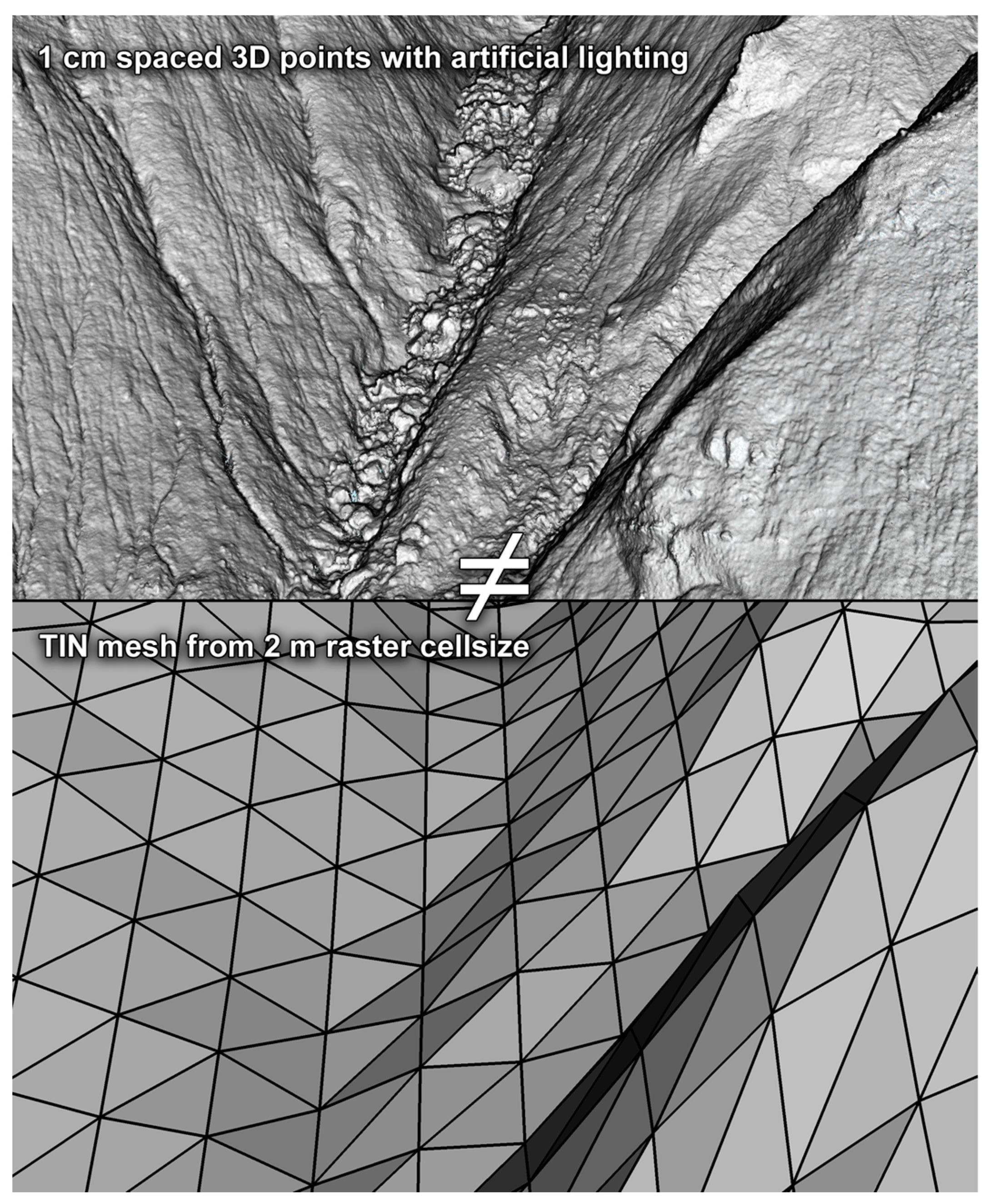
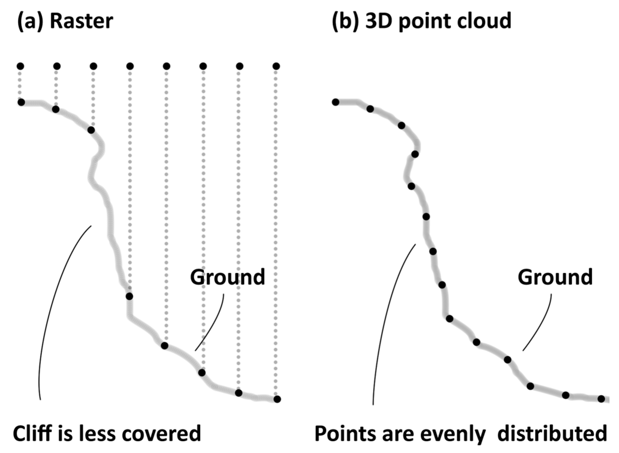
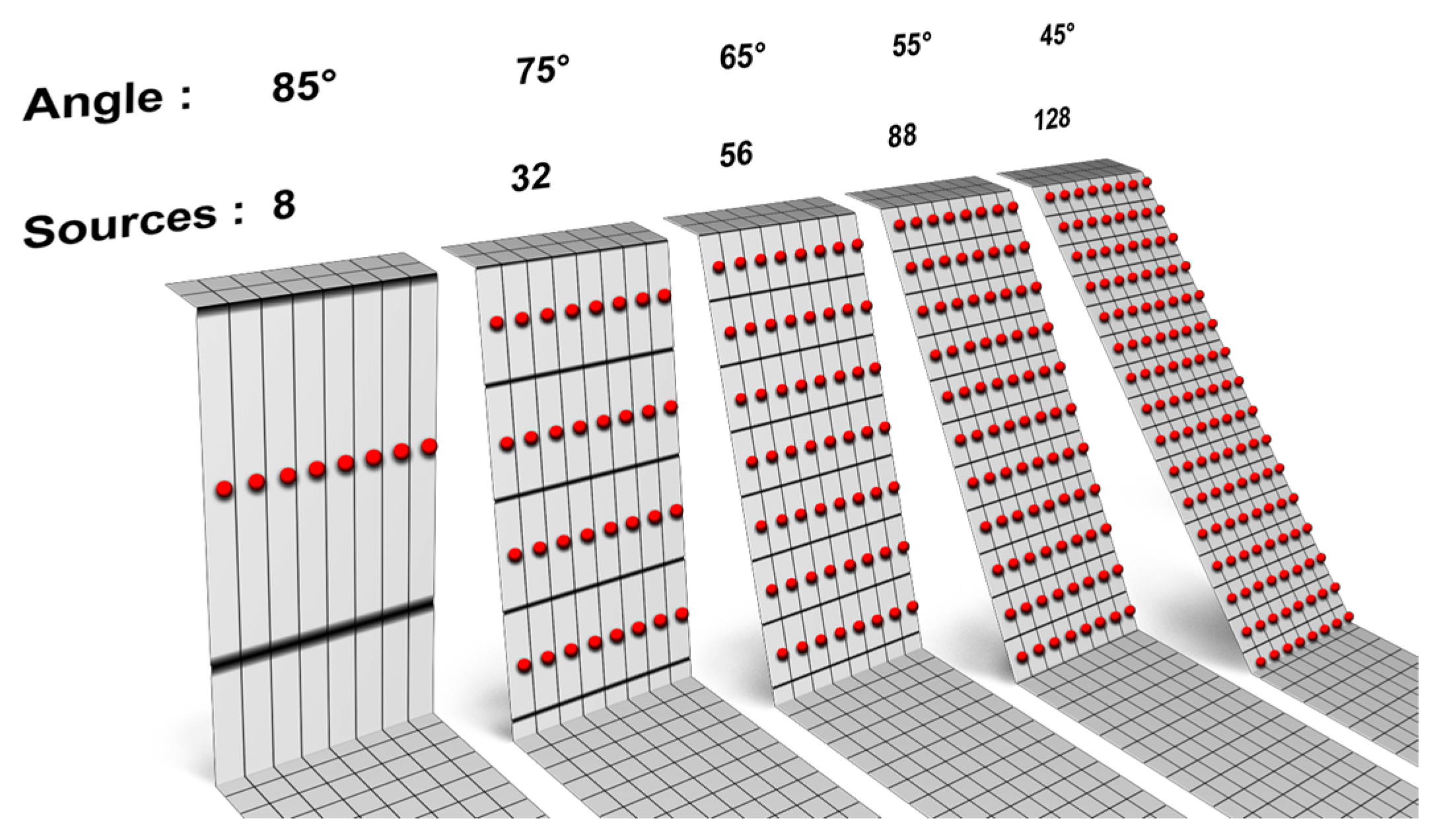
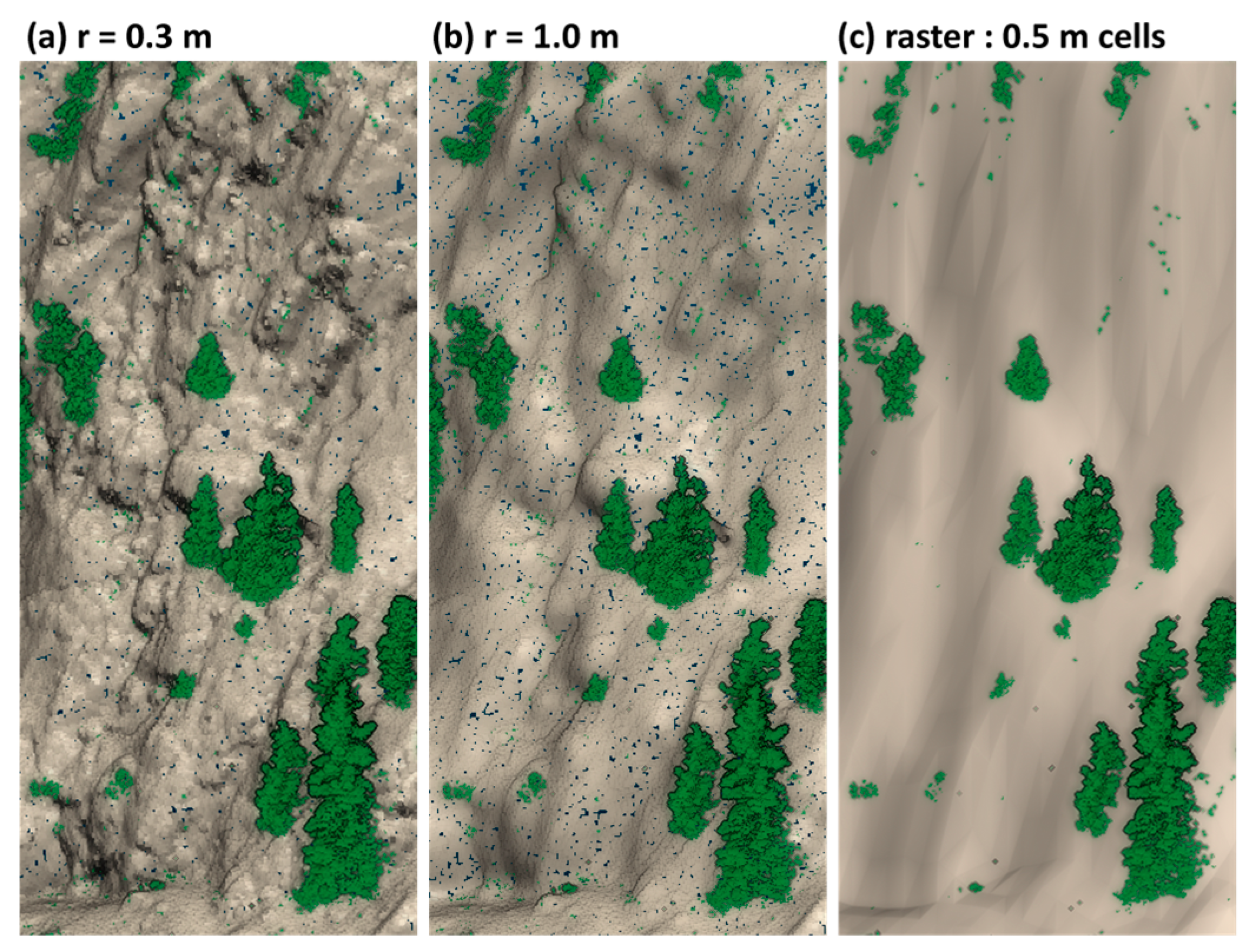
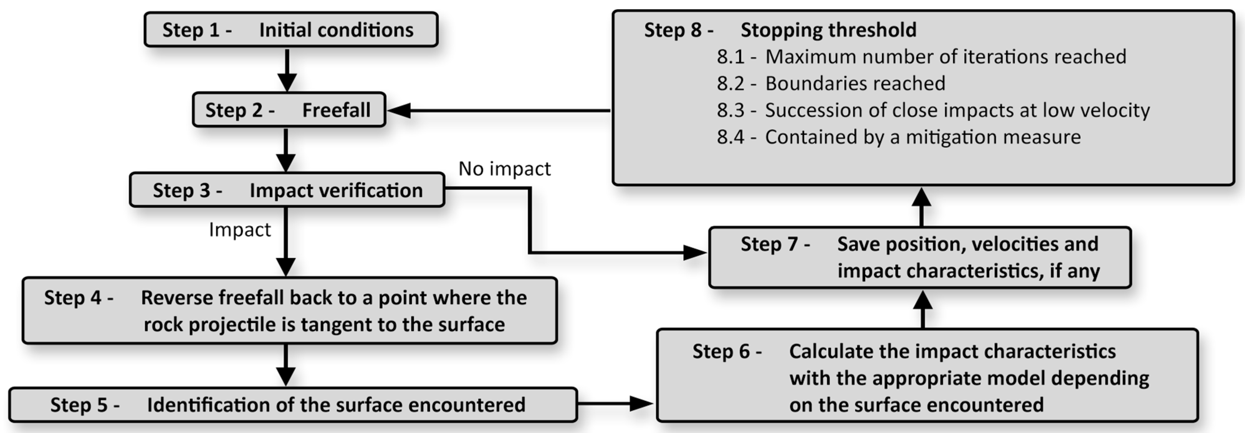
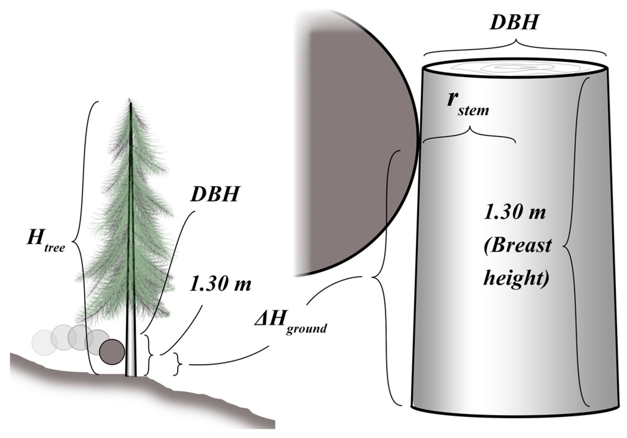
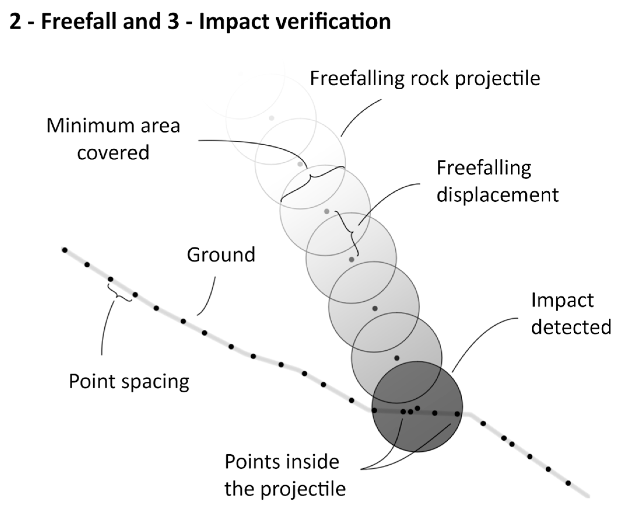
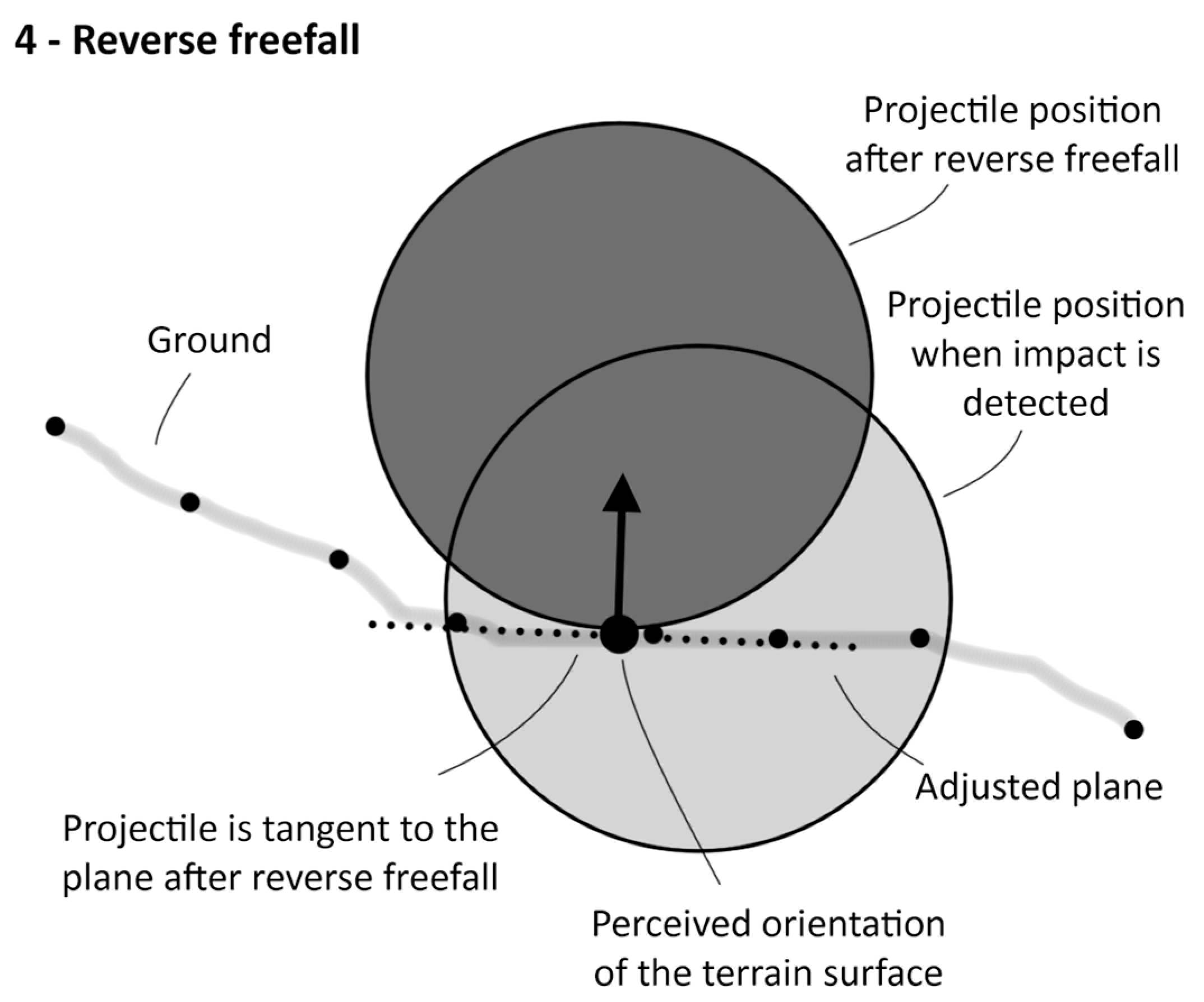
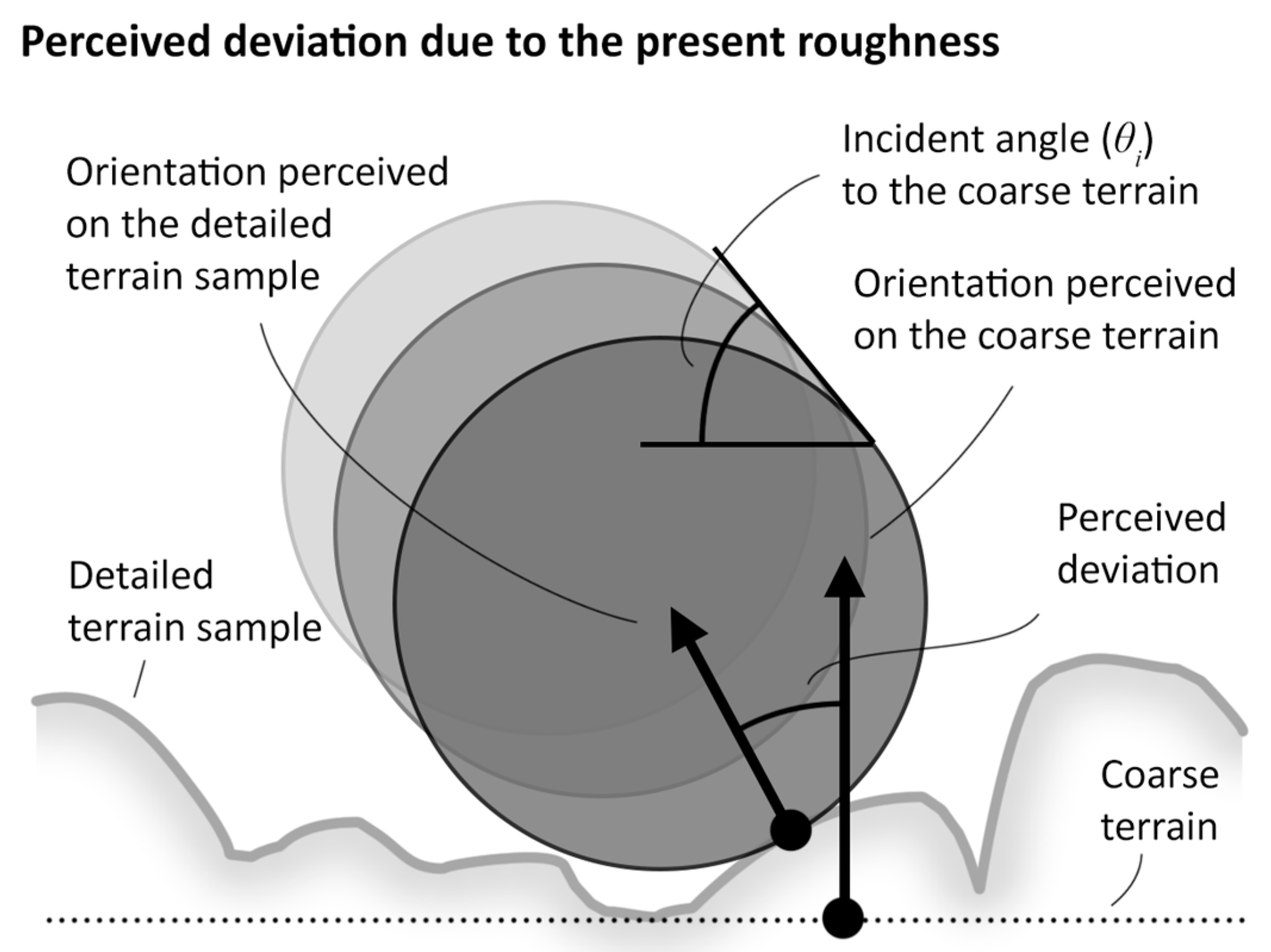
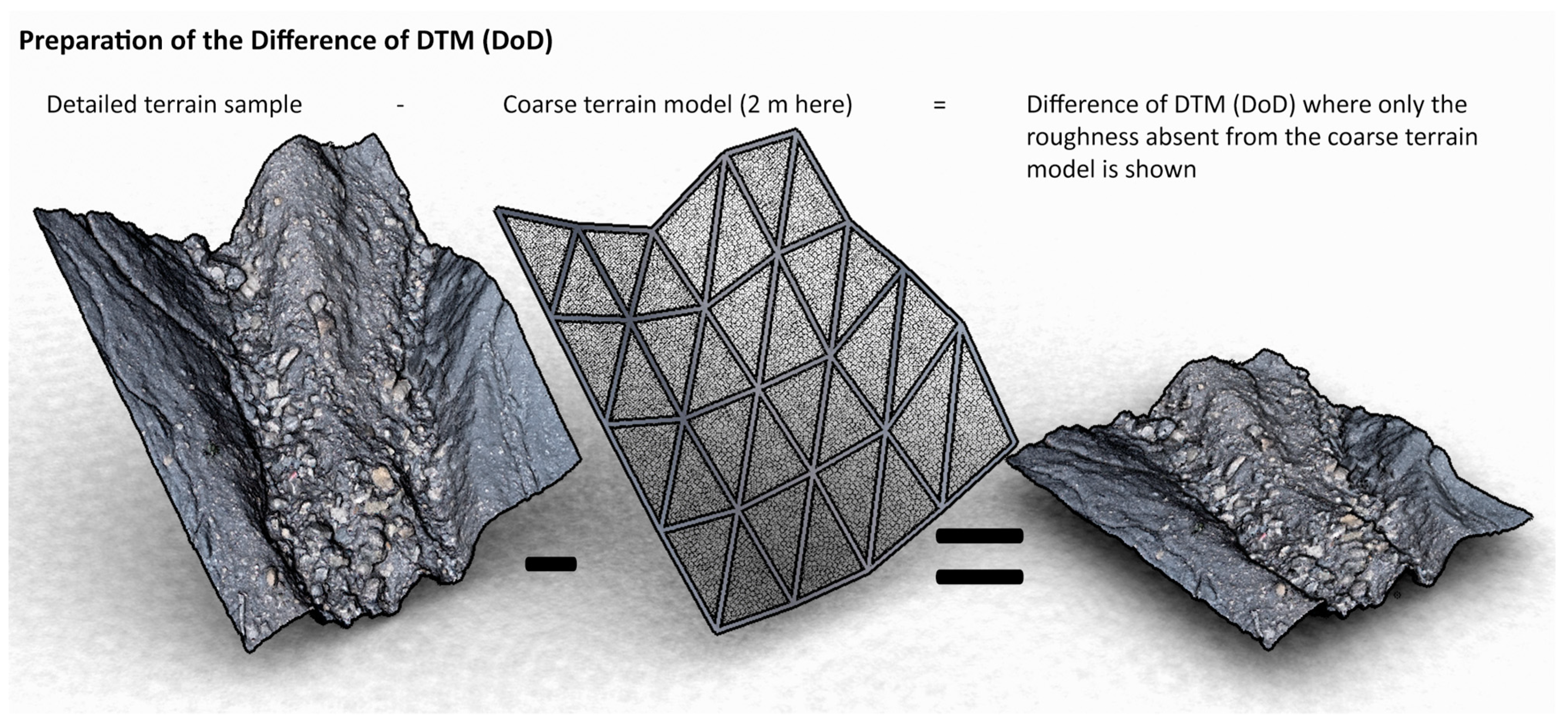
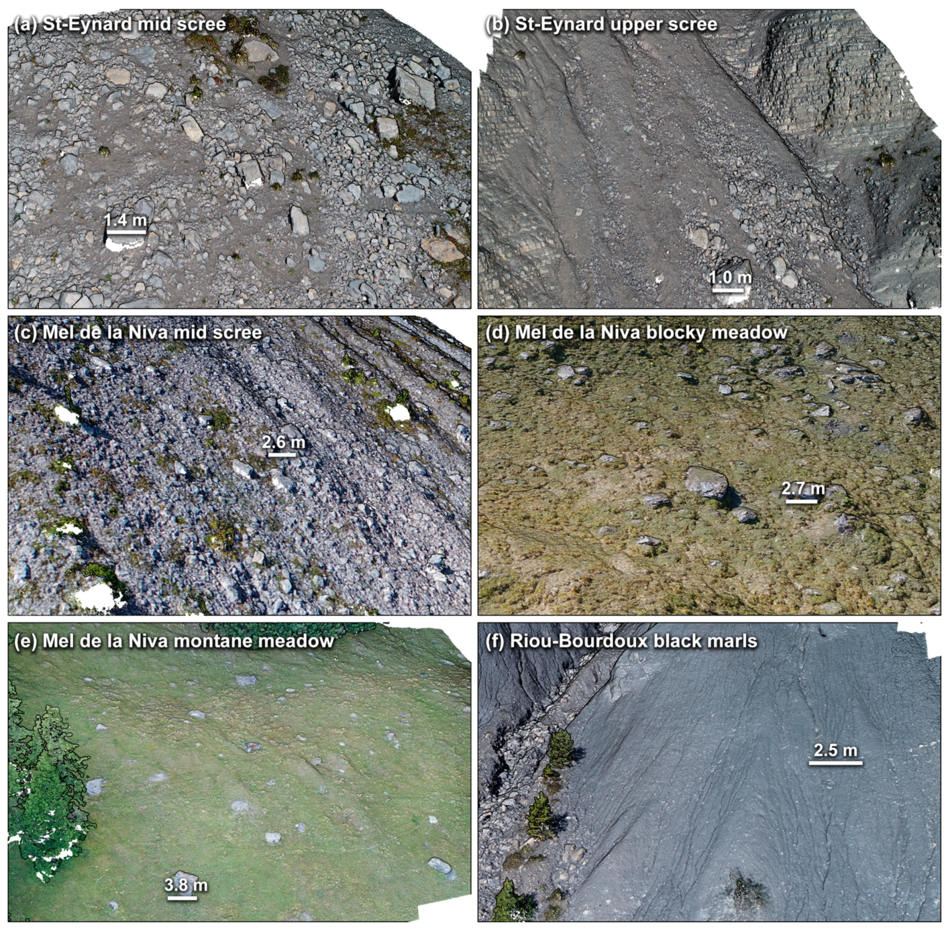
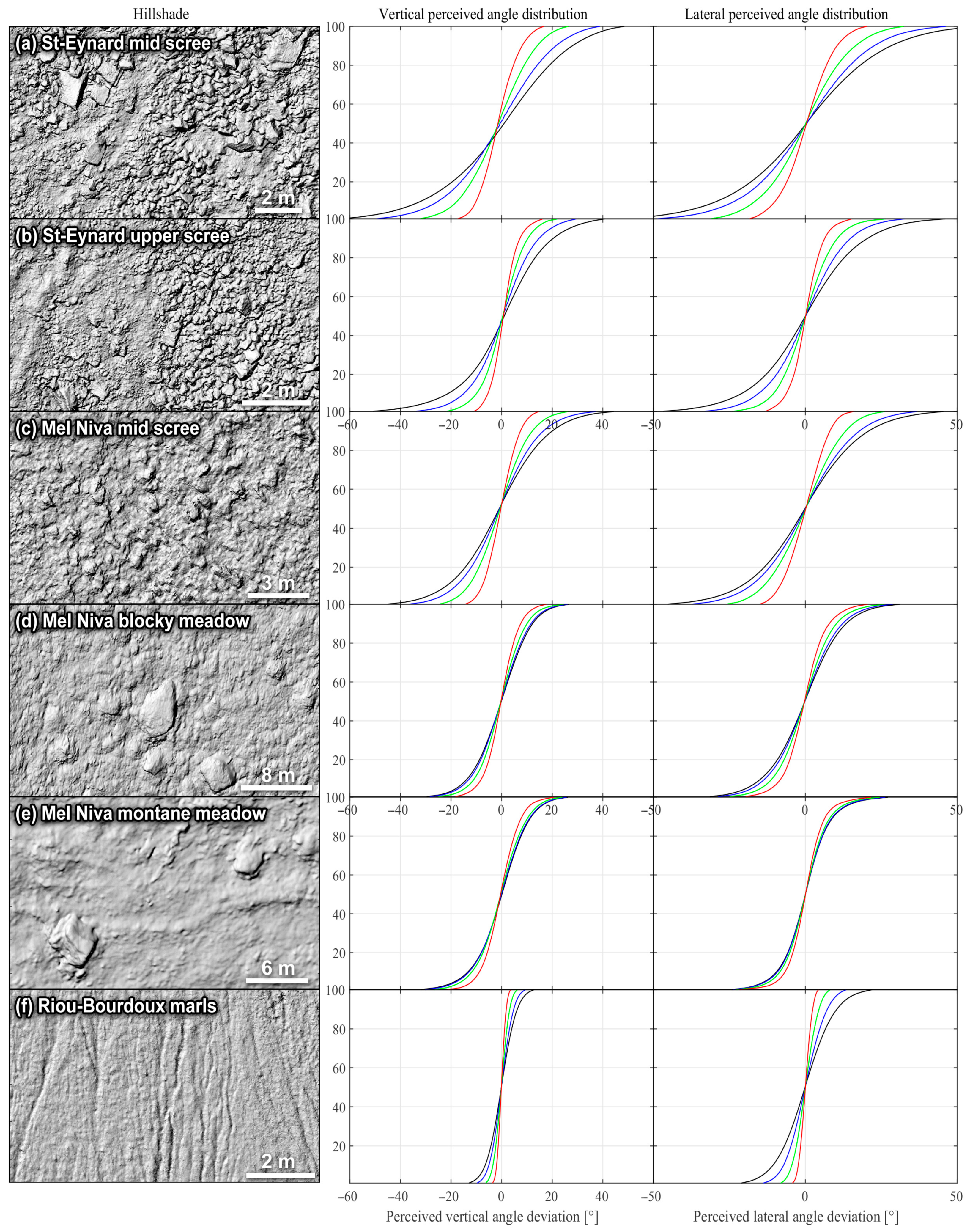
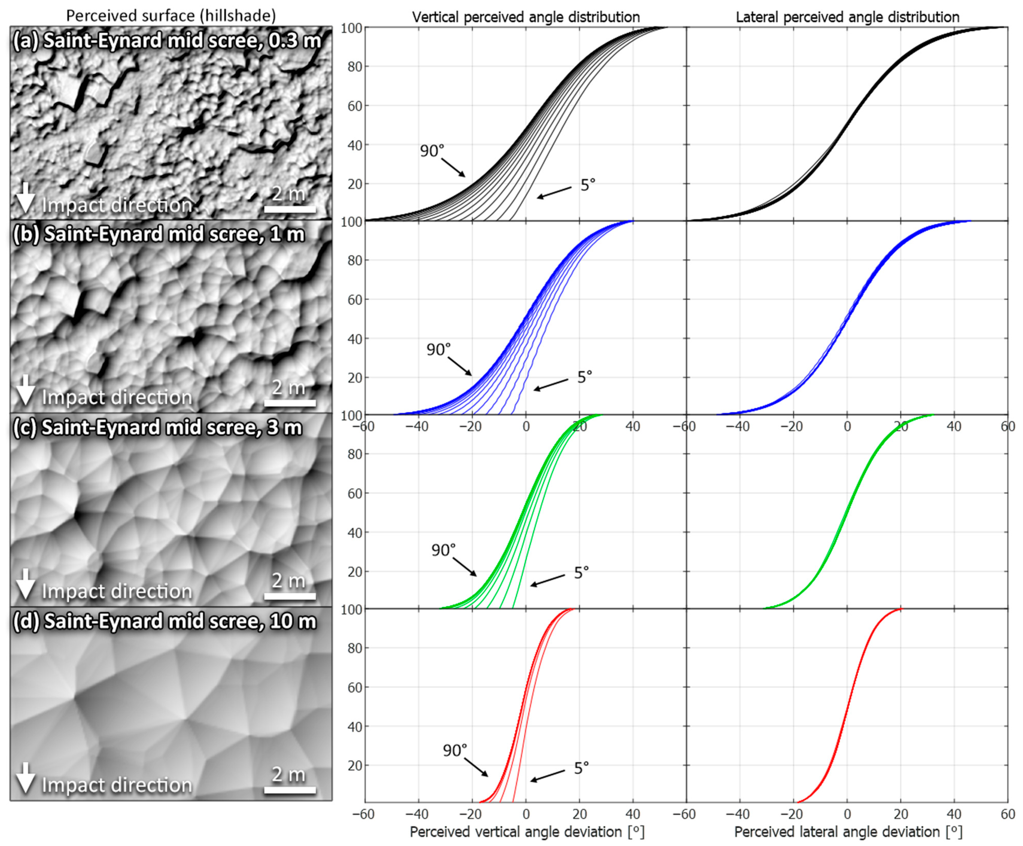
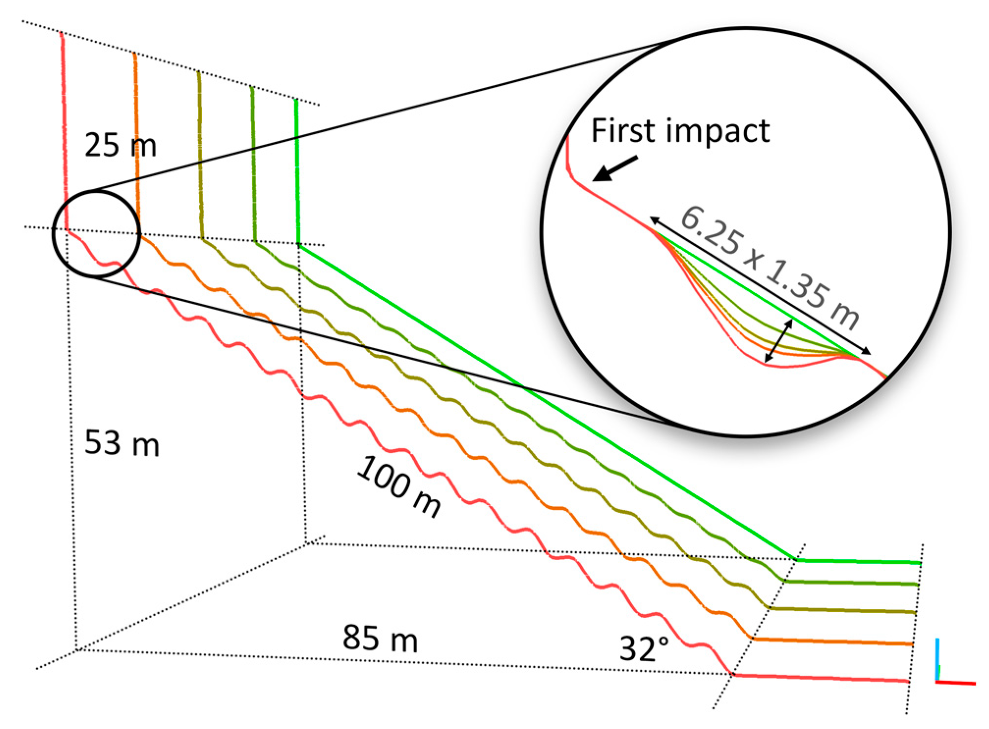
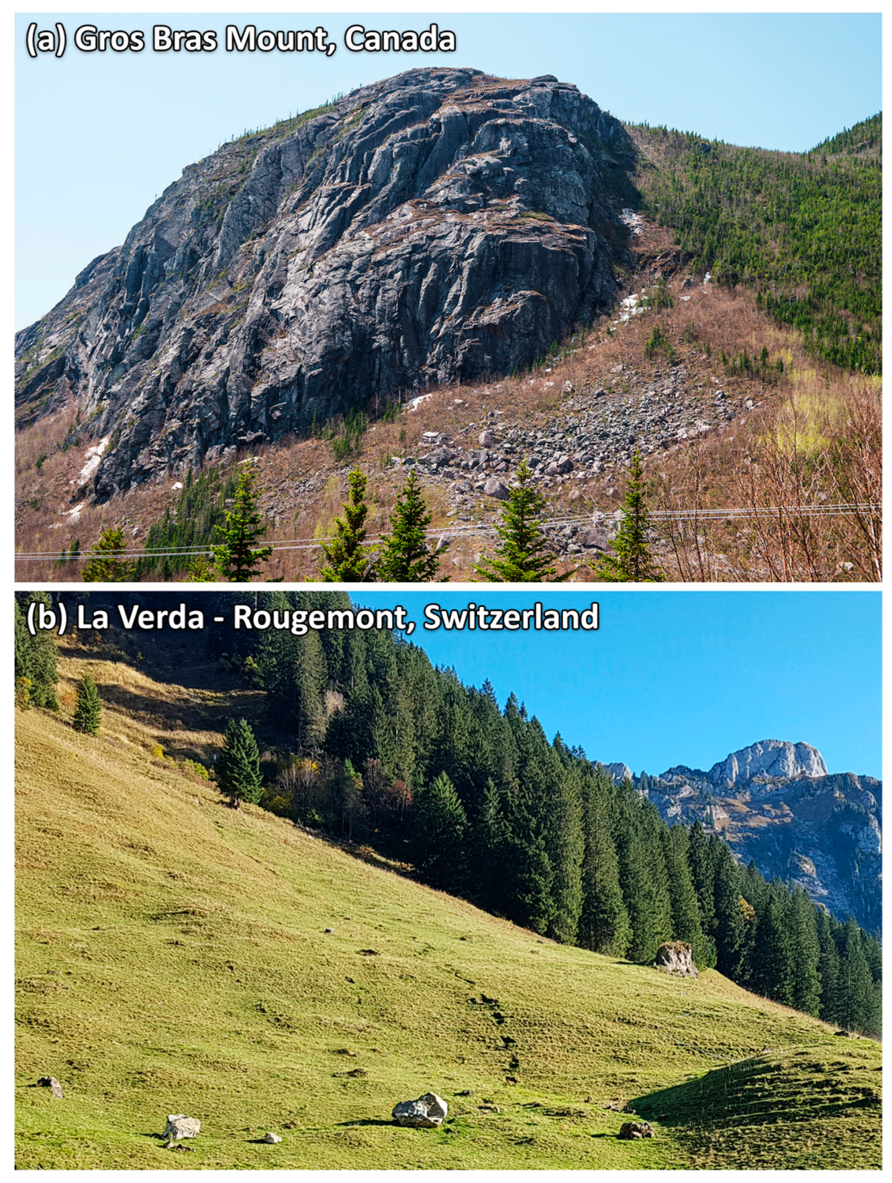
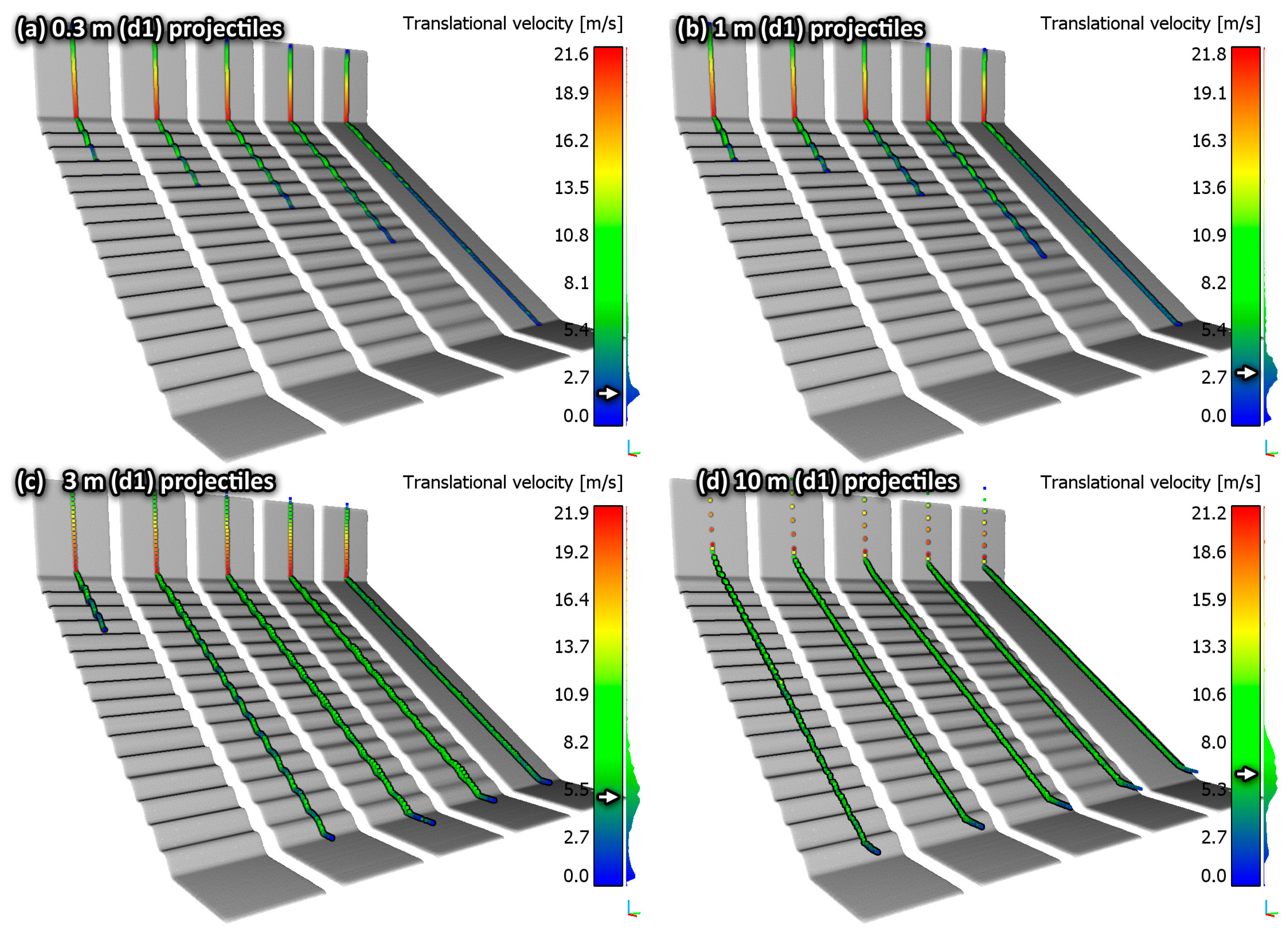
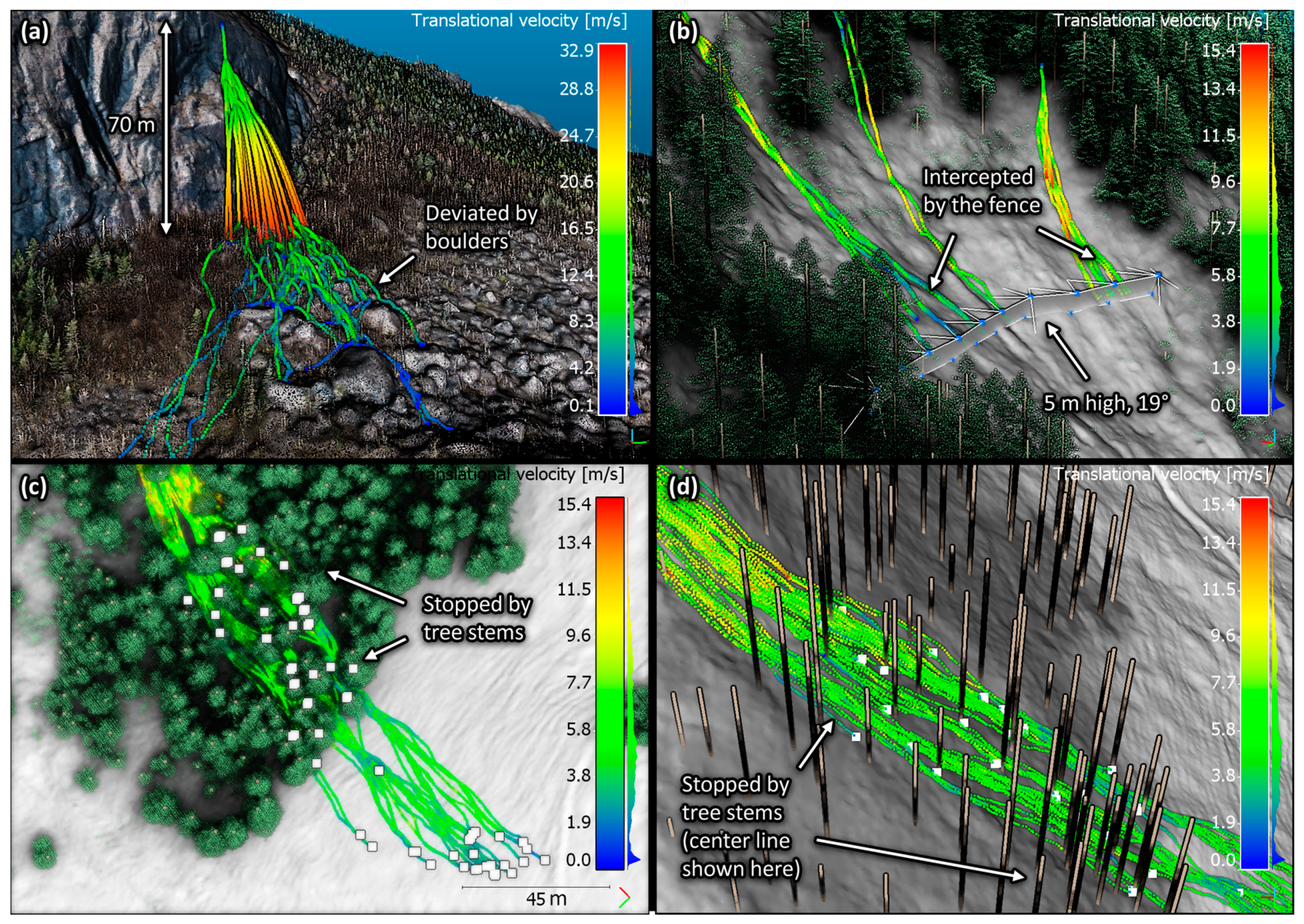
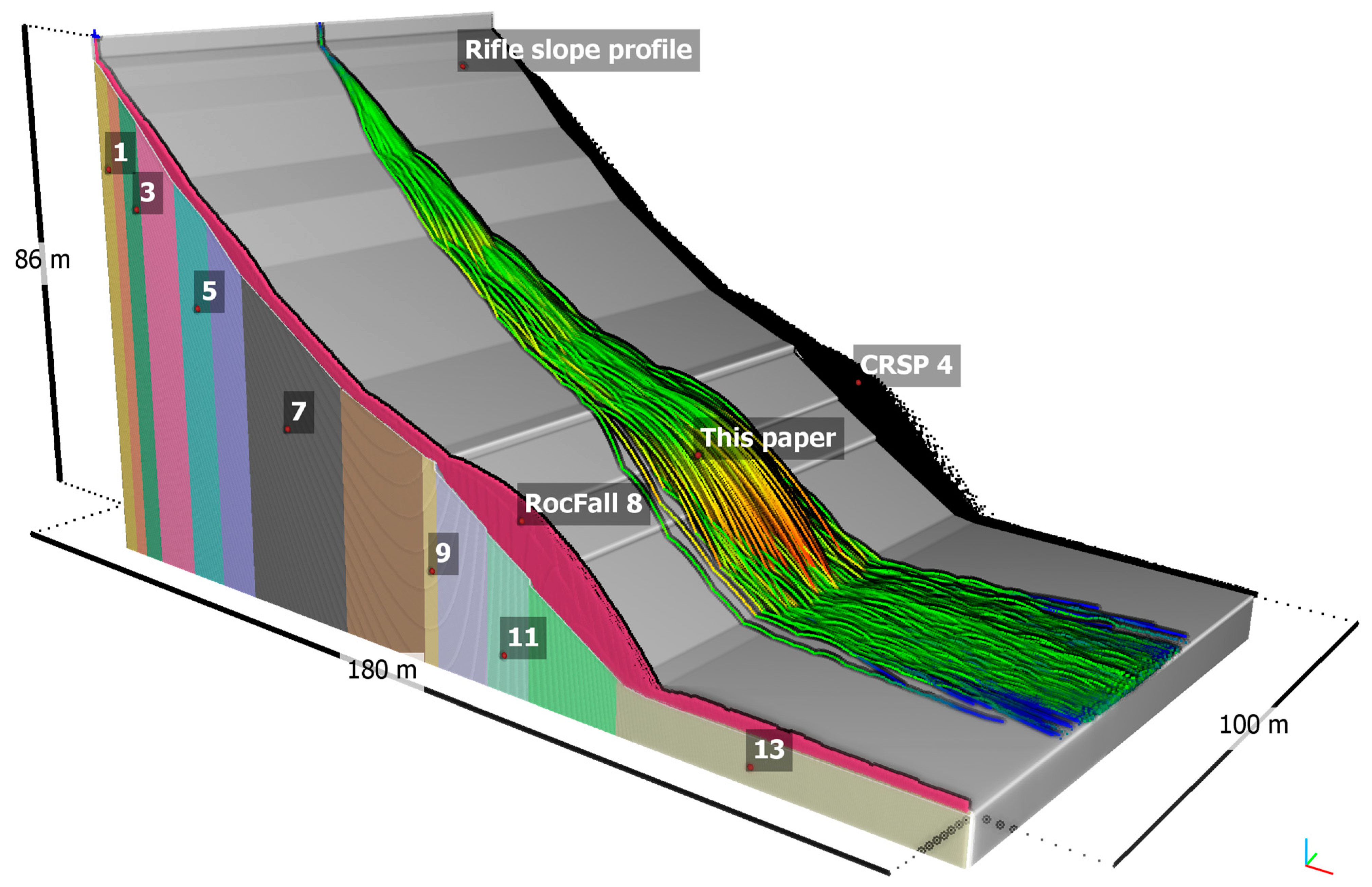
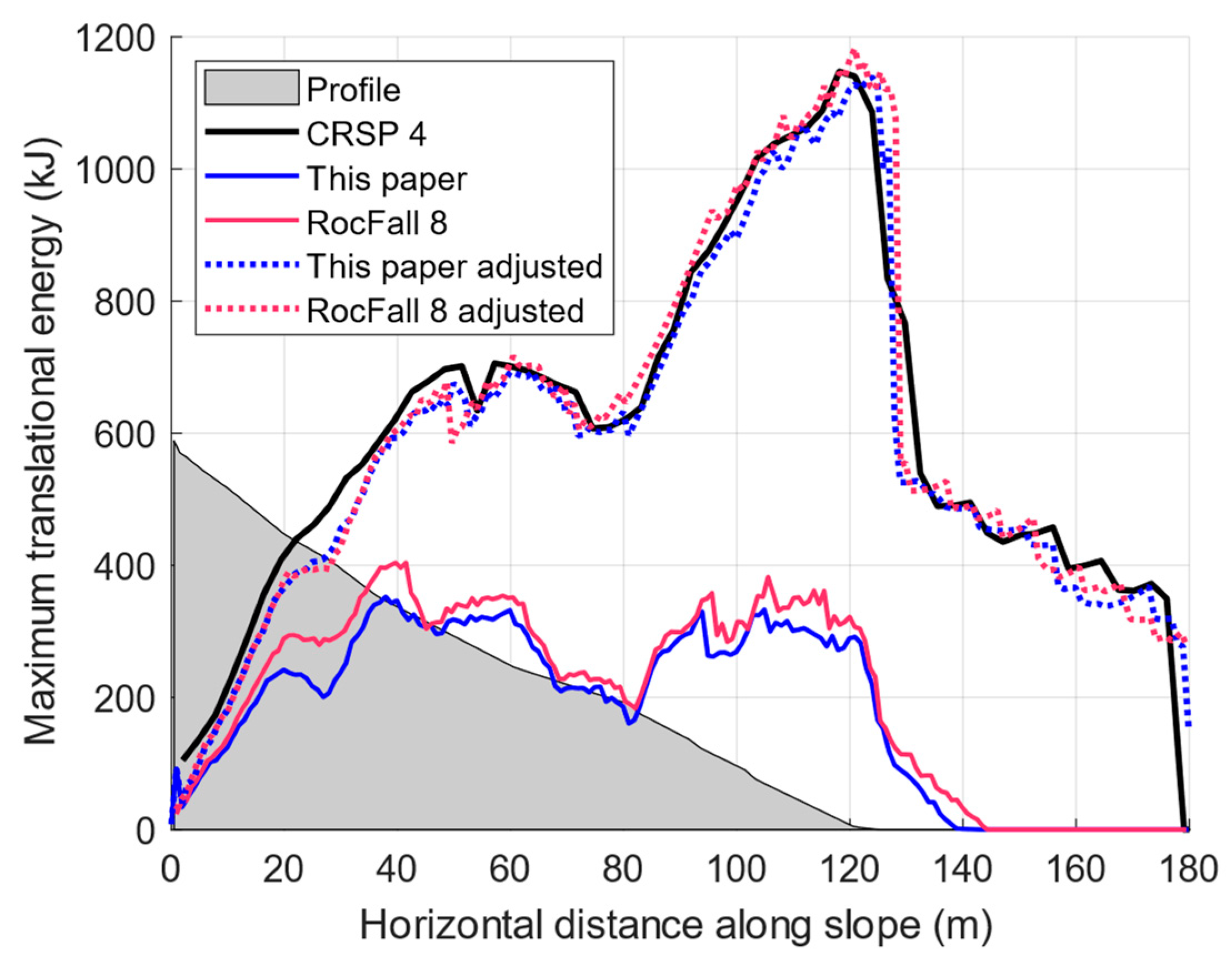
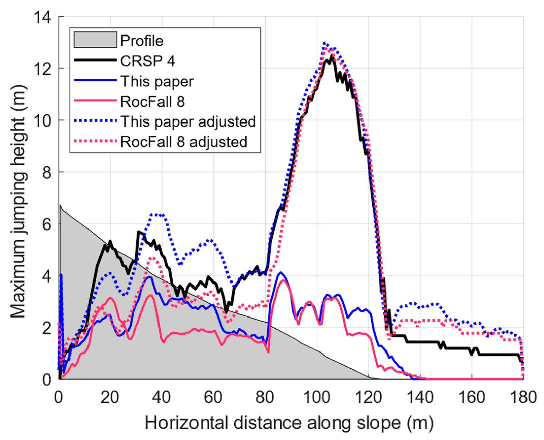
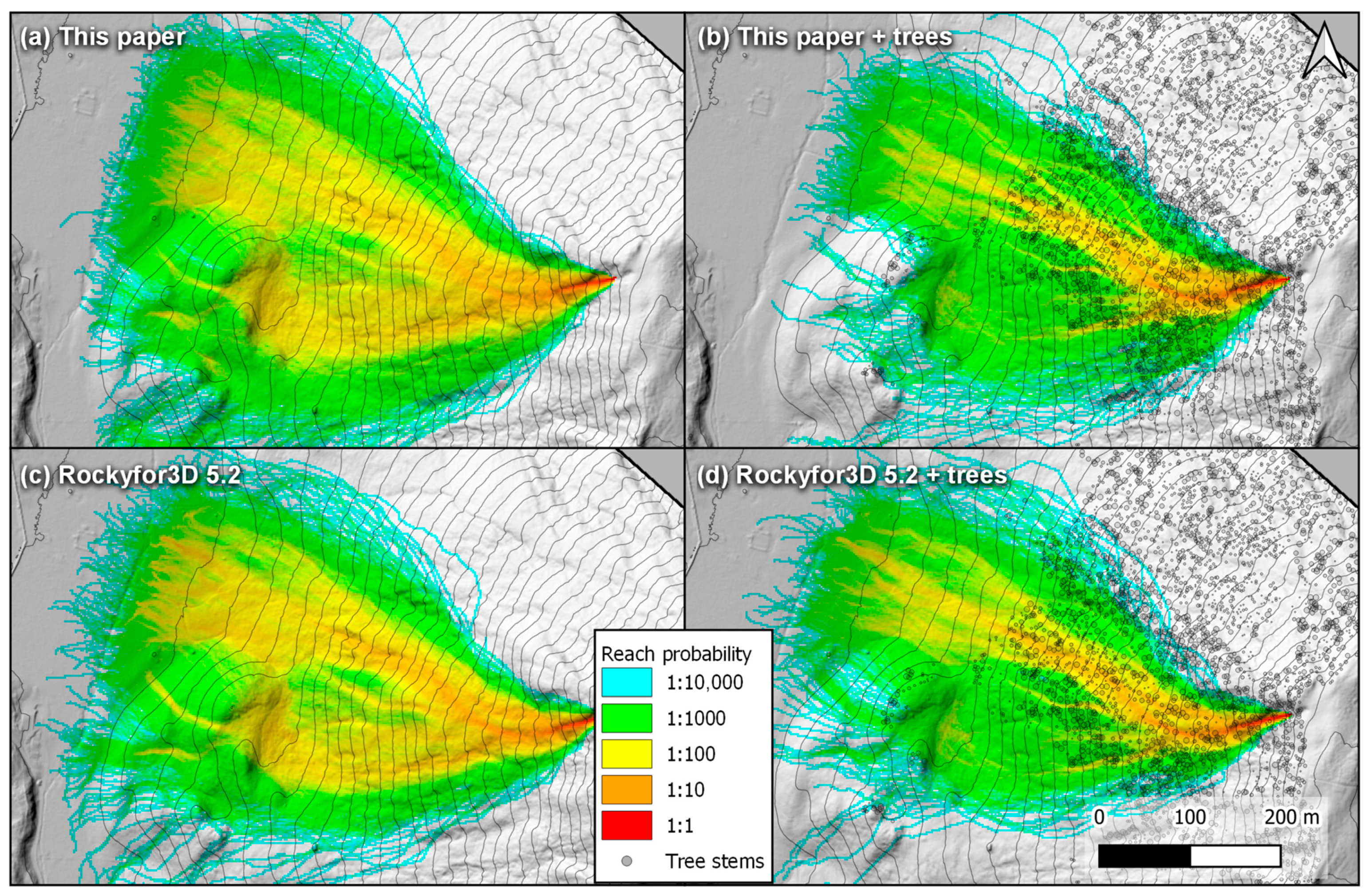
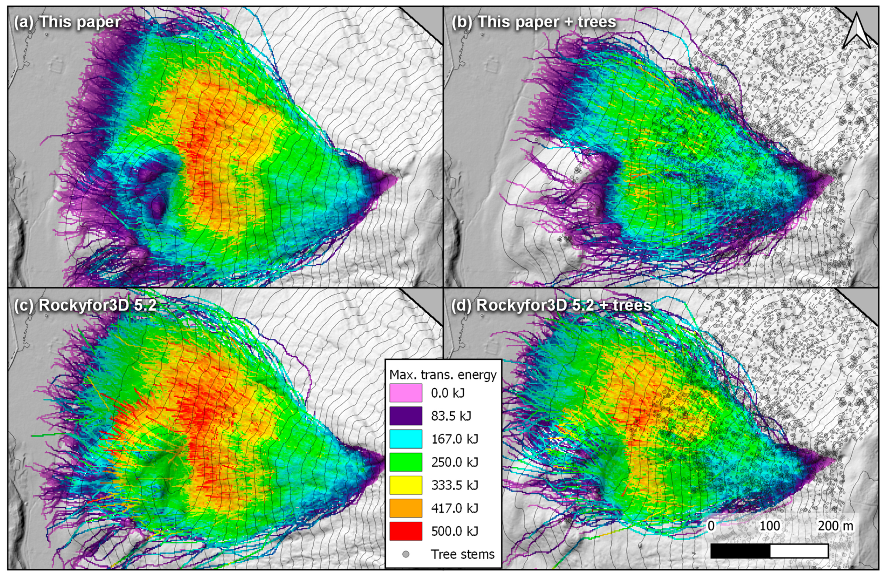
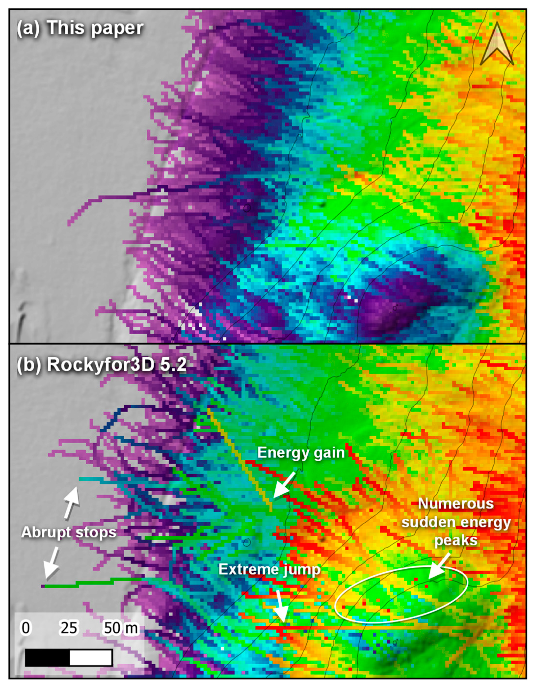
Table 1.
Probabilities for deviation occurring after an impact against a stem (after Dorren et al. [49]).
Table 1.
Probabilities for deviation occurring after an impact against a stem (after Dorren et al. [49]).
| Impact Configuration | Probability of Deviation |
|---|---|
| Frontal | |
| Lateral | |
| Scratch | |
Table 2.
Characteristics of the sites for the rockfall simulations.
| Parameters | Site 1a | Site 1b | Site 1c | Site 1d | Site 2 | Site 3 |
|---|---|---|---|---|---|---|
| Rn | 0.35 | 0.35 | 0.35 | 0.35 | 0.35 | 0.32 |
| Rn variability (Std Dev) | 0.04 | 0.04 | 0.04 | 0.04 | 0.04 | 0.04 |
| Rt | 0.85 | 0.85 | 0.85 | 0.85 | 0.85 | 0.83 |
| Rt variability (Std Dev) | 0.04 | 0.04 | 0.04 | 0.04 | 0.04 | 0.04 |
| d1 (m) | 0.3 | 1 | 3 | 10 | 1.9 | 1.9 |
| d2 (m) | 0.3 | 1 | 3 | 10 | 1.3 | 1.3 |
| d3 (m) | 0.3 | 1 | 3 | 10 | 0.9 | 0.9 |
| Mass (kg) | 38 | 1414 | 38 × 103 | 1414 × 103 | 3143 | 3143 |
| Point spacing (m) | 0.02 | 0.02 | 0.02 | 0.02 | 0.25 | 0.46 |
| Number of points (·106) | 10 | 10 | 10 | 10 | 1.8 | 1.9 |
Table 3.
Damping coefficients and artificial roughnesses used for the Rifle rockfall test site. The first 13 values are from Jones et al. [17]. They were replaced by the adjusted parameters shown on the bottom line for a second round of simulations with RocFall 8 and the proposed algorithm to obtain matching results with CRSP 4.
| Cell Number | θmax | Rn | Rt | |
|---|---|---|---|---|
| - | (m) | (°) | - | - |
| 1 | 0.12 | 11.3 | 0.25 | 0.82 |
| 2 | 0.18 | 16.7 | 0.32 | 0.84 |
| 3 | 0.24 | 21.8 | 0.32 | 0.84 |
| 4 | 0.61 | 45.0 | 0.32 | 0.84 |
| 5 | 0.24 | 21.8 | 0.3 | 0.84 |
| 6 | 0.24 | 21.8 | 0.3 | 0.84 |
| 7 | 0.24 | 21.8 | 0.3 | 0.83 |
| 8 | 0.30 | 26.6 | 0.33 | 0.82 |
| 9 | 0.24 | 21.8 | 0.33 | 0.82 |
| 10 | 0.43 | 35.0 | 0.34 | 0.84 |
| 11 | 0.37 | 31.0 | 0.34 | 0.84 |
| 12 | 0.24 | 21.8 | 0.34 | 0.84 |
| 13 | 0.12 | 11.3 | 0.34 | 0.85 |
| Adjusted | 0.18 | 16.7 | 0.28 | 0.98 |
Table 4.
Damping parameters based on slope thresholds used for the alpine slope near La Verda–Rougemont in Switzerland.
Table 4.
Damping parameters based on slope thresholds used for the alpine slope near La Verda–Rougemont in Switzerland.
| Slope | Soil Type | Rg70 | Rg20 | Rg10 |
|---|---|---|---|---|
| (°) | - | (m) | (m) | (m) |
| 0–2 | 3 | 0.03 | 0.03 | 0.03 |
| 2–7 | 4 | 0.05 | 0.05 | 0.10 |
| 7–25 | 4 | 0.05 | 0.10 | 0.20 |
| 25–45 | 5 | 0.00 | 0.05 | 0.10 |
| 45–90 | 6 | 0.00 | 0.00 | 0.00 |
Publisher’s Note: MDPI stays neutral with regard to jurisdictional claims in published maps and institutional affiliations. |
© 2021 by the authors. Licensee MDPI, Basel, Switzerland. This article is an open access article distributed under the terms and conditions of the Creative Commons Attribution (CC BY) license (https://creativecommons.org/licenses/by/4.0/).
Share and Cite
MDPI and ACS Style
Noël, F.; Cloutier, C.; Jaboyedoff, M.; Locat, J. Impact-Detection Algorithm That Uses Point Clouds as Topographic Inputs for 3D Rockfall Simulations. Geosciences 2021, 11, 188. https://doi.org/10.3390/geosciences11050188
AMA Style
Noël F, Cloutier C, Jaboyedoff M, Locat J. Impact-Detection Algorithm That Uses Point Clouds as Topographic Inputs for 3D Rockfall Simulations. Geosciences. 2021; 11(5):188. https://doi.org/10.3390/geosciences11050188
Chicago/Turabian StyleNoël, François, Catherine Cloutier, Michel Jaboyedoff, and Jacques Locat. 2021. "Impact-Detection Algorithm That Uses Point Clouds as Topographic Inputs for 3D Rockfall Simulations" Geosciences 11, no. 5: 188. https://doi.org/10.3390/geosciences11050188
Note that from the first issue of 2016, this journal uses article numbers instead of page numbers. See further details here.