Signal Processing of GPR Data for Road Surveys


1
Department of Engineering, Roma Tre University, Via Vito Volterra 62, 00146 Rome, Italy
2
School of Computing and Engineering, University of West London (UWL), St Mary’s Road, Ealing W5 5RF, UK
3
Applied Geophysics Laboratory, School of Mineral Resources Engineering, Technical University of Crete, 73100 Chania, Greece
4
Signal Processing for Telecommunications and Economics Lab., Roma Tre University, Via Vito Volterra 62, 00146 Rome, Italy
*
Author to whom correspondence should be addressed.
Geosciences 2019, 9(2), 96; https://doi.org/10.3390/geosciences9020096
Submission received: 20 December 2018
/
Revised: 2 February 2019
/
Accepted: 12 February 2019
/
Published: 19 February 2019
(This article belongs to the Special Issue Advances in Ground Penetrating Radar Research)
Abstract
:Effective quality assurance and quality control inspections of new roads as well as assessment of remaining service-life of existing assets is taking priority nowadays. Within this context, use of ground penetrating radar (GPR) is well-established in the field, although standards for a correct management of datasets collected on roads are still missing. This paper reports a signal processing method for data acquired on flexible pavements using GPR. To demonstrate the viability of the method, a dataset collected on a real-life flexible pavement was used for processing purposes. An overview of the use of non-destructive testing (NDT) methods in the field, including GPR, is first given. A multi-stage method is then presented including: (i) raw signal correction; (ii) removal of lower frequency harmonics; (iii) removal of antenna ringing; (iv) signal gain; and (v) band-pass filtering. Use of special processing steps such as vertical resolution enhancement, migration and time-to-depth conversion are finally discussed. Key considerations about the effects of each step are given by way of comparison between processed and unprocessed radargrams. Results have proven the viability of the proposed method and provided recommendations on use of specific processing stages depending on survey requirements and quality of the raw dataset.
1. Introduction
According to recent analyses [1], over 1.2 million human lives are lost every year worldwide due to road fatalities. It is therefore evident that road safety must be regarded as a major social issue. Thus, over the past decades, national and supranational institutions have set significant decreases in road mortality as a crucial target to pursue [2].
Within this context, decay of operations from standard conditions is regarded as one of the main sources of hazard for road users. Several studies have investigated the relationship between lack of maintenance and decay of road safety conditions at the network level [3,4,5]. Accordingly, required funds must be allocated on road maintenance to meet desired standards of serviceability and safety. As reported in [6,7], most of the funds available for highway infrastructure development are allocated to construction of newly-built infrastructures as opposed to management and rehabilitation of the existing asset. This is mostly due to three key factors [6]: (i) a general lowering of economic resources that may discourage governments and administrators to invest on new construction projects; (ii) the asset requirement to meet an increasing demand for mobility; and (iii) the ageing that affects existing road asset, especially infrastructures constructed between the 1960s and the 1970s.
In this framework, many efforts have been made to identify the most effective methodologies for health monitoring and assessment of road asset conditions. This is a crucial piece of information to support administrators in planning maintenance activities as well as in balancing operational, safety and economic concerns [8,9].
Nowadays, non-destructive testing (NDT) methods have become established in assessing actual requirements for maintenance of a transport infrastructure [7,10]. They allow to overcome many of the limitations of traditional inspection techniques. NDT methods generally involve a faster acquisition of data, more limited cost and a quasi-continuous collection of information on the inspected roads. Table 1 lists the most applied NDT methods in road surveying.
Within the range of available NDT methods, ground penetrating radar (GPR) is nowadays acknowledged as one of the most effective and powerful in road inspections. The main advantages of this method are the high flexibility of use and reliability of the outcomes [6]. Its working principle relies on the transmission and reception of short electromagnetic (EM) pulses in a given frequency band, which allow for an estimation of most of the physical and geometrical properties of the subsurface [28,29,30].
Use of GPR in road inspections covers a wide set of applications, ranging from quality assurance/quality control (QA/QC) inspections of new roads up to the assessment of the remaining service-life of existing infrastructures. Table 2 reports a list of main GPR applications for the inspection of roads.
In general, all of the above-mentioned applications require dedicated signal processing procedures to ease the result interpretation [28]. In this regard, it is known that signal processing is aimed at increasing the signal-to-noise (SNR) ratio of a received signal, providing a higher interpretability of the dataset [43]. However, the more intensive and sophisticated are the processing algorithms, the higher is the risk to compromise useful information in the source data and, therefore, to misinterpret the results.
Currently, standards for a correct management of GPR datasets collected on roads are still missing. This implies that successful processing and interpretation of data depends strongly on the expertise of the operators. This reveals a crucial issue, as processing errors can turn into systematic errors and affect the reliability of the whole database. However, the typical multi-layer structure of road pavement, along with a preliminary awareness of the construction materials of layers, make the GPR technology ideal for setting new monitoring standards in the field. This may contribute to lowering the risk of distortion of information.
Regardless of the specific processing algorithms used, several factors have to be considered prior to the elaboration of any data [6,44]:
- The quality of a final processing outcome is highly affected by the quality of data collection. Signals with very low SNR values within a raw dataset are most likely to produce misleading results after processing.
- The level of complexity of a survey goal, i.e., the level of detail required, affects generally the amount of work needed for processing.
- The cost of processing, typically quantified in terms of time required or human resources allocated, needs to be considered at an early stage, as these factors may significantly affect the final quality of an output in a GPR survey.
In view of the above considerations, it is worth to identify the main targets of a GPR inspection on roads as well as the survey protocols before any data collection stage. These factors must be considered beforehand against any processing-related strategy.
This paper presents an overview of conventional and advanced GPR data processing techniques for use as a guideline or as a good practice in road inspections. Algorithms are discussed for all the proposed processing steps. Main considerations about the effects of each processing step are given using a dedicated GPR dataset collected in a real-life flexible pavement. Finally, the importance of using detailed EM velocity models and multi-channel antenna systems in health monitoring of flexible pavements is discussed.
2. Ground Penetrating Radar
2.1. The GPR Technique
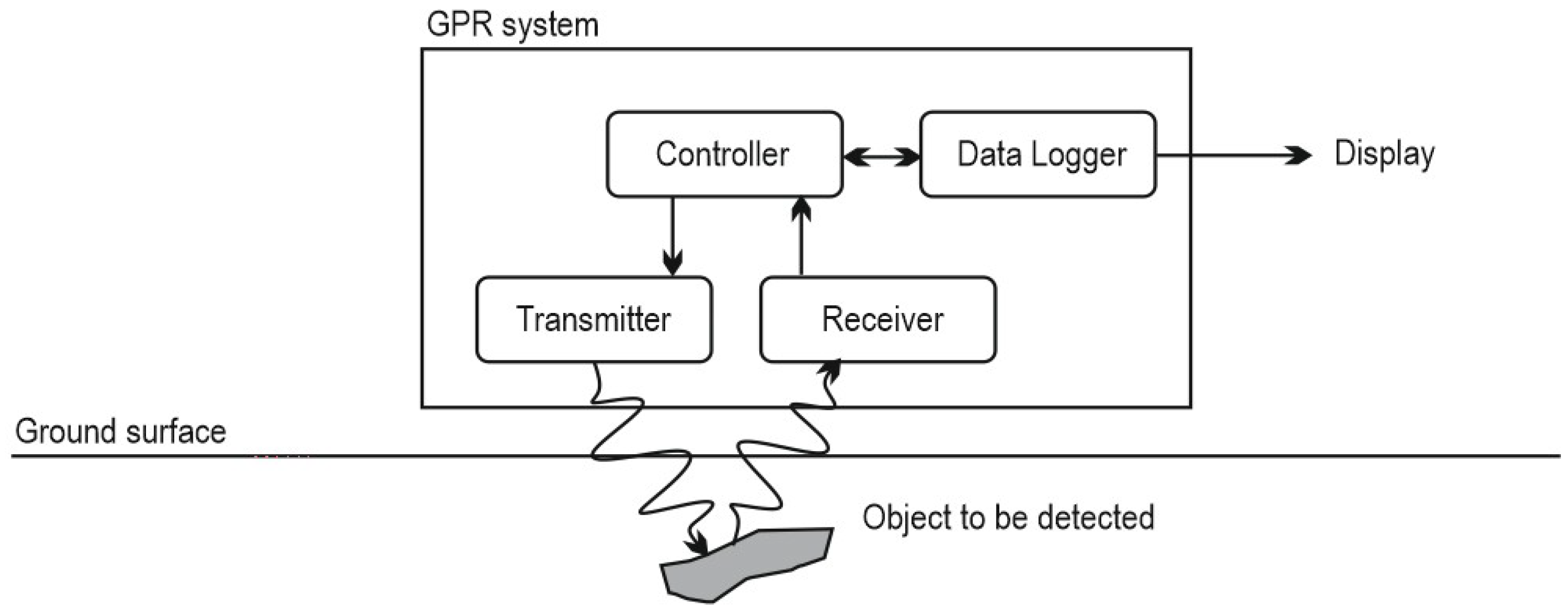
GPR is a geophysical EM method able to estimate information on the geometric and physical properties of the subsurface. A representation of a GPR system is reported in Figure 1.
In general terms, GPR works by emitting short pulses of high-frequency radio waves towards a target medium [28]. Transmission of an EM wave through a dispersive medium is defined according to the Maxwell’s theory. When an EM contrast is encountered, part of the energy is back-reflected, whereas the remaining part is refracted (i.e., transmitted to the following dielectric medium) until it meets a further dielectric contrast. This occurrence repeats until the wave attenuates. Electromagnetic properties of the investigated material can therefore be estimated by interpretation of the trend of reflection amplitudes against receiving time [28]. These properties are the relative permittivity ε, the electrical conductivity σ and the magnetic permeability μ. In more detail, ε and σ are found to highly affect the behavior of the travelling waves in terms of velocity and attenuation, respectively. In most cases, the magnetic permeability μ is considered to equal the free-space magnetic permeability μ0 for all non-magnetic materials.
The overall depth of penetration and vertical resolution of a signal depends on several factors. These mostly relate to the technical specifications of the system, e.g., the central frequency, as well as to the physical properties of the medium investigated. The central frequency of GPR systems commonly used in road inspections is typically in the range 500–2500 MHz [6].
2.2. Main Survey Configurations
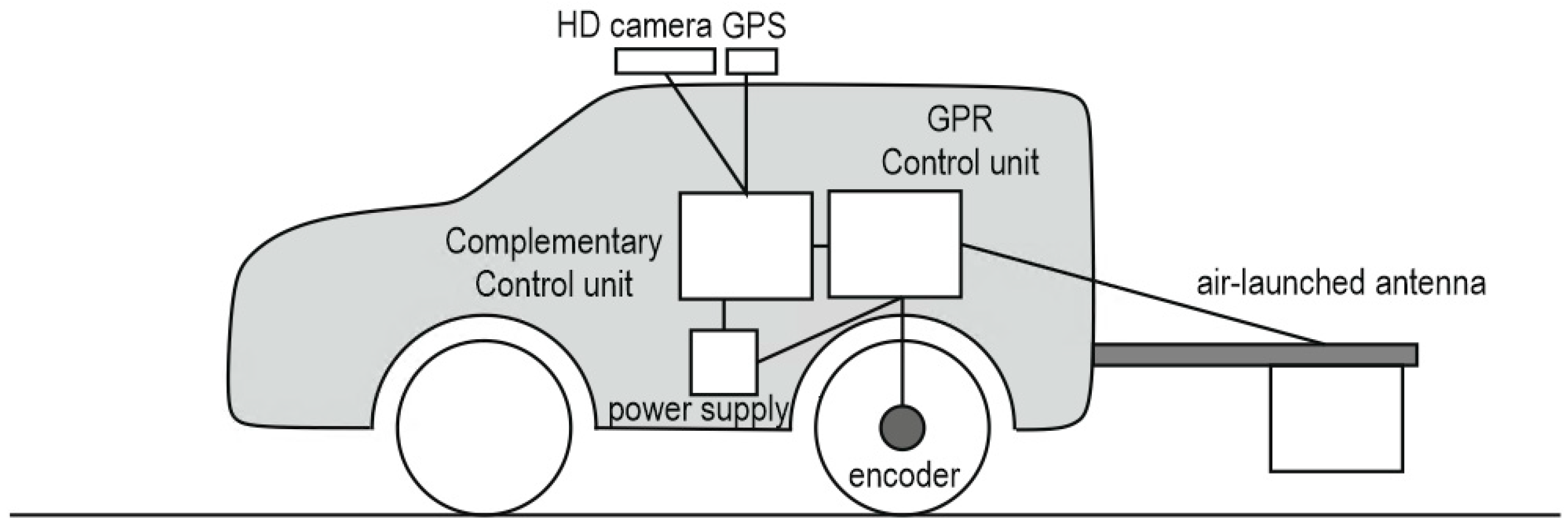
In general, road surveys with GPR are carried out by means of impulse radar systems [45]. These systems, as opposed to stepped-frequency continuous-wave (SFCW) radars, generate very short pulses around a fixed central frequency. Moreover, GPR configurations for inspection of roads are most commonly air-coupled antenna systems. These are attached to an inspection vehicle and work suspended in the air at a height from the ground varying from 0.30 to 0.50 m. The main advantage of these systems over ground-coupled antenna systems is the rapidity in the acquisition of data. Hence, they are highly efficient with a very limited impact on car traffic [46]. In addition, as air-coupled antenna systems do not produce EM pulses within the road surface (as it applies for ground-coupled antenna systems), a reference propagating waveform (e.g., a waveform acquired from a reflection on a metal plate) can be used for interpretation and deconvolution, if required. This means that a reference waveform can be used for amplitude analysis of the EM reflections within the GPR dataset or for the calculation of an inverse filtering operator, respectively. The main drawback of air-coupled antenna systems is the limited penetration, as most of the transmitted energy is lost due to the high dielectric contrast between the air and the road surface. A typical GPR system configuration for road monitoring is illustrated in Figure 2.
Accessory equipment is often coupled to standard equipment for integration of GPR data with additional information. The most used complementary pieces of equipment are Global Position Systems (GPS), for an accurate localization of the GPR traces, and high-definition Video Cameras. These allow for a more comprehensive interpretation of the EM data by observation of surface and antenna surrounding conditions. Further devices have been reported to pair with GPR depending on the specific goal of a road survey. Among the most acknowledged in the literature, drilling systems, infrared thermography cameras [47,48] and laser scanners/profilometers [49] are worthy of mention.
3. The GPR Dataset
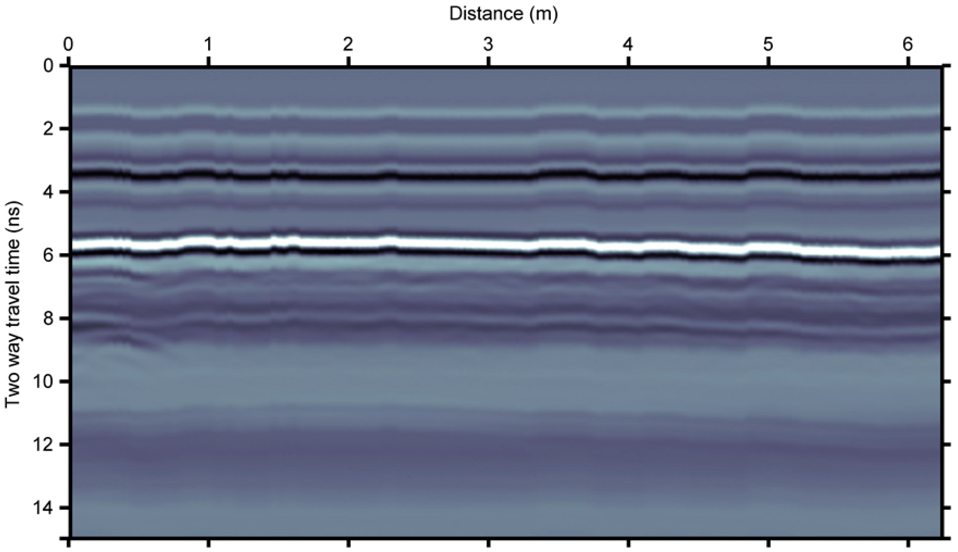
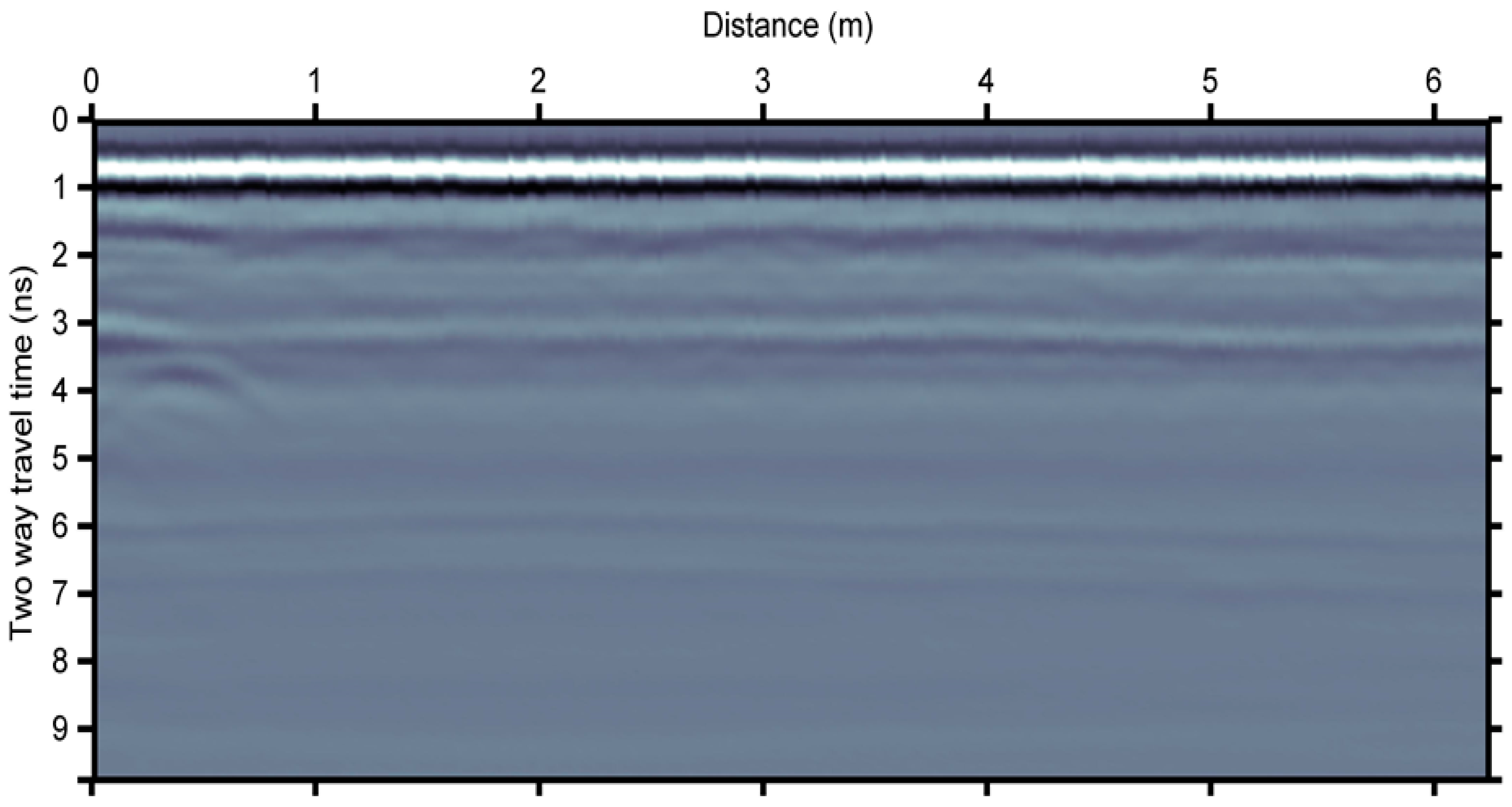
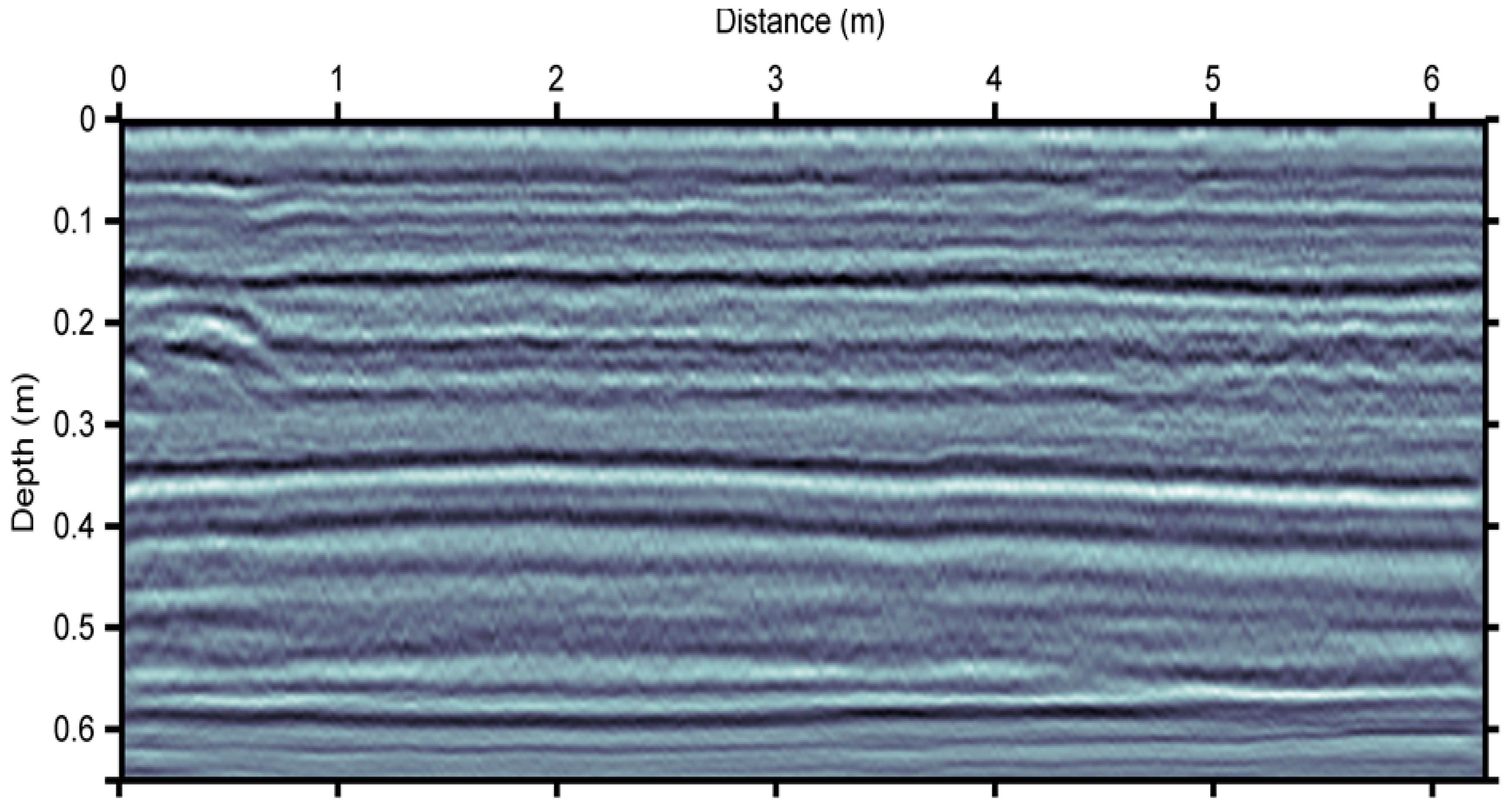
Practical examples are discussed in this paper for various processing steps, with reference to a real data acquisition. Data were collected on a flexible pavement of a rural road located in the District of Madrid, Spain, using the HI-Pave HR system, manufactured by IDS Georadar S.p.A., equipped with an air-coupled horn antenna type. The nominal frequency of the antenna is 2000 MHz, and the time interval was set as 0.0293 ns (512 samples per 15 ns). As transmitter and receiver are very close, they were considered to be approximately at the same position (i.e., a monostatic configuration). The horizontal resolution was set at 0.0208 m and the antenna apparatus was placed at 40 cm above the road surface. An encoder was installed on a wheel of the inspection vehicle to track the exact distance covered by the antenna during the survey. The inspection speed was maintained relatively constant, around a value of 50 km/h, on the average. The raw GPR data are shown in Figure 3.
4. The Processing Protocol
The sequence reported in this Section is intended as a general protocol for processing GPR data collected on flexible pavements. Nevertheless, some applications may require use of a different number of steps depending on the specific goal of a survey. In addition, different processing protocols may be required for a minor set of case scenarios. For the sake of brevity, only limited information on the theoretical background behind the discussed processing steps are reported in this paper. In this regard, more details can be found in [50,51].
A list of processing steps discussed in this paper is as follows:
- Raw signal correction
- ○
- Removal of incoherent traces and replacement by interpolation
- ○
- Time-zero correction
- ○
- Elevation correction
- ○
- Energy normalization
- Lower frequency harmonics removal
- Removal of antenna ringing
- Signal gain
- Band-pass filtering
- Special processing steps
- ○
- Vertical or time resolution enhancement
- ○
- Migration or lateral resolution enhancement
- ○
- Time-to-depth conversion
Processing flow diagrams are not included in this paper as these are widely reported in the literature [6]. The reader must consider that processing steps discussed in this paper are listed based on the typical sequence for applications on data. Only gain is applied after a few processing steps for improving data visualization, as this step should always be applied at the end of a processing sequence.
The term “wavelet” is used throughout all the manuscript to denote the incident EM wave, or incident waveform or the reflection waveform as it is used in other similar studies. The algorithms used in this paper to demonstrate the viability of the processing were implemented in Matlab. The reason for this is that commercial software tools (or “black-box” software) do not usually provide any details on the implementation process. On the opposite, use of in-house numerical codes allows to have a full management of the output expected.
4.1. Raw Signal Correction
Raw signal correction is a preliminary stage of the overall processing protocol. This is compulsory to ensure highly reliable interpretations within the procedure to apply at the following stage [6].
Potential errors occurring during the survey at the setting of the test system need to be adjusted. Secondly, errors occurring during testing must be accounted for. The most common operations are listed below.
4.1.1. Removal of Incoherent Traces and Replacement by Interpolation
It is a common practice to remove from the raw dataset single traces not coherent with the surrounding ones. A linear interpolation is then usually performed to cover the gap information.
This occurrence is not rare in road inspections, as the excessive speed at the time of data collection is one of the main sources of incoherent traces. Specifically, this is most likely to be observed for travelling speeds higher than 70–80 km/h, when the maximum sampling frequency is exceeded and asynchrony between the actual position of a GPR trace and the scanning distance recorded by an odometer can generate. However, it is worth to remind that a too frequent trace replacement by interpolation methods may cause a loss of important information (e.g., reflections from voids or wet spots) from the raw dataset. In addition, it is recommended for a user of a commercial software to be aware of the type of default interpolation used in the processing. This is crucial to avoid any possible mislead at the signal processing stage as well as to improve data interpretation.
4.1.2. Time-Zero Correction
It may occur that the direct wave arrival times (time-zero) are not horizontally aligned along the main longitudinal scanning direction. This is most likely due to the non-stable temperature of the system and/or to damaged cables and connections. For road inspections conducted with an air-coupled antenna, this occurrence is typically exacerbated by the bouncing of the antenna support, due to the high-speed of acquisition. This causes the default height of the antenna to vary along the inspection length [52,53].
A correction for this occurrence is to cut the direct waves by removing the first arrivals and the air layer between the antenna and the asphalt surface. It is required to define a reference threshold for this removal to move all the traces at the same time-zero position. Various thresholds have been reported to work effectively in the literature: (i) the first break (i.e., the time where the waveform starts the oscillation); (ii) the first positive or negative peak; (iii) the zero-amplitude point between the first positive and negative peaks; and (iv) the average amplitude point between the positive and negative peaks [6,54]. The choice of the first break is usually on users with a seismic background and it is based on the convolutional model. This means that the recorded waveform (trace) is the outcome of the convolution of the ground response (spikes representing reflectivity series) with the waveform sent by the antenna into the ground. The convolution process turns out to provide a delay of the waveforms and their oscillation generates at the point position of the spike. Hence, if symmetrical waveforms are assumed, the larger peak (positive or negative) is placed at a recorded time equal to half of the duration of the whole waveform after the spike. Other options are to find a best trade-off depending on the easiest choice for the data processor. Applications of the above thresholds have proven advantages and drawbacks, depending on the features of the investigated medium as well as the GPR systems. As an example, use of the first break can be made only for waveforms with a changing shape in time, as the origin point of the waveform is a required information. This approach can be therefore used in most of the cases, although it is the most difficult one to employ for an accurate and stable picking of all the traces. On the contrary, the first positive peak holds the advantage of being easily detectable, although it might be unsuitable and inaccurate for deeper horizontal reflections. This is due to the alteration of the dominant waveform’s shape when signal dispersion is medium to high at late times.
In addition, it is worthy of mention that all the threshold choice methods are expected to work effectively for road monitoring data, as the dispersion is typically not as high as in other application areas. On the opposite, the first break should be used as a reference picking method in case high values of dispersion are observed.
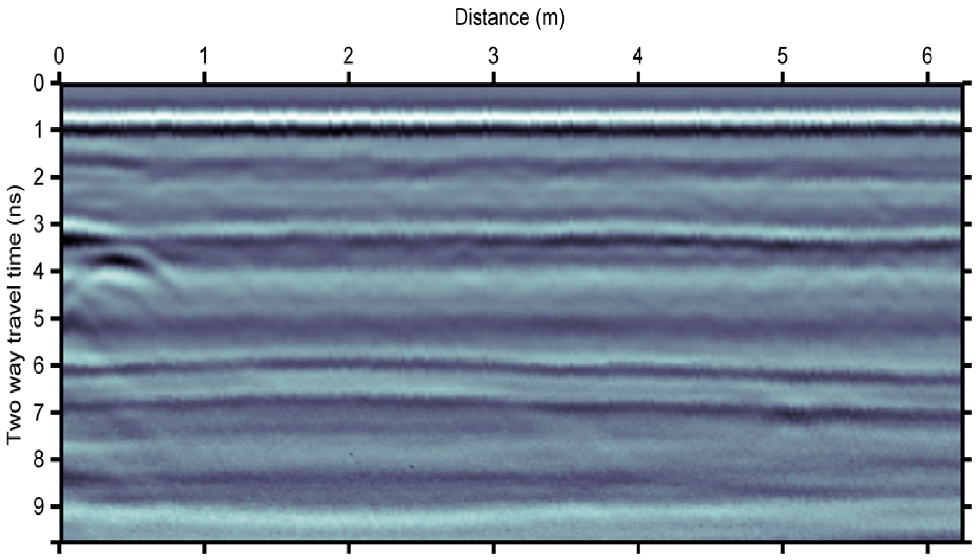
Figure 5 shows the effects of the application of the time-zero correction step to the raw signal reported in Figure 3. The first break of the road surface reflection was here used as a reference, as the first break of the road surface reflection was relatively evident to be picked. Moreover, this specific method allowed to avoid inaccurate picking for the rest of the horizontal reflections within the pavement structure. As a result of the application of this method, the road surface reflection is now the first reflection imaged within the GPR section with a horizontal arrangement, denoting a constant offset between the GPR device and the surface.
4.1.3. Elevation Correction
When the terrain is not levelled, reflections and hyperbolas are not sufficiently imaged. This issue can be sorted by applying corrections for the topography in the GPR section. Nevertheless, when the terrain is highly irregular, application of topography corrections may return unreliable GPR images. To this effect, time-zero correction must be applied before the elevation correction step.
It is worth mentioning that topographic correction is rarely applied for processing data collected in road inspections. In fact, this method would be performed on a set of horizontal layers that follow the slope of the surface. Therefore, it is not expected to enhance the visualization of the data.
4.1.4. Energy Normalization
This procedure requires use of air-coupled antenna systems. A reference trace including a main reflection pulse from a metal plate must be collected. To this effect, the antenna must be positioned at the same height as the measurements on roads. This processing method relies on the fact that a total reflection occurs when a GPR wave gets reflected by a metal plate. Hence, the amplitude of this wave can be accounted as a unity. A normalization is performed by multiplying every ith trace by a ratio between the amplitude of the ith asphalt surface reflection and the amplitude of the reference trace. The term “amplitude” here refers to the maximum value of any ith trace collected along the road longitudinal scanning line and the reference trace, respectively.
If the phase of the dominant wavelets is close to zero (i.e., the shape of the wavelets is symmetrical) the dielectric constant can be calculated by means of amplitude-based theoretical models (e.g., Surface Reflection Method [55]). On the contrary, de-phasing should be implemented using the reference wavelet. This operation provides to divide every phase spectrum of every ith trace by the phase spectrum of the reference wavelet. This produces the so-called band-passed reflectivity series, which ideally should be zero-phase wavelets. It is worthy of mention that this processing operation is not included in many commercial software tools.
4.2. Lower Frequency Harmonics Removal
GPR sections depict strong lower frequency harmonics (“wow”) or initial direct current offset (DC shift, DC offset or DC bias), which may often mask actual reflections or diffractions. These harmonics are intrinsic information transmitted by the antennas, and may generate a distortion of the average amplitude of the GPR trace towards values different from zero [56].
The most common filtering approach to suppress this occurrence is the de-wow filter. De-wow is a stationary low-pass filter that could affect the signal collected on specific media, such as high-loss media. This filter suppresses harmonics with a dominant frequency usually lower than a specific threshold below the Nyquist frequency of the GPR signal. Nyquist frequency depends on the time sampling. This filter generally produces adequate results and it has found practical use in many case studies. Nevertheless, attention must be paid to avoid potential distortion effects on the signal and, hence, loss of information [57]. According to the literature, time-varying high-pass filtering or the Empirical Decomposition Method (EMD) [58] are regarded as alternative processing methods to de-wow.
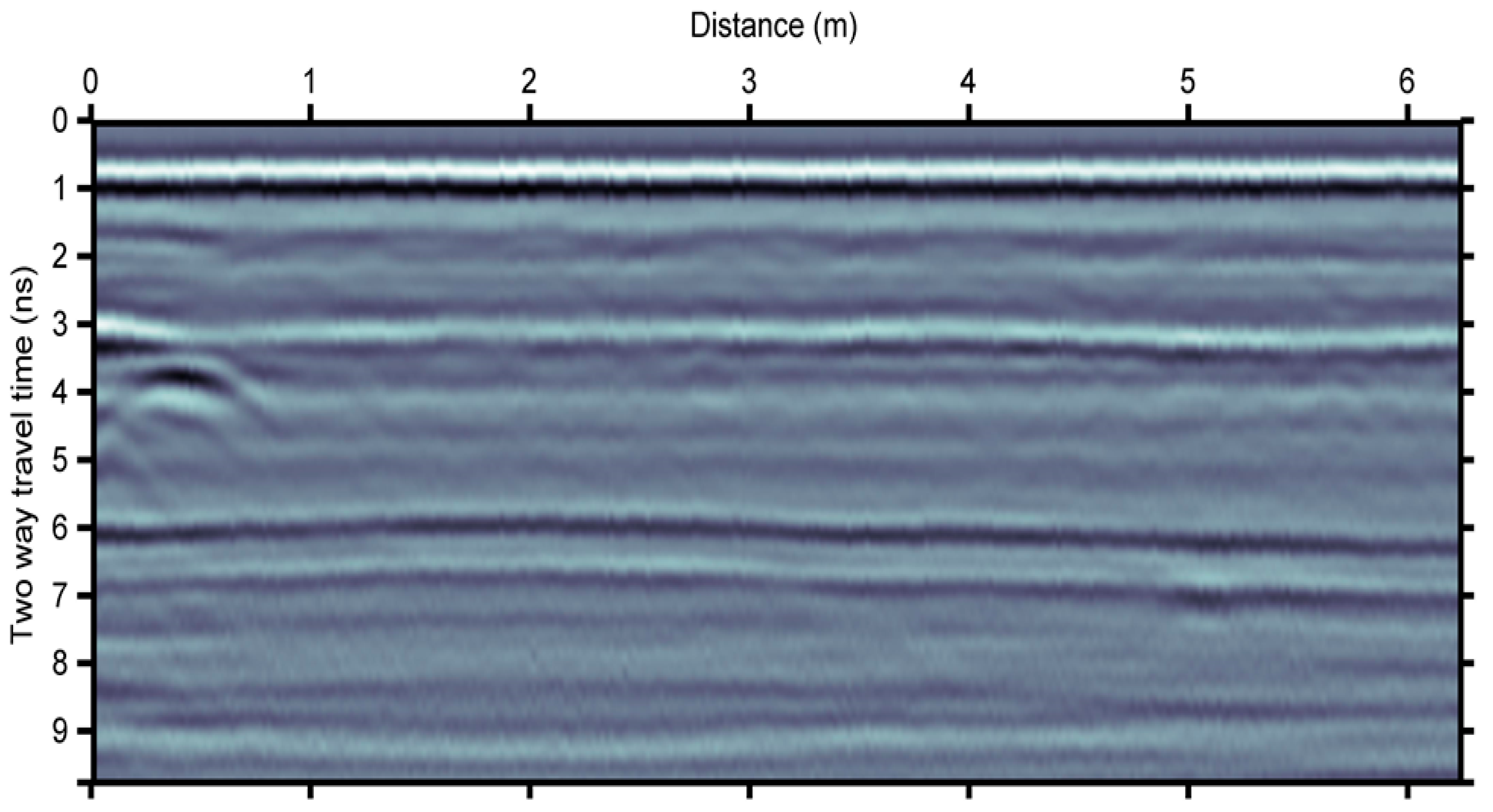
Figure 6 shows the reference GPR radargram after applying a de-wow filter. This operation consists in the application of a zero-phase high-pass filter having a cutoff frequency at approximately 2% of the Nyquist frequency of the traces. It is possible to observe that low frequency harmonics are suppressed, especially for arrivals later than 4 ns. This occurrence is particularly evident by comparing Figure 5 and Figure 6.
4.3. Removal of Antenna Ringing
Antenna ringing produces nearly perfect horizontal reflections that might interfere or cover actual reflections and return unreliable outputs. These horizontal-like reflections can also be due by the interaction between antenna and electricity cables, mobile phones, etc. This occurrence is generally referred to as a “background noise” [28].
To suppress this noise from the records, an average GPR trace is calculated using all the traces in the GPR section. The average trace is therefore subtracted to every single GPR trace, sample by sample.
Background noise removal filter can highly modify the layout of a raw GPR trace and it can generally improve the effectiveness of GPR imaging. In addition, as lower frequency harmonics sometimes appear as horizontal-like reflections, this filter may partially act as a de-wow filter.
Nevertheless, it is important for a user to be fully aware of the following two major issues that may arise from its application:
- Part of the significant reflections may be removed. As horizontal-like reflections return amplitude peaks at the same arrival time, these are expected to be cut off once an average trace is subtracted to the entire radargram. This is a critical issue when pavement layering is the target of the investigation.
- Artifacts might be introduced by removing antenna ringing in homogeneous non-reflecting areas, as an average value is subtracted from amplitude values close to zero.
In view of the above, special attention is recommended when using this processing algorithm in road investigations. Specifically, successful applications are reported for the assessment of point reflectors, such as underground utilities and pipes or pavement defects. On the contrary, use of background noise removal is not recommended in pavement structural detailing.
4.4. Signal Gain
Geometrical spreading refers to the amplitude losses at a three-dimensional level and is regarded as independent from frequency. Frequency-dependent attenuation mainly attenuates the higher frequency harmonics more than the lower ones. It is a combination of instinct (based on the physical properties of the media) attenuation and scattering (high grade of heterogeneity). The dispersive EM nature of materials in road pavement layers and subgrade soils causes frequency-dependent attenuation of the propagating EM waves. The rate of dispersion is mostly related to the electrical conductivity of the travelled medium [28]. All of the above features contribute to the high attenuation of an EM signal with time.
Signal gain is generally referred to as a time-varying enhancement of signal amplitudes. It is applied to recover part of the losses caused by attenuation, regardless of the specific mechanism (e.g., absorption and spherical divergence).
According to the above, gain functions involve serious modifications to the recordings that might cause potential data misinterpretations. To this effect, all the components of late arrivals, including noise contributions, are amplified and artifacts might be potentially introduced. This processing algorithm is therefore more effective if applied to data cleared from external noise.
In general, it is worth to remember that signal gain is used only for visual and interpretation purposes and, hence, it requires to be used at the final stage of processing.
Five of the most commonly used gain functions are listed below:
- Automatic Gain Control (AGC). This is an automatic function that is applied to each trace of a GPR section. It is based on the difference between the average amplitude of a signal in a specific time window and the maximum amplitude of the overall trace [62]. A careful selection of the time-window is then crucial to avoid excessive noise or flat areas in the section [63].
- Spreading Exponential Compensation (SEC). This algorithm works automatically on the signal compensating the loss of energy by geometric spreading effects of the travelling wavefront [60]. A drawback of using SEC (sometimes named as Inverse Power Decay filter) is related to an incorrect selection of the exponential gain factor. To this effect, earlier time amplitudes are likely to be hidden by later time amplitudes due to amplification effects.
- Inverse Amplitude Decay (IAD). This is a data adaptive filter that calculates a main amplitude decay function for the whole GPR section. The inverse function is then applied to each trace. In this regard, lateral amplitude variation is maintained and amplitudes in a trace are more enhanced.
- User Defined Gain (UDG), Linear Gain, and Exponential Gain. These algorithms are based on functions with specific mathematical expressions. Most diffused algorithms apply a linear or exponential amplification of the signal in depth, although more complex expressions can be adopted at discretion of the user. Precaution is mostly recommended when using UDG, especially if the user is not experienced.
Regarding the GPR dataset considered in this study, an exponential gain was applied based on the Inverse Amplitude Decay (IAD) method. This method, in the way it is applied in this paper, calculates the Hilbert Transform of each GPR trace and estimates the mean instantaneous amplitude trace (or envelope) of all traces. An exponential function is then fitted through the average envelope trace (Figure 7).
4.5. Band-Pass Filtering
Noise due to the surrounding media and the inherent loss of the GPR signal usually lowers the SNR in a GPR section, especially at relatively late recording times [58,64]. These noise components are generally located outside the main working frequency bandwidth of a GPR system. Bandwidth refers here to the band of frequencies occupied by the central lobe of the spectrum of an electromagnetic signal. Band-pass filter works by cutting off these edge bands from the frequency spectra of the GPR data [65]. In practical terms, this filter is composed of two filters, namely the high-pass and the low-pass. These two algorithms can modify a GPR signal by removing the low- and high-frequency components of the spectrum, respectively, with reference to two fixed thresholds. As an example, an antenna transmitting an EM pulse with a peak frequency of 900 MHz in the frequency domain may have an effective bandwidth from 450 to 1350 MHz. In view of this, frequency harmonics having lower or higher dominant frequencies may need to be cut off.
It is also worthy of mention that noise exists at all recording times, although it is often not visible. It can affect processing such as spectral whitening. The most common reason for applying band-pass filtering is to remove high-frequency random noise, mostly to improve visual quality of data.
Application of band-pass filter algorithms is generally highly effective on GPR data collected in road inspections. High-pass filters work on the noise generated by typical surrounding objects (e.g., vehicles, building, and traffic barriers), whereas low-pass filters cut off signal components generated by EM devices such as mobile phones [66,67].
For the application of stationary band-pass filtering (i.e., having the same cut-off frequency for all the recording times and traces), it is advisable that the band stop (or band-pass) frequency values are identified with care after a comprehensive analysis of several representative traces. If applicable, the most correct approach is to apply time-varying band-pass filtering. For example, EMD [58] or a user-defined time varying band-pass filtering in the t-f domain [64] could be used.
In general, there is no unique rule in setting thresholds for low- and high-pass filters. An analysis of the collected signal in the frequency domain should help with the choice, case by case. An inaccurate setting of the filter bandwidth causes a non-optimal filtering of the noise or, most likely, a loss of relevant information contained in the removed frequency bands [63]. As a rule of thumb, a bandwidth of 1.5 times the central frequency of investigation can be preliminarily used [6,63].
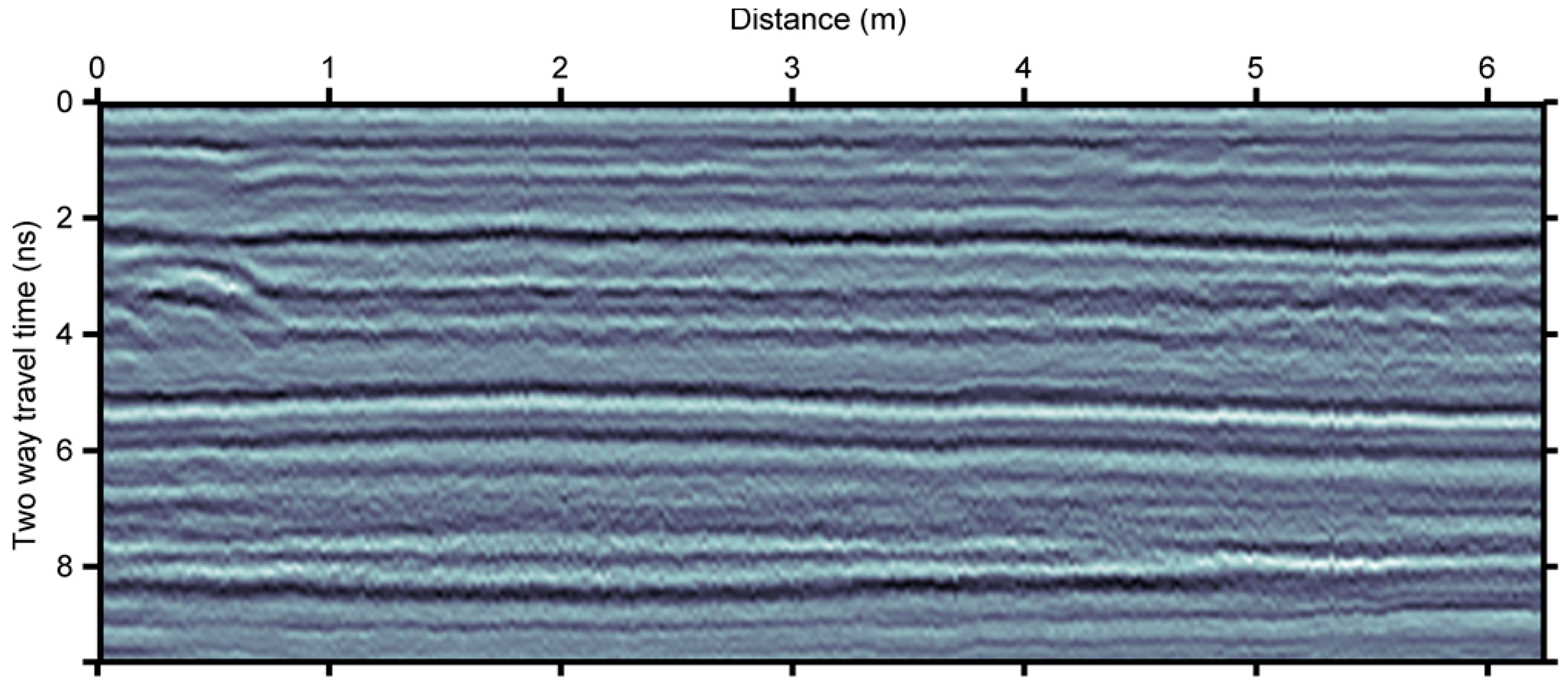
Analysis of the GPR section in Figure 8 indicates relatively low-frequency harmonics (i.e., the reflection at around 4 ns, white color) and relatively higher frequency harmonics attributed to random noise, especially after around 6.5 ns. A band-pass filter (selected frequency band 618 –MHz) was applied on the data depicted in Figure 6 followed by an IAD gain (Figure 9). Comparison of sections in Figure 8 and Figure 9 shows the suppression of unwanted harmonics after band-pass filtering. Blurring due to lower frequency harmonics and higher frequency noise are both not present.
4.6. Special Processing Steps
4.6.1. Vertical or Time Resolution Enhancement
Vertical resolution is generally referred to as the smallest size of an object that it is possible to detect with a given GPR system. This depends mainly on both the features of a GPR system (e.g., the central frequency) and the dielectric properties of the investigated medium [68]. Practically, enhancement of temporal resolution is aimed to reduce the pulse width of the GPR data (i.e., to squeeze the dominant wavelets in time). This is mostly achieved through statistical deconvolution methods such as spiking and predictive (if a small lag is utilized) deconvolution is often used in seismic analyses.
However, statistical methods are usually not robust for application to GPR traces, due to the significant non-stationarity of the signal. The most important factor of non-stationarity is the time-varying dominant frequency value decrease with increasing recording time. This requires a time-gated (or a time-varying) deconvolution approach.
Thereby, deterministic deconvolution represents a more straightforward approach for GPR applications. In this method, a reference wavelet is required [69,70]. For air-coupled antenna systems, an acquisition carried out over a metal plate is an adequate reference. In the case of ground-coupled GPR systems, a reflection from a metal plate may not produce a satisfactory output, making this method less applicable. Most commercial software tools nowadays do not involve time-varying deconvolution. In this paper the method described in [70] is used. Time-varying spectral shaping is first performed in the t-f domain over time windows of 2 ns duration, followed by an inverse filtering based on the amplitude spectrum of a reflection from a metal plate (Figure 10).
Shallow layers in flexible pavements are mainly made of HMA materials and their thickness ranges between 3 and 10 cm. Therefore, these layers are beyond the vertical resolution of the systems that are most likely used for road inspections (1000–2000 MHz of central frequency). Hence, it is not rare that reflections from the top and the bottom of these particular layers may overlap, thereby not allowing for thickness estimation. Accordingly, vertical resolution enhancement stands as a crucial processing step for specialist applications such as QC/QA and HMA density assessment.
In Figure 10, the GPR section represented in Figure 9 is depicted after time-varying deconvolution. It is possible to notice an additional reflection in dark color at around 0.86 ns from the wearing/binder interface, that was not detectable before the application of the deconvolution processing step.
4.6.2. Migration or Lateral Resolution Enhancement
This processing method stands as a spatial deconvolution [71] for reconstruction of the main geometric features of reflecting objects. This is performed by correcting the radar reflectivity in the subsurface and it mainly increases the lateral resolution. This type of processing requires knowledge of the traveling wave velocity model [63].
Overall, migration has two major effects, namely, locating reflectors at their correct position and gathering energy of diffractions. The user must consider that, theoretically, diffractions after migration disappear and the GPR section eventually consists only of reflections located at their correct position.
4.6.3. Time-to-Depth Conversion
GPR time sections can be converted to depth sections using a velocity model. This is particularly useful in road inspections, as it allows an estimation of the thicknesses of pavement layers as well as to locate the actual depth of decays. As a detailed velocity model is rarely determined in road applications, a constant average value of propagation velocity is generally assigned to each layer. This velocity value is estimated from the cores extracted on the pavement [6]. In this case, accuracy of depth conversion depends on the number of cores and their spacing, as the velocity is interpolated. Main drawbacks of this technique are the invasiveness of the core extraction and a relatively low representativeness of the actual conditions, especially when number of cores is very limited.
Among the self-reliant methods for estimation of the propagation velocity from GPR only, the “common midpoint” (CMP) and the “hyperbolic velocity analysis” are worthy of mention.
The former is applied by collecting data with a bi-static GPR system, at different positions of the transmitting and the receiving antennas. In more detail, antennas are progressively moved apart such that a common midpoint is fixed at the same abscissa. It is possible to estimate the propagation velocity by way of comparison between the various acquisitions as well as by geometrical assumptions [72]. An alternative to this technique is to acquire common-source and multi-receiver data and further rearrange this information in CMPs for velocity analysis.
On the other hand, the hyperbolic velocity analysis is based on the analysis of diffractions within a relevant section. The slope of the hyperbola branches depends on the best migration velocity (i.e., the velocity that best suits the diffraction), which in turn is a function of the propagation velocity. Hence, it relates also to the dielectric constant of the specific material.
Both methods have drawbacks in the processing of road datasets. The CMP method requires use of a bi-static GPR system, which is not suitable for air-coupled investigations, although an extended version of the method (XCMP) using two air-coupled GPR systems has been recently proposed [73]. In addition, as current technology is moving towards use of multi-channel GPR systems, this appears as a promising method for future improvements. Conversely, a hyperbolic velocity analysis requires frequent clear diffractions in each layer to estimate the tendency of the propagation velocity. This is unlikely to verify in quasi-homogeneous multi-layered media such as the layers of a road pavement.
Application of migration and time-to-depth conversion to the GPR section in Figure 10 (using the velocity information in Table 4) produces the GPR depth section shown in Figure 11. Note that the reflection at the bottom of the first layer clearly indicates a first layer with a thickness of around 0.06 m and a second layer with a thickness of around 0.10 m.
The ground-truth information at the base of the time-to-depth conversion is reported in Table 4. In this paper, we consider that interval velocity is constant within each layer for the whole GPR section. However, there is ambiguity between layer thickness variation and interval velocity variation, as already discussed in the first paragraph of this section. This raises the need for more laterally accurate velocity estimation.
5. Discussion
In this work, a signal processing procedure for GPR data collected in road inspections is introduced to cover the widest possible range of users’ expertise. The main aim is to discuss well-established and most advanced processing steps as a unique processing flow.
However, it is worth to mention that data processing is a user-defined process. Outputs are always affected by user-defined parameters set during the processing stage. In this regard, data adaptive algorithms should be implemented to reduce this ambiguity and increase the automation [74].
In addition, it is expected for data processing to fail when an attempt is made at providing satisfactory results for all the types of data. This mainly depends on the extremely complex and variable nature of the subsurface, which causes EM energy scattering. Scattering, in addition to causing low SNR values, is one of the causes for decreased Q* values, which also alter the shape of the waveforms and increase the non-stationarity of the GPR traces [64]. Clay content (bounded water) and free water are also factors that decrease Q* values and increase conductivity, with the latter being dominant for the dependency of the signal total amplitude. When the SNR is low, the effectiveness of almost all the processing methods decreases as well. However, a low SNR is not only dependent on the subsurface, but also on the acquisition process. The use of a suitable antenna system and dense measurements may improve SNR at some extent and lower the risk to produce unsatisfactory results or misinterpretations of the outcomes during the data processing implementation.
Nowadays, most common processing steps in road monitoring applications include the de-wow filtering, the background noise removal filtering, the band-pass filtering, the time-varying trace-to-trace gain and the time-to-depth conversion. It is worth to mention that the latter step is not used in all the cases. The most advanced processing methods presented in this paper, such as deconvolution and migration, have been a matter of research for many years, especially in seismics. New methods are introduced every year with applicability to different subsurface conditions. However, these methods are most likely not to work in comparison to conventional methods, especially under varying subsurface conditions. This is mostly due to the instability of inverse filtering or other numerical problems such as the large number of user-defined parameters required. As an example, time windowing for time-varying deconvolution, which is essential to deal with non-stationarity, is a user-defined parameter that can be used based on the amplitude or dominant frequency variation. The choice of a pre-whitening value for stable inverse filtering is also a user-defined parameter, which is heavily dependent on the data. Both of the above are a matter of research nowadays and proposed solutions are not always successful in terms of results. Moreover, a lack of expertise among the GPR community (which is large in the seismic industry) in this specific type of processing implies that advanced processing methods are rarely used, leading to a relatively frequent data misinterpretation. In view of this, future research could task itself in fostering automation for the application of these methods.
In regard to the need of an accurate EM velocity model, multi-channel GPR systems nowadays allow for both an evaluation of a velocity model and a detailed analysis of its change in depth, with an additional estimation of the moisture variation. The main issue is the large volume of data requiring an advanced processing by qualified operators, as it happens nowadays in seismic reflection data analysis. A good strategy to deal with this volume of data is to perform a velocity analysis at sparse arrays along the road and further to focus on areas of interest. Nevertheless, the volume of data remains large when dealing with distances of kilometers sampled at a centimeter resolution. To overcome this issue, full-waveform inversion can be used, although this arises pre-processing and heavy computational issues along with the accuracy of the initial velocity model [75].
6. Conclusions
This study reports a signal processing method for ground penetrating radar (GPR) data collected on flexible pavements. Working principles of GPR as well as main survey configurations used in road inspections are discussed. A multi-stage method is presented and results are shown against data collected on a real-life flexible pavement structure. To this effect, main considerations about the effects of each step are given by way of comparison between processed and unprocessed radargrams. Stages of the method include: (i) raw signal correction; (ii) removal of lower frequency harmonics; (iii) removal of antenna ringing; (iv) band-pass filtering; and (v) signal gain. Use of special processing steps such as vertical resolution enhancement, migration and time-to-depth conversion are finally discussed.
Efficient migration and time-to-depth conversion require an as detailed as possible velocity model. This emphasizes the need for using multi-channel radar systems, which are expected to be increasingly employed in road inspections in view of the hardware technological advances. Future research could focus on the use of multi-channel GPR data processing, in regard to the automation and the time consumption of the involved techniques for velocity analysis. In addition, an increased data adaptiveness across all the processing steps could pave the way to a more comprehensive and effective interpretation of the GPR sections.
Author Contributions
Conceptualization, L.B.C. and F.T.; Methodology, F.B. and N.E.; Software, F.B. and N.E.; Validation, N.E. and F.B.; Formal Analysis, F.T. and L.B.C.; Investigation, F.T. and L.B.C.; Resources, F.B.; Data Curation, N.E.; Writing—Original Draft Preparation, L.B.C. and N.E.; Writing—Review & Editing, F.T. and N.E.; Visualization, L.B.C.; Supervision, F.B.
Funding
This research received no external funding.
Acknowledgments
The authors express their gratitude to IDS Georadar S.p.A. for providing part of the GPR equipment used in the experimental activities.
Conflicts of Interest
The authors declare no conflict of interest.
References
- World Health Organisation. Global Status Report on Road Safety 2015; World Health Organisation: Geneve, Switzerland, 2015. [Google Scholar]
- European Commission. Towards a European Road Safety Area: Policy Orientations on Road Safety 2011–2020; COM(2010) 389, 2010; The European Automotive Manufacturers Association: Brussels, Belgium, 2010. [Google Scholar]
- Tighe, S.; Li, N.; Falls, L.C.; Haas, R. Incorporating road safety into pavement management. Transport. Res. Rec. 2000, 1699, 1–10. [Google Scholar] [CrossRef]
- Beskou, N.D.; Theodorakopoulos, D.D. Dynamic effects of moving loads on road pavements: A review. S. Dyn. Earthq. Eng. 2011, 31, 547–567. [Google Scholar] [CrossRef]
- D’Amico, F.; Calvi, A.; Bianchini Ciampoli, L.; Tosti, F.; Brancadoro, M.G. Evaluation of the impact of pavement degradation on driving comfort and safety using a dynamic simulation model. Adv. Transport. Stud. 2018, 1, 109–120. [Google Scholar] [CrossRef]
- Benedetto, A.; Tosti, F.; Bianchini Ciampoli, L.; D’Amico, F. An overview of ground-penetrating radar signal processing techniques for road inspections. Signal Process. 2017, 132, 201–209. [Google Scholar] [CrossRef] [Green Version]
- Marecos, V.; Fontul, S.; Antunes, M.L.; Solla, M. Evaluation of a highway pavement using non-destructive tests: Falling Weight Deflectometer and Ground Penetrating Radar. Constr. Build. Mater. 2017, 151, 1164–1172. [Google Scholar] [CrossRef]
- Frangopol, D.M.; Liu, M. Maintenance and management of civil infrastructure based on condition, safety, optimization, and life-cycle cost. Struct. Infrastruct. Eng. 2007, 1, 29–41. [Google Scholar] [CrossRef]
- Sheils, E.; O’Connor, A.; Breysse, D.; Schoefs, F.; Yotte, S. Development of a two-stage inspection process for the assessment of deteriorating infrastructure. Reliab. Eng. Syst. Saf. 2010, 1, 29–41. [Google Scholar] [CrossRef]
- Capozzoli, L.; Rizzo, E. Combined NDT techniques in civil engineering applications: Laboratory and real test. Constr. Build. Mater. 2017, 154, 1139–1150. [Google Scholar] [CrossRef]
- Sebaaly, B.E.; Mamlouk, M.S.; Davies, T.G. Dynamic analysis of falling weight deflectometer data. Transport. Res. Rec. 1986, 1070, 63–68. [Google Scholar]
- Rohde, G.T. Determining pavement structural number from FWD testing. Transport. Res. Rec. 1994, 1448, 61–68. [Google Scholar]
- Mehta, Y.; Roque, R. Evaluation of FWD data for determination of layer moduli of pavements. J. Mater. Civ. Eng. 2003, 15, 25–31. [Google Scholar] [CrossRef]
- Cosenza, P.; Marmet, E.; Rejiba, F.; Jun, C.Y.; Tabbagh, A.; Charlery, Y. Correlations between geotechnical and electrical data: A case study at Garchy in France. J. Appl. Geophys. 2006, 60, 165–178. [Google Scholar] [CrossRef]
- Maślakowski, M.; Kowalczyk, S.; Mieszkowski, R.; Józefiak, K. Using electrical resistivity tomography (ERT) as a tool in geotechnical investigation of the substrate of a highway. Stud. Quat. 2014, 31, 83–89. [Google Scholar] [CrossRef]
- Saarenketo, T.; Scullion, T. Road evaluation with ground penetrating radar. In Proceedings of the 7th International Conference on Ground-Penetrating Radar (GPR98), Lawrence, KS, USA, 27–30 May 1998. [Google Scholar] [CrossRef]
- Benedetto, A.; Pensa, S. Indirect diagnosis of pavement structural damages using surface GPR reflection techniques. J. Appl. Geophys. 2007, 62, 107–123. [Google Scholar] [CrossRef]
- Loizos, A.; Plati, C. Accuracy of ground penetrating radar horn-antenna technique for sensing pavement subsurface. IEEE Sens. J. 2007, 7, 842–850. [Google Scholar] [CrossRef]
- Lahouar, S.; Al-Qadi, I.L. Automatic detection of multiple pavement layers from GPR data. Non-Destr. Test. Eval. Int. 2008, 41, 69–81. [Google Scholar] [CrossRef]
- Fernandes, F.M.; Fernandes, A.; Pais, J. Assessment of the density and moisture content of asphalt mixtures of road pavements. Constr. Build. Mater. 2017, 154, 1216–1225. [Google Scholar] [CrossRef]
- Liu, H.; Sato, M. In situ measurement of pavement thickness and dielectric permittivity by GPR using an antenna array. Non-Destr. Test. Eval. Int. 2014, 64, 65–71. [Google Scholar] [CrossRef]
- Tosti, F.; Bianchini, C.L.; D’Amico, F.; Alani, A.M.; Benedetto, A. An experimental-based model for the assessment of the mechanical properties of road pavements using ground-penetrating radar. Constr. Build. Mater. 2018, 165, 966–974. [Google Scholar] [CrossRef]
- Maser, K.R.; Roddis, W.M.K. Principles of thermography and radar for bridge deck assessment. J. Transp. Eng. 1990, 116, 583–601. [Google Scholar] [CrossRef]
- Mothé, M.G.; Leite, L.F.M.; Mothé, C.G. Thermal characterization of asphalt mixtures by TG/DTG, DTA and FTIR. J. Therm. Anal. Calorim. 2008, 93, 105–109. [Google Scholar] [CrossRef]
- Solla, M.; Lagüela, S.; González-Jorge, H.; Arias, P. Approach to identify cracking in asphalt pavement using GPR and infrared thermographic methods: Preliminary findings. Non-Destr. Test. Eval. Int. 2014, 62, 55–65. [Google Scholar] [CrossRef]
- Chang, K.T.; Chang, J.R.; Liu, J.K. Detection of pavement distresses using 3D laser scanning technology. In Proceedings of the 2005 ASCE International Conference on Computing in Civil Engineering, Cancun, Mexico, 12–15 July 2005; pp. 1085–1095. [Google Scholar]
- Guan, H.; Li, J.; Cao, S.; Yu, Y. Use of mobile LiDAR in road information inventory: A review. Int. J. Image Data Fusion 2016, 7, 219–242. [Google Scholar] [CrossRef]
- Daniel, D.J. Ground Penetrating Radar, 2nd ed.; The Institution of Electrical Engineers: London, UK, 2004. [Google Scholar]
- Slob, E.C.; Sato, M.; Olhoeft, G. Surface and borehole ground-penetrating-radar developments. Geophysics 2010, 75, 75A103–75A120. [Google Scholar] [CrossRef]
- Benedetto, F.; Tosti, F.; Alani, A.M. An entropy-based analysis of GPR data for the assessment of railway ballast conditions. IEEE Trans. Geosci. Remote Sens. 2017, 55, 3900–3908. [Google Scholar] [CrossRef]
- Al-Qadi, I.L.; Lahouar, S. Measuring layer thicknesses with GPR - Theory to practice. Constr. Build. Mater. 2005, 19, 763–772. [Google Scholar] [CrossRef]
- Bastard, C.L.; Baltazart, V.; Wang, Y.; Saillard, J. Thin-pavement thickness estimation using GPR with high-resolution and superresolution methods. IEEE Trans. Geosci. Remote Sens. 2007, 45, 2511–2519. [Google Scholar] [CrossRef]
- Loizos, A.; Plati, C. Accuracy of pavement thicknesses estimation using different ground penetrating radar analysis approaches. Non-Destr. Test. Eval. Int. 2014, 62, 55–65. [Google Scholar] [CrossRef]
- Maser, K.R. Condition assessment of transportation infrastructure using ground-penetrating radar. J. Infr. Syst. 1996, 43, 119–138. [Google Scholar] [CrossRef]
- Al-Qadi, I.L.; Lahouar, S.; Loulizi, A. In situ measurements of hot-mix asphalt dielectric properties. Non-Destr. Test. Eval. Int. 2001, 34, 427–434. [Google Scholar] [CrossRef]
- Chen, D.H.; Scullion, T. Forensic investigations of roadway pavement failures. J. Perform. Constr. Facil. 2008, 22, 35–44. [Google Scholar] [CrossRef]
- Saarenketo, T. Electrical properties of water in clay and silty soils. J. Appl. Geophys. 1998, 40, 73–88. [Google Scholar] [CrossRef]
- Benedetto, A. Water content evaluation in unsaturated soil using GPR signal analysis in the frequency domain. J. Appl. Geophys. 2010, 71, 26–35. [Google Scholar] [CrossRef]
- Tosti, F.; Benedetto, A.; Bianchini Ciampoli, L.; Lambot, S.; Patriarca, C.; Slob, E.C. GPR analysis of clayey soil behaviour in unsaturated conditions for pavement engineering and geoscience applications. Near Surf. Geophys. 2016, 14, 127–144. [Google Scholar] [CrossRef]
- Dérobert, X.; Iaquinta, J.; Klysz, G.; Balayssac, J.-P. Use of capacitive and GPR techniques for the non-destructive evaluation of cover concrete. Non-Destr. Test. Eval. Int. 2008, 62, 55–65. [Google Scholar] [CrossRef]
- Alani, A.M.; Aboutalebi, M.; Kilic, G. Applications of ground penetrating radar (GPR) in bridge deck monitoring and assessment. J. App. Geophys. 2013, 97, 45–54. [Google Scholar] [CrossRef]
- Diamanti, N.; Annan, A.P.; Redman, J.D. Concrete Bridge Deck Deterioration Assessment Using Ground Penetrating Radar (GPR). J. Environ. Eng. Geophys. 2017, 22, 121–132. [Google Scholar] [CrossRef]
- Benedetto, F.; Tosti, F. A signal processing methodology for assessing the performance of ASTM standard test methods for GPR systems. Signal Process. 2017, 132, 327–337. [Google Scholar] [CrossRef] [Green Version]
- ASTM International. ASTM D6087-08(2015)e1, Standard Test Method for Evaluating Asphalt-Covered Concrete Bridge Decks Using Ground Penetrating Radar. Available online: https://www.astm.org/Standards/D6087.htm (accessed on 10 December 2018).
- Saarenketo, T. NDT Transportation. In Ground Penetrating Radar; Elsevier: Amsterdam, The Netherlands, 2009; pp. 393–444. [Google Scholar]
- Golgowski, G. Arbeitsanleitung fur den Einsatz des Georadarszur Gewinnung von Bestandsdaten des Fahrbahnaufbaues; AbteilungStraßenbautechnik: Berlin, Germany, 2003. [Google Scholar]
- Sebesta, S.; Scullion, T. Using Infrared Imaging and Ground-Penetrating Radar to Detect Segregation in Hot-Mix Asphalt Overlays; Research Report 4126-1; Texas Department of Transportation, Texas A&M University: College Station, TX, USA, 2002. [Google Scholar]
- Clark, M.R.; Gillespie, R.; Kemp, T.; McCann, D.M.; Forde, M.C. Electromagnetic properties of railway ballast. Non-Destr. Test. Eval. Int. 2004, 34, 305–311. [Google Scholar] [CrossRef]
- Puente, I.; Solla, M.; González-Jorge, H.; Arias, P. NDT documentation and evaluation of the roman bridge of lugo using GPR and mobile and static LiDAR. J. Perform. Constr. Facil. 2015, 29. [Google Scholar] [CrossRef]
- Annan, A.P. Practical processing of GPR data. In Proceedings of the EAGE 2001 Conference, Delft, The Netherlands, 11–15 June 2001. [Google Scholar]
- Persico, R. Introduction to Ground Penetrating Radar: Inverse Scattering and Data Processing; Wiley Blackwell: Hoboken, NJ, USA, 2014. [Google Scholar]
- Olhoeft, G.R. Maximizing the information return from ground penetrating radar. J. Appl. Geophys. 2000, 43, 175–187. [Google Scholar] [CrossRef]
- Nobes, D.C. Geophysical surveys of burial sites: A case study of the Oarourupa. Geophysics 1999, 64, 357–367. [Google Scholar] [CrossRef]
- Yelf, R. Where is true time zero? In Proceedings of the Tenth International Conference on Grounds Penetrating Radar GPR 2004, Delft, The Netherlands, 21–24 June 2004. [Google Scholar]
- Davis, J.L.; Annan, A.P. Ground penetrating radar to measure soil water content. In Methods of Soil Analysis, Part 4; Dane, J.H., Topp, G.C., Eds.; Soil Science Society of America (SSSA): Washington, DC, USA, 2002; pp. 446–463. [Google Scholar]
- Dougherty, E.R. Optimal mean-absolute-error filtering of gray-scale signals by the morphological hit-or-miss transform. J. Math. Imaging Vis. 1994, 4, 255–271. [Google Scholar] [CrossRef]
- Gerlitz, K.; Knoll, M.D.; Cross, G.M.; Luzitano, R.D.; Knight, R. Processing ground penetrating radar data to improve resolution of near-surface targets. In Proceedings of the Symposium on the Application of Geophysics to Engineering and Environmental Problems, San Diego, CA, USA, 18–22April 1993. [Google Scholar]
- Battista, B.M.; Addison, A.D.; Knapp, C.C. Empirical Mode Decomposition Operator for Dewowing GPR Data. J. Environ. Eng. Geophys. 2009, 14, 163–169. [Google Scholar] [CrossRef] [Green Version]
- Lambot, S.; Slob, E.C.; Van Bosch, I.D.; Stockbroeckx, B.; Vanclooster, M. Modeling of ground-penetrating radar for accurate characterization of subsurface electric properties. IEEE Trans. Geosci. Remote Sens. 2004, 42, 2555–2568. [Google Scholar] [CrossRef]
- Soldovieri, F.; Lopera, O.; Lambot, S. Combination of advanced inversion techniques for an accurate target localization via GPR for demining applications. IEEE Trans. Geosci. Remote Sens. 2011, 49, 451–461. [Google Scholar] [CrossRef]
- De Coster, A.; Lambot, S. Full-Wave Removal of Internal Antenna Effects and Antenna-Medium Interactions for Improved Ground-Penetrating Radar Imaging. IEEE Trans. Geosci. Remote Sens. 2019, 57, 93–103. [Google Scholar] [CrossRef]
- Jol, H. Ground Penetrating Radar: Theory and Applications; Elsevier: Amsterdam, The Netherlands, 2009. [Google Scholar]
- Horstmeyer, H.; Gurtner, M.; Buker, F.; Green, A. Processing 2-D and 3-D georadar data: Some special requirements. In Proceedings of the Second Meeting of the Environmental and Engineering Geophysical Society, European section, Nantes, France, 2–5 September 1996. [Google Scholar]
- Economou, N.; Vafidis, A. Spectral balancing GPR data using time-variant bandwidth in the t-f domain. Geophysics 2010, 75, J19–J27. [Google Scholar] [CrossRef]
- Sun, J.; Young, R.A. Recognizing surface scattering in ground-penetrating radar data. Geophysics 1995, 60, 1378–1385. [Google Scholar] [CrossRef]
- Bano, M.; Pivot, F.; Methelot, J.M. Modelling and Filtering of Surface Scattering in Ground-penetrating Radar Waves. First Break 1999, 17, 215–222. [Google Scholar] [CrossRef]
- Nuzzo, L. Coherent noise attenuation in GPR data linear and parabolic radon transform techniques. Ann. Geophys. 2003, 46, 533–547. [Google Scholar] [CrossRef]
- Spagnolini, U. Permittivity measurements of multi layered media with monostatic pulse radar. IEEE Trans. Geosci. Remote Sens. 1997, 35, 454–463. [Google Scholar] [CrossRef]
- Chahine, K.; Vincent, B.; Wang, Y.; Dérobert, X. Blind deconvolution via sparsity maximization applied to GPR data. Eur. J. Environ. Civ. Eng. 2011, 15, 575–586. [Google Scholar] [CrossRef]
- Economou, N.; Vafidis, A. Deterministic deconvolution for GPR data in t-f domain. Near Surf. Geophys. 2011, 9, 427–433. [Google Scholar] [CrossRef]
- Fisher, E.; McMechan, G.A.; Annan, A.P.; Cosway, S.W. Examples of reverse-time migration of single-channel, ground-penetrating radar profiles. Geophysics 1992, 57, 577–586. [Google Scholar] [CrossRef]
- Tillard, S.; Dubois, J.C. Influence and lithology on radar echoes: Analysis with respect to electromagnetic parameters and rock anisotropy. Spec. Paper—Geol. Surv. Finl. 1992, 16, 95–102. [Google Scholar]
- Zhao, S.; Al-Qadi, I.L. Super-Resolution of 3-D GPR Signals to Estimate Thin Asphalt Overlay Thickness Using the XCMP Method. IEEE Trans. Geosci. Remote Sens. 2018. in Press. [Google Scholar] [CrossRef]
- Economou, N. Time varying band pass filtering GPR data by self- inverse filtering. Near Surf. Geophys. 2016, 14, 207–217. [Google Scholar]
- Lavoué, F.; Brossier, R.; Métivier, L.; Garambois, S.; Virieux, J. Two-dimensional permittivity and conductivity imaging by full waveform inversion of multioffset GPR data: A frequency-domain quasi-Newton approach. Geophys. J. Int. 2014, 197, 248–268. [Google Scholar] [CrossRef]
Figure 1.
General layout of a GPR system.

Figure 2.
A typical GPR system configuration used for road inspections.

Figure 3.
Raw GPR data collected by the HI-Pave HR system, manufactured by IDS S.p.A., equipped with an air-coupled antenna.
Figure 3.
Raw GPR data collected by the HI-Pave HR system, manufactured by IDS S.p.A., equipped with an air-coupled antenna.

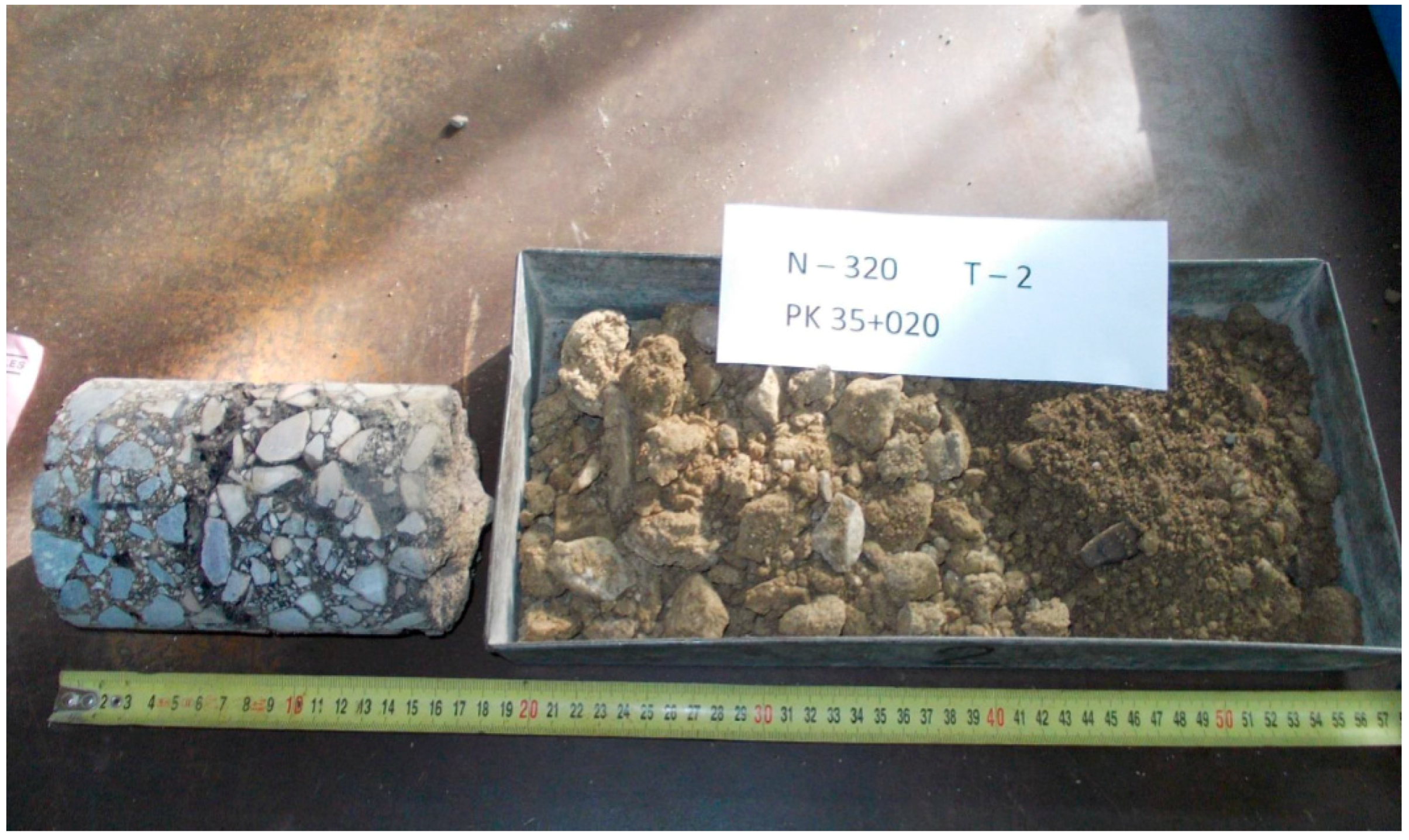
Figure 4.
Pavement structure by a reference sampling core.

Figure 5.
The GPR section after time-zero corrections.

Figure 6.
The GPR section after the application of a de-wow filter.

Figure 7.
The average instantaneous amplitude (or envelope) of all the GPR traces depicted in Figure 6 (continuous line) and an exponential function fitted through it (dashed line).
Figure 7.
The average instantaneous amplitude (or envelope) of all the GPR traces depicted in Figure 6 (continuous line) and an exponential function fitted through it (dashed line).

Figure 8.
The GPR section represented in Figure 6 after the application of the IAD gain.
Figure 8.
The GPR section represented in Figure 6 after the application of the IAD gain.

Figure 9.
The GPR section after the application of a band-pass filter to the section represented in Figure 6 and the application of the IAD gain.
Figure 9.
The GPR section after the application of a band-pass filter to the section represented in Figure 6 and the application of the IAD gain.

Figure 10.
Deconvolved GPR section.

Figure 11.
The GPR section subject to migration and time-to-depth conversion after deconvolution.


Table 1.
Main NDT methods used in road surveys.
| NDT | Acronym | Applications | References |
|---|---|---|---|
| Falling Weight Deflectometer | FWD | pavement stiffness measurement | [11,12,13] |
| Electrical Resistivity Tomography | ERT | presence of voids, moisture assessment | [14,15] |
| Ground Penetrating Radar | GPR | structural detailing, deep defects detection, moisture/clay evaluation | [16,17,18,19,20,21,22] |
| Infrared Thermography | IRT | defects detection, moisture assessment | [23,24,25] |
| Terrestrial Laser Scanner | TLS | surface defects detection | [26,27] |
Table 2.
Main GPR applications in road surveys.
| Application | References |
|---|---|
| Evaluation of layer thicknesses | [31,32,33] |
| Assessment of damage condition in hot-mixed asphalt (HMA) layers, unbound layers and subgrade soils | [34,35,36] |
| Water and clay content assessment | [37,38,39] |
| Inspection of concrete structural elements | [40,41,42] |
Table 3.
The structure of the surveyed pavement.
| Layer | Type of Structure | Thickness (m) |
|---|---|---|
| Wearing | Hot Mix Asphalt (HMA) | 0.06 |
| Binder | HMA | 0.10 |
| Base | Bitumen-bond granular | 0.20 |
| Subbase | Granular | 0.20 |
Table 4.
Interpretation of the GPR depth section depicted in Figure 11.
Table 4.
Interpretation of the GPR depth section depicted in Figure 11.
| Layer | Material | Depth (m) | Picked Time (ns) | Velocity (m/ns) |
|---|---|---|---|---|
| Wearing | HMA | 0.06 | 0.86 | 0.140 |
| Binder | HMA | 0.16 | 2.38 | 0.131 |
| Base | Bitumen-bound granular | 0.36 | 5.53 | 0.127 |
| Subbase | Loose granular | 0.56 | 7.83 | 0.174 |
© 2019 by the authors. Licensee MDPI, Basel, Switzerland. This article is an open access article distributed under the terms and conditions of the Creative Commons Attribution (CC BY) license (http://creativecommons.org/licenses/by/4.0/).
Share and Cite
MDPI and ACS Style
Bianchini Ciampoli, L.; Tosti, F.; Economou, N.; Benedetto, F. Signal Processing of GPR Data for Road Surveys. Geosciences 2019, 9, 96. https://doi.org/10.3390/geosciences9020096
AMA Style
Bianchini Ciampoli L, Tosti F, Economou N, Benedetto F. Signal Processing of GPR Data for Road Surveys. Geosciences. 2019; 9(2):96. https://doi.org/10.3390/geosciences9020096
Chicago/Turabian StyleBianchini Ciampoli, Luca, Fabio Tosti, Nikos Economou, and Francesco Benedetto. 2019. "Signal Processing of GPR Data for Road Surveys" Geosciences 9, no. 2: 96. https://doi.org/10.3390/geosciences9020096
Note that from the first issue of 2016, this journal uses article numbers instead of page numbers. See further details here.