Testing Market Efficiency with Nonlinear Methods: Evidence from Borsa Istanbul


Finance Department, Baku Engineering University, Baku AZ0101, Azerbaijan
Int. J. Financial Stud. 2019, 7(2), 27; https://doi.org/10.3390/ijfs7020027
Submission received: 21 March 2019
/
Revised: 10 May 2019
/
Accepted: 13 May 2019
/
Published: 4 June 2019
Abstract
:Market efficiency has been analyzed through many studies using different linear methods. However, studies on financial econometrics reveal that financial time series exhibit nonlinear patterns because of various reasons. This paper examines market efficiency at Borsa Istanbul using a smooth transition autoregressive (STAR) type nonlinear model. I develop nonlinear ARCH and STAR models, a linear AR model and random walk model for 10 years’ weekly data and then out-of-sample forecast next 12 weeks’ return. Comparing forecast performance powers, I find that the STAR model outperforms random walk, that is Borsa Istanbul returns are predictable at the given period. The results show that the shareholders may earn abnormal return and identify the direction of the return change for the next week with at least 66% accuracy. Contrary to the linear level studies, these findings show that the Borsa Istanbul is not weak form efficient at nonlinear level within the studied period.
JEL Classification:
G14; G10; G171. Introduction
The efficient-market hypothesis is one of the most famous financial concepts since it was developed in the 1970s. Fama (1970) defines efficient market as a market where asset prices reflect all available information. After then, many studies have examined market efficiency using various linear models (see Basu (1977); Jensen (1978); Rosenberg et al. (1985); Busse and Green (2002); Karan and Gonenc (2003); Metghalchi et al. (2018)). However, recent advances in the literature have shown that financial time series exhibit nonlinear dynamics (Franses and van Dijk (2000); Kumar Narayan (2005)). Several studies find market frictions, transaction costs, short selling, arbitrage limits, and other reasons create asymmetrical and nonlinear patterns in financial time series (Hasanov and Omay (2008)). In particular, asset returns exhibit momentum or positive correlation over a short horizon, but negative correlation over a longer horizon, hence those returns are characterized by persistence and slow reversion (Campbell et al. 1997). Linear models are insufficient to capture those dynamics.
That nonlinearity in time series may originate either from conditional mean or conditional variance, or both. If the nonlinearity is simply a result of conditional variance, such series are modeled through autoregressive conditional heteroscedasticity (ARCH) models developed by Engle (1982). Nonlinear time series of conditional mean are modeled with threshold autoregressive models (TAR) or Markov switching models. The TAR models assume that the regimes can be determined by observable variables xt. These models can be expressed by the equation
where ϕj(xt) (j = 0, 1, ..., p) is a parametric function of xt variable.
Markov switching models assume that the regimes are not exactly observed, however they are defined with the non-observed st process. It means that, we are not sure of the existence of any regime in a certain time, we can only identify the possibility of the existence of different regimes (van Dijk (1999)). Increasing number of studies in literature have examined nonlinear behavior of financial time series using both groups of models.
Busetti and Manera (2003) have studied financial interactions between Pacific basin countries, the US, and Japan, by employing STAR-GARCH model with NIKKEI 225 and S&P500 index returns as transition variables. Their nonlinear models show that those Pacific basin countries have been more closely linked with the US than Japan during post-Japanese crisis years.
McMillan (2005) worked on non-linear predictability of the index returns of France, Germany, Japan, Singapore, Hong Kong, and Malaysia using linear AR and nonlinear QLSTAR models. He found that the non-linear model out-performs the linear model in forecasting noise traders’ market behaviors and transitions between positive and negative index return regimes.
Kim et al. (2008) have found widespread evidence of nonlinearity in their study of examining asymmetry and nonlinearities of G-7 stock market returns with LSTAR or ESTAR models. Their STAR models outperform the linear autoregressive models in forecasting returns that leads investors in developing investment strategies for those countries.
Hasanov and Omay (2008) found that STAR models outperform the linear autoregressive models in out-of-sample forecasting monthly returns of Athens and Istanbul stock exchanges. This paper extends their efforts by analyzing weekly returns of Borsa Istanbul that is closer to investor trade strategies and transactions.
Balcilar et al. (2011) pointed out the importance of accounting for nonlinearity in their paper running linear models and nonlinear MSTAR models in forecasting house prices in South Africa.
Suresh et al. (2013) also used nonlinear panel unit root test to analyze mean reversion feature of stock market indexes of BRICS countries and they reported that those markets have nonlinear return patterns. Gozbasi et al. (2014) examined Turkish market efficiency using nonlinear unit root tests. Employing a nonlinear ESTAR unit root test, they found that Borsa Istanbul stock price index series exhibit nonlinear behavior that aligns with random walk process. Their findings suggest Borsa Istanbul to be weak-form efficient in the research period.
Alpar and Eren (2016) analyzed IMKB100 daily return structure with Lyapunov exponent method. They found the returns were chaotic and unpredictable in two days; and concluded that the market was weak form efficient. Since this method is inaccurate in long term forecasting, STAR type or Markov chain models are more appropriate to analyze those nonlinear dynamics.
Koy (2017) analyzed regime switching dynamics of Brazil, Turkey, Indonesia, India, and South Africa with multivariable Markov regime switching vector autoregressive (MMS-VAR) model. She found that volatility in those markets direct regime switches.
Although Aliyev and Gamarli (2018) did not forecast returns in their study of day-of-the-week anomalies on the daily returns at Istanbul Stock Exchange; they found no Monday and January effect in returns. Their findings imply that investors could not gain excess return using any day-of-the-week information and it was an evidence of efficiency for Borsa Istanbul at linear level.
The main research focus of Sülkü and Ürkmez (2018) was examining nonlinear dynamics of Borsa Istanbul index daily returns with a BDS nonlinearity test. They found that daily returns can be forecasted in short-term periods but not predictable in long run. Stock return predictions allow those investors to open better positions, so the market is not weak-form efficient in the studied period.
Most of these studies used monthly or longer-term market returns. However, investment funds or individual investors trade in short-run periods. In this regard, market efficiency needs to be tested from this perspective. This paper addresses this issue using weekly market return data to examine market efficiency in an emerging market which attracts risk seeking international investors. Investors turn to emerging markets with hope of superior returns (Harvey (1995)). The contribution of this study to the existing literature is two-fold. First, to the best of our knowledge, this is the first series study which investigates the nonlinear dynamics of Borsa Istanbul return on weekly data basis. Since traders make decisions in short periods (Edelen 1999), weekly returns are strong tool to test market efficiency. Second, the paper addresses the issue predicting market returns with nonlinear models, especially in an emerging market.
The structure of the remaining part of the study is as follows. Section 2 presents theoretical framework for specification and estimation of STAR models. This is followed by Section 3 which provides empirical study and discussions. Section 4 compares out-of-sample forecasting performance of those models and discusses implications on market efficiency.
2. Theoretical Framework
The smooth transition autoregressive (STAR) model is a member of threshold autoregressive models which can capture regime switches that change gradually. Since investors react to market with different timing, this model may capture the dynamics better. Another reason for employing this model is that transition functions of the STAR model allow different market dynamics. Logistic function allows for different behaviors when returns are positive or negative, while the exponential function accommodates differing behaviors for large and small returns regardless of sign (Hasanov and Omay (2008)).
A two-regime STAR model is shown as
where,
yt = (ϕ1,0 + ϕ1,1yt−1 + ... + ϕ1,pyt−p)(1 − G(st;γ,c)) + (ϕ2,0 + ϕ2,1yt−1 + ... + ϕ2,pyt−p)G (st;γ,c) + εt
- ϕi—equation coefficients (i = 1,2)
- G(st;γ,c)—transition function (gets values between 0 and 1)
- st—transition variable (may be endogenous or exogenous variable)
- γ—smoothness parameter
- c—threshold value
If xt = (1, yt−1, yt−2, ..., yt−p)′ and ϕi = (ϕi,0, ϕi,1, ..., ϕip)′, i = 1,2 then the equation above may be written as
or
yt = xt (1 − G(st;γ,c)) + xt G (st;γ,c) + εt
yt = xt + (ϕ2 − ϕ1)′xtG1(st;γ1,c1) + εt
G(·) function in this model is a continuous function and ensures transition from one regime to another. As indicated above, this function is called transition function, and gets values between 0–1 () depending on the transition variable (st), threshold value (c), and smoothness parameter (γ). It means that transition from one regime to another occurs in a smooth way. The (st) transition variable is either a lagged value (st = yt−d) of an internal variable, or an external variable (st = zt) affecting the model. The transition function is a gradual transition between G(st;γ,c) = 0 and G(st;γ,c) = 1 regimes (for example, economic expansion and contraction periods) corresponding end values and each value of the transition function coincides with the different regime. Thus, we may state that—in fact—there are infinite regimes among two regimes (expansion and contraction). Regimes that emerged during t periods are defined with the values of observed st variable (Bildirici et al. (2010, p. 149)).
Common transition function among STAR type functions is the first-degree logistic function (LSTAR). Transition function with γ ˃ 0 parameter is written as
G(st;γ,c) = (1 + exp{−γ(st − c)})−1 = γ ˃ 0
γ parameter of the model indicates the speed, i.e., smoothness of the function, and the c parameter is known as threshold value falling in the center of two regimes. As the γ parameter increases, the LSTAR model becomes like TAR models; and as γ approaches infinity (γ→∞), switches between the regimes around c point occur instantly and suddenly as in the TAR models. If γ = 0, then G (st;γ,c) = 0.5 and LSTAR model will be switched into a linear AR model.
If Equation (4) is written in the Equation (1), then p degree LSTAR model will be
yt = (ϕ1,0 + ϕ1,1yt−1 + ... +ϕ1,pyt−p)(1 − (1 + exp{−γ(st − c)})−1)
+ (ϕ2,0 + ϕ2,1yt−1 + ... +ϕ2,pyt−p)(1 + exp{−γ(st − c)})−1 + εt
+ (ϕ2,0 + ϕ2,1yt−1 + ... +ϕ2,pyt−p)(1 + exp{−γ(st − c)})−1 + εt
The second most common STAR model is exponential model of transition function. According to the function structure, this model is called exponential smooth transition autoregressive model (ESTAR)
G(st;γ,c) = 1 − exp{−γ(st − c)2} γ > 0
If the transition variable st of this model approaches zero and positive infinity, then transition function gets 0 or 1 in its own turn. If γ→0, then G(st;γ,c) = 0, in this case ESTAR (p) model will be switched into AR (p) model. If γ→1, then the transition function G(st;γ,c) = 1 and ESTAR (p) model will again be converted into AR (p) model. Depending on the values of transition variable in the interval values of γ (0 < γ < ∞), transition function will get values between 0 and 1 (0 < G(st;γ,c) < 1).
If we rewrite the ESTAR function in the transition function of general Equation (1), then we can describe a two-regime ESTAR model as
STAR model empirical specification consists of the following steps (van Dijk (1999, p. 18)):
yt = (ϕ1,0 + ϕ1,1yt−1 + ... +ϕ1,pyt−p)(1 − (1 − exp{−γ(st − c)2}))
+ (ϕ2,0 + ϕ2,1yt−1 + ... +ϕ2,pyt−p)(1 − exp{−γ(st − c)2}) + εt
+ (ϕ2,0 + ϕ2,1yt−1 + ... +ϕ2,pyt−p)(1 − exp{−γ(st − c)2}) + εt
- AR model is identified in accordance with the appropriate information criteria (AIC);
- Then linearity (Luukkonen and others, BDS) is tested against nonlinearity;
- Transition variable is defined using LM tests;
- Structure of transition function (LSTAR or ESTAR) is identified;
- Then STAR model (γ, st, c and coefficients of all other parameters) are estimated;
- Diagnostic tests of the model are done in the final step.
3. Empirical Study and Discussions
In the empirical part of this study, weak-form market efficiency of Borsa Istanbul is tested with a STAR model. Out-of-sample return forecasts from the autoregressive (AR) method—ARCH and the random walk—are compared with the STAR model. Theoretically, it is expected that STAR model should not outperform the random walk. Analyzing BIST100 weekly returns of 2004–2014 period in the study through the AR method, we find evidence of conditional variance in the errors and then ARCH (2) model is set up to solve this problem. The approach adopted in this paper is forecasting 12-week (3 months) returns of 2015 with STAR model and the random walk, then comparing these estimates with the actual results of the related period to determine the forecasting power of the models.
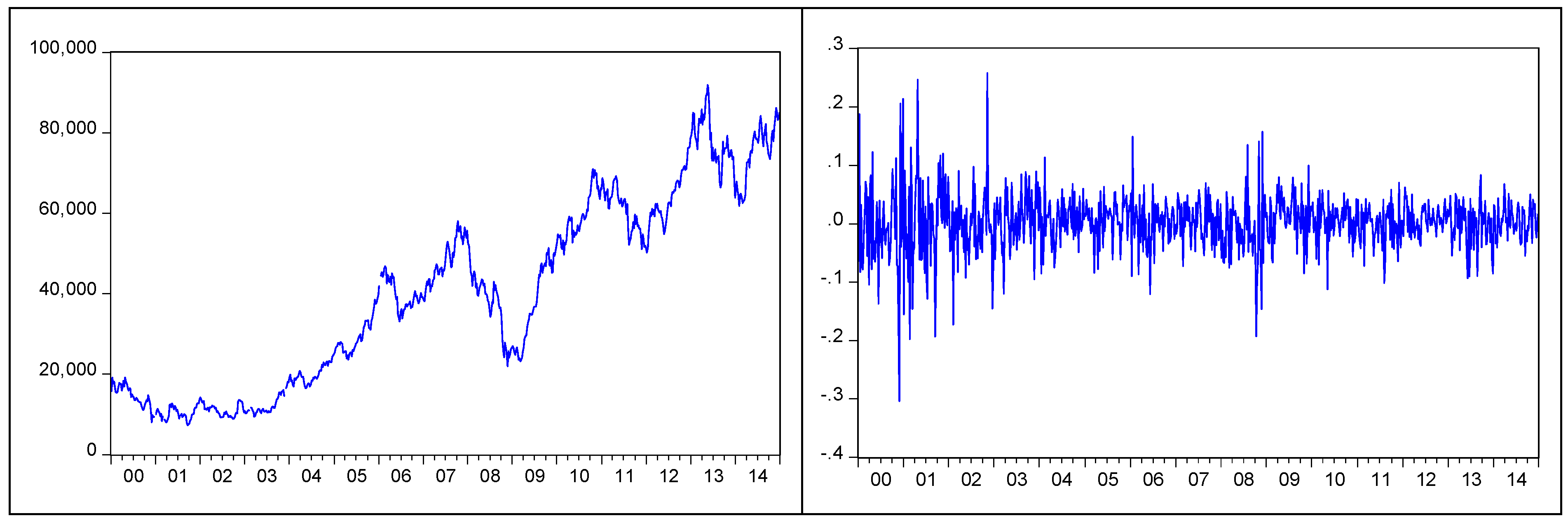
Weekly returns of 2 January 2004–26 December 2014 period of the Borsa Istanbul BIST100 index are used in the study. The data are taken weekly from the Turkish Central Bank Electronic Fund Transfer System. The return (yt) data is calculated by dividing the price index by the preceding period and taking the natural logarithm
Following Skalin and Teräsvirta (1999), returns are not seasonally adjusted. Price and return graphs of BIST 100 index for defined period is shown on Figure 1. Bai-Perron tests of L + 1 vs. L sequentially determined breaks (2003) for multiple breakpoints finds no structural breakpoints in return data series and listed in the Table 1.
Analysis of the returns of 2004–2014 with the LSTAR, ARCH, AR, and random walk, out-of-sample estimations for 12 terms (weekly) of 2015 is done with one step ahead method through each model. Methods used in obtaining optimal forecast are generally used to measure how far away the forecast is from actual return. Here, the purpose is to find the model that minimizes the difference between forecasted and actual returns. Forecast successes of the models are defined with the mean absolute error (MAE), root mean square error (RMSE), and mean absolute percentage error (MAPE) criteria. In addition, the capacity of implied directional change has also been studied, which is more important from investment point of view of all forecast models. Additionally, equal forecast accuracy is tested with the Diebold–Mariano (DM) test (Diebold and Mariano (1995)).
Before applying STAR model estimations, the order of integration of the variables has to be examined by means of the unit root test. I employ the ADF (Dickey and Fuller 1981) test for this purpose. The test maintains stochastic dynamics of the given time series and reported in the Table 2.
The paper follows STAR model estimations suggested by van Dijk (1999). Firstly, it specifies appropriate AR model with Akaike information criteria as AR(8). Then it tests STAR type nonlinearity with the LM test proposed by Luukkonen et al. (1988). Results presented in the Table 3 show that the LM test rejects the linearity in the significance degree of 1%, and the robust test rejects the linearity in the significance degree of 5%. It means that there is a STAR type nonlinear structure in the series.
In an effort to define the transition variable of the model, LM3 statistics of all candidate variables (yt−1, yt−2, ..., yt−8) are calculated and reported in the Table 4. The second lag y(t−2) is selected as a transition variable with the 0.00003669283 minimum p-value.
After selecting the transition variable, the next step is to identify the type of transition function—G(st;γ,c). In practice, the type of the function is either first degree logistic function (LSTAR), or exponential function (ESTAR). F-tests are applied to the auxiliary regression from the Taylor expansion, to identify appropriate auxiliary function. According to Teräsvirta (1994) “if p-value of the H2 hypothesis test (F2) is minimum, then ESTAR model should be selected, otherwise LSTAR model should be selected”. As shown in the Table 5, the p-value of the F version of H1 hypothesis is the minimum in the data, thus we conclude that the transition function is a logistic function—LSTAR.
Two-dimensional grid search is applied to find the starting value in the nonlinear optimization process for estimating the LSTAR model. For conducting scale-free process of γ coefficient, it was standardized through dividing by standard deviation of the series. In the estimation process of the model, statistically insignificant variables (in the 5% degree) beginning from the most insignificant ones, removed from the model, and the final nonlinear model was obtained by re-estimating the LSTAR model with the same start values. The model estimates are reported in the Table 6 below.
Nonlinear calculations with analytical gradient find γ = 60.004 and c = −0.02. As explained above, γ indicates the transition speed of regimes. Approximately, 60 is the indication of a rapid change.
Insignificance of the t-statistics of γ in the estimation results does not mean that the STAR model is invalid (van Dijk (1999, p. 31)). This univariate (logistic) transition model shows that there are two different regimes in the Borsa Istanbul in the given period. Market regimes are defined in accordance with the values of transition function. A value of 60 for the γ parameter in the logistic function shows that there is a rapid transition between the lower and upper regimes. Rapid change among regimes means that the switching from recession into expansion—i.e., recovery (or vice versa, from up to down)—is rapid.
Evaluation of estimated STAR model must be done for functionality of the model. This is tested through the diagnostics tests of STAR models proposed by Eitrheim and Teräsvirta (1996).
ARCH test results show that there is no ARCH effect in the errors in the 1% of significance degree, while there is an effect in the 5% of significance degree. Due to the extreme kurtosis and fat-tail features of the financial series, concavity and curves of the thickness do damage the reliability of the model (Çağlayan and Dayıoğlu 2009). Results of the parameter constancy test shows that the parameters in the transition functions of the defined LSTAR model are constant in accordance with the theory.
Diagnostic tests show that this model may be used in the estimation process. Additional ESTAR model was also estimated for these variables, but the insignificance of parameter coefficients and examination tests indicated that the model is not suitable.
Using the estimated LSTAR parameters, the model equation may be written as follows, where scale-free process was conducted by dividing γ by standard deviation of the transition variable
As seen in the equation, transition function of the model is in the form
Function threshold value is −0.022. Model shows that the transition variable () of BIST100 return, i.e., returns from two weeks ago determine moving between two different regimes for being higher or lower than the threshold value (−0.022).
After returns of 2004–2014 period are analyzed and modeled, with those models 12 term (3 weeks) returns of 2015 are forecasted. Estimation error of the model is calculated with mean absolute error (MAE), root mean square error (RMSE), mean absolute percentage error (MAPE) criteria. Moreover, the capacity of the implied directional change is also examined. LSTAR model forecasts estimations are listed in the Table 7.
Linear AR, ARCH(2), and random walk models’ forecasts are compared in the conclusion.
4. Conclusions
In this paper, to compare out of sample forecast power of the LSTAR, AR, ARCH, and random walk models, 12 term forecasts are made for 2015 and the MAE, RMSE, MAPE error criteria for each model, correlation coefficient between actual and estimated values are calculated, Diebold–Mariano forecast accuracy tests are applied.
As seen in the comparative values of the models described in the Table 8, the minimum value of the standard error of the model is firstly observed in the random walk, then in the LSTAR, AR, and ARCH (2) model.
While comparing models due to forecast performance, it seems that the minimum value of the mean absolute error (MAE) is at the LSTAR model. This value is lower than the random walk MAE value and ARCH(2) model MAE value. This shows that LSTAR model forecasts the market better. The minimum value in the root mean square error criteria belongs to LSTAR model. ARCH(2) model also demonstrates better performance than the random walk. Better performance in the mean absolute percentage error is observed in the LSTAR model. According to this criteria, ARCH(2) model outperformed random walk. These results show that there is a nonlinear structure in the Borsa Istanbul market in the studied period and nonlinear models outperform linear models in forecasting. This shows that the market is not weak form efficient in the studied period.
To see forecast accuracy of the LSTAR, ARCH(2), AR, and random walk models, Diebold–Mariano (DM) equal estimation accuracy test results are reported in the Table 9.
In the table we see DM test statistics is 2.072 and probability value is 0.041 in comparison of the LSTAR and ARCH (2) model, by rejecting the hypotheses of having equal forecast accuracy, it means that the forecast success of LSTAR and ARCH(2) models is different. In addition, the negative value of the test statistics means that the forecast capacity of the LSTAR model is better than the ARCH(2) model. DM test statistics is calculated as −2.973 for LSTAR and random walk models, while p-value (0.001) is less than the significance degree (0.05). LSTAR model statistically outperforms random walk, and the forecast success differs from one another. Briefly, Diebold–Mariano test shows that forecast and performance of the models are accurate at 5% significance degree.
The capacity of determining the change direction (positive of negative) of models that are more important from the investors’ point of view is also accurate. LSTAR and random walk models predict 67% of the total changes, while ARCH(2) model is successful in predicting 75% of them. LSTAR and ARCH(2) models are successful in predicting the whole (100%) of the return increase, while random walk is successful in predicting 75% of them. However, the case is a little bit different from the point of view of the losses. LSTAR model could not predict any of the losses (negative return), while ARCH(2) model was successful in predicting 25% and random walk 50% of them. Success in implied directional change shows power of signaling profit opportunities.
Correlation coefficients between actual and forecasted values are also considered. The highest correlation in actual prices is observed among the estimation of LSTAR model (0.468093). The second, third, and minimum correlation are the estimations of random walk, ARCH(2), and AR models respectively. These results show that the BIST100 index returns exhibit the nonlinear pattern and the LSTAR model of the market provides better forecasts.
The paper figures out the existence of nonlinear structure in the Borsa Istanbul index return within the studied period. The results show that the shareholders may earn excess return and identify the direction of the return change for the next week at least 66% accuracy. As a result of this, on the contrary of the linear level studies, these findings show that the Borsa Istanbul is not weak form efficient at a nonlinear level in the studied period.
The findings show the existence of nonlinear dependence in the conditional mean, as well as nonlinear structure in the conditional variance in Borsa Istanbul and this dependence may successfully be simulated with the ARCH(2) model. This is another indicator of inefficiency of weak form in Borsa Istanbul.
If the results of this paper and the findings of all other nonlinear studies are incorporated into prices, there will be a reduction in the ways to ‘beat’ the market and a significant contribution to the efficiency of Borsa Istanbul. Findings once again show the evidence of nonlinear structure at financial time series and such patterns may be modeled employing nonlinear models. Even investment companies or individual investors may apply nonlinear analysis approaches to predict emerging markets and decide on their positions.
Acknowledgments
I am grateful to Mubariz Hasanov and Alovsat Muslumov for their support and inspiration in nonlinear research, as well as to Richard Ajayi for his recommendations. Finally, the views expressed in this paper are those of the author and do not necessarily represent the views of their affiliated institutions.
Conflicts of Interest
The author declares no conflict of interest.
References
- Aliyev, Fuzuli, and Nigar Gamarli. 2018. Borsa İstanbul’da Haftaiçi Anomalisi üzerine bir İnceleme. Finans Ekonomi ve Sosyal Araştırmalar Dergisi (FESA) 3: 625–32. [Google Scholar] [CrossRef]
- Alpar, Orcan, and Özge Eren. 2016. İMKB100 Endeks Değişim Değerlerinde Lyapunov Üsteli Metoduyla Kaosun Incelenmesi. İstanbul Aydın Üniversitesi Dergisi 8: 151–74. [Google Scholar]
- Balcilar, Mehmet, Rangan Gupta, and Zahra B. Shah. 2011. An in-sample and out-of-sample Empirical Investigation of the Nonlinearity in House Prices of South Africa. Economic Modeling 28: 891–99. [Google Scholar] [CrossRef]
- Basu, Sanjoy. 1977. Investment Performance of Common Stocks in Relation to their Price-Earnings Ratios: A Test of the Efficient Market Hypothesis. The Journal of Finance 32: 663–82. [Google Scholar] [CrossRef]
- Bildirici, Melike E., Elçin Aykaç Alp, Özgür Ö. Ersin, and Ümit Bozoklu. 2010. İktisatta Kullanılan Doğrusal Olmayan Zaman Serisi Yöntemleri. Istanbul: Türkmen kitabevi. [Google Scholar]
- Busetti, Giorgio, and Matteo Manera. 2003. STAR-GARCH Models for Stock Market Interactions in the Pacific Basin Region, Japan and US. FEEM Working Paper No. 43.2003. Available online: https://ssrn.com/abstract=419081 (accessed on 15 March 2019).[Green Version]
- Busse, Jeffrey A., and T. Clifton Green. 2002. Market Efficiency in Real Time. Journal of Financial Economics 65: 415–37. [Google Scholar] [CrossRef]
- Çağlayan, Ebru, and Tuğba Dayıoğlu. 2009. Döviz Kuru Getiri Volatilitesinin Koşullu Değişen Varyans Modeleri ile Öngörüsü. Ekonometri ve İstatistik 9: 4. [Google Scholar]
- Campbell, John Y., Andrew W. Lo, and Craig MacKinlay. 1997. The Econometrics of Financial Markets. Princeton: Princeton University Press. [Google Scholar]
- Dickey, David A., and Wayne A. Fuller. 1981. Likelihood Ratio Statistics for Autoregressive Time Series with a Unit Root. Econometrica 49: 1057–72. [Google Scholar] [CrossRef]
- Diebold, Francis X., and Roberto S. Mariano. 1995. Comparing predictive accuracy. Journal of Business and Economic Statistics 13: 253–63. [Google Scholar]
- Edelen, Roger M. 1999. Investor flows and the assessed performance of open-end mutual funds. Journal of Financial Economics 5: 439–66. [Google Scholar] [CrossRef]
- Eitrheim, Øyvind, and Timo Teräsvirta. 1996. Testing the adequacy of smooth transition autoregressive models. Journal of Econometrics 74: 59–75. [Google Scholar] [CrossRef]
- Engle, Robert F. 1982. Autoregressive conditional heteroscedasticity with estimates of the variance of United Kingdom inflation. Econometrica 50: 987–1007. [Google Scholar] [CrossRef]
- Fama, Eugene. 1970. Efficient Capital Markets: A Review of Theory and Empirical Work. The Journal of Finance 25: 383–417. [Google Scholar] [CrossRef]
- Franses, Philip Hans, and Dick van Dijk. 2000. Nonlinear Time Series Models in Empirical Finance. Cambridge: Cambridge University Press. [Google Scholar]
- Gozbasi, Onur, Ilhan Kucukkaplan, and Saban Nazlioglu. 2014. Re-examining the Turkish Stock Market Efficiency: Evidence from Nonlinear Unit Root Tests. Economic Modeling 38: 381–84. [Google Scholar] [CrossRef]
- Harvey, Campbell R. 1995. Predictable risk and returns in emerging markets. Review of Financial Studies 8: 773–816. [Google Scholar] [CrossRef]
- Hasanov, Mübariz, and Tolga Omay. 2008. Nonlinearities in Emerging Stock Markets: Evidence from Europe’s Two Largest Emerging Markets. Applied Economics 40: 2645–58. [Google Scholar] [CrossRef]
- Jensen, Michael C. 1978. Some anomalous evidence regarding market efficiency. Journal of Financial Economics 6: 95–101. [Google Scholar] [CrossRef]
- Karan, Mehmet Baha, and Halit Gonenc. 2003. Do Value Stocks Earn Higher Returns than Growth Stocks in an Emerging Market? Evidence from the Istanbul Stock Exchange. Journal of International Financial Management and Accounting 14: 1–26. [Google Scholar]
- Kim, Sei-Wan, André V. Mollick, and Kiseok Nam. 2008. Common Nonlinearities in Long-horizon Stock Returns: Evidence from G-7 Stock Markets. Global Finance Journal 19: 19–31. [Google Scholar] [CrossRef]
- Koy, Ayben. 2017. Regime Dynamics of Stock Markets in the Fragile Five. Journal of Economic & Management Perspectives 11: 950–58. [Google Scholar]
- Kumar Narayan, Paresh. 2005. Are the Australian and New Zealand stock prices nonlinear with a unit root? Applied Economics 37: 2161–66. [Google Scholar] [CrossRef]
- Luukkonen, Ritva, Pentti Saikkonen, and Timo Teräsvirta. 1988. Testing linearity against smooth transition autoregressive models. Biometrika 75: 491–99. [Google Scholar] [CrossRef]
- McMillan, David G. 2005. Nonlinear dynamics in international stock market returns. Review of Financial Economics 14: 81–91. [Google Scholar] [CrossRef]
- Metghalchi, Massoud, Massomeh Hajilee, and Linda A. Hayes. 2018. Return Predictability and Efficient Market Hypothesis: Evidence from Iceland. The Journal of Alternative Investments 21: 68–78. [Google Scholar] [CrossRef]
- Rosenberg, Barr, Kenneth Reid, and Ronald Lanstein. 1985. Persuasive Evidence of Market Inefficiency. The Journal of Portfolio Management 11: 9–16. [Google Scholar] [CrossRef]
- Skalin, Joakim, and Timo Teräsvirta. 1999. Another look at Swedish business cycles, 1861–1988. Journal of Applied Econometrics 14: 359–78. [Google Scholar] [CrossRef]
- Sülkü, Seher Nur, and E. Ürkmez. 2018. Hisse Senedi Getirilerinde Doğrusal Olmayan Dinamikler: Türkiye’den Kanıtlar. Uluslararası İktisadi ve İdari İncelemeler Dergisi 18: 473–84. [Google Scholar] [CrossRef]
- Suresh, K. G., Anto Joseph, and Garima Sisodia. 2013. Efficiency of Emerging Stock Markets: Evidences from BRICS Stock Indices Data using Nonlinear Panel Unit Root Test. Journal of Economic and Financial Modeling 1: 56–61. [Google Scholar]
- Teräsvirta, Timo. 1994. Specification, estimation, and evaluation of smooth transition autoregressive models. Journal of the American Statistical Association 89: 208–18. [Google Scholar]
- van Dijk, Dick D. J. C. 1999. Smooth Transition Models: Extensions and Outlier Robust Inference. Tinbergen Institute Research Series No. 200; Rotterdam: Erasmus University Rotterdam. [Google Scholar]
| 1 | Statistically insignificant variables are removed. |
Figure 1.
BIST100 index price (left) and return (right) series graph.


Table 1.
Multiple breakpoint tests.
| Bai-Perron tests of L + 1 vs. L sequentially determined breaks | |||
| Sequential F-statistic determined breaks: | 0 | ||
| Scaled | Critical | ||
| Break Test | F-statistic | F-statistic | Value |
| 0 vs. 1 | 2.935485 | 2.935485 | 8.58 |
Table 2.
Unit root test results.
| Null Hypothesis: RTRN has a unit root | ||
| t-Statistic | Prob. | |
| Augmented Dickey–Fuller test statistic | −19.82786 | 0.0000 |
Table 3.
Luukkonen et al. STAR type nonlinearity test results.
| F-Stat | p-Value | χ2-Stat | p-Value | |
|---|---|---|---|---|
| LM test | 3.6247 | 0.0012149 | 20.921 | 0.0015951 |
| Robustness test | 2.3781 | 0.0186173 | 15.036 | 0.0184397 |
Table 4.
p-values of LM3 test statistics of the candidate transition variables.
| Lag | y(t−1) | y(t−2) | y(t−3) | y(t−4) |
| p-value | 0.00010439 | 0.0000036692 | 0.0016405 | 0.0038045 |
| Lag | y(t−5) | y(t−6) | y(t−7) | y(t−8) |
| p-value | 0.098301 | 0.058143 | 0.0024708 | 0.28923 |
Table 5.
Transition function identification test results.
| Test | Test Statistics (F) | p-Value | df |
|---|---|---|---|
| LM.H1 | 3.620 | 0.0004045 | 8 |
| LM.H2 | 3.607 | 0.0004294 | 8 |
| LM.H3 | 1.523 | 0.1462000 | 8 |
Table 6.
Estimated LSTAR models and statistics1.
Table 6.
Estimated LSTAR models and statistics1.
| Parameter | Coef. | Std. Error | t-Stat. | Prob. (p) |
|---|---|---|---|---|
| Gamma | 60.004 | 134.679 | 0.446 | 0.655 |
| Threshold | −0.022 | 0.001 | −16.532 | 0.001 |
| Linear Part | ||||
| Constant | 0.009 | 0.006 | 1.517 | 0.029 |
| AR(4) | −0.191 | 0.094 | −2.027 | 0.042 |
| AR(7) | −0.249 | 0.084 | −2.936 | 0.003 |
| AR(8) | 0.168 | 0.102 | 1.647 | 0.048 |
| Nonlinear Part | ||||
| AR(1) | 0.437 | 0.091 | 4.794 | 0.001 |
| AR(7) | 0.174 | 0.098 | 1.776 | 0.045 |
Table 7.
LSTAR model out-of-sample forecasts.
| Date | LSTAR Model Estimations | Actual Values |
|---|---|---|
| 02.01.2015 | 0.001667 | 0.001292 |
| 09.01.2015 | 0.015832 | 0.024908 |
| 16.01.2015 | 0.002133 | 0.007809 |
| 23.01.2015 | 0.014733 | 0.023102 |
| 30.01.2015 | 0.016794 | 0.002778 |
| 06.02.2015 | 0.00122 | −0.03732 |
| 13.02.2015 | 0.002241 | −0.02543 |
| 20.02.2015 | 0.012025 | 0.011279 |
| 27.02.2015 | 0.009967 | 0.004584 |
| 06.03.2015 | 0.001158 | −0.04368 |
| 13.03.2015 | 0.014974 | −0.04874 |
| 20.03.2015 | 0.013324 | 0.027095 |
| MAE | 0.019348 | |
| RMSE | 0.027267 | |
| MAPE | 1.082635 | |
| D (n = 12) | 66.67% | |
| 100% | ||
| 0% | ||
| Correlation | 0.468093 | |
Table 8.
Comparative statistics of estimation models.
| LSTAR | ARCH(2) | AR | Random | |
|---|---|---|---|---|
| Standard error | 0.030842 | 0.032263 | 0.031976 | 0.001383 |
| MAE | 0.019348 | 0.021613 | 0.020948 | 0.027887 |
| RMSE | 0.027267 | 0.027568 | 0.027373 | 0.034015 |
| MAPE | 1.082635 | 1.319568 | 1.090293 | 3.959061 |
| D (n = 12) | 66.67% | 75% | 66.67% | 66.67% |
| 100% | 100% | 87.5% | 75% | |
| 0% | 25% | 25% | 50% | |
| Correlation coefficient | 0.468093 | 0.079124 | −0.00621 | 0.170788 |
Table 9.
Diebold–Mariano test results.
| LSTAR | ARCH(2) | Random Walk | AR | |
|---|---|---|---|---|
| LSTAR | − | −2.072 (0.041) | −2.973 (0.001) | −2.258 (0.035) |
| ARCH(2) | − | − | −1.992 (0.043) | −2.617 (0.002) |
| Random Walk | − | − | − | 1.9115 (0.047) |
| AR | − | − | − | − |
© 2019 by the author. Licensee MDPI, Basel, Switzerland. This article is an open access article distributed under the terms and conditions of the Creative Commons Attribution (CC BY) license (http://creativecommons.org/licenses/by/4.0/).
Share and Cite
MDPI and ACS Style
Aliyev, F. Testing Market Efficiency with Nonlinear Methods: Evidence from Borsa Istanbul. Int. J. Financial Stud. 2019, 7, 27. https://doi.org/10.3390/ijfs7020027
AMA Style
Aliyev F. Testing Market Efficiency with Nonlinear Methods: Evidence from Borsa Istanbul. International Journal of Financial Studies. 2019; 7(2):27. https://doi.org/10.3390/ijfs7020027
Chicago/Turabian StyleAliyev, Fuzuli. 2019. "Testing Market Efficiency with Nonlinear Methods: Evidence from Borsa Istanbul" International Journal of Financial Studies 7, no. 2: 27. https://doi.org/10.3390/ijfs7020027
Note that from the first issue of 2016, this journal uses article numbers instead of page numbers. See further details here.