
A Data Cube Metamodel for Geographic Analysis Involving Heterogeneous Dimensions


1
SPHERES, Geomatics Unit, University of Liege, 4000 Liège, Belgium
2
SPHERES, SEGEFA, University of Liege, 4000 Liège, Belgium
*
Author to whom correspondence should be addressed.
ISPRS Int. J. Geo-Inf. 2021, 10(2), 87; https://doi.org/10.3390/ijgi10020087
Submission received: 1 December 2020
/
Revised: 21 January 2021
/
Accepted: 17 February 2021
/
Published: 19 February 2021
(This article belongs to the Special Issue GIS Software and Engineering for Big Data)
Abstract
:Due to their multiple sources and structures, big spatial data require adapted tools to be efficiently collected, summarized and analyzed. For this purpose, data are archived in data warehouses and explored by spatial online analytical processing (SOLAP) through dynamic maps, charts and tables. Data are thus converted in data cubes characterized by a multidimensional structure on which exploration is based. However, multiple sources often lead to several data cubes defined by heterogeneous dimensions. In particular, dimensions definition can change depending on analyzed scale, territory and time. In order to consider these three issues specific to geographic analysis, this research proposes an original data cube metamodel defined in unified modeling language (UML). Based on concepts like common dimension levels and metadimensions, the metamodel can instantiate constellations of heterogeneous data cubes allowing SOLAP to perform multiscale, multi-territory and time analysis. Afterwards, the metamodel is implemented in a relational data warehouse and validated by an operational tool designed for a social economy case study. This tool, called “Racines”, gathers and compares multidimensional data about social economy business in Belgium and France through interactive cross-border maps, charts and reports. Thanks to the metamodel, users remain independent from IT specialists regarding data exploration and integration.
1. Introduction
Big data has become a very active research field considering the fast increasing of data sources diversity: sensors, smartphones, crowdsourcing, social networks, open databases, etc. These numerous and large datasets are thus characterized by heterogenous semantics, structures and formats leading to time-consuming processes for management and analysis purposes. Management and analysis also have to deal with multidimensional aspects of information characterized by space, time and any other analysis axis proper to specific domains like category of a product, size of a company, age of a population, etc.
On the one hand, heterogeneous data structures have led to a large panel of technologies for their management: relational databases, document stores, graphs, data cubes, data lakes, etc. On the other hand, powerful tools allow the gathering and the analysis of data in order to create valuable information. Big data analysis can be performed by machines in promising fields like artificial intelligence, machine learning, deep learning, etc. However, big data analysis by humans is still an important issue. Unlike machines, humans need summarized representations of data to take relevant decisions. This aspect on which this research is based is called business intelligence (BI). It requires “Extract, Transform, Load” (ETL) tools to transform data structures, data warehouses to archive them in a common multidimensional structure and online analytical processing (OLAP) to explore them through interactive tables, charts or maps.
Among big data, around 80% have a spatial component [1]. This opens the door to geographic analysis and its specific issues related to heterogeneous data. We identify three of them. First, a central principle of geography is multiscale analysis. Indeed, a spatial phenomenon must be analyzed at different scales for its global understanding (e.g., street, district, city, region, country). However, available data can be more or less detailed depending on their aggregation level. For example, French economics data showing number of workers per company size are available at department scale but not at commune scale due to statistical confidentiality. Secondly, territories comparison can be biased by data definitions differing in these territories. For example, categorization of companies regarding their activity area are different in France and Belgium. Eventually, geography also includes temporal analysis which is subject to changes in data dimensions. For example, the number of Belgian communes decreased from 589 to 581 due to administrative fusions in 2019.
Geographic analysis is very interdisciplinary because it can be performed in numerous fields involving spatial data: marketing, criminology, archeology, ecology, oceanography, urban planning, etc. All these fields have their own experts who might need to analyze and explore big geospatial data. However, exploration tools require adapted skills in data modelling and programming to process data. Due to previously mentioned issues related to geographic analysis, expert users of a specific field might stay dependent on IT specialists to durably use exploration tools like OLAP.
The objective of this research is the development of a BI infrastructure for the geographic analysis of multidimensional and heterogeneous data. It is intended for social economy specialists who want to stay independent of IT specialists regarding data integration, exploration and analysis. Therefore, the design must be based on a data metamodel considering the three issues of geographic analysis previously mentioned: multiscale analysis, multi-territory analysis and time analysis.
The paper is structured as follows. In Section 2, we review literature related to economic geography analysis, BI and OLAP. Section 3 reviews literature related to OLAP metamodels and the three specific issues of geographic analysis: multiscale analysis, multi-territory analysis and time analysis. In Section 4, we briefly present our social economy case study and we formulate our research hypothesis. In Section 5, we present our original metamodel followed by its relational implementation in Section 6. In Section 7, the metamodel is validated by the BI web platform dedicated to the integration and the geographic analysis of multidimensional data about social economy companies and workers. Eventually, we conclude this paper in Section 8.
2. Background
This section is devoted to a review of the literature relevant to our research objective. It starts with main concepts of economic geography analysis since our tool is designed for this purpose (Section 2.1). Section 2.2, Section 2.3, Section 2.4 and Section 2.5 are devoted to OLAP regarding BI infrastructures, Spatial OLAP (SOLAP), OLAP implementation and OLAP modeling.
2.1. Economic Geography Analysis
Economic geography has long been committed to defining and studying the concepts of learning, innovation and economic governance in relation with territories and geographic space. This approach would not have been possible without geographic information systems (GIS) and their ability to integrate various spatial datasets based on spatial coordinates.
A fundamental debate in economic geography is whether places are more relevant to the competitiveness of firms, or whether networks are more important [2]. The concept of “space of places” expresses the idea that the location matters for learning and innovation, while networks are important vehicles of knowledge transfer and dissemination [3]. However, this debate has not been a real issue in the literature about innovation clusters until quite recently. The networks are associated with inter-firm settings in which knowledge creation, dissemination and innovation take place [4]. These ideas resonate with multiple fields of research in economic geography by focusing on economic action in a relational and dynamic way. This includes geography of practice [5], evolutionary economic geography [6] and relational economic geography [7]. The tool developed in this research responds to the needs of a project (VISES or “Valorisation de l’Impact Social de l’Entrepreneuriat Social”, see Section 4.1) following a similar methodology. Different datasets about social economy companies are gathered to study their contribution to territorial dynamics.
2.2. Business Intelligence and Online Analytical Processing (OLAP)
Business intelligence (BI) refers to a collection of tools for the exploration and analysis of large datasets [8]. As shown in Figure 1, a typical BI infrastructure includes heterogeneous data sources which are connected to a data warehouse through ETL systems [9]. ETL allows the automatization of data transformations to a multidimensional structure which is the common paradigm used for data exploration and analysis. Indeed, big data are characterized by important volume, variety and complexity requiring adapted tools for their collect and storage [10].
A data warehouse (DW) archives multidimensional data by following an OLAP approach [11,12]. Contrary to online transactional processing (OLTP), OLAP involves complex but fast aggregations processes in order to summarize data in tables or charts. This aspect can possibly be handled by storing different versions of a same dataset at different aggregation levels of a dimension hierarchy (e.g., data per year, data per month, data per week, etc.). This redundancy does not affect the consistency of the system since OLAP only archives data in time and never requires updates. Indeed, only new data can be inserted in a DW and archived data are not supposed to evolve.
DW exploration and analysis is performed by OLAP tools. These interpret the multidimensional structure of data in order to effectively represent them in user-friendly interfaces. Data are thus modeled as data cubes (or data marts) characterized by dimension axis (e.g., time, location, type of product, etc.) indexing variables (or measures) which can be represented in dynamic tables or charts. For example, a measure can be a number of sales, a number of people or a molecule concentration depending on time, location and various typologies. An OLAP dynamic interface allows end-users to freely navigate in data cubes by performing operations like:
- respectively allocating dimensions to the rows and columns of a pivot table [13];
- allocating a measure to the cells of a pivot table;
- roll up/drill down in a dimension hierarchy (e.g., switching between levels “year” and “month” of a time dimension) and consequently aggregate measures;
- slice a dimension (e.g., only consider measures attached to month “November 2020” of time dimension).
In addition to free exploration, OLAP systems can also supply reporting tools. These are static outputs like pdf (“portable document format”) files or web dashboards showing specific precomputed data representations. For example, a report can include a chart representing sales by weeks and product type which is automatically updated every week (when new data are archived in the DW). The analytical potential is less powerful than in OLAP free exploration but it directly shows the important trends of data without requiring any action from the end-user. Indeed, data free exploration can sometimes be confusing for uninformed users, especially when data dimensions are numerous [14].
2.3. Spatial Online Analytical Processing (SOLAP)
Spatial OLAP (SOLAP) introduces spatialization of OLAP concepts for geographic analysis purpose [15]. Therefore, a spatial data cube can include spatial dimensions whose elements (members) are characterized by a spatial definition like coordinates of vector entities [16]. For example, a spatial dimension can include administrative entities like countries associated to georeferenced polygons. Spatial dimensions allow representations of data in interactive maps as well as SOLAP operations like spatial drill down in a spatial dimension hierarchy (an example is given in Section 5.1, Figure 8). Multiscale analysis and territories comparisons can thus be efficiently managed by SOLAP for homogeneous data. Moreover, SOLAP can benefit from both multidimensional analysis, provided by OLAP, and spatial analysis, provided by GIS. This leads to original SOLAP operations like OLAP-buffer or OLAP-overlay detailed in [17,18]. This research also proposes the term “geographic dimension” instead of “spatial dimension” since these dimension members include both a semantic definition (e.g., Belgium country) and a spatial definition (e.g., a polygon representing the Belgian border). The remainder of this paper follows this proposition.
SOLAP can be useful in various domains like pollutant analysis [17], crime analysis [19], risk analysis [20], mobility [21], forestry [22], healthcare [23], epidemiology [24], etc. Nevertheless, some domains can require adapted SOLAP models in order to fit to the needs of the application. For example, the usual association of vector finite entities to geographic dimensions is not adapted to domains requiring a continuous vision of space (field) [25]. For this purpose, an alternative definition of spatial dimensions is proposed in [19]: geographic dimensions remain classical SOLAP dimensions attached to spatial features while spatial dimensions are X and Y axis of a coordinate reference system. This model can be implemented using raster data in order to manage continuous fields in a SOLAP.
2.4. OLAP Implementation
OLAP data cubes can be implemented following different strategies. The most popular ones are multidimensional OLAP (MOLAP) and relational OLAP (ROLAP) [26].
On the one hand, MOLAP appears to be the most obvious strategy since it stores and manages data cubes as multidimensional arrays. MOLAP operations are thus relatively easy since their implementation is very close to their conceptual definition. Nevertheless, MOLAP efficiency depends on data cubes density. Indeed, when they are characterized by numerous and detailed dimensions, MOLAP data cubes are likely to store a large amount of useless null values (low density issue). Indeed, some data cubes’ cells, i.e., dimension intersections or facts, do not exist in data. In GIS domain, this problem is quite similar to raster data including numerous “no data” values [19].
On the other hand, ROLAP uses relational data warehouses to store data cubes [11]. Data cube cells are rows of a fact table which do not require storage for null values. Thus, ROLAP efficiently manages data cubes involving numerous and detailed dimensions but they require complex SQL (structured query language) queries for multidimensional representation in OLAP interfaces. This aspect can be managed by a dedicated OLAP tools like Mondrian [27] or PowerBI [28] which allow querying relational data warehouses through MDX (MultiDimensional eXpression) language.
2.5. OLAP Modeling
Due to multiple implementation strategies, it is important to describe (S)OLAP modeling at a conceptual level. According to this principle, the well-known star schema [11] describes a multidimensional dataset using OLAP concepts like dimension, fact, measure, etc. Moreover, multiple datasets can be described by a constellation schema [22] which is basically a set of star schemas sharing common elements like measures or dimensions. It allows comparisons between heterogeneous data cubes through drill across operations [34].
Numerous SOLAP studies use a graphic notation to represent star schema models. Some use a dedicated multidimensional formalism [21,35]. Others use standard unified modeling language (UML) class diagram to describe star schemas (or a very close formalism) [12,22,36]. Amongst these, some propose UML extensions (UML profiles) to be able to describe specificities required by OLAP [37,38]. Others describe a generic star schema using a UML data cube metamodel [39,40,41]. In data cube metamodels, OLAP concepts such as dimensions, dimension levels, hierarchies or measures are modeled through metaclasses as shown in Figure 2 example. These metaclasses allow the automatic instantiation of star schemas based on parameters defined by users. Instantiated star schemas can possibly be connected by common dimensions and/or measures in order to model complex constellations of heterogeneous data cubes. Thanks to metamodel parameters stored in the DW, constellations structures can be interpreted by a dedicated (S)OLAP tool for exploration and comparison purposes.
3. Related Work
The three identified issues of geographic analysis involving heterogeneous dimensions, i.e., time analysis (1), multi-territory analysis (2) and multiscale analysis (3), can be reformulated by the management of data cubes related to heterogeneous dimensions which are likely to change in time, geographic space and geographic scale. The authors of [42] point out that issues 1 (“Handling change and time”) and 3 (“Handling different levels of granularity”) are rarely present in existing OLAP models (issue 2 is not identified by authors). Regarding concepts previously described, Section 3.1 reviews OLAP literature related to these three issues. Since this paper proposes a solution based on a data cube metamodel, Section 3.2 focuses on this specific aspect. Eventually, Section 3.3 gives a brief synthesis of these literature reviews in order to define our contribution to SOLAP domain.
3.1. OLAP Constellations and Heterogeneous Dimensions
The integration of evolving dimensions (i.e., dimensions changing in time) in data warehouses has been an important research topic for the past 20 years, leading to the concept of temporal data warehouses (TDW) [43]. The main idea of TDW is the storage a valid time attribute (time point, time interval or temporal element) related to any element of an instantiated multidimensional model (i.e., member, fact, etc.) or metamodel (i.e., level, hierarchy, dimension, data cube, etc.). Therefore, SDT support evolving instances as well as schemas and OLAP can return consistent results based on multiple periods and versions of dimensions [44]. However, since queries are based on a temporal topology, these solutions are not adapted to dimensional changes depending on other dimensions than time (space or other thematic dimensions).
In [22], an alternative solution is proposed to integrate evolving dimensions in a DW: a constellation schema where each data cube, related to a time member, is associated to “generic dimensions” (i.e., shared by other data cubes) and “specific dimensions” (i.e., specific to the involved data cube and thus depending on time). In addition to evolving dimensions (time analysis issue), we believe that a constellation could also consider dimensional changes depending on geographic space (multi-territory analysis issue). Indeed, the dependency of data cubes on dimension members referring to time could actually be transposed to any other dimension members, including geographic ones. Compared to a single star schema, evolving dimensions in constellations offer low data cube densities which are easily handled by both MOLAP and ROLAP systems according to [22]. Nevertheless, this solution requires an effective management of constellation navigation in order to select the right data cube(s) answering to a user query. Unfortunately, this aspect is not covered by [22] but could possibly be handled by an adapted metamodel.
In [45], a graphical formalism is proposed to support the conceptual modeling of a DW. Multidimensional structures are modeled as quasi-tree graphs called “fact schemes” which can be overlapped to support drill-across queries. The authors discuss the possibility to include time as a dimension of their model to handle evolving schemas. Again, this idea could be extended to space regarding dimension definitions depending on territories.
In [46], a user-oriented algebra is proposed to define OLAP operations based on a multidimensional constellation. However, most of described operations are limited to navigation inside a single data cube (roll up, drill down, rotate, etc.). The only exploitation of constellation lies in selections of a specific data cubes (“DISPLAY”) and typical drill-across operations (“FROTATE”) to compare facts sharing dimensions. Navigation in constellation through operations on heterogeneous dimensions (e.g., time-varying dimension) is not considered.
In addition to shared dimensions, some interesting studies demonstrate that constellations can be characterized by more flexible inter-stellar relationships. In [47,48], drill across operations use semantical similarities between different dimensions (dimension–dimension), different facts (fact–fact) or dimensions and facts (dimension–fact). These relationships are grouped in three categories: generalization, association and derivation. Following this approach, we believe that fact–fact relationships could also be categorized as aggregations defined by a dimension hierarchy. We propose to model this as constellations where data cubes share dimension levels (instead of traditional shared dimensions). Consequently, constellations could be navigated through inter-stellar spatial roll up and spatial drill down operations when shared levels are geographic (multiscale analysis issue).
3.2. Data Cube Metamodels
Basically, OLAP metamodels store metadata related to data warehouses for interoperability purposes. According to this principle, the Object Management Group (OMG) proposes a standard called Common Warehouse Metamodel (CWM) [49]. CWM aims at integrating data warehousing and BI tools based on shared metadata. It uses XMI (XML Metadata Interchange) for metadata exchange and UML to represent various metamodels including OLAP. The OLAP metamodel proposed by CWM (Figure 3) defines multidimensional concepts (data cube, dimension, hierarchy, level, etc.) as classes connected by associations. Therefore, it could be used to help data cube integration as well as navigation in a constellation. Unfortunately, it is not compatible with our multiscale analysis issue. Indeed, the metamodel considers data cubes sharing common dimensions while dimensionality of data can also depend on specific hierarchy levels of dimensions (multiscale analysis issue). In other words, navigating in a CWM constellation through roll up and drill down is not allowed since levels are exclusive properties of dimensions [50].
Other UML metamodels are proposed in OLAP literature for various purposes. In [41], data quality of spatial DW is controlled by using integrity constraints. In [44], the COMET metamodel keeps track of modifications on multidimensional elements in a TDW. Other studies propose metamodels to help developers for data cubes design [51] or to include OLAP in more general big data architectures [40]. Eventually, more recent studies use metamodels for the automatic implementation of data cubes based on conceptual models [52] (model-driven architecture) and for the automatic instantiation of data cubes based on external data sources [39]. Like CWM, most of these UML metamodels allow data cubes to share dimensions but do not consider constellation navigation in greater depth.
3.3. Synthesis
This literature review shows that time-variation of OLAP dimensions has been well covered during the past 20 years. However, variations of dimensions depending on space and geographic scale are much less studied but could possibly be handled by an adapted constellation. On the other hand, numerous works exploit UML metamodels for OLAP but, to the best of our knowledge, none of them deeply focus on their ability to lead navigation in a data cube constellation, especially considering all these three aspects of geographic analysis involving heterogeneous dimensions: multi-territory analysis, multiscale analysis and time analysis. This constitutes the main contribution of this paper to the SOLAP field.
4. Social Economy Case Study and Research Hypothesis
4.1. Social Economy Case Study
This research is part of a larger project called VISES. In a transnational approach including French region Haut-de-France as well as Belgian regions Wallonia and Flanders, it aims at “highlighting how social economy companies contribute to the dynamic of the territories and to the well-being of their inhabitants” [53]. The methodology includes the design, testing and dissemination of an appropriate system for social entrepreneurship to improve social impact. The VISES project involves various actors including social economy networks, social finance institutions and academic researchers.
The project includes the development of a web platform, called “Racines”, allowing any visitor to use SOLAP to explore social economy data. As shown in Figure 4, explorable data are imported by administrators during all the lifetime of the platform. These administrators are French [54] and Belgian [55] social economy specialists who want to remain independent of IT specialists after production. Let’s note that “Racines” also allows data sharing by companies but this aspect will not be discussed in this paper.
Social economy datasets can be related to companies or workstations. Measures about companies are number of companies, number of workstations, number of full-time equivalents and total payroll. These can depend on the following dimensions:
- company size (e.g., less than 5 workers, from 5 to 10 workers),
- activity area (e.g., agriculture, human health),
- social economy family (e.g., association, cooperative, foundation, mutual society),
- time (year),
- administrative entity (e.g., Liège province, Paris department).
In datasets about workstations, measure “number of workstations” can also depend on these additional dimensions:
- sex,
- age,
- socio-professional category (e.g., employee, worker).
In addition to multidimensional aspect of social economy data, the “Racines” SOLAP tool must face the three following issues related to data heterogeneity.
The first issue is multi-territories analysis. Indeed, a user should be able to explore maps showing both administrative entities of Belgium and France at different scale levels: level 1 includes Belgian communes and French EPCI (“Établissement public de coopération intercommunale”), level 2 includes Belgian provinces and French departments, level 3 includes Belgian regions and France regions (these levels of comparison were defined by social economy specialists based on the average size and population of the administrative entities.). However, these data are collected at a national level and consequently have different semantics. Indeed, dimension “activity area” is not the same in France than in Belgium. For example, at level 1 (EPCI and communes), Belgian data have 20 categories while French data have only 8. Moreover, these categories are defined by different vocabularies. This underscores the importance of entrusting data integration to specialists capable of establishing the right relationships between these different classifications.
The second issue is multiscale analysis which also involves semantical changes in data. Indeed, due to statistical confidentiality, French data are not available with the same level of details at each scale level. For example, the dimension “company size” is present at region and department levels but not at EPCI level. It is to be noted that both data integration and data exploration are affected by this unavailability.
The third issue is time analysis. All dimensions are likely to change in time, especially administrative entities. For example, the number of Belgian communes decreased from 589 to 581 due to administrative fusions in 2019. Other fusions are possibly planned for 2024. Another example is the evolution of dimension “activity area”, involving new categories, removed categories or semantic redefinitions of former categories in both countries. Our metamodel must, therefore, consider past changes as well as future changes in data dimensionality.
4.2. Research Hypothesis
Let’s remember the main objective of our research: the development of a user-friendly tool for the exploration and analysis of big geospatial data. In order to meet the needs of our social economy case study, the developed tool must take these aspects into account:
- Multidimensional analysis of heterogeneous data.
- Geographic analysis involving multiscale analysis, multi-territories analysis and time analysis which are likely to change other dimensions definitions (due to heterogeneous data semantics).
- Independence of end-users from IT specialists regarding data exploration and integration.
Considering previously reviewed literature, our research hypothesis is to develop a UML SOLAP metamodel able to generate interconnected star schemas (constellation) in order to navigate between heterogeneous spatial data cubes sharing common dimension levels. The metamodel should be able to find the appropriate data cubes answering to spatial drill down or roll up for multiscale analysis and drill across for time and multi-territory analysis. Afterwards, this metamodel will be implemented within a BI infrastructure including a relational data warehouse (ROLAP), a data integration module, an exploration module (SOLAP) and a reporting module.
5. Metamodel
This section is devoted to the original metamodel translated from our research hypothesis, i.e., a metamodel for the management of heterogeneous data cubes in constellations characterized by shared dimension levels. Based on SOLAP concepts presented in Section 5.1, the data cube metamodel is formalized by UML language in Section 5.2. In order to consider the issue related to multiscale analysis, an association of data cubes to dimension levels is used. Examples of data cubes instantiated by the metamodel, following two different implementation strategies, are given in Section 5.3. Eventually, Section 5.4 describes an original concept of “metadimension” considering issues related to multi-territories analysis and time analysis.
5.1. SOLAP Concepts
A data cube is characterized by a multidimensional structure which can be defined by a star schema [11]. An example is given in Figure 5. This conceptual model shows every dimension (red branches of the star) of an economic data set about companies. Each dimension is characterized by a set of members hierarchized by ordered levels (symbolized in green). For example, the dimension “Activity area” includes three levels: “All”, “Typology A” and “Typology B”. “Typology B” is the most detailed level (or simply called “detailed level”) which could include the following members: “primary education”, “secondary education”, “High education”, etc. “Typology A” is a less detailed level which could include “Education” among others. In this hierarchy, members of level “Typology B” can be children of level “Typology A” (“primary education, “secondary education”, “high education” all belong to “education”). Finally, level “all” includes only one member which is the parent of every “Typology A” members. Thanks to dimension hierarchies, OLAP drill down and roll up operations can be performed to change data granularity. Note that only simple hierarchies are considered in Figure 5 example. More complex hierarchies, like multiple hierarchies or parallel hierarchies, can be described through other formalisms [35].
Figure 5 also represents a geographic dimension (symbolized in italic), “Administrative entities”, which is characterized by geographic members. A geographic member has a semantic definition (e.g., “Liège province” name) and a spatial definition (e.g., geometry of “Liège province” [16]). Unlike other dimensions, geographic dimensions can be represented on a map (e.g., representation of level “provinces” as 2D polygons). Other dimensions can be represented in tables or charts as well as geographic dimensions thanks to their semantic definition. When OLAP is characterized by geographic dimensions, it becomes SOLAP [17]. It should be noted that time dimensions can also have a specific management regarding time cycles like hours, weeks, seasons, etc. [56].
In the center of the star schema, measures are represented in blue (e.g., “Number of companies”, “number of workers”, etc.). They are aggregated data depending on dimension members they are attached to. In our example, measures attached to a parent dimension member are the sum aggregation of its child members. For this reason, the time dimension is the only one characterized by one single level (“year”) since adding annual number of companies in “all” level does not make any sense.
Finally, the star schema represents facts which are the analyzable elements shown in the different SOLAP interfaces (tables, charts, maps). A fact is composed of one member per dimension of the star schema and a measure value can be associated to every fact. For example, a fact can be the number of companies (measure) in Liège commune (dimension “Administrative entity”) with less than 5 workers (dimension “company size”), in construction sector (dimension “activity area”), in 2019 (dimension “time”), all families included (dimension “Social economy family”). Note that a fact involving a geographic dimension is considered as geographic fact since it can be represented on a map.
A star schema instance is a data cube (or “data hypercube”). Figure 6 shows the representation of a data cube instantiated from Figure 5 star schema. Since it is not possible to graphically represent a hypercube of five dimensions, only three dimensions are considered. Nevertheless, an n dimensions data cube can efficiently be managed in a data warehouse.
A data cube is the set of every possible fact by considering one level per dimension of the star schema. In other words, a data cube of n dimensions is the cartesian product of n sets of members called “dimension levels”. Each cell of the data cube is a fact indexed by coordinate dimensions and coordinates dimensions are actually identifiers of dimension members.
All the instances of a star schema constitute a lattice of cuboids which is the set of every possible data cube based on a single star schema [18,57]. In other words, there is one cuboid for each possible combination of dimension level by considering one level per dimension (cartesian products of dimension levels). The most detailed cuboid, called basic cuboid, is defined by each most detailed level of dimension (detailed facts). In our example, the basic cuboid is defined by “commune”, “year”, “typology B”, “company size” and “family”. All other cuboids measures are aggregations of the basic cuboid. OLAP drill down and roll up operations can then be performed by navigating in the cuboid lattice. Figure 7 shows a lattice of cuboids based on these two theoretical dimensions: {A, B, all} and {1, 2, all}. Common SOLAP operations like drill down and roll up are illustrated by concrete Belgian examples in the following paragraphs
Figure 8 shows drill down and roll up on “administrative entity” dimension. As a geographic dimension, its spatial definition (geometry polygons) is represented on a map interface. “number of companies” measures associated to geographic facts are represented by a color variation of polygon geometries (level members). The drill down is performed on level “region” and more particularly on member “Vlaams Gewest”. The result is the set of geographic facts associated to members of inferior level “province” which belong to the drilled member “Vlaams Gewest”. Roll up is simply the reverse operation. In SOLAP literature, drill down and roll up applied to a geographic dimension are respectively called spatial drill down and spatial roll up. Thanks to their ability to quickly switch from a global scale to a more local scale (and vice versa), these operations are very efficient for the spatial exploration of geographic big data. In addition to map interface, spatial drill down can be performed on other interfaces (charts or tables) representing geographic dimensions and/or other non-geographic dimensions. Indeed, this ability to switch from an interface to another is a valuable advantage of SOLAP in big data exploration
It should be noted that for relevant comparisons of spatially discrete entities, measures should be independent of the surface they are attached to. They thus should be transformed to densities like companies per surface unit or companies per population unit. This aspect can be handled by “derived measure” concept explained in Section 5.2.
Finally, Figure 9 shows a slice operation in both maps (Figure 9a) and charts (Figure 9b) interfaces. On the one hand, maps show geographic level “province” resulting from drill down operation showed in Figure 8. On the other hand, charts show dimension level “company size” in rows and geographic level “region” in colors (actually, only one region is represented in blue in this example). Represented measures are still “number of companies”. Slice operations isolate subsets of data cubes based on a specific member of one or many dimensions. According to this principle, charts of Figure 9b are initially sliced by “Vlaanderen” (i.e., member of geographic level “region” represented in blue). However, the illustrated slice of the figure is the one applied on dimension “family” (i.e., social economy family) for both interfaces. Therefore, in figure’s top, represented facts are associated to all families (i.e., level “all” of dimension “family”). In figure’s bottom, a slice on member “mutual societies” of dimension “family” consequently changes represented facts definition. Slices on different dimensions can thus be combined together since the second chart interface is both sliced by “mutual societies” and “Vlaanderen” members. Slice can be performed on represented dimensions (e.g., geographic dimension in charts) or non-represented dimensions (e.g., dimension “family” in both charts and maps). Regarding non-sliced dimensions, a represented level of dimension shows all members belonging to this level (e.g., activity area in charts), while a non-represented dimension is aggregated at its “all” level (e.g., activity area in map). Consequently, a non-represented time dimension should always be sliced since it does not include any “all” level according to Figure 5 schema. Therefore, in Figure 9 the example is also sliced by the year 2015.
5.2. Data Cube Metamodel
This section is devoted to the original metamodel of this research. It is formalized as a UML class diagram in Figure 10. Based on the data cubes concepts defined in previous section, this metamodel is able to automatically generate and manage data cube instances in a constellation. In order to manage heterogeneous dimensions in multiscale analysis, multi-territories analysis and time analysis, two original approaches are proposed in the metamodel.
- In most of UML metamodels proposed in literature, data cubes are associated to dimensions. Our metamodel follows a different approach: data cubes are directly associated to dimension levels. This allows navigation between different data cubes through roll up and drill down operations. Indeed, multiscale analysis must consider changes in non-geographic dimensions depending on geographic dimension levels.
- Unlike multiscale analysis involving changes depending on dimension level, our two other objectives, i.e., multi-territories and time analysis, must consider changes depending on dimension members, i.e., time members for time analysis and geographic members for multi-territories analysis. This aspect is managed through a metadimension concept explained in Section 5.4.
Although it was developed for a specific application, i.e., exploration and reporting of social economy data, this metamodel can be used for SOLAP in other fields involving spatially discrete data. Moreover, this conceptual metamodel is not dependent on any database management system (DBMS). Each metaclass represented in Figure 10 is discussed in the following paragraphs.
datacubeis the central metaclass. It is associated with at least one level of dimension (metaclass level) and at least one measure (metaclass measure). When it is instantiated, it generates a new data cube model. As previously explained, data cubes direct association to dimension levels is particularly useful when data dimensions (and/or measures) change depending on another dimension level. It is the case in our application since data semantics depends on geographic scale (due to statistical confidentiality). For example, French data including a dimension “company size” are available at department and region levels but not at EPCI level. Consequently, the relative detailed level of dimension for a specific data cube is not necessarily the absolute detailed level of the dimension. For example, if a level “region” is directly attached to a data cube, it becomes the detailed level for this specific data cube, even if dimension “administrative entities” absolutely has more detailed levels like “department” or “commune”.
Metaclass dimension gather dimension levels in independent analysis axes. Since data cubes are associated to dimension levels instead of dimensions, all levels of a dimension are not necessarily present for the exploration of a single data cube. However, all levels of a dimension can be used to explore a data cubes constellation.
Within a dimension, levels are hierarchized by integer property level_rank of metaclass level. This indicates an absolute hierarchical position allowing representations of dimensions characterized by parallel hierarchies. Regarding a dimension with n level ranks, the most detailed levels are ranked by 0 and the less detailed ones are ranked by n − 1. Representations and comparisons of parallel hierarchies are possible since different levels of a single dimension can possibly share the same rank. For example, if levels “French Departments” and “Belgian provinces” are both ranked by 1, a SOLAP is able to represent these comparable levels in a cross-border map by using property level_rank.
Metaclass levelallows representations of facts in OLAP interfaces like charts (e.g., level members as X axis and measures as Y axis) or tables (e.g., level members as rows and measures as columns). A level strictly belongs to one dimension (metaclass dimension). A recursive association hierarchy defines direct superior levels (parent) and direct inferior levels (child) of a level instance. This allows the metamodel to build dimension hierarchies of instantiated data cubes and to perform drill_down (i.e., call child level) as well as roll_up (i.e., call parent level) within these hierarchies. However, a constraint must be defined regarding property level_rank to remain consistent: considering a level ranked by i, its parent levels must be ranked by i + 1 and its child level must be ranked by i − 1.
Metaclass Level is also characterized by boolean property “is_all” indicating whether a level is “all” level or not. This property can be used by SOLAP when a data cube dimension needs to be ignored in the analysis, which equals to aggregating the data cube to the “all” level of this dimension. It should be noted that metaclass level is also characterized by boolean property is_meta which will be discussed in Section 5.4.
Levels can be shared by several data cubes in order to manage data cubes constellations. This aspect allows comparisons of data cubes based on their common dimension levels. For example, even if France and Belgium have different typologies for dimension “activity area”, the metamodel is still able to draw a chart showing number of companies per social economy family (common level “family”) for both countries including all activity areas (in other words, dimension “activity area” is ignored by the analysis). This OLAP operation is called drill across [34]. The sharing of dimension levels also allows an OLAP interface to copy the state of common levels (e.g., slice “family = mutual societies”) when switching from a data cube to another. This aspect thus reinforces navigation consistency between semantically different data cubes. Note that for the remaining of this paper, it several data cubes share at least one level of a dimension, we use the term “common dimension” to refer to this dimension (even if other levels of this dimensions are not common).
Metaclass Level can be specialized in geographic_level. This child metaclass includes spatial metadata which allows facts representation on maps (e.g., geographic members as geometries and measures as symbolization). A geographic level is thus characterized by a spatial entity type (e.g., point, line, polygon, multipoint, etc.), a spatial attribute name for its geometries and a coordinates reference system given by its spatial reference identifier (SRID). Note that a dimension is considered geographic if it includes at least one geographic level.
Metaclass attribute allows any level, geographic or not, to include additional properties. For example, it can be a population or an area attached to geographic administrative entities. These attributes can possibly be used to calculate derived measures like densities (e.g., a number of companies per 1000 inhabitants or a number of companies per km²). An attribute can be of any type (string, real, integer, etc.).
Metaclass measure is an element associated to datacube. Measures can be shared by several data cubes. They are characterized by a type (integer, real, etc.), a unit (sales, companies, workers, etc.) and an aggregation function (sum, count, mean, etc.). Indeed, the metamodel can possibly calculate measures attached to less detailed facts by aggregating measures attached to more detailed facts.
Finally, each metaclass is characterized by a unique identifier (id) which is used to instantiate data cube models for machine. Each metaclass also includes a description property which is used in OLAP interfaces to present elements to humans.
5.3. Instantiated Data Cube Model Example
This section shows the way data cube models are instantiated from metamodel previously described. These instantiated models are described by using the same formalism as metamodel: UML class diagram. In order to clearly separate the two conceptualization levels, we always use the term “metaclass” when referring to metamodel and the term “class” when referring to instantiated models. Metamodel and models are connected by the following principle: metaclass instances become either classes or class properties in instantiated models.
The following descriptions are based on a generic example of instantiated data cube. It is characterized by these aspects:
- a data cube identified as “datacubeA” (property datacube_id in metamodel);
- two dimensions respectively identified as “dimensionA” and “dimensionB” (property dimension_id in metamodel);
- “dimensionA” includes two levels respectively identified as “dimensionA_level0” and “dimensonA_level1” (property level_id in metamodel);
- “dimensionB” includes two geographic levels respectively identified as “dimensionB_level0” and “dimensonB_level1” (property level_id in metamodel);
- “datacubeA” includes the whole dimension “dimensionA”;
- “datacubeA” only includes level “dimension_level1” of dimension “dimensionB”.
This is a relatively simple example since it includes only two dimensions. Indeed, data cubes including three to five dimensions are not rare in our application. However, graphic examples with numerous dimensions can be problematic.
Despite its simplicity, the example covers important aspects of the metamodel and our social economic application:
- a geographic dimension for SOLAP;
- a data cube depending on a whole dimension and thus enabling drill down and roll up through cuboids;
- a data cube depending on a specific dimension level for heterogeneous data management and thus enabling inter-stellar drill down and roll up through data cubes of a constellation (due to semantic changes depending on analysis scales).
Figure 11 shows instantiated model for “dimensionA” and “dimensionB”. All classes are levels instantiated from metaclass level. They define level members characterized by properties member_id (identifier for machine or data cube coordinate), member_description (identifier for human) and member_position. This last property is an integer used to logically order members in OLAP interfaces. For example, members of a level “month” must appear on a chart axis as “January” (1), “February” (2), “March” (3), etc. Note that this role can simply be assigned to member_id if the model is implemented in an array DBMS where level classes naturally become ordered sets of members (MOLAP). As intrinsic properties of all instantiated levels of dimensions, member_id, member_description and member_position do not need to be explicitly defined in the metamodel. On the contrary, attribute properties are specific to each dimension levels. Consequently, any attribute previously defined in metaclass attribute becomes an attribute property of level classes (possibly used to calculate derived measures).
Since levels of “dimensionB” are geographic, classes dimensionB_level0 and dimensionB_level1 are characterized by an additional property: geom. It is instantiated by property spatial_attribute of metaclass geographic_level. Following the Open Geospatial Consortium (OGC) standard [16], geom type is geometry and thus includes all data and metadata of a spatial entity attached to a geographic member. It especially includes spatial coordinates of spatial feature, type of spatial feature (instantiated by property entity_type of metaclass geographic_level) and SRID (instantiated by property srid of metaclass geographic_level). Therefore, each geographic member can be represented on a map and possibly be involved in GIS operations like area calculation, transformation into another coordinate reference system, OLAP slicing based on topological relationships with other geographic members, geoprocessing, etc. In other words, geographic levels are bridges between OLAP and GIS technologies leading to SOLAP.
Detailed levels are, respectively, represented by classes dimensionA_level0 and dimensioB_level0 for “DimensionA” and “DimensionB”. Non-detailed levels, respectively represented by classes dimensionA_level1 and dimensionB_level1, appear as parents of more detailed levels according to their owning dimension (metaclass dimension) and hierarchy (recursive association hierarchy in metamodel). Therefore, each non-detailed member can be parent of a child member belonging to an inferior level.
An instantiated data cube model is a snowflake schema like the one given by Figure 12 (a UML snowflake represents dimension levels as classes while a star represents levels as properties of dimension classes [11]). A central class datacubeA (instance of metaclass datacube) defines detailed facts. It is characterized by one to many measure properties instantiated by metaclass measure. In this generic example, the type of property measure is undefined since it can be any type (integer, real, string, etc.) given by property type of metaclass measure. Nevertheless, measures are generally numeric values like “number of companies” or “total payroll”.
Since a detailed fact is defined by one member of each detailed level of dimension (fact coordinates), datacubeA is associated to each detailed level of its dimension “dimensionA” and “dimensionB”: respectively classes dimensionA_level0 and dimensionA_level_1. Thereby, measures of non-detailed facts can be computed on the fly by aggregating measures of detailed facts since each child member is possibly connected to a parent member of superior level.
However, our social economy application requires a different approach for the management of cuboids. Indeed, on the fly aggregations can be used if the system is able to compute them (sum, count, etc.). These are not applicable in our case because available French data do not include measures inferior to 3. Due to statistical confidentiality, these facts are labeled “no data”. The inability to compute aggregations is thus solved by including cuboid facts in class datacubeA, following an approach similar to the one proposed by [58] to support different levels of granularity in the data. In Figure 12, cuboid facts are defined by the optional association dimension_fact (if cuboids need to be stored). In addition to detailed facts (i.e., the basic cuboid), our simple example thus stores one additional cuboid defined by the combination of levels dimensionB_level and dimensionA_level1. In an example involving more dimension levels, a dimension_fact association should be defined for all non-detailed levels of dimensions. These associations are optional because most of DW are able to compute their own cuboids, making precomputed cuboids a physical issue (rather than conceptual) in order to improve performances of OLAP querying. Regarding our social economy application, we include cuboids in conceptual modeling because they are part of input data. For example, input data do not include company measures related to the “human health” category for a particular administrative entity but these unavailable measures are still accounted for in a less detailed level “all activity area” of input data. Indeed, “no data” does not mean “zero”.
Eventually, it needs to be recalled that level 0 of dimension B is not present in the model because our data cube example only includes level 1 of dimension B (contrary to dimension A which is fully included). Therefore, level 1 of dimension B becomes the detailed level for this specific data cube.
5.4. Metadimension
In Section 5.2, we described our original metamodel allowing data cubes to share dimension levels in order to manage multiscale analysis involving heterogenous dimensions. However, two other issues related to heterogeneous dimensions remain: time analysis and multi-territory analysis. These can be respectively modeled by data cubes depending on specific members of a dimension “time” and a dimension “territory”. Indeed, in our social economy case study, dimension member changes can occur in a specific year (e.g., redefinition of Belgium communes in 2019) and dimensions can be different in Belgium and France (e.g., typology of activity area). It is thus necessary to include these dependencies in the data cube metamodel shown in Figure 10.
Our proposition is to include instantiated dimensions as metaclasses of the metamodel. As shown in Figure 13, metaclass datacube is associated to dimension level year and dimension level country in the same way as to metaclass level (here, other metaclasses are not represented). Since they are instances of dimension levels being part of the metamodel, we call them “metalevels”. Moreover, a dimension including a metalevel is called a “metadimension”.
Metalevels are modeled in exactly the same way as instantiated levels in data cube models (see Figure 11 compared to Figure 13). However, they can be part of both metamodel and instantiated models. For example, in a constellation including the years 2018 and 2019, comparisons between France and Belgium use a Belgian data cube dedicated to 2018, another Belgian data cube dedicated to 2019 and a French data cube dedicated to both 2018 and 2019. On the one hand, facts of French data cube are associated to members of dimension level “year” (model level). On the other hand, facts of Belgian data cubes are not associated to level “year” but the entire data cubes depend on a metamember of metalevel “year” (metamodel level). Therefore, a cross border map for year 2019 can be generated by a slice operation on metalevel year both in model and metamodel. In order to solve this issue, metalevel “year” must be a class shared by both data cube metamodels and models. This explains boolean property is_meta in the metaclass level. Eventually, it should be noted that all data cubes must be related to at least one metamember of both country (i.e., space) and year (i.e., time).
6. Relational Implementation
This section describes the relational implementation of our metamodel and its SQL exploitation through a constellation example. Section 6.1 describes the logical metamodel deduced from conceptual metamodel. Section 6.2 describes the constellation example stored in the logical model. Section 6.3 describes a SQL user story involving a smart exploration of the constellation example.
6.1. Logical Metamodel
The logical metamodel of our application is shown in Figure 14. It is based on the conceptual metamodel presented in Section 5. It includes two metadimension levels: country and year. Indeed, as previously explained, data dimensionality differs in Belgium and France and it evolves in time as well. Metadimensions are respectively modeled in relations country and year. Due to many-to-many cardinalities of associations between class datacube and metadimensions, these are implemented in bridge tables depending_country and depending_year. Indeed, a data cube can depend on Belgium, France or both countries and it can depend on many years too (e.g., Belgium between two redefinition of communes). The other relations and foreign keys result from the conversion of the Figure 10 UML metamodel by following definitions of metaclasses, associations and cardinalities.
It should be recalled that this metamodel stores required parameters to instantiate and explore data cube models like stars or constellations. Unlike other SOLAP metamodels considering constellations sharing common dimensions, our metamodel manages constellations sharing common levels of dimensions. Therefore, associations between a data cube and its analyzed levels of dimensions are stored in relation analyzed_level. This aspect allows spatial drill down and roll up between data cubes depending on a specific geographic level and characterized by heterogeneous non-geographic dimensions. This important aspect is illustrated in the following sections.
6.2. Constellation Example
In order to illustrate smart navigation between heterogeneous data cubes, we rely on a constellation example inspired by our social economy application and stored in Figure 14 metamodel. It is represented in Figure 15. Although UML formalism could be used to represent constellations, we use a non-standard formalism for this example. Indeed, the numerous associations between data cubes and levels would lead to a very complex UML class diagram.
The Figure 15 formalism is based on the following rules:
- A data cube (cube representation) is a set of facts possibly organized in cuboids depending on the implementation strategy (stored cuboids or not);
- A level (rectangle representation) is a set of dimension members;
- Levels of the same dimension are grouped by color;
- Metalevels (levels belonging to a metadimension) are represented by a double rectangle;
- Arrows represent associations between data cubes and levels (relation analyzed_level in logical metamodel) as well as dimension levels hierarchies;
- A data cube associated to a detailed level of dimension is implicitly associated to other connected levels (e.g., data cube BE_2018 is associated to level size and implicitly associated to level all_size);
In order to keep it simple, the constellation example is a temporal subset limited to years 2018 and 2019. We also assume that all represented data cubes share the same measures (e.g., number of companies).
The constellation represents four dimensions: size (i.e., company size), activity (i.e., activity area of a company), geoadmin (i.e., administrative entities including geographic levels) and time. Dimension size has two levels: a detailed level size and a “all” level all_size. Dimension activity has three levels: two parallel detailed levels BE_activity and FR_activity, respectively for Belgium and France, and one “all” level all_activity. On the one hand, dimension geoadmin has three levels for Belgium: two detailed levels BE_commune_2018 and BE_commune_2019, respectively for year 2018 and 2019, and one superior level BE_province (covering years 2018 and 2019). On the other hand, dimension geoadmin has two levels for France: detailed level FR_epci and superior level FR_department. Dimension geoadmin also includes a level country which is parent of both levels BE_province and FR_department. Eventually, dimension time has one level year. It should be noted that dimensions geoadmin and activity have dependent parallel hierarchies according to [35].
The constellation also includes four data cubes: BE_2018 (i.e., Belgian data for year 2018), BE_2019 (i.e., Belgian data for year 2019), FR_GEO1 (i.e., French data for geoadmin level FR_epci) and FR_GEO2 (i.e., French data for geoadmin level FR_department). The different associations of these data cubes to dimension levels are examples of the three issues related to geographic analysis involving heterogeneous dimensions: multi-territories analysis, multiscale analysis and time analysis.
Concerning the multi-territories issue, the constellation shows that dimension activity has specific detailed levels for Belgium and France. Therefore, comparisons between these two countries (e.g., a map showing Belgian provinces and French departments) can only be performed by aggregating measures to the “all” level of this dimension (which is equivalent to ignoring this dimension). Indeed, comparisons between different data cubes are performed by aggregating non-represented common dimensions at their common levels, aggregating non-common dimensions at their “all” level and slicing non-represented metalevels of metadimensions on their common members (these aspects will be detailed in the next section). It should be noted that an analysis involving one data cube can still benefit from all its detailed levels (e.g., level BE_activity for data cube BE_2018).
Concerning the multiscale issue, the constellation shows that dimension size is attached to data cube FR_GEO2, associated to level FR_department, but not to data cube FR_GEO1, associated to level FR_epci (due to statistical confidentiality). However, a spatial drill down operation on a specific department of data cube FR_GEO2 can still propose EPCI data from data cube FR_GEO1 for a smooth navigation, even if dimension size is lost in the process.
Concerning time issue, dimension level year is considered as metalevel (and its dimension time is thus a metadimension) since it is a class belonging to both constellation schema (Figure 15) and metamodel (Figure 14). Indeed, in addition to year association with data cubes FR_GEO2 and FR_GEO1 in constellation schema, Belgium data cubes BE_2018 and BE_2019 respectively depend on metamembers 2018 and 2019 in the metamodel (due to a redefinition of Belgian communes in 2019). Thanks to this concept, a map representing Belgian communes and French EPCI can be sliced to a common year like 2018. On the one hand, 2018 facts are selected on French data cube FR_GEO1 by a classical slice operation on metalevel year. On the other hand, Belgian data cube for year 2018 is selected in the metamodel using the same metalevel year shared by the two models (constellation and metamodel).
6.3. SQL Exploration of Constellations
This section describes a user story based on the constellation example described in previous section. Since our data cube meta model is implemented in a relational data warehouse, queries are described in SQL formalism depending on logical metamodel presented in Section 6.1. As previously explained, all data cubes of the constellation example share the same measures. This aspect is thus not considered in the following queries. However, heterogeneous measures can simply be handled by an additional joint between tables measure and analyzed_measure combined to a WHERE condition on the right measure(s) to consider (e.g., “number of companies”).
Queries descriptions are limited to data cubes navigation, i.e., finding the right data cube(s) to answer to a specific SOLAP operation. Indeed, classical SOLAP operations (slice, drill down, roll up, etc.) within a data cube can be handled by an independent SOLAP engine possibly based on another technology (e.g., MOLAP). This dedicated SOLAP tool could thus perform SOLAP operations based on data cubes parameters provided by our metamodel (dimensions, levels, measures, etc.).
Query 1 shows data cubes related to year 2018 and country France. It is the starting point of a user’s navigation. Since all data cubes are related to members of metadimensions year and country, the user fixes these parameters to start navigation. In order to keep it simple, the query result is stored in a view datacube_FR_2018 which will be reused in following queries. Results are data cubes FR_GEO1 and FR_GEO2. It should be noted that in our example, all French data cubes are related to years 2018 and 2019.
- CREATE OR REPLACE VIEW datacube_FR_2018 AS
- SELECT datacube_id, datacube_description
- FROM datacube
- INNER JOIN depending_year ON datacube.datacube_id=depending_year.datacube
- INNER JOIN depending_country ON datacube.datacube_id=depending_country.datacube
- AND metalevel_country=’FR’ AND metalevel_year=2018
Query 2 shows query 1 results filtered by data cubes including a “company size” dimension. Indeed, the user wants to focus its analysis on this specific dimension. The result is data cube FR_GEO2 associated to description “French data at department level”.
- SELECT DISTINCT datacube_id, datacube_description
- FROM datacube_FR_2018
- INNER JOIN analyzed_level ON analyzed_level.datacube=datacube_FR_2018.datacube_id
- INNER JOIN level ON level.level_id=analyzed_level.level
- WHERE level.dimension=’size’
Query 3 shows basic information about dimensions and levels of data cube FR_GEO2. Indeed, the user has chosen this data cube for exploration and these parameters are requested by the SOLAP engine (among others like measures, level attributes, etc.). Query results are shown in Table 1.
- SELECT dimension_id, dimension_description, level_id, level_description, level_rank, is_all
- FROM datacube
- INNER JOIN analyzed_level ON analyzed_level.datacube=datacube.datacube_id
- INNER JOIN level ON level.level_id=analyzed_level.level
- INNER JOIN dimension ON dimension.dimension_id=level.dimension
- WHERE datacube_id=’FR_GEO2’
- ORDER BY dimension_id, level_rank
Query 4 shows data cubes related to France and the year 2018 (metadimensions) which include child level of FR_department. Indeed, the user has performed a spatial drill down on a member of geographic level FR_department associated to level rank 1 (see Table 1). Although it is the detailed level of geoadmin for data cube FR_GEO2 (no inferior level for geoadmin in Table 1), it is not the absolute detailed level of this dimension (as previously explained, absolute detailed levels have a rank 0). The spatial drill down operation is thus permitted by the SOLAP engine which requests appropriate data cubes to the metamodel to perform the spatial drill down. The only result is data cube FR_GEO1 associated to level FR_epci. Afterwards, parameters of SOLAP navigation about data cube FR_GEO2 (represented level of dimension or sliced member for example) can be transferred to common dimension levels of FR_GEO1, i.e., year and FR_activity (see Figure 15). Eventually, initial parameters of metadimensions have not changed (year 2018 and country France).
- SELECT datacube_id, datacube_description
- FROM datacube_FR_2018
- INNER JOIN analyzed_level on datacube_FR_2018.datacube_id=analyzed_level.datacube
- INNER JOIN level on level.level_id=analyzed_level.level
- INNER JOIN hierarchy on hierarchy.child=level.level_id
- AND parent=’fr_department’
Query 5 shows data cubes related to Belgium and the year 2018 (meta dimensions) which include absolute detailed level (rank 0) of dimension geoadmin. Indeed, the user wants to add Belgium to a French map already representing level 0 (FR_epci) of dimension geoadmin. The system thus proposes comparable data cubes related to metamember ‘BE’ of metalevel country, i.e., data cubes including a level of same rank for represented dimension geoadmin. The only result is data cube BE_2018 associated to description “Belgian data for year 2018” which includes level BE_commune_2018.
- SELECT datacube_id, datacube_description
- FROM datacube
- INNER JOIN depending_year ON datacube_id=depending_year.datacube
- INNER JOIN depending_country ON datacube_id=depending_country.datacube
- INNER JOIN analyzed_level ON datacube_id=analyzed_level.datacube
- INNER JOIN level ON analyzed_level.level=level.level_id
- INNER JOIN dimension ON level.dimension = dimension.dimension_id
- WHERE datacube_id=depending_year.datacube
- AND datacube_id=depending_country.datacube
- AND metalevel_country=’BE’ AND metalevel_year=2018
- AND level_rank=0 AND dimension=’geoadmin’
Afterwards, geographic comparisons between two data cubes (e.g., BE_2018 and FR_GEO1) can be performed by following these rules:
- Compared geographic levels have the same rank
- Non-represented common dimensions can only be aggregated at their common levels
- Non-common dimensions are aggregated at their “all” level
- Non-represented metadimensions are sliced by common metamembers
Rule 1 is already included in query 5. Rules 2, 3 and 4 define a new dimensionality characterizing both data cubes to compare. These are detailed below.
Query 6 shows the dimension levels required by rule 2. It is solved by intersecting dimension levels of Belgian data cube with those of French data cube. Results are levels country (dimension geoadmin) and all_activity (dimension activity). Therefore, if the comparison is a cross-border map, geoadmin is the represented dimension which is aggregated at the comparison level (rank 0 including French EPCI and Belgian communes). On the other hand, non-represented dimension activity must be aggregated at level all_activity according to query 6 results. In a more complex example, we could imagine an intermediary level of dimension activity which would be parent of both levels BE_activity and FR_activity, and child of level all_activity. This level, by regrouping French and Belgium activities in a less detailed typology, would be included in query 6 results. For example, it would allow the filtering (i.e., slice) of the cross-border map based on members of this transnational typology of activity area. Eventually, it should be noted that this query does not return level year because it is associated to data cube FR_GEO1 but not to data cube BE_2018. However, due to its status as a metalevel, at least one member of year is implicitly related to all data cubes. Consequently, aggregations are always permitted at metalevel year (as well as metalevel country) in all comparisons.
- SELECT dimension_id, level_id
- FROM dimension
- INNER JOIN level on dimension = dimension_id
- INNER JOIN analyzed_level on level = level_id
- INNER JOIN datacube on datacube=datacube_id
- WHERE datacube_id=’BE_2018’
- INTERSECT
- SELECT dimension_id, level_id
- FROM dimension
- INNER JOIN level on dimension = dimension_id
- INNER JOIN analyzed_level on level = level_id
- INNER JOIN datacube on datacube=datacube_id
- WHERE datacube_id=’FR_GEO1’
Query 7 shows non-common dimensions of French and Belgian data cubes, according to rule 3. It applies the symmetric difference between the respective sets of dimensions related to these two data cubes. The result is dimension size which is associated to Belgian data cube only. Therefore, data cube BE_2018 must always be aggregated at level all_size in this comparison. According to rule 3, every dimension should thus include a “all” level. However, this does not concern metadimensions since they are implicitly related to all data cubes by definition. For this reason, the query includes a condition “is_meta=false”.
- SELECT DISTINCT dimension_id
- FROM dimension
- INNER JOIN level on dimension = dimension_id
- INNER JOIN analyzed_level on level = level_id
- INNER JOIN datacube on datacube=datacube_id
- WHERE datacube_id=’BE_2018’ AND is_meta=false
- SYMETRICDIFFERENCE
- SELECT DISTINCT dimension_id
- FROM dimension
- INNER JOIN level on dimension = dimension_id
- INNER JOIN analyzed_level on level = level_id
- INNER JOIN datacube on datacube=datacube_id
- WHERE datacube_id=’FR_GEO1’ AND is_meta=false
It should be noted that standard SQL does not include a symmetric difference function. Instead of “A symetricdifference B”, the query should be “(A differentiated by B) union (B differentiated by A)”. Depending on the database management system used, “differentiated by” is called “except” or “minus”. However, both queries 6 and 7 should be performed by the SOLAP engine instead of the metamodel for obvious performance reasons. Indeed, rules 2 and 3 can be directly deduced from multidimensional metadata related to the Belgian and French data cubes (which can be returned by queries similar to query 3). Nevertheless, our user-story can still be described using the same SQL paradigm.
Eventually, query 8 shows sliced members of metalevel year, according to rule 4. It is solved by intersecting metamembers related to the Belgian data cube with those related to the French data cube. The only result is member “2018”. Indeed, Belgian data cube is related to the year 2018 only and French data cube is related to both the years 2018 and 2019. Consequently, datacube FR_GEO1 should always be sliced by the year 2018 in order to keep the cross-border map consistent.
- SELECT member_id
- FROM year
- INNER JOIN depending_year on metalevel_year=member_id
- INNER JOIN datacube on datacube_id=datacube
- WHERE datacube_id=’FR_GEO1’
- INTERSECT
- SELECT member_id
- FROM year
- INNER JOIN depending_year on metalevel_year=member_id
- INNER JOIN datacube on datacube_id=datacube
- WHERE datacube_id=’BE_2018’
7. Validation
The proposed metamodel of this research is validated by “Racines” web platform [59]. Its overall architecture is presented (Section 7.1) as well as its three main modules: data cube administration module (Section 7.2), SOLAP module (Section 7.3) and reporting module (Section 7.4). Section 7.5 discusses the product experience from the perspective of administrators and end-users.
7.1. Overall Architecture
Racines architecture is completely open source. It is mainly based on a relational PostgreSQL data warehouse. This tool manages the data cube metamodel as well as data cubes constellations through SQL queries in different schemas. Geographic dimensions can be spatialized following OGC standard [16] thanks to the PostGIS extension of PostgreSQL.
As shown by Figure 16, other modules depend on the data warehouse. In the data cube administration module, administrators define data cube constellations and import preprocessed data into the DW. By “preprocessed”, we mean data already having a multidimensional structure possibly converted by an ETL tool. End-users can explore and analyze data in the SOLAP and reporting modules. These manage SOLAP operations in user-friendly interfaces thanks to a SOLAP engine communicating with meta model and data cubes stored in the DW.
7.2. Data Cubes Administration Module
Data cube administration module allows administrators to create constellations of data cubes and to feed them with data. As shown by Figure 17, operations must follow a specific order from the creation of measures to the integration of data in the DW.
Each operation corresponds to a class of the data cube metamodel (see Figure 10). These are detailed below.
- Create measure: measures are created by defining parameters required by metamodel like measure_id, type, measure_description, etc.
- Create dimension: dimensions are created by defining parameters dimension_id and dimension_description.
- Create level attribute: attributes are created by defining parameters attribute_id, type and attribute_description.
- Create geographic level: geographic levels of dimensions are created based on a GeoJSON (geo javascript object notation) file including members identifiers, members descriptions (e.g., names of Belgian communes), members geometries according to [16], members identifiers of superior level previously created (e.g., Belgian province) and any other attributes previously created in step 3 (e.g., population of a commune). In addition to this, the administrator defines coordinate reference system in parameter srid according to class geographic_level of the metamodel. Parameters entity_type and spatial_attribute are not needed in “Racines” because geographic levels always include polygons defined in a PostGIS spatial attribute named “geom”. Finally, the administrator defines all parameters belonging to class level of metamodel (level_id, level_rank, etc) as well as level dimension previously defined in step 2.
- Create level: based on a CSV (comma-separated values) file containing cuboid data, a non-geographic level can be created in a way similar to step 4 without the spatial aspect.
- Create data cube: Finally, a data cube can be created if all its measures and dimension levels to associate are already stored in the DW (remember that data cubes can share common dimension levels and measures in order to store constellations in the DW). After the definition of parameters datacube_id, datacube_description and related metadimension metamembers (country and year), data related to cuboids are imported from a CSV file.
Data cube administration module also permits to merge data cubes including a non-common dimension level when it is possible. Indeed, dimension “activity area” has different typologies in Belgium and France. Belgium has 20 categories while France has 8. In the fusion operation, Belgian facts associated to this dimension are automatically aggregated based on a lookup table defined by the administrator. For example, facts related to Belgian categories “primary education” and “secondary education” can be merged to correspond to a French category “Education”. Based on this newly created data cube related to both Belgium and France metamembers, cross border maps sliced by “Education” can be generated by the SOLAP module.
7.3. SOLAP Module
The SOLAP module is available to any user. It allows the free exploration of data cubes created in the data cube administration module. These are grouped by year, country and geographic level. Once a data cube is selected, SOLAP operations can be performed on a map interface showing geographic levels of dimensions (see Figure 18). Depending on the user’s choice, geographic entities can be classified by linear or quintiles method for their symbolization. The dynamic map interface is programmed in javascript language and it is mainly based on the OpenLayers library. Depending on SOLAP queries, map layers are sent in GeoJSON format by the SOLAP engine (server side).
During exploration, users can switch from map interface to chart interface (and vice versa). On chart interface, any dimension level (geographic or not) of the data cube can be represented with the same measure and the same sliced dimension members than map interface.
At the time of writing this paper, available data of the SOLAP module concern:
- Companies depending on year, country, administrative entity, activity area, size and social economy family.
- Workers depending on year, country, administrative entity, activity area, social economy family, sex and age.
Given the independence of administrators from IT specialists for data integration, this list is likely to evolve in the future.
In addition to visualization and derived spatial measures (e.g., companies per km²), geometries attached to geographic dimensions can also bring spatial analysis to OLAP. Therefore, other spatial functionalities are planned in future updates of the SOLAP module. In particular, social economy specialists are interested in slicing geographic data cubes based on spatial relationships between geographic members of dimensions. For example, a multidimensional analysis could focus on a specific commune and its adjacent neighbors. Moreover, external spatial layers could spatially intersect geographic dimensions, resulting in new members and new spatially aggregated facts [17,19]. For example, end-users could be able to import employment areas in the SOLAP to aggregate facts related to intersecting communes (if such aggregations are possible with respect to statistical confidentiality). These operations can be implemented in our SOLAP engine thanks to spatial SQL provided by PostGIS.
7.4. Reporting Module
The reporting module is also available to any user. Unlike SOLAP, the exploration is limited to choosing an administrative entity through a tree menu representing the geographic dimension hierarchy (see Figure 19a). Afterwards, the system generates a complete report about the chosen entity for the last available year in the DW (see Figure 19b).
The report starts with a general context including relevant information about chosen entity like:
- Population (attribute of dimension level),
- Population density (idem),
- Total numbers of companies, employers and total payroll (data cube measures),
- Maps showing number of companies and workers for same level entities belonging to the administrative entity of superior level, e.g., all provinces belonging to Belgian region “Wallonie” if province “Liège” was chosen (Spatial roll up).
Below this general context, users can find various charts, tables and maps suggested by social economy specialists depending on available information in data cubes (i.e., depending on country and geographic level). Shown variables can possibly be more complex derived measures like percentage of men and women per social economy family, percentage of social economy companies versus other companies per activity area, etc. In addition to browser visualization, the complete report can be downloaded in pdf format as well.
Since they are based on data cube metamodel, annual reports are automatically updated when more recent data are integrated by administrators. Nevertheless, important semantic evolutions of data could require programming skills because some data representations of the reporting module depend on very specific dimensions and/or dimension members. The SOLAP module is not affected by this issue.
7.5. Product Experience
This section is devoted to the experience of Racines from the perspective of administrators and end-users. Indeed, the tool was designed to facilitate both data integration and exploration without requiring any programming skills specific to IT specialists.
Administrators are social economy specialists who were already used to analyses of multidimensional data stored in MS Excel files. Consequently, the appropriation of main OLAP concepts was not a real issue since OLAP vocabulary was easily transposable to social economy field. For example, “data cubes” were actually identified as “datasets”, “facts” as “data”, “measures” as “indicators” or “dimensions” as “crossing criteria”. A more difficult concept was the sharing of dimension levels in the constellation. Indeed, once delivered to themselves, some administrators tended to create new levels instead of associating semantically similar levels already stored in the DW. Indeed, since dimension members are not always characterized by unique identifiers in input data (e.g., social economy family), the system requires manual association of members whose description does not exactly fit to those already present in the DW. In order to maintain a consistent navigation of the constellation, it was necessary to insist on this aspect in a three-hour training devoted to data integration into Racines. However, automatic integration of dimension levels could be improved by natural language processing (NLP) [60].
Other difficulties related to Racines administration were encountered in the pre-processing of spatial data by GIS. Indeed, Racines requires GeoJSON files as inputs to create geographic levels of dimension. Therefore, another three-hour training was devoted to the creation of GeoJSON files by using QGIS tool. Based on ESRI shapefiles and Excel files, it included a few specific GIS processes like data reprojection into WGS84 coordinates reference system, attribute-based joints, spatial intersections and spatial aggregations by union. Indeed, French EPCI are basically groups of communes which are likely to change every year. However, EPCI geometries are not always proposed by national providers of spatial data and it is thus necessary to create them based on their semantic definition, i.e., a list of commune identifiers.
From the end-user’s point of view, Racines is still too young to be completely evaluated regarding social economy. Since it requires almost no action from users, we believe the reporting module is a great support to anyone who needs a quick data analysis related to a specific territory. On the other hand, the SOLAP module offers many more possibilities for users ready to spend more time on both analysis and their familiarization with basic OLAP operations (slice, roll up, drill down, etc.). Indeed, data exploration provided by SOLAP often requires several operations before finding interesting correlations. For this reason, query execution times are not supposed to exceed a few seconds [61].
Considering the performance standards, Racines ROLAP engine provides good results since SOLAP operations do not exceed 1 or 2 s to return data. These execution times include multidimensional querying of data cube(s) (possibly two data cubes if both Belgium and France are involved in a drill across operation) and the sending of JSON results to the browser. Currently, the largest data cube of Racines DW has 99,050 facts, which is relatively small compared to other BI projects dealing with billions of facts [61]. Actually, the only performance issue was encountered in the conversion of geographic facts into GeoJSON format by PostGIS DW (several seconds). We have much better results by storing levels of geographic dimensions as GeoJSON files in the server and asking the javascript client to join them with facts returned by SOLAP (based on member identifiers). Nevertheless, we still need to store PostGIS geometries in order not to lose the spatial analysis potential of Racines, which is sadly redundant. Eventually, the selection of data cubes in the constellation is very fast (around 50 milliseconds) since Racines currently stores only 50 data cubes (this number is not supposed to exceed several hundred in future years). A real performance test involving more data cubes and more countries to compare would provide an interesting perspective.
8. Conclusions
This research aimed at developing a business intelligence tool dealing with three important issues of geographic analysis related to heterogeneous and multidimensional data: multiscale analysis (i.e., dimension changes depending on scale), multi-territories analysis (i.e., dimension changes depending on territory) and time analysis (i.e., dimension changes depending on time). The tool had to be designed for a social economy case study facing these three issues and requiring independence of the user regarding data exploration and integration.
Based on a review of literature related to economic geography, business intelligence, (S)OLAP and more particularly its modeling aspects (related to the three issues of geographic analysis), we formulated this hypothesis to meet our research objective: the design of a UML metamodel able to instantiate spatial data cubes sharing common dimension levels. Indeed, data cube metamodels can be used for both easy integration of heterogeneous data and SOLAP navigation in complex constellations of data cubes.
After this introduction, we described our original data cube metamodel. Based on SOLAP concepts (dimensions, measures, facts, etc), it was designed as a UML class diagram independent from any data warehouse management system. We also used this UML formalism to show a data cube example instantiated by the metamodel. In order to consider the multiscale analysis issue, the metamodel is based on direct associations of data cubes to dimension levels. Regarding multi-territory and time analysis issues, the metamodel includes metadimensions respectively modeling space (country) and time (year), and belonging to both metamodel and instantiated data cube models.
Afterwards, we presented a relational implementation of the metamodel and its SQL exploitation based on a constellation example inspired by our social economy case study. We thus demonstrated smart navigation in data cube constellations through spatial “drill down” or “roll up” operations as well as data cubes comparisons through consistent cross-border maps.
Eventually, the metamodel was validated by an operational web platform, called “Racines”, developed for social economy specialists. “Racines” allows efficient integration and analyses of various multidimensional datasets about social economy in France and Belgium through three different modules:
- a data cube administration module for easy integration of heterogeneous data in data cube constellations;
- a SOLAP module for data exploration in dynamic maps (including cross-border maps) and charts;
- a reporting module showing static representation of data depending on hierarchized administrative entities.
The metamodel designed for this research shows an efficient management of heterogeneous data according to their integration and exploration in SOLAP. Compared to other SOLAP metamodels, it allows end-users to explore complex constellations through inter-stellar spatial drill down and spatial roll up while remaining consistent with scale-dependent dimensions. It also allows spatiotemporal comparisons of data cubes characterized by time-dependent and territory-dependent dimensions. Moreover, data exploration remains intuitive since it involves only a few dimensions which can possibly gather multiple and parallel hierarchies according to [35]. Indeed, the "level_rank" parameter of the metamodel is optional since it was introduced to constrain data cubes comparisons to those deemed relevant by social economy specialists.
Although it was designed for social economy specialists, the metamodel management of the three identified geographic issues (multiscale, multi-territory and time analysis) can be useful in any other domain involving geographic analysis of heterogeneous big data (including cross-border analyses). However, our study focused on comparisons involving only two countries, which does not fully demonstrate the applicability of the metamodel in a larger project (European scale or even worldwide scale). In order to reach this goal, some issues remain regarding manual aspects of data integration. Moreover, the multiple joints required by our relational implementation could be a limiting factor in terms of performance. Performance should thus be evaluated in a larger constellation involving more data cubes. On the other hand, the metamodel only manages vector data for spatially discrete analysis. Therefore, extending the metamodel to raster data for the analysis of spatially continuous phenomena would be an interesting perspective.
For interoperability purpose, we clearly separated the metamodel from instantiated data cubes. This opens the doors to different implementation strategies adapted to these different aspects. For example, data cubes could be handled by array databases (MOLAP) or relational data bases (ROLAP) while constellation definitions could be handled by documents stores or RDF graphs to avoid multiple joints. Regarding automatization of data integration, it is worth mentioning that RDF graph constellations could easily be connected to other open data of semantic web.
Author Contributions
Conceptualization, Jean-Paul Kasprzyk and Guénaël Devillet; Methodology, Jean-Paul Kasprzyk; Software, Jean-Paul Kasprzyk; Validation, Jean-Paul Kasprzyk; Formal Analysis, Jean-Paul Kasprzyk; Investigation, Jean-Paul Kasprzyk; Resources, Jean-Paul Kasprzyk; Data Curation, Jean-Paul Kasprzyk; Writing—Original Draft Preparation, Jean-Paul Kasprzyk and Guénaël Devillet; Writing—Review and Editing, Jean-Paul Kasprzyk and Guénaël Devillet; Visualization, Jean-Paul Kasprzyk; Supervision, Jean-Paul Kasprzyk and Guénaël Devillet; Project Administration, Guénaël Devillet; All authors have read and agreed to the published version of the manuscript.
Funding
No external funding.
Institutional Review Board Statement
Not applicable.
Informed Consent Statement
Not applicable.
Data Availability Statement
Restrictions apply to the availability of these data. Data was obtained from companies Concertes and Cress HDF and are available at http://racines.projetvisesproject.eu/ (accessed on 30 November 2020) with the permission of Concertes and Cress HDF.
Acknowledgments
We acknowledge Interreg France-Wallonie-Vlaanderen VISES, Concertes and Cress HDF for providing us the opportunity to work on this project as well as their valuable contribution to the Racines tool.
Conflicts of Interest
The authors declare no conflict of interest.
References
- Franklin, C.; Hane, P. An introduction to geographic information systems: Linking maps to databases and maps for the rest of us: Affordable and fun. Database 1992, 15, 12–15. [Google Scholar]
- Castells, M. The Rise of the Network Society, 2nd ed.; Wiley-Blackwell: Chichester, UK; Malden, MA, USA, 2010. [Google Scholar]
- Ter Wal, A.L.; Boschma, R.A. Applying social network analysis in economic geography: Framing some key analytic issues. Ann. Reg. Sci. 2009, 43, 739–756. [Google Scholar] [CrossRef] [Green Version]
- Glückler, J.; Doreian, P. Editorial: Social network analysis and economic geography—Positional, evolutionary and multi-level approaches. J. Econ. Geogr. 2016. [Google Scholar] [CrossRef]
- Jones, A.; Murphy, J.T. Theorizing practice in economic geography: Foundations, challenges, and possibilities. Prog. Hum. Geogr. 2011, 35, 366–392. [Google Scholar] [CrossRef]
- Boschma, R.A.; Martin, R. (Eds.) The Handbook of Evolutionary Economic Geography; Edward Elgar: Cheltenham, UK; Northampton, MA, USA, 2010. [Google Scholar]
- Bathelt, H.; Glückler, J. Relational Research Design in Economic Geography; Oxford University Press: Oxford, UK, 2018; Volume 1. [Google Scholar]
- Negash, S.; Gray, P. Business intelligence. In Handbook on Decision Support. Systems 2; Springer: Berlin/Heidelberg, Germany, 2008; pp. 175–193. [Google Scholar]
- Badard, T.; Dubé, E.; Diallo, B.; Mathieu, J.; Ouattara, M. Open Source Geospatial Business Intelligence (BI) in Action, Presented at the OGRS, Nantes. 2009. Available online: https://docplayer.net/10340377-Open-source-geospatial-business-intelligence-bi-in-action.html (accessed on 20 November 2019).
- Katal, A.; Wazid, M.; Goudar, R.H. Big data: Issues, challenges, tools and good practices. In Proceedings of the 2013 Sixth International Conference on Contemporary Computing (IC3), Noida, India, 8–10 August 2013; pp. 404–409. [Google Scholar] [CrossRef]
- Kimball, R.; Ross, M. The Data Warehouse Toolkit: The Definitive Guide to Dimensional Modeling, 3rd ed.; John Wiley & Sons, Inc.: Indianapolis, IN, USA, 2013. [Google Scholar]
- Proulx, M.-J.; Bédard, Y. Comparaison de L’approche Transactionnelle des SIG Avec L’approche Multidimensionnelle pour L’analyse de Données Spatio-Temporelles’. Presented at the Colloque Géomatique 2004—Un Choix Stratégique! Montreal, QC, Canada, 27–28 October 2004; Available online: http://yvanbedard.scg.ulaval.ca/wp-content/documents/publications/359.pdf (accessed on 30 November 2020).
- Gao, B.; Zhang, S.; Yao, N. A multidimensional pivot table model based on MVVM pattern for rich internet application. In Proceedings of the 2012 International Symposium on Computer, Consumer and Control, Taichung, Taiwan, 4–6 June 2012; pp. 24–27. [Google Scholar] [CrossRef]
- Aufaure, M.-A.; Kuchmann-Beauger, N.; Marcel, P.; Rizzi, S.; Vanrompay, Y. Predicting your next OLAP query based on recent analytical sessions. In Data Warehousing and Knowledge Discovery; Bellatreche, L., Mohania, M.K., Eds.; Springer: Berlin/Heidelberg, Germany, 2013; Volume 8057, pp. 134–145. [Google Scholar]
- Bédard, Y.; Han, J. Fundamentals of spatial data warehousing for geographic knowledge discovery. In Geographic Data Mining and Knowledge Discovery Edition, 2nd ed.; Chapman & Hall/CRC: Boca Raton, FL, USA, 2009; pp. 45–67. [Google Scholar]
- Open Geospatial Consortium Inc. OpenGIS® Implementation Standard for Geographic Information—Simple Feature Access—Part 1: Common Architecture. John, R. Herring. 28 May 2011. Available online: https://www.ogc.org/standards/sfa (accessed on 20 November 2006).
- Bimonte, S.; Tchounikine, A.; Miquel, M.; Pinet, F. When spatial analysis meets OLAP: Multidimensional model and operators. Int. J. Data Warehous. Min. 2010, 6, 33–60. [Google Scholar] [CrossRef] [Green Version]
- Bimonte, S. Intégration de L’information Géographique dans les Entrepôts de Données et L’analyse en Ligne: De la Modélisation à la Visualisation. Ph.D. Thesis, Institut National des Sciences Appliquées de Lyon, Villeurbanne, France, 2007. [Google Scholar]
- Kasprzyk, J.-P.; Donnay, J.-P. A Raster SOLAP for the visualization of crime data fields. In GEOProcessing 2016; IARIA: Venice, Italy, 2016; pp. 109–117. [Google Scholar]
- Kasprzyk, J.-P.; Donnay, J.-P. A raster SOLAP designed for the emergency services of Brussels agglomeration. In CLOUD COMPUTING 2017; IARIA: Athens, Greece, 2017; pp. 32–38. [Google Scholar]
- Vaisman, A.; Zimányi, E. Mobility data warehouses. IJGI 2019, 8, 170. [Google Scholar] [CrossRef] [Green Version]
- Miquel, M.; Bédard, Y.; Brisebois, A. Conception d’entrepôts de données géospatiales à partir de sources hétérogènes Exemple d’application en foresterie. ISI 2002, 7, 89–111. [Google Scholar] [CrossRef]
- Rocha, G.M.; Capelo, P.L.; Ciferri, C.D.A. Healthcare decision-making over a geographic, socioeconomic, and image data warehouse. In ADBIS, TPDL and EDA 2020 Common Workshops and Doctoral Consortium; Bellatreche, L., Bieliková, M., Boussaïd, O., Catania, B., Darmont, J., Demidova, E., Duchateau, F., Hall, M., Merčun, T., Eds.; Springer International Publishing: Cham, Switzerland, 2020; Volume 1260, pp. 85–97. [Google Scholar]
- Agapito, G.; Zucco, C.; Cannataro, M. COVID-warehouse: A data warehouse of Italian COVID-19, pollution, and climate data. Int. J. Environ. Res. Public Health 2020, 17, 5596. [Google Scholar] [CrossRef]
- Bimonte, S.; Kang, M.-A. Towards a model for the multidimensional analysis of field data. In Advances in Databases and Information Systems; Catania, B., Ivanović, M., Thalheim, B., Eds.; Springer: Berlin/Heidelberg, Germany, 2010; Volume 6295, pp. 58–72. [Google Scholar]
- Vassiliadis, P.; Sellis, T. A survey of logical models for OLAP databases. SIGMOD Rec. 1999, 28, 64–69. [Google Scholar] [CrossRef]
- Pentaho, Mondrian. 2017. Available online: https://mondrian.pentaho.com/documentation/olap.php (accessed on 21 November 2020).
- Microsoft, PowerBI. 2020. Available online: https://powerbi.microsoft.com (accessed on 1 December 2020).
- PostGIS. 2020. Available online: https://postgis.net (accessed on 1 December 2020).
- Ferro, M.; Fragoso, R.; Fidalgo, R. Document-oriented geospatial data warehouse: An experimental evaluation of SOLAP queries. In Proceedings of the 2019 IEEE 21st Conference on Business Informatics (CBI), Moscow, Russia, 15–17 July 2019; pp. 47–56. [Google Scholar] [CrossRef]
- Scabora, L.C.; Brito, J.J.; Ciferri, R.R.; Ciferri, C.D.D. Physical data warehouse design on NoSQL databases—OLAP query processing over HBase. In Proceedings of the 18th International Conference on Enterprise Information Systems, Rome, Italy, 25–28 April 2016; pp. 111–118. [Google Scholar] [CrossRef] [Green Version]
- Gür, N.; Pedersen, T.B.; Hose, K.; Midtgaard, M. Multidimensional enrichment of spatial RDF data for SOLAP—Full version. arXiv 2020, arXiv:2002.06608. [Google Scholar]
- Leite, D.F.B.; Baptista, C.D.S.; Amorim, B.D.S.P. An exploratory SOLAP tool for linked open data. IJBIS 2019, 31, 391. [Google Scholar] [CrossRef]
- Brito, J.J.; Siqueira, T.L.L.; Times, V.C.; Ciferri, R.R.; de Ciferri, C.D. Efficient Processing of drill-across queries over geographic data warehouses. In Data Warehousing and Knowledge Discovery; Cuzzocrea, A., Dayal, U., Eds.; Springer: Berlin/Heidelberg, Germany, 2011; Volume 6862, pp. 152–166. [Google Scholar]
- Malinowski, E.; Zimányi, E. OLAP hierarchies: A conceptual perspective. In Active Flow and Combustion Control. 2018; King, R., Ed.; Springer International Publishing: Cham, Switzerland, 2004; Volume 141, pp. 477–491. [Google Scholar]
- Trujillo, J.; Lujan-Mora, S.; Song, I.-Y. Applying UML and XML for designing and interchanging information for data warehouses and OLAP applications. J. Database Manag. 2004, 15, 41–72. [Google Scholar] [CrossRef]
- Boulil, K.; Bimonte, S.; Pinet, F. Conceptual model for spatial data cubes: A UML profile and its automatic implementation. Comput. Stand. Interfaces 2015, 38, 113–132. [Google Scholar] [CrossRef]
- Babar, M.; Khattak, A.; Arif, F.; Tariq, M. An improved framework for modelling data warehouse systems using UML profile. IAJIT 2020, 17, 562–571. [Google Scholar] [CrossRef]
- Ravat, F.; Song, J. A unified approach to multisource data analyses. Fundam. Inform. 2018, 162, 311–359. [Google Scholar] [CrossRef] [Green Version]
- Erraissi, A.; Belangour, A. Meta-modeling of big data visualization layer using On-Line Analytical Processing (OLAP). IJATCSE 2019, 8, 990–998. [Google Scholar] [CrossRef]
- Boulil, K.; Bimonte, S.; Pinet, F. Un modèle UML et des contraintes OCL pour les entrepôts de données spatiales. De la représentation conceptuelle à l’implémentation. Ingénierie des Systèmes d’Information 2011, 16, 11–39. [Google Scholar] [CrossRef]
- Pedersen, T.; Jensen, C.; Dyreson, C. A foundation for capturing and querying complex multidimensional data. Inf. Syst. 2001, 26, 383–423. [Google Scholar] [CrossRef]
- Garani, G.; Eren, C. Comparison of different temporal data warehouses approaches. Online J. Sci. Technol. 2017, 7, 17–27. [Google Scholar]
- Eder, J.; Koncilia, C.; Morzy, T. The COMET metamodel for temporal data warehouses. In Proceedings of the 14th International Conference on Advanced Information Systems Engineering, Berlin, Heidelberg, 27–31 May 2002; pp. 83–99. [Google Scholar]
- Golfarelli, M.; Maio, D.; Rizzi, S. The dimensional fact model: A conceptual model for data warehouses. Int. J. Coop. Inf. Syst. 1998, 7, 215–247. [Google Scholar] [CrossRef]
- Ravat, F.; Teste, O.; Tournier, R.; Zurfluh, G. Algebraic and graphic languages for OLAP manipulations. Int. J. Data Wareh. Min. 2008, 4, 17–46. [Google Scholar] [CrossRef]
- Abelló, A.; Samos, J.; Soler, F.E.S. Multi-Star Conceptual Schemas for OLAP Systems; UPC Universitat Politècnica de Catalunya BarcelonaTech: Barcelona, Spain, 2001. [Google Scholar]
- Abelló, A.; Samos, J.; Saltor, F. Implementing operations to navigate semantic star schemas. In Proceedings of the 6th ACM International Workshop on Data Warehousing and OLAP—DOLAP ’03, New Orleans, LA, USA, 7 November 2003; p. 56. [Google Scholar] [CrossRef] [Green Version]
- Object Management Group (OMG). Common Warehouse Metamodel (CWM) Specification v 1.1’. 2003. Available online: https://www.omg.org/spec/CWM/1.1/PDF (accessed on 11 January 2021).
- Medina, E.; Trujillo, J. A standard for representing multidimensional properties: The Common Warehouse Metamodel (CWM). In Advances in Databases and Information Systems; Manolopoulos, Y., Návrat, P., Eds.; Springer: Berlin/Heidelberg, Germany, 2002; Volume 2435, pp. 232–247. [Google Scholar]
- Cuzzocrea, A.; Fidalgo, R. SDWM: An enhanced spatial data warehouse metamodel. CEUR Workshop Proc. 2012, 855, 32–39. [Google Scholar]
- Letrache, K.; El Beggar, O.; Ramdani, M. The automatic creation of OLAP cube using an MDA approach. Softw. Pract. Exper. 2017, 47, 1887–1903. [Google Scholar] [CrossRef]
- VISES Project. 2020. Available online: http://www.projetvisesproject.eu/ (accessed on 23 November 2020).
- Cress HDF. 2020. Available online: https://www.cresshdf.org/ (accessed on 23 November 2020).
- Concertes. 2020. Available online: https://concertes.be/ (accessed on 23 November 2020).
- Design and representation of the time dimension in enterprise data warehouses—A business related practical approach. In Proceedings of the 4th International Workshop on Pattern Recognition in Information Systems, Porto, Portugal, 13–14 April 2004; pp. 416–424. [CrossRef] [Green Version]
- Mann, S.; Phogat, A.K. Dynamic construction of lattice of cuboids in data warehouse. J. Stat. Manag. Syst. 2020, 23, 971–982. [Google Scholar] [CrossRef]
- Pedersen, T.; Jensen, C.S. Multidimensional data modeling for complex data. In Proceedings of the 15th International Conference on Data Engineering, Sydney, Australia, 23–16 March 1999; pp. 336–345. [Google Scholar]
- Racines—L’Economie Sociale et Solidaire en Belgique et en Région Hauts-de-France. 2020. Available online: http://racines.projetvisesproject.eu/ (accessed on 28 November 2020).
- Nys, G.-A.; Kasprzyk, J.-P.; Hallot, P.; Billen, R. A semantic retrieval system in remote sensing web platforms. ISPRS Int. Arch. Photogramm. Remote Sens. Spat. Inf. Sci. 2019, 1593–1599. [Google Scholar] [CrossRef] [Green Version]
- Tardío, R.; Maté, A.; Trujillo, J. A new big data benchmark for OLAP cube design using data pre-aggregation techniques. Appl. Sci. 2020, 10, 8674. [Google Scholar] [CrossRef]
Figure 1.
Classical architecture of business intelligence (BI) infrastructure [9]. Asterisk means “n” according to UML convention.
Figure 1.
Classical architecture of business intelligence (BI) infrastructure [9]. Asterisk means “n” according to UML convention.

Figure 2.
A unified modeling language (UML) data cube metamodel example [41]. Asterisk means “n” according to UML convention.
Figure 2.
A unified modeling language (UML) data cube metamodel example [41]. Asterisk means “n” according to UML convention.

Figure 3.
Major classes and associations of Common Warehouse Metamodel (CWM) [49]. Asterisk means “n” according to UML convention.
Figure 3.
Major classes and associations of Common Warehouse Metamodel (CWM) [49]. Asterisk means “n” according to UML convention.

Figure 4.
The “Racines” web platform use cases.

Figure 5.
A data cube star schema.

Figure 6.
A data cube instance.

Figure 7.
A lattice of cuboids.

Figure 8.
“Drill down” and “roll up” example on a geographic dimension (map interface).

Figure 9.
Slice example: (a)—map interface, (b)—chart interface.

Figure 10.
Data cube metamodel. Asterisk means “n” according to UML convention.

Figure 11.
Instantiated dimensions. Asterisk means “n” according to UML convention.

Figure 12.
An instantiated data cube model. Asterisk means “n” according to UML convention.

Figure 13.
Metaclass datacube depending on metalevels year and country. Asterisk means “n” according to UML convention.
Figure 13.
Metaclass datacube depending on metalevels year and country. Asterisk means “n” according to UML convention.

Figure 14.
Logical data cube metamodel for a relational data warehouse.

Figure 15.
Constellation example involving shared dimension levels.

Figure 16.
Racines architecture.

Figure 17.
Data integration workflow.

Figure 18.
Racines module for spatial online analytical processing (SOLAP).

Figure 19.
Racines reporting module: (a)—the tree menu for the selection of a geographic entity, (b)—the report about the selected entity.
Figure 19.
Racines reporting module: (a)—the tree menu for the selection of a geographic entity, (b)—the report about the selected entity.


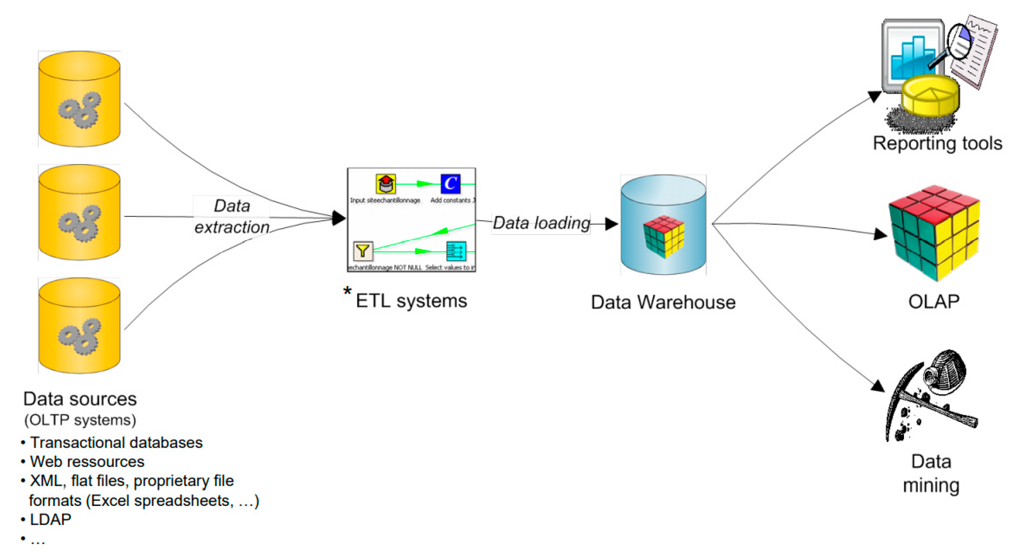
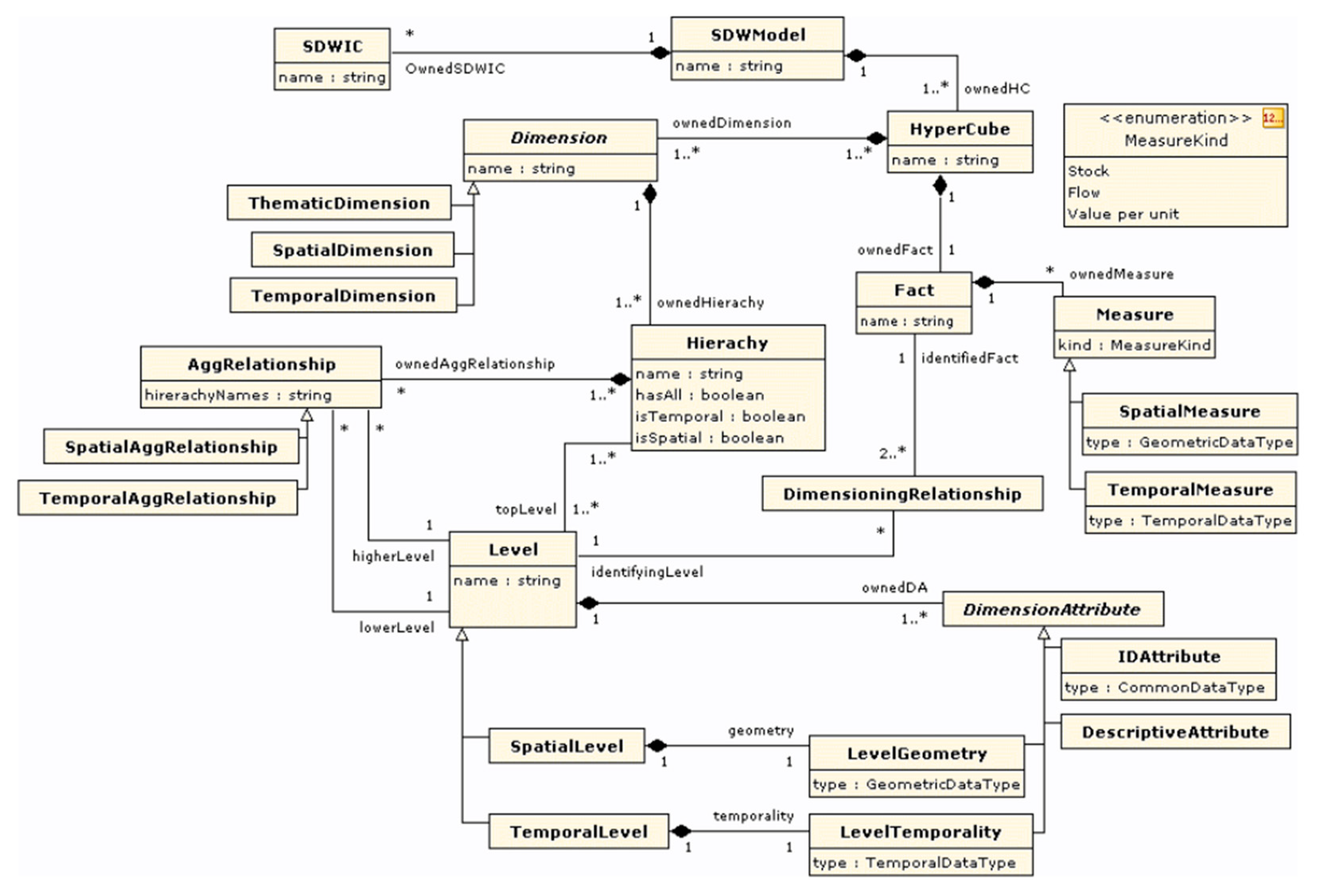
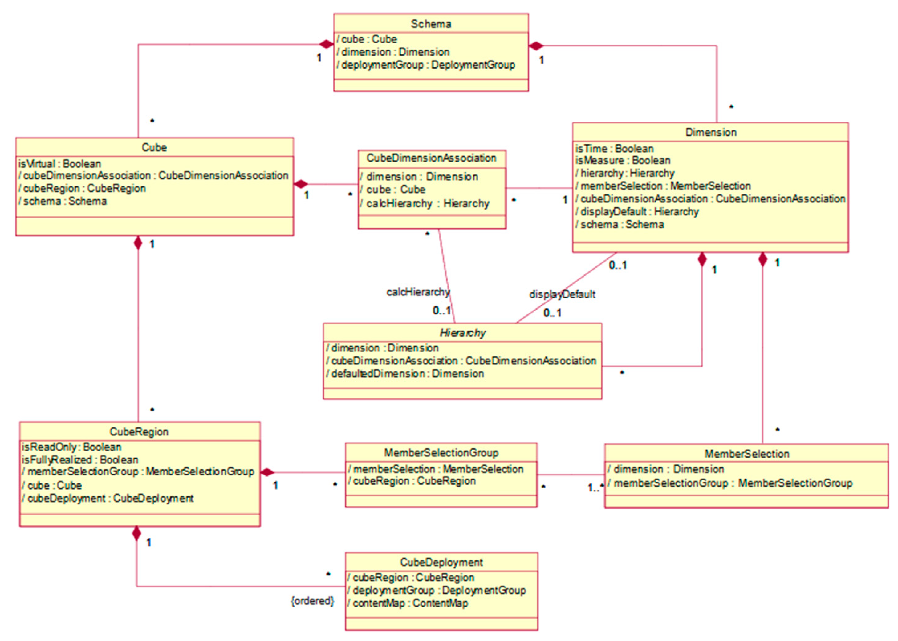
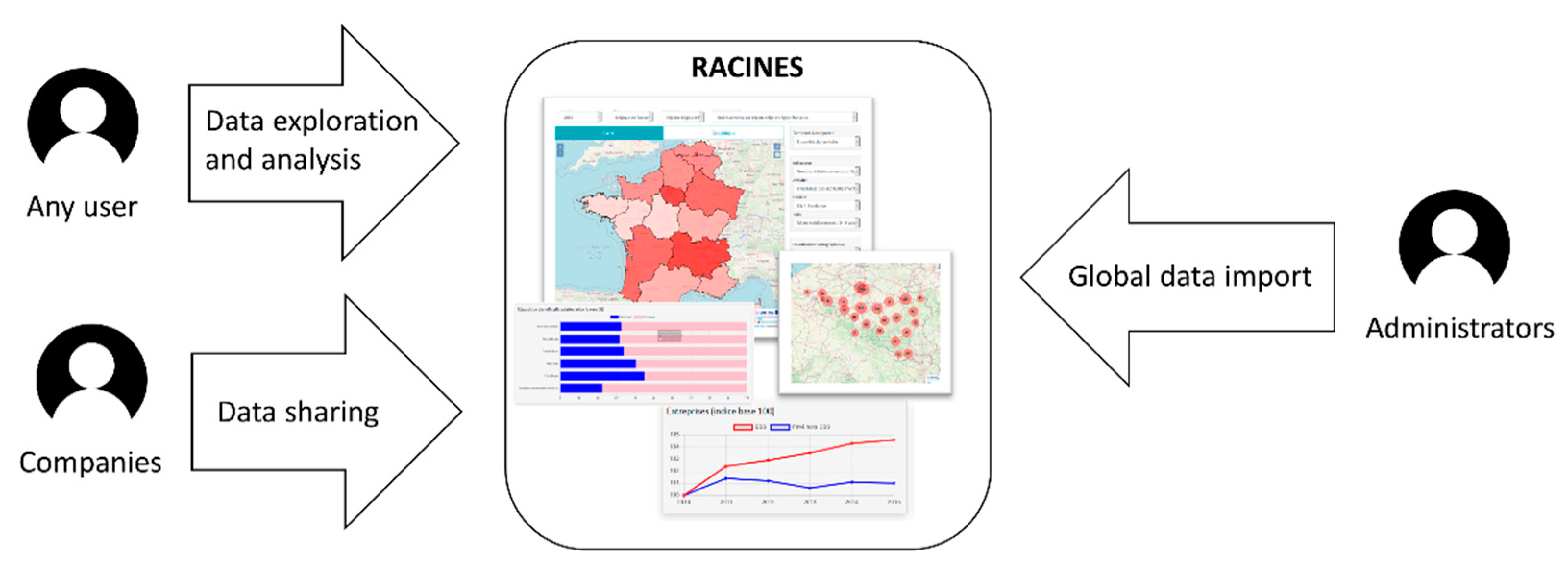
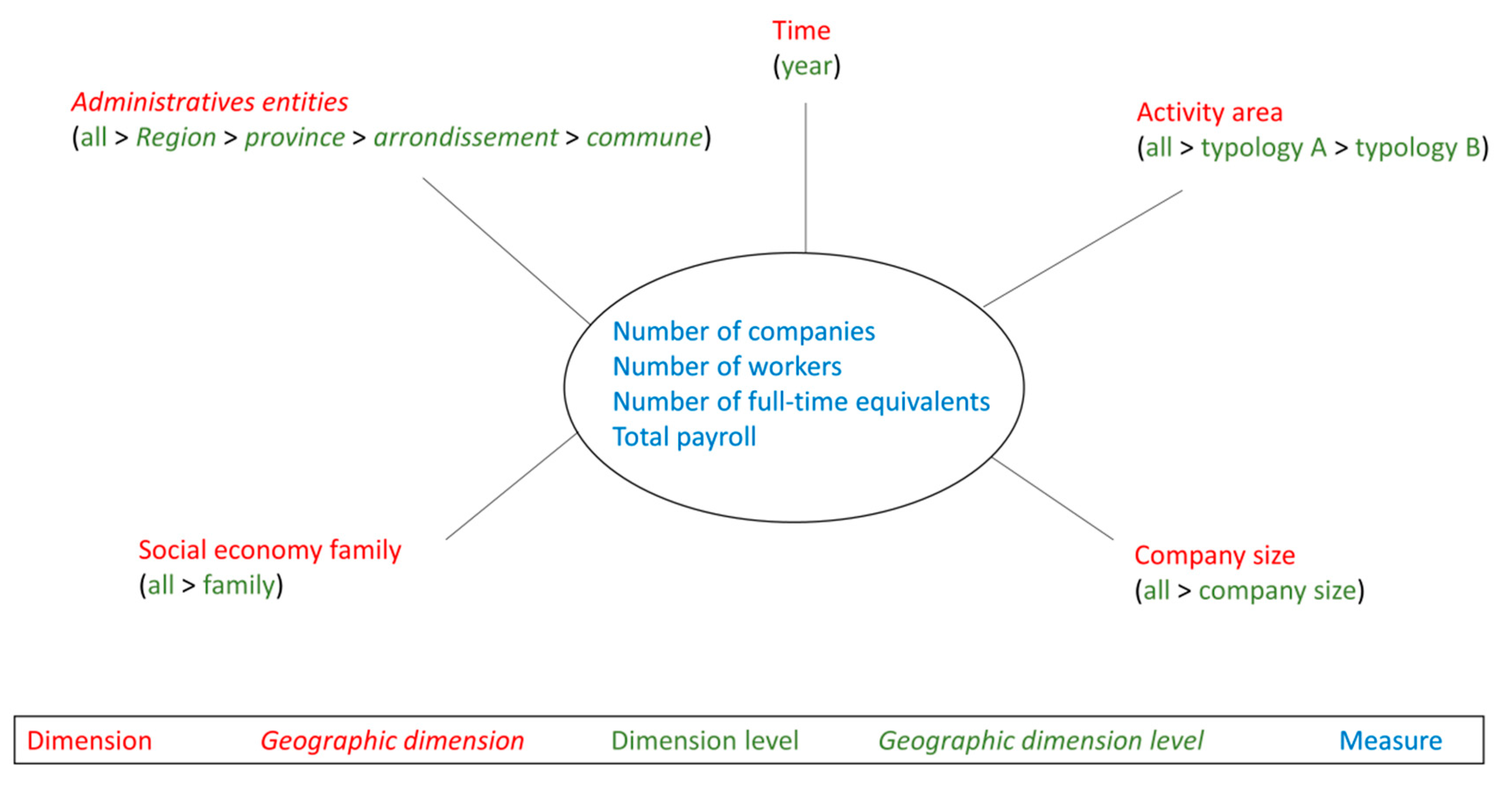
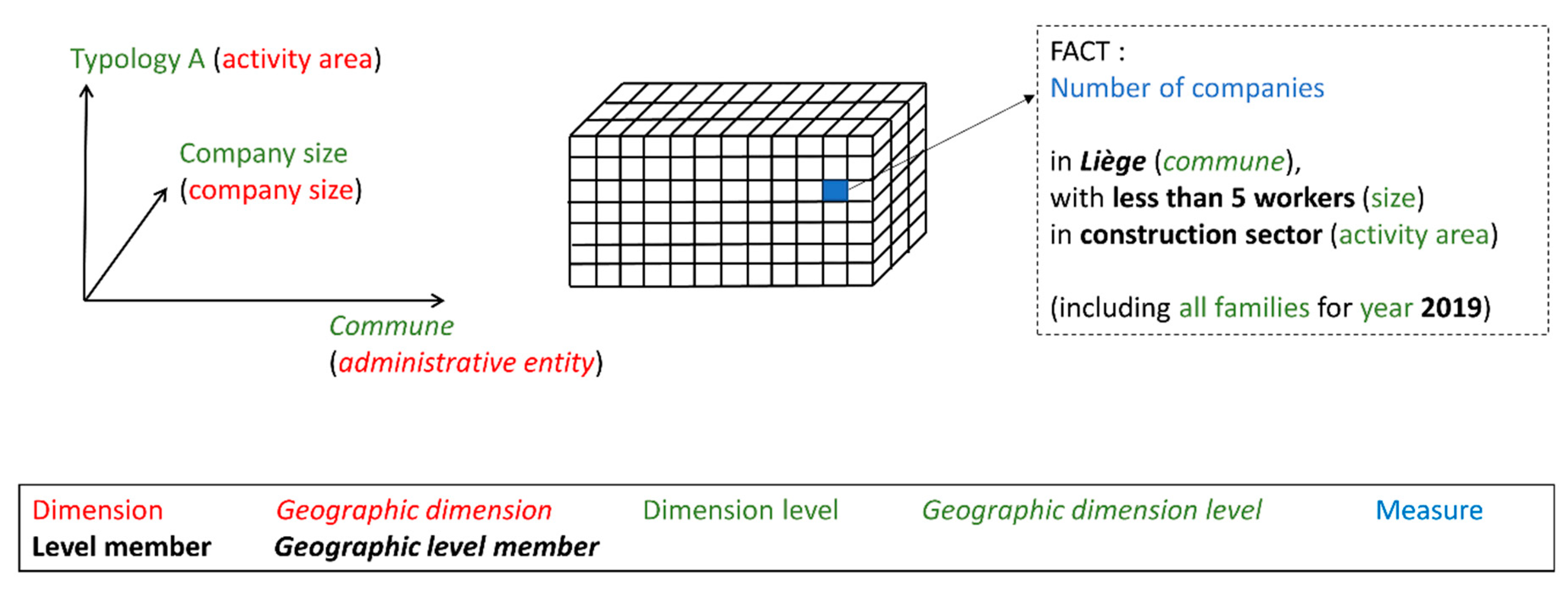
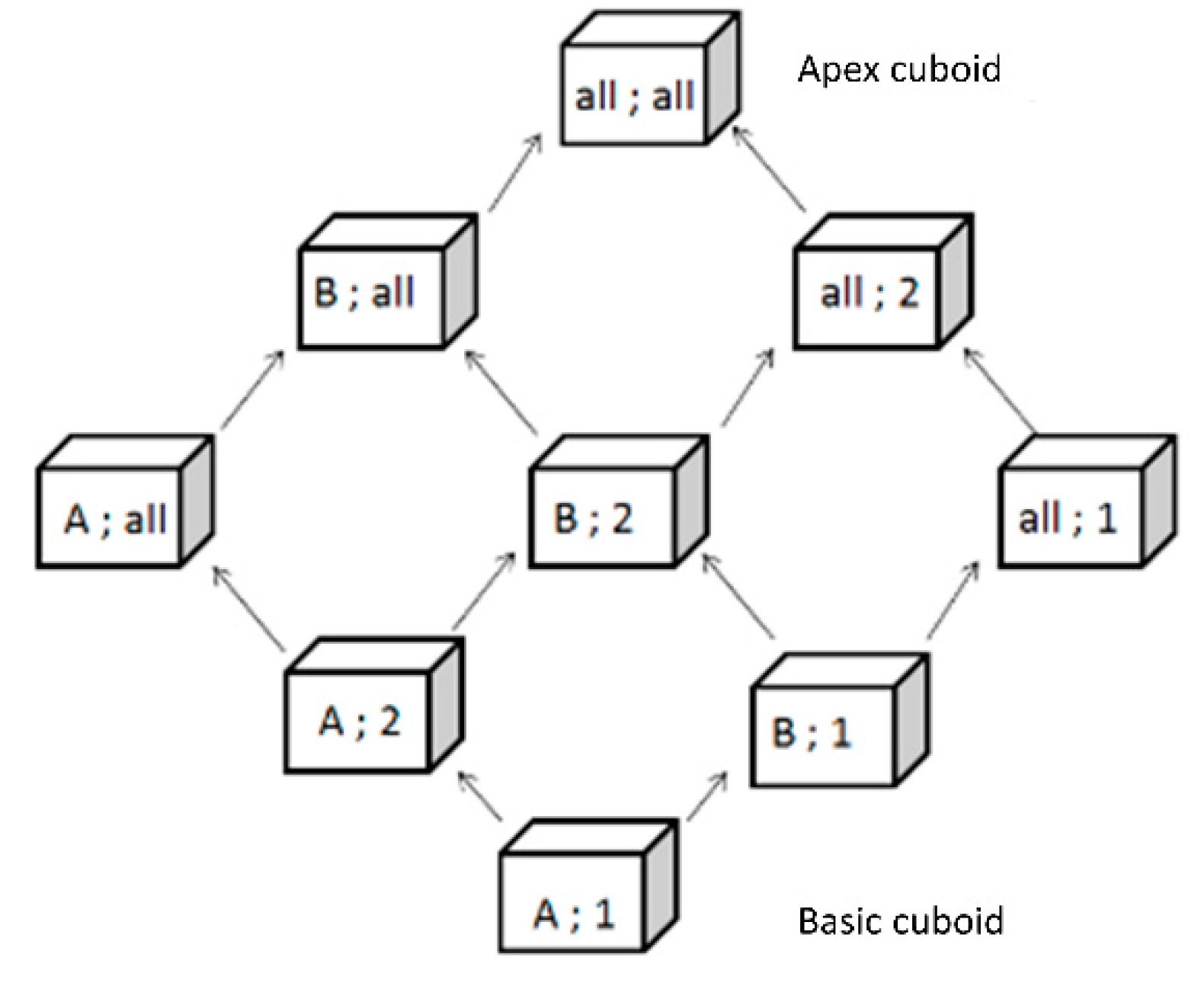
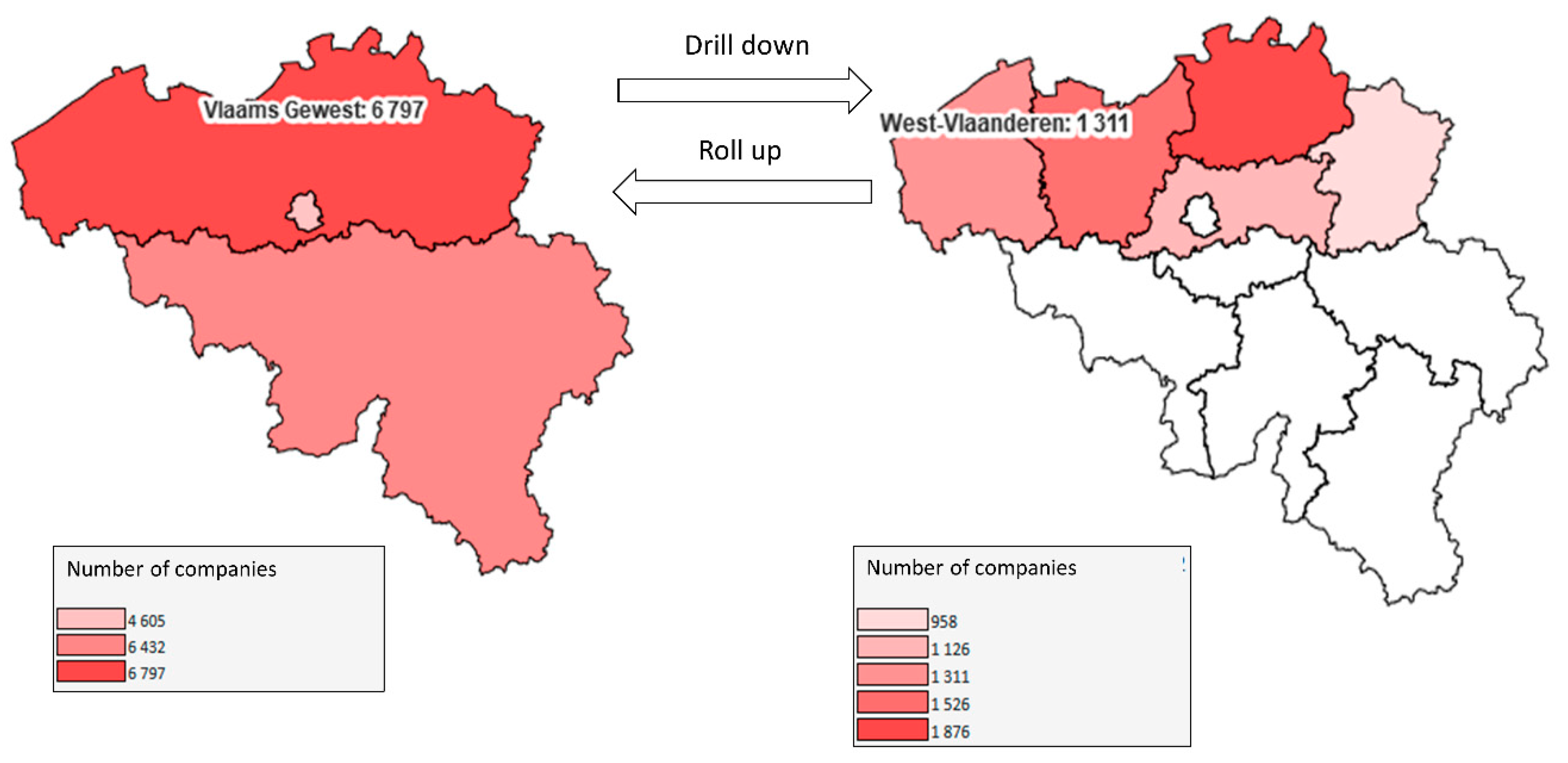
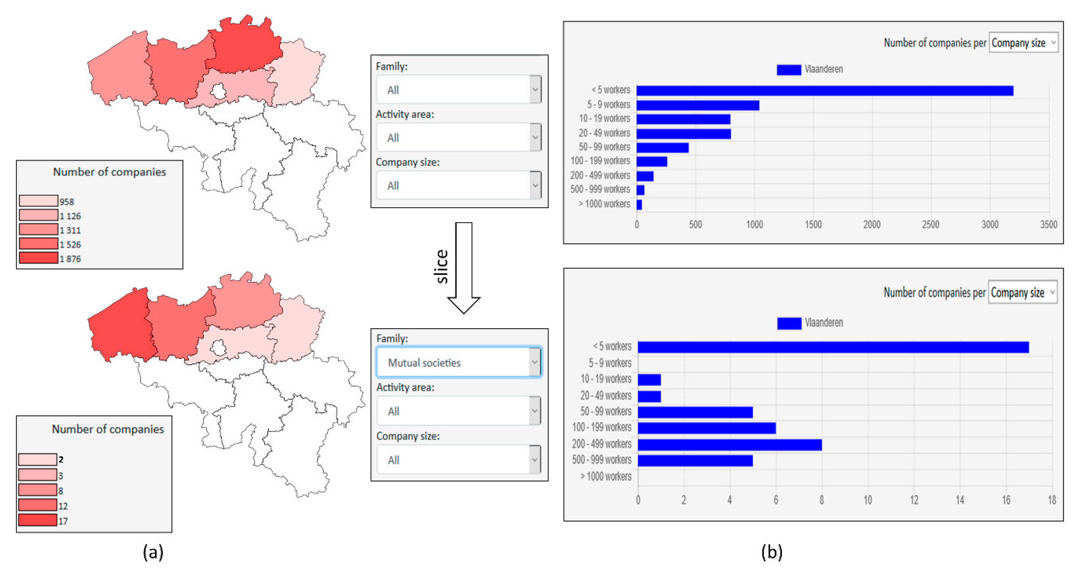
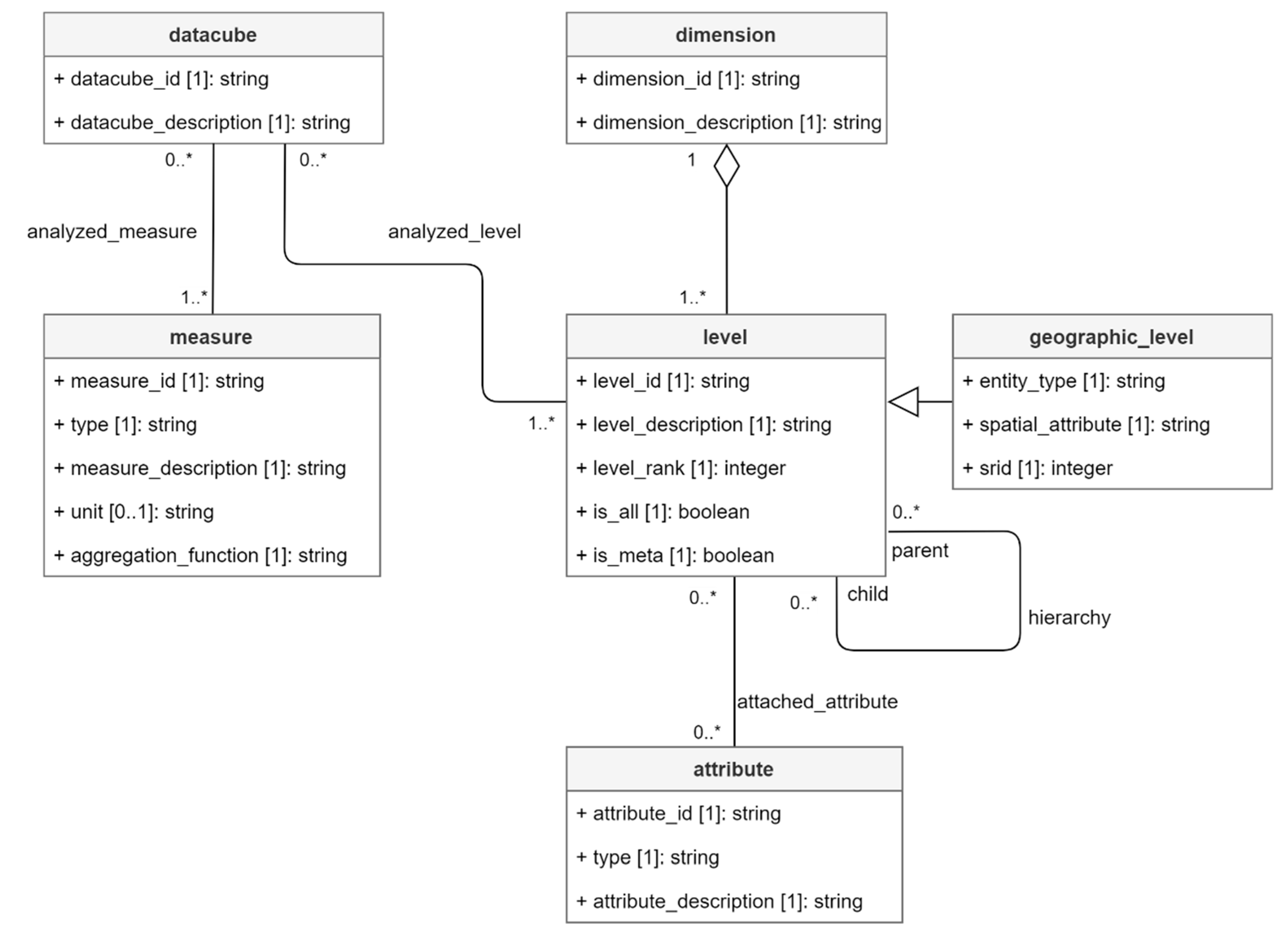
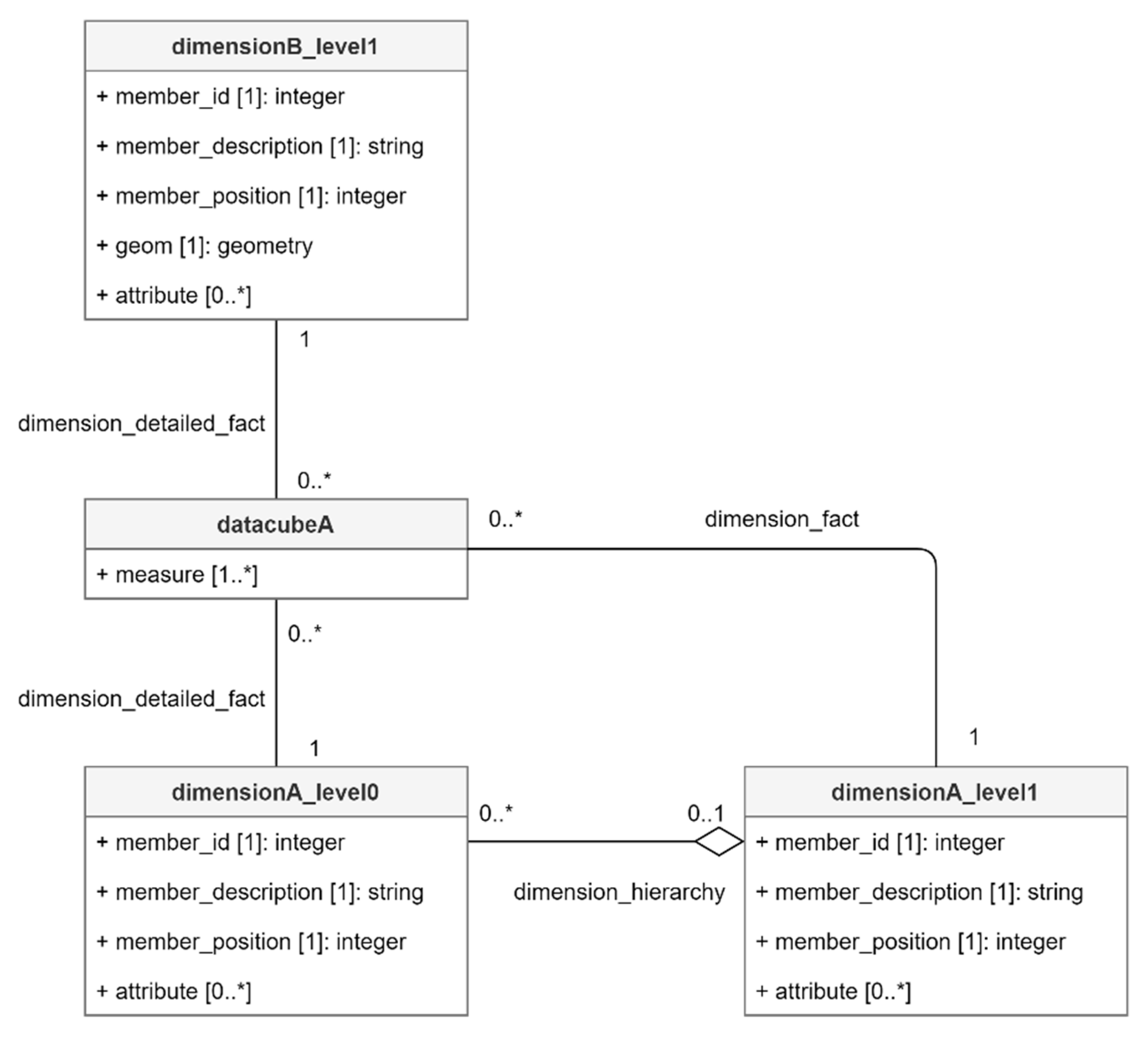
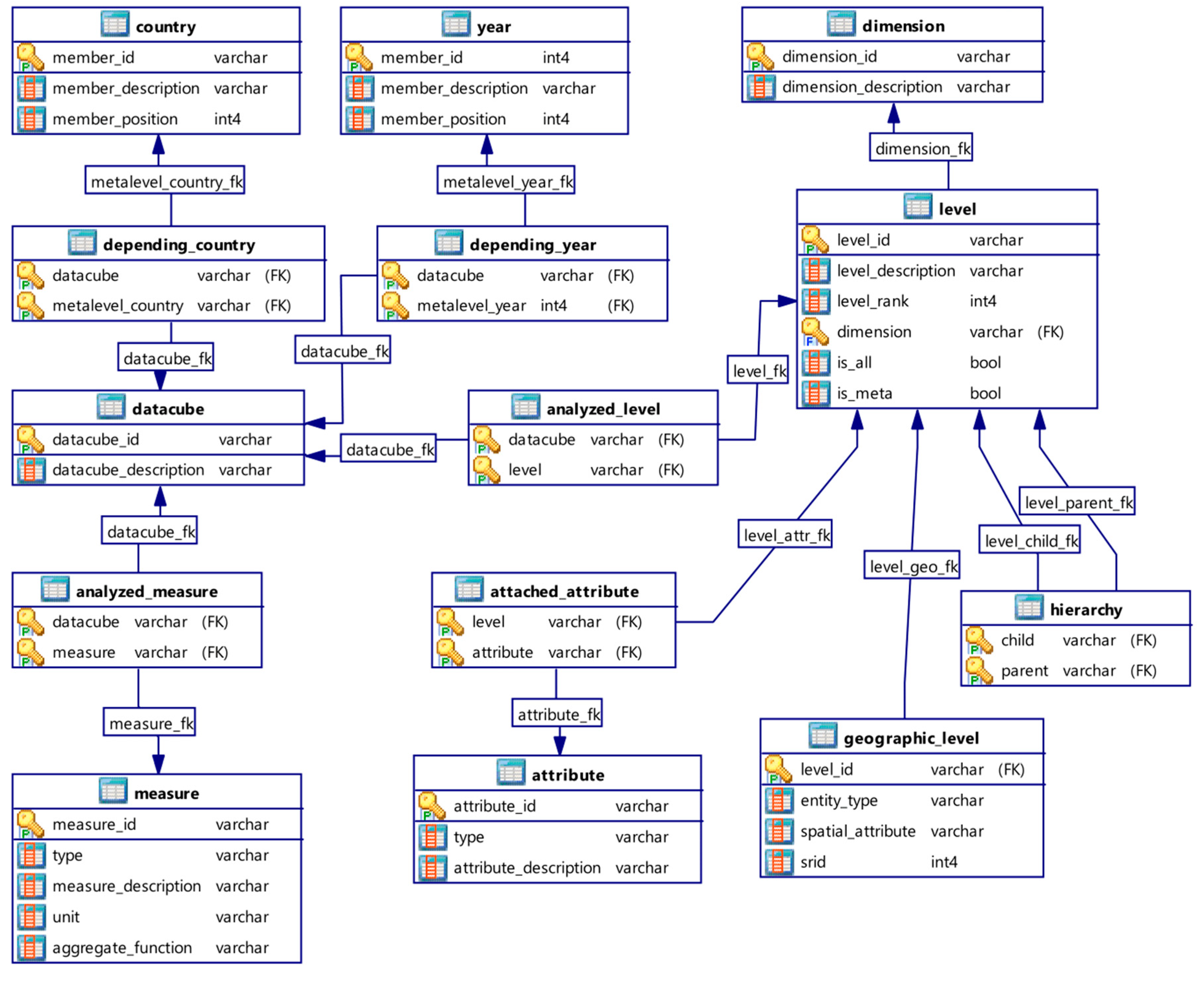
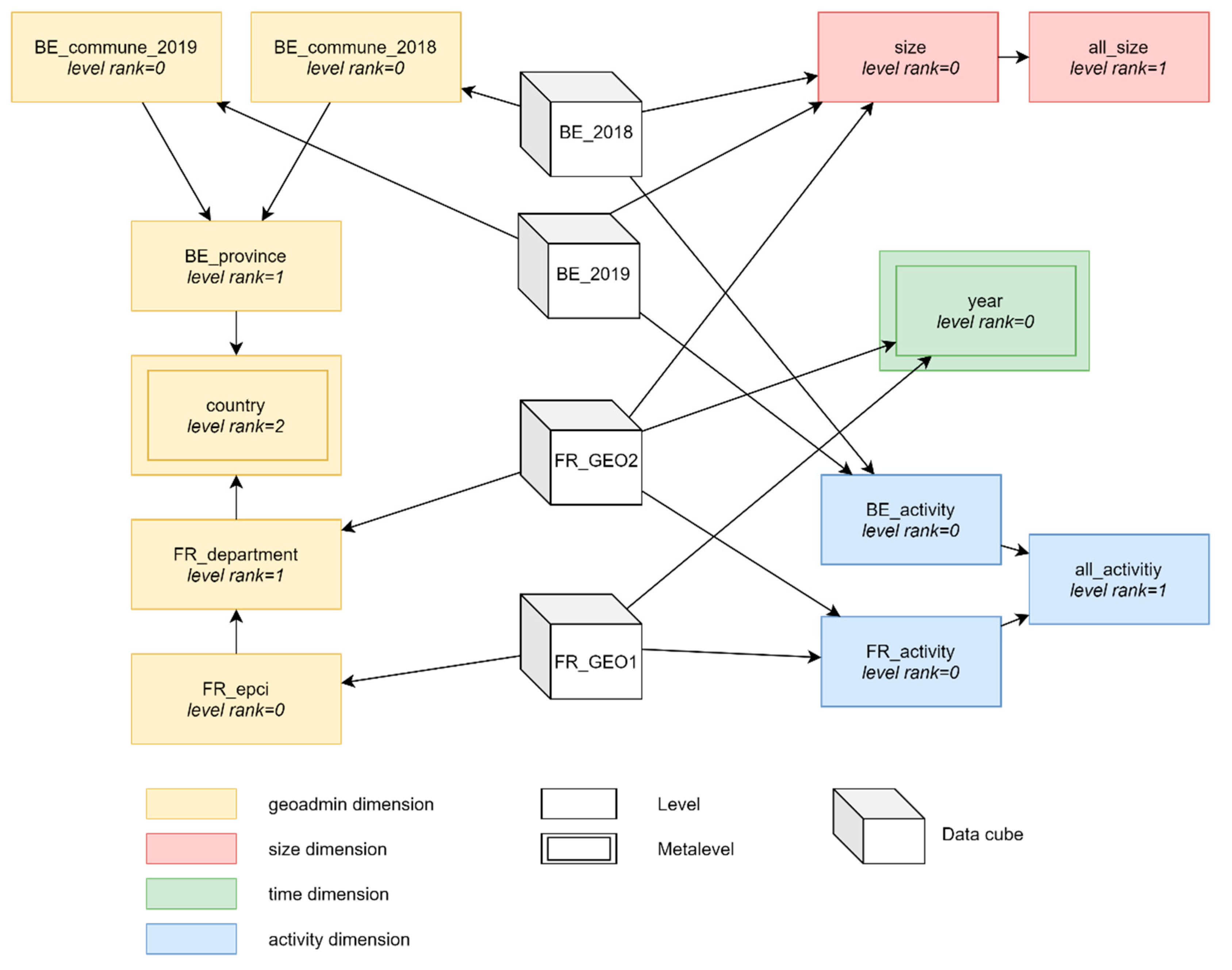
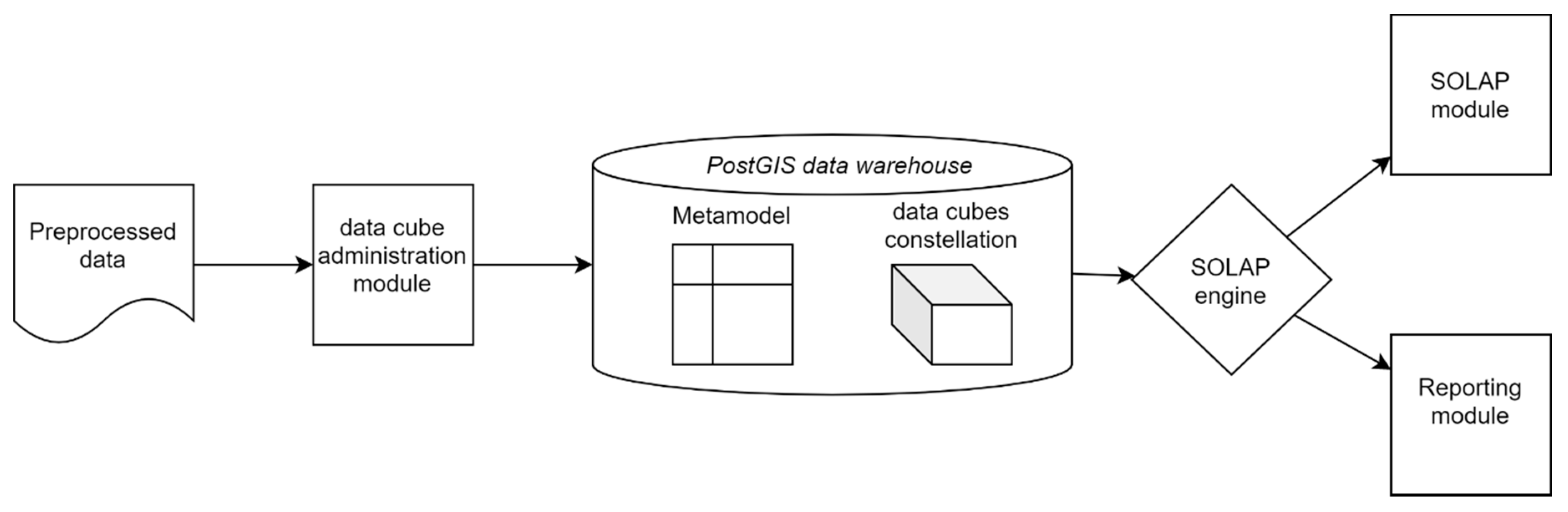
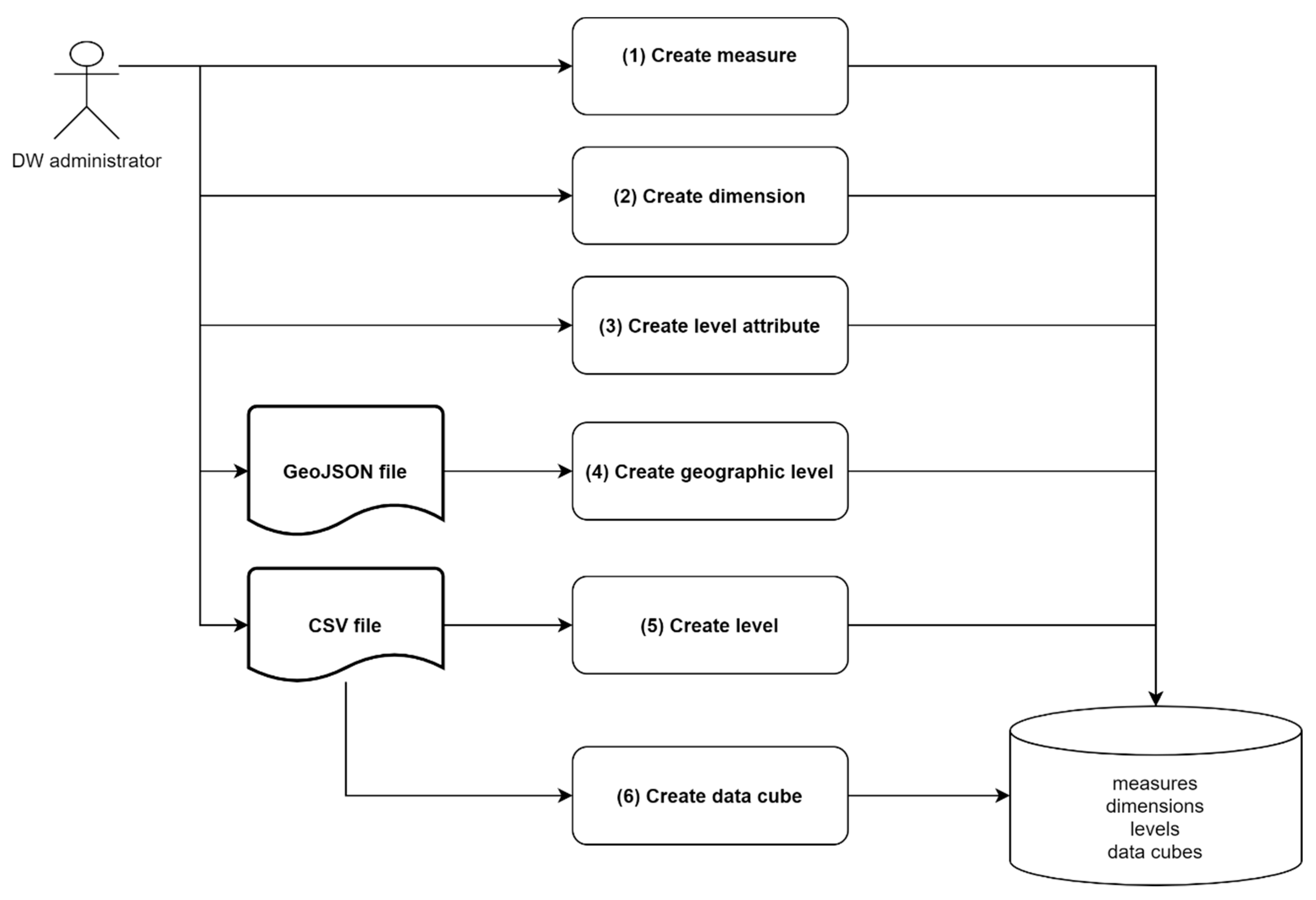
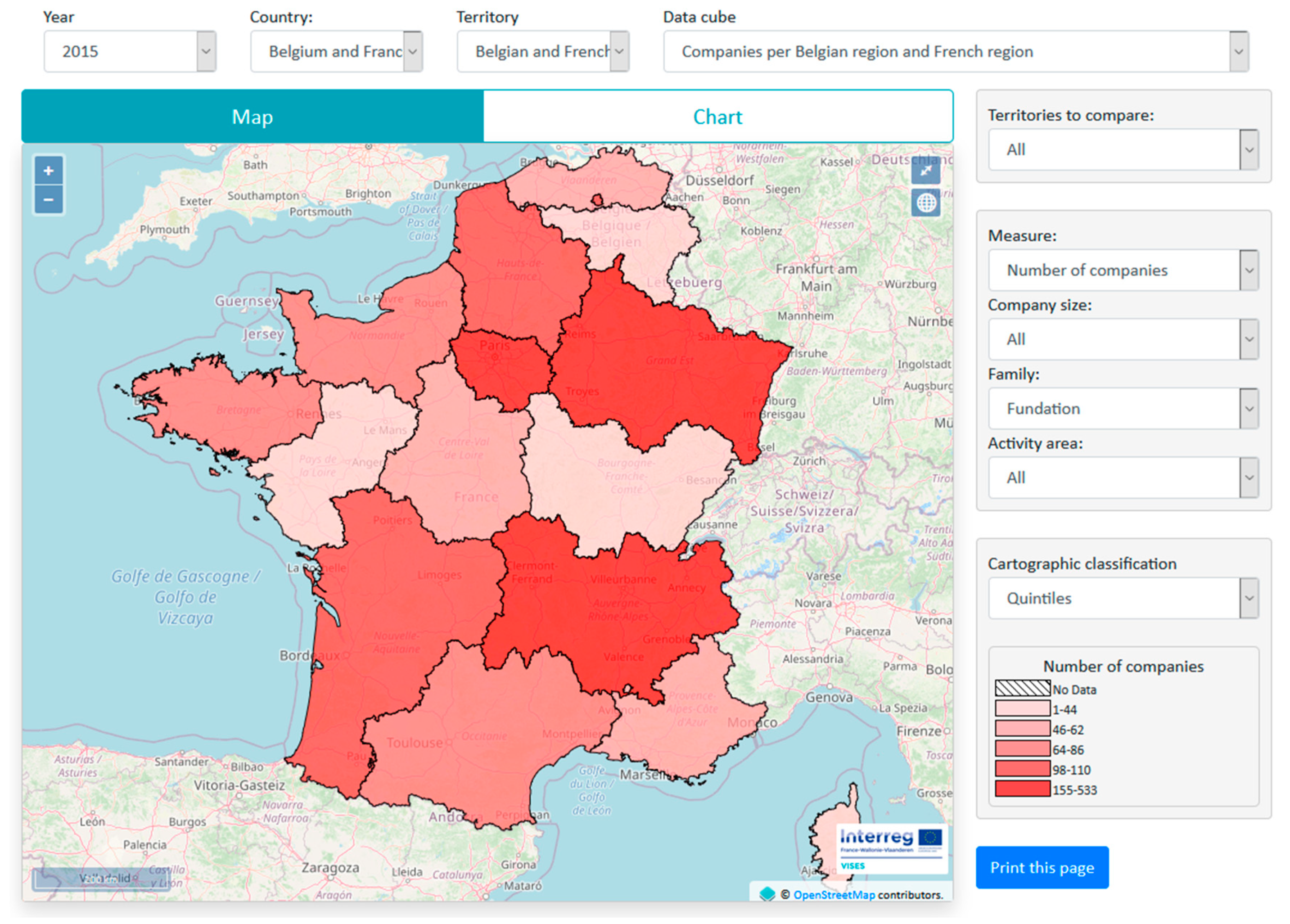
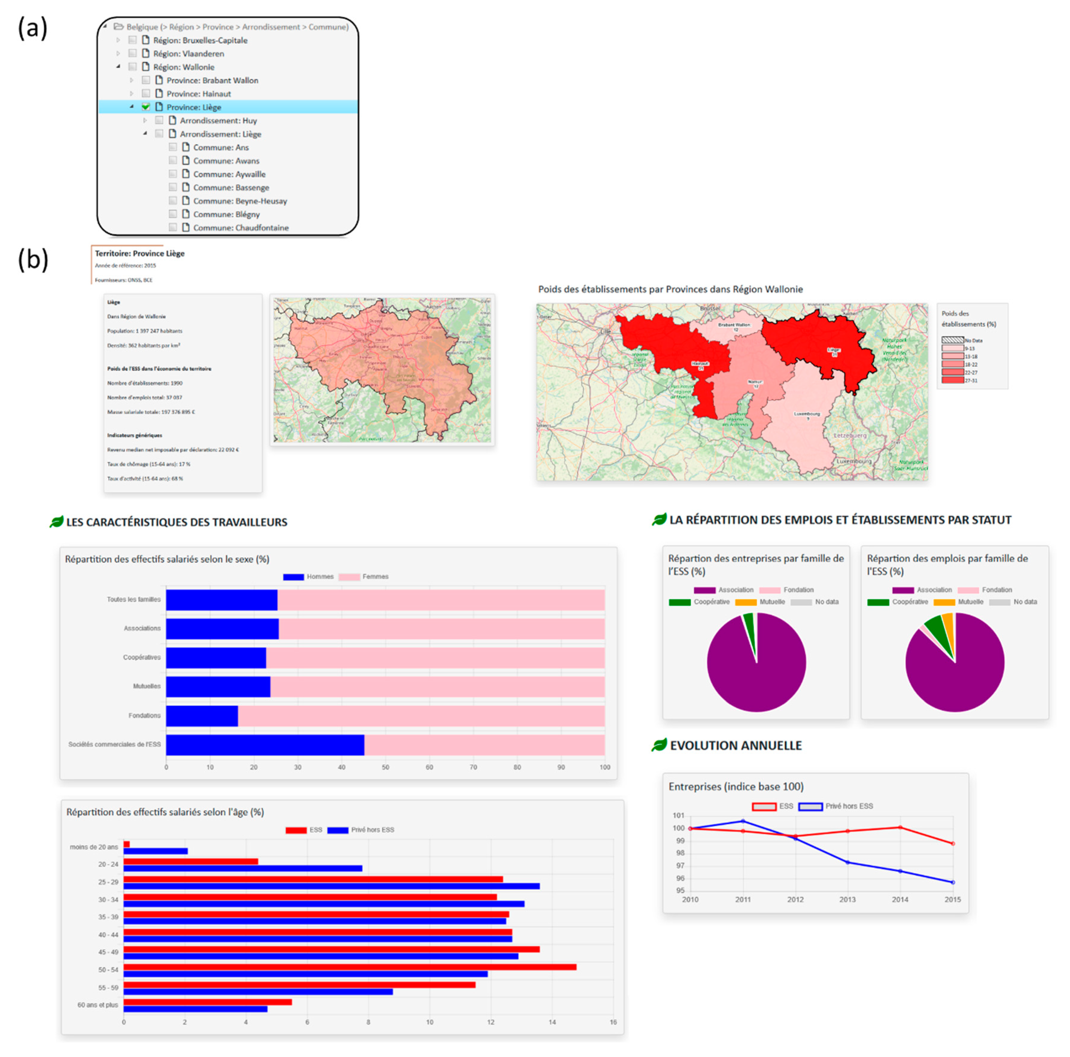
Table 1.
Data cube information given query 3.
| Dimension_id | Dimension_Description | Level_id | Level_Description | Level_Rank | Is_All |
|---|---|---|---|---|---|
| activity | Activity Area | fr_activity | French activity area | 0 | False |
| activity | Activity Area | all_activity | All activity areas | 1 | True |
| geoadmin | Administrative entity | fr_department | French Department | 1 | False |
| geoadmin | Administrative entity | country | Country | 2 | False |
| size | Company Size | size | Company Size | 0 | False |
| size | Company Size | all_size | All company sizes | 1 | True |
| time | Time | year | Year | 0 | False |
Publisher’s Note: MDPI stays neutral with regard to jurisdictional claims in published maps and institutional affiliations. |
© 2021 by the authors. Licensee MDPI, Basel, Switzerland. This article is an open access article distributed under the terms and conditions of the Creative Commons Attribution (CC BY) license (http://creativecommons.org/licenses/by/4.0/).
Share and Cite
MDPI and ACS Style
Kasprzyk, J.-P.; Devillet, G. A Data Cube Metamodel for Geographic Analysis Involving Heterogeneous Dimensions. ISPRS Int. J. Geo-Inf. 2021, 10, 87. https://doi.org/10.3390/ijgi10020087
AMA Style
Kasprzyk J-P, Devillet G. A Data Cube Metamodel for Geographic Analysis Involving Heterogeneous Dimensions. ISPRS International Journal of Geo-Information. 2021; 10(2):87. https://doi.org/10.3390/ijgi10020087
Chicago/Turabian StyleKasprzyk, Jean-Paul, and Guénaël Devillet. 2021. "A Data Cube Metamodel for Geographic Analysis Involving Heterogeneous Dimensions" ISPRS International Journal of Geo-Information 10, no. 2: 87. https://doi.org/10.3390/ijgi10020087
Note that from the first issue of 2016, this journal uses article numbers instead of page numbers. See further details here.