
Non-Stationary Modeling of Microlevel Road-Curve Crash Frequency with Geographically Weighted Regression


1
Lyles School of Civil Engineering, Purdue University, West Lafayette, IN 47907, USA
2
Division of Research and Development, Indiana Department of Transportation, West Lafayette, IN 47906, USA
*
Author to whom correspondence should be addressed.
ISPRS Int. J. Geo-Inf. 2021, 10(5), 286; https://doi.org/10.3390/ijgi10050286
Submission received: 13 March 2021
/
Revised: 22 April 2021
/
Accepted: 26 April 2021
/
Published: 30 April 2021
Abstract
:Vehicle crashes on roads are caused by many factors. However, the influence of these factors is not necessarily homogenous across locations, which is a challenge for non-stationary modeling approaches. To address this problem, this paper adopts two types of methods allowing parameters to fluctuate among observations, that is, the random parameter approach and the geographically weighted regression (GWR) approach. With road curvature, curve length, pavement friction, and traffic volume as independent variables, vehicle crash frequencies are modeled by two non-spatial methods, including the negative binomial (NB) model and random parameter negative binomial (RPNB), as well as three spatial methods (GWR approach). These models are calibrated in microlevel using a dataset of 9415 horizontal curve segments with a total length of 1545 kilometers for a period of three years (2016–2018) over the State of Indiana. The results revealed that the GWR approach can capture spatial heterogeneity and therefore significantly outperforms the conventional non-spatial approach. Based on the Akaike Information Criterion (AICc), geographically weighted negative binomial regression (GWNBR) was proved to be a superior approach for statewide microlevel crash analysis.
1. Introduction
Road horizontal curves are a critical factor for vehicle crashes due to their disproportional number of crashes. Traffic crashes cost over 30,000 lives in America every year. According to the Federal Highway Administration (FHWA) [1], more than 25% of fatal crashes are related to horizontal curves that occupy about 10% of the total system of mileage.
To reveal the intrinsic law of this phenomenon, several prediction models have been developed for curve crashes over the past decades. In terms of pavement condition, Buddhavarapu et al. [2] developed a crash injury severity model on two-lane horizontal curves in Texas. It was found that curve segments with smoother pavement are more likely to be high-risk, while longitudinal skid measurement shows little correlation with curve crash injury severity. To explore the influence of geometric features on curve crash frequency, a negative binomial model was developed by Schneider et al. [3] on the single-vehicle motorcycle crashes that occurred on curve segments of rural two-lane highways in Ohio. Geometric feature variables that significantly influence the motorcycle crash frequency were found to be curve radius, curve length, and curve shoulder width. Moreover, Musey and Park [4] presented a model for predicting horizontal curve crash severity with pavement friction and road curvature. The results demonstrated that serious injury occurs on curves with a higher degree of curvature, and lower friction is closely correlated to wet pavement crashes. Meanwhile, the correlation of crash frequency occurring at adjacent curves correlation is found to be significant by Gooch et al. [5].
All aforementioned models are global that assume parameter estimates are fixed across the geographical region of analysis. However, as location information is collected as a reference to crash data, some predicting variables may not be stationary. For example, the geometry features (such as radius and length) of horizontal curves may cause observation heterogeneity from unobserved factors such as various driver responses on curves, time-varying traffic, and weather conditions [6]. The effect of pavement friction may also vary across observations due to friction variations, a heterogeneous response in driver behavior, and climate influence. In terms of the effect of traffic volume on crash likelihood, there might also exist heterogeneous driver reactions to traffic as well as environmental factors [7]. Hence, modeling the relation between crash count and these explanatory variables with the overall fixed coefficient for the entire study area may cause biased estimates of the individual parameters. Thus, adding spatial variance with non-stationary models such as geographically weighted regression (GWR) and random parameter approaches may provide a better view for developing spatial dependency over space.
Traffic safety spatial studies are categorized as two levels of spatial aggregation: macrolevel and microlevel analysis. Conventionally, micro-level analysis focuses on specific road entities of the road network, such as intersections, rails, corridors, and road segments [3,8,9]. However, the macrolevel analysis focusing on zonal level crashes with various spatial units is becoming popular as part of the transportation planning process in recent research studies. The spatial units have been comprehensively developed recently, such as traffic analysis zones (TAZs) [10,11,12,13], counties [14,15], census tracts [16], wards [17,18], residential neighborhoods [19] and statistical area levels [20,21]. One of the advantages associated with macrolevel crash modeling is that it does not count on detailed data as much as microlevel crash models do [22]. However, it has been proved that the micro-level models with less detailed data still provide an acceptable accuracy when applying to non-stationary models [23]. It is, therefore, reasonable and promising to employ non-stationary models (i.e., geographically weighted regression and random parameter) for microlevel safety analysis.
2. Related Works
A number of road crash analysis methods have been developed to determine the spatial dependency and heterogeneity of parameter influence and to find out high-risk locations [24]. Among these methods, there was geographically weighted regression (GWR) [25], Bayesian models with conditional autoregressive [17], autoregressive models with spatial spillover effects [26], full Bayes multiple membership spatial model [27], and random parameter models [28].
GWR approach is the most promising technique to reveal the variables’ heterogenous effect over space in many fields (e.g., disease analysis [29], crime modeling [30]). Moreover, some highly scaled GWR tools (e.g., CUDA-based Parallel GWR [31] and FastGWR [32]) have been developed to process large volumes of data these years. We applied the GWR approach in this paper to address the issue that some variables have more impacts in certain spatial locations but fewer impacts in others. Moreover, the random parameter method is also utilized for comparison, as it also allows parameters varying from each other but has no spatial relationship involved. Since Fotheringham et al. [33] systematically illustrated GWR theory, this technique has often been applied to road safety analysis [34]. Hadayeghi et al. [25] explored GWR application to count data modeling for traffic safety analysis at the TAZ level. Li et al. [35] evaluated the performance of a geographically weighted Poisson regression (GWPR) model in comparison to a traditional generalized linear model (GLM) on county level crash data. Based on the semi-parametric GWPR model study of Nakaya et al. [36], where some variables may not significantly vary over space while others are spatially heterogeneous, Xu and Huang [28] examined the macrolevel crash data in Florida with random parameter negative binomial model (RPNB) and semi-parametric GWPR. Silva and Rodrigues [37] extended GWPR to model over-dispersed data by geographically weighted negative binomial regression (GWNBR) and geographically weighted negative binomial regression with global overdispersion parameters (GWNBRg). Gomes et al. [12] and Soroori et al. [13] applied GWNBR to model over-dispersed crashes for traffic zones, which outperformed GWPR and traditional global models. Amoh-Gyimah et al. [22] found that comparing with RPNB models and GLM models, the GWR approach provides better performance on macroscopic over-dispersed traffic crash frequency modeling. Nevertheless, only a few existing studies have investigated modeling state-wide microlevel regional safety on over-dispersed crash data. State-wide non-stationary crash frequency modeling involves coefficient variance on a larger number of observations and spacious areas. It is, therefore, necessary to study spatial heterogeneity of larger-scale crash data by the GWR approach.
The RPNB model, which also addresses unobserved heterogeneity in regional safety over-dispersed data modeling, assumes that the parameters draw from some random distributions and vary randomly from case to case. To investigate unobserved heterogeneity across highway segments for crash count prediction, Shaon et al. [38,39] and Chen et al. [40] applied random parameters Poisson-based models in their safety studies. As a branch of random parameter Poisson-based modeling, RPNB has been widely used to account for data overdispersion and has been widely conducted by Venkataraman et al. [6,41,42], Chen and Tarko [43], and Saeed et al. [44]. Xin et al. [45,46] have developed an RPNB model for Florida horizontal curves along two-lane, undivided highways motorcycle crashes with curve design factors. However, it is always a challenge to model spatial heterogeneity of large-scale over-dispersed crash count data and analyze their local differences.
Considering the fact that previous research studies were mostly conducted at the macro-level (zonal level), this paper explores different strategies for modeling local variation of over-dispersed crash count data in state-wide highway horizontal curves with relation to curve segment characteristics at a microlevel (each observation). The paper is organized as follows: Section 2 introduces the methodologies used in this paper, while Section 3 describes data preparation. Section 4 presents the estimation results, compares results from different models, and interprets the results locally. Section 5 summarizes the findings of our work and recommends future efforts.
3. Methodologies
This section presents the general forms of the five models of two types to be used in this paper: negative binomial (NB), RPNB; GWPR, GWNBR, and GWNBRg. We also provide a brief description of the estimation procedures. These models are discussed in two groups: non-spatial models and spatial models (GWR approach). The section starts with a description of two non-spatial methods: the traditional NB regressions and the RPNB model. The other three GWR types of models, that is, GWPR, GWNBR, and GWNBRg, are calibrated as spatial regression. At last, a brief illustration of the goodness of fit measures is presented.
3.1. Non-Spatial Models
For non-negative integer crash count data, Poisson regression is the most basic one [47]. However, the property of Poisson distribution that variance is identical to the mean is often violated in crash count data [48]. NB regression model has been generally applied to account for the issue of over-dispersion. NB regression model can be presented using log-linear function while the Poisson parameter () is composed of systematic terms and a random term as following:
where is the expected number of crashes in observation , , are the model parameters, is the th explanatory variable for observation , is the number of model parameters, is a gamma-distributed error term with mean 1 and variance . The addition of the gamma-distributed error term allows the variance of the dependent variable to differ from its mean such that . When α approaches zero, negative binomial regression is the same as Poisson regression. The negative binomial regression is appropriate when significantly differs from zero [49].
NB model can depict the over-dispersion character of traffic crash data; however, possible spatial dependency among curve segments may be ignored, as stated before. By incorporating a random term into the NB model function, that is, Equation (2), an RPNB model can be employed in response to the non-stationary explanatory variables in count models:
where is the parameter of the th explanatory variable for observation , is the mean parameter across all observation, and is a randomly distributed term with an analyst-specified distribution (like normal distribution with mean 0 and variance ) that describes unobserved heterogeneity. If some of the variances of the distribution are tested as not significantly different from zero for an individual explanatory variable, the conventional fixed-parameter across all observations is statistically appropriate. If the constant term is the only random parameter, a random parameter model is equivalent to a random effect model.
In most cases, observations are structured to groups to capture heterogeneity among groups for random parameter models, and can be rewritten as , where is a random term that describes unobserved heterogeneity across analyst-specified groups regarding the th explanatory variable [7]. Namely, an analyst-specified group shares the same random term for explanatory variables.
3.2. Spatial Models
To deal with spatial non-stationarity, the GWR approach is considered in this paper. The basic model to interpret spatial heterogeneity problems is the GWPR model developed by Nakaya et al. [36], which allows estimated regression parameters to vary over space. The following framework forms the model:
where the estimated coefficients are determined by location = denoting curve segment midpoint coordinates, and implies that the parameter varies among curve segments.
The parameters matrix for each spatial unit are estimated as follows:
where is local regression coefficients for the spatial unit , X is the design matrix of explanatory variables, is the transposed X, Y is dependent variables, and denotes an spatial weighting matrix which is defined as:
where is the geographical weight of the th observation at the th regression point. In GWR approach theory, estimating the parameters of each regression point is based on the other observations within an appropriate bandwidth. These nearby observations are assigned weight according to the distance from observations to the regression point in the regression process. For each regression point, observations locating from the edge of the bandwidth to the egression point would yield more weight. The weight is commonly calculated by two types of conventional kernels, that is, the Gaussian and the bi-square (adaptive) functions defined as follows:
where is the distance between neighbor observations and , is the fixed bandwidth, and is an adaptive bandwidth size defined by the k-th nearest neighbor distance [50]. The bandwidth is constant in the Gaussian function (fixed kernel), while the bandwidth of the adaptive bi-square function varies in response to sample location density.
The Corrected Akaike Information Criterion (AICc), AIC with a correction for small sample sizes, is applied to select optimum bandwidth and model comparison illustrated in the next section. The lower AICc a model can generate, the better performance it provides [25,36,50].
Similar to traditional count models, the violation of the Poisson distribution also happens when variance differs from the mean. The negative binomial form is also applied to the GWR approach to account for the overdispersion problem. Silva and Rodrigues [37] developed an algorithm to model over-dispersed data in a non-stationary way by GWNBR. The proposed GWNBR model is defined as:
where the gamma-distributed error term is the same with Equation (1), but only varies over spatial units. The other terms are as defined in Equation (4). A modified Iteratively Reweighted Least Squares (IRLS) procedure is used to estimate the parameters and α. Applying the Newton-Raphson (NR) algorithm, a subroutine with the maximum likelihood (ML) method can be carried out in this procedure. (Silva and Rodrigues, 2014).
Set the predicted mean as , parameterizing this model in terms of , gives the offset variables. Thus, this model can be expressed as or . The parameter vector for each spatial unit is determined by:
where is an nn GLM diagonal weighting matrix for iteration m and location , are adjusted dependent variables. The other terms are as defined earlier in the GWPR model. The effective number of parameters of the GWNBR can be calculated by adding effective numbers of parameter in response to and .
To simplify the calculation of GWNBR, GWNBRg introduces a global overdispersion parameter. It can be noted as or , where the parameters are the same as in GWNBR. The estimation of the overdispersion parameter in GWNBRg is the same as that obtained from the non-spatial negative binomial model. Because of no spatial variation for α, the effective number of the parameters contributed from equals 1.
3.3. Measures of Goodness of Fit
To provide the average magnitude of the variability of prediction, the median absolute deviation (MAD) is employed:
where is the number of observations (i.e., the number of curve segments in this paper), and is the predicted crash frequency and is the observed crash frequency. The smallest value of MAD is the best result in prediction.
Another goodness of fit measure— is also adopted to consider the model complexity as follows:
where represents the deviance, is the number of parameters estimated in the model, is the number of observations. The deviance of the Poisson regression model can be expressed as:
With regard to spatial regression estimation, the number of parameters is replaced to the effective number of parameters, which can be defined as (Fotheringham et al. 2002):
where matrix S is computed by [36]:
4. Data Description
We use crash data in the state of Indiana in the US to evaluate the performance of different models. The data include US and State Highways in Indiana from 2016 to 2018. They were retrieved from the Automated Reporting Information Exchange System (ARIES) portal (https://www.ariesportal.com/, accessed on 26 April 2021). As there are errors in GPS coordinates recorded by police officers [51], we applied the CLIP software developed by the Center for Road Safety [52] to correct crash occurrence location by geocoding position description for each crash record. It is not perfect to apply three years of crash data but the data used in this paper include around 7000 crashes, which is sufficient for a traffic safety study.
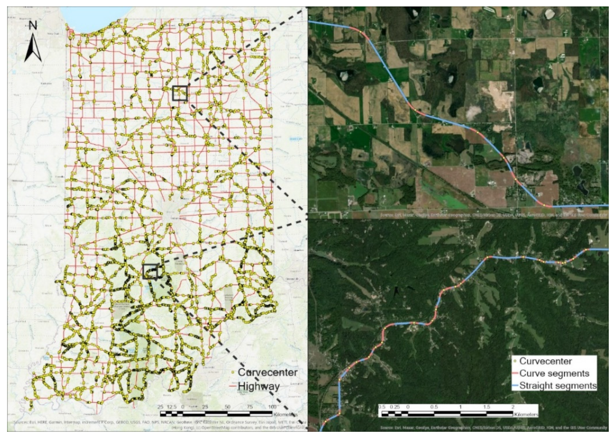
The horizontal curve segments are generated as the primary data. To do so, the road network database provided by FHWA Highway Performance Monitoring System (https://maps.indiana.edu/layerGallery.html?category=Streets, accessed on 26 April 2021) was used to detect and extract horizontal curve segments by ROCA (ROad Curvature Analyst) [53] tool in ESRI ArcGIS. Figure 1 shows state-wide curve segment distribution and two typical road curve identification examples at the plain area and mountain area. Out of a total 17,381 km road network for Indiana State Route and US Highway, 1545 km curve segments were identified and adopted as the base units. Four independent variables were selected for crash count modeling. Among them, the radius and length of curves are calculated by the ROCA software as geometric variables. Although curve radius and curve length are designed by a certain correlation in the planning process. In this paper, curve segments are identified from the road network shapefile, meaning that the length of a curve segment is not correlated with its radius (correlation efficiency between them is 0.337).
The third independent variable is pavement friction. Pavement friction data measured at 40 mph with standard smooth tires were retrieved from the network pavement friction database of the Indiana Department of Transportation (INDOT). The AADT (Annual Average Daily Traffic) was selected as the fourth independent parameter. The AADT shapefiles from 2016 to 2018 were downloaded from the INDOT traffic flow website (https://www.in.gov/indot/2469.htm, accessed on 26 April 2021), where road sections that have relatively uniform travel characteristics are assigned the same value.
Crashes were filtered with a horizontal curve segment 50 m buffer. Crash counts are summed for three years of crash frequency for each curve segment. Curve segments were aggregated with the nearest pavement friction shapefile and AADT shapefile by ArcGIS.
The variables used for model specification and their descriptive statistics are summarized in Table 1. Because of a closer linear relationship with the dependent variable being observed on the logarithmic scale, the logarithmic transformation is applied to the independent variable in this research. The Variance Inflation Factor (VIF) is employed to assess multicollinearity among variables in this data. The VIF’s of all the variables have values lower than two, indicating that there is no significant multicollinearity [54]
5. Results and Discussion
Curve crash frequencies at the microlevel were estimated by the representatives of spatial (GWPR, GWNBR, and GWNBRg) and non-spatial (NB, RPNB) models using the dataset described in Section 4. The estimation of the RPNB model and GWR approach were performed by NLOGIT6 and Golden macro in SAS®9.4 [55], respectively.
5.1. Model Comparison
For the GWR approach, a fixed Gaussian function is applied as kernel function curve segments were identified from the road network. Assuming that the unobserved heterogeneity of curve crashes comes from climate, terrain, and driver behavior, their spatial correlation matrix should be independent of the number of neighbors. Thus, the bandwidth is set to be Gaussian fixed kernel functions as defined in Equation (7), and the distance between a pair of curve segments midpoint is set as Euclidean distance in the kernel function. Moreover, the optimum bandwidths with the lowest AICc for the GWR approach were selected by SAS Golden macro.
We estimate the RPNB model by using the normal distribution as a parameter density function. It is worked out by 100 Halton plots simulation-based maximum likelihood. This model is applied to account for heterogeneity among individual curve segments to compare with the GWR approach that assumes parameters varying among curve segments. Although specifying groups in the random parameter model are popular, as mentioned in Section 3.1, there is no need to divide the data into groups in this research.
The results of the model estimations are presented in Table 2. Several general observations are worth noting. GWNBR performs best with the lowest value of AICc and the highest value of log likelihood, indicating that by accounting for the spatial heterogeneity of all variables and dispersion parameters, curve crash frequency is depicted best by the GWNBR model. Concerning the MAD metric, GWPR surprisingly observed a smaller MAD value than GWNBR models. One explanation of this result is that the GWPR model with the smallest MAD tends to have a bandwidth much smaller than the GWNBR model’s. Smaller bandwidth size allows GWPR to depict local varying parameters and makes it less vulnerable for extreme values. Furthermore, RPNB and GWNBRg have similar performance for log likelihood and AICc, where both assume that the dispersion parameter does not vary over space. Finally, the traditional NB model expectedly performs worst for every goodness of fit measure.
To quantify the spatial autocorrelation of the predicted residuals for these models over curve segments, Moran Global Index (I) [56] is employed. Moran’s I value varies between -1 to 1, where 0 indicates a perfect random spatial distribution. A positive value implies similarity among the neighbors and residual are concentrated, while a negative value means discrepancy among neighbors and residuals are dispersed. In summary, the higher the absolute value Moran’s I is, the stronger the spatial autocorrelation data has. The results are presented in Table 2.
Moran’s I result shows that NB has the highest value, reflecting that relatively high spatial autocorrelation without considering spatial variation. GWPR, GWNBR, and GWNBRg show decreasing Moran’s I values but all smaller than those from NB and RPNB, which may be related to their different optimum bandwidth (GWPR < GWNBR < GWBNRg). Namely, local patterns depicting from the model can strongly reduce residual prediction autocorrelation. However, none of these models shows significance on the non-autocorrelation of prediction residuals. From Table 2, the reduction of residual autocorrelation from NB to GWNBR models shows 99% significance, indicating that GWNBR is possible to produce a relatively non-biased estimation comparing to the global model.
5.2. Statistics of Estimated Parameters
Estimated parameters are summarized in Table 3. Parameters are denoted as LOGR, LOGL, LOGF, and LOGA, representing the logarithms of radius, length, friction, and AADT, respectively. The local parameters in RPNB and GWR approach were described by the minimum, lower quartile, median, upper quartile, and maximum of values, while only point estimation of coefficients in the NB model is provided. The parameters of global NB show positive signs for curve length and traffic volume (LOGL and LOGA), which represents that crash frequency rises with the increase of curve segment length and traffic count. The estimations of the curve radius and pavement friction (LOGR and LOGF) have shown negative global parameters, which do make sense and agree well with the recent research findings [57,58]. As shown in Table 3 and Table 4, the parameter statistics reveal that: (1) Mean and median values of estimated parameters generated from all these non-stationary models are close to that obtained from the global negative binomial model, indicating that the global model generally reflects the average impact of these factors in non-stationary models. (2) The range of var ying parameters can be ranked as GWPR > GWNBR > GWNBRg > RPNB, which accords with the discussion in the next section.
It is also worth noting that there exist counterintuitive signs in GWPR and GWNBR. The GWPR model had counterintuitive signs of coefficients for some observations for the regression intercept and the LOGR, LOGF, and LOGA. The GWNBR model also had some counterintuitive signs of coefficients for the LOGR. Since the spatial coefficient multicollinearity has been proved to be not responsible for the counterintuitive signs [59], this result can be explained by the hypothesis that some variables may not be significant in certain areas. These local areas may have insignificant counterintuitive signs for some variables [12]. This can be confirmed by observing the coefficient spatial distribution of the GWPR and GWNBR in Figure 2. Unexpected significant counterintuitive signs among variables in GWPR might be caused by the failure considering data overdispersion [28].
5.3. Spatial Heterogeneity of Estimated Parameters
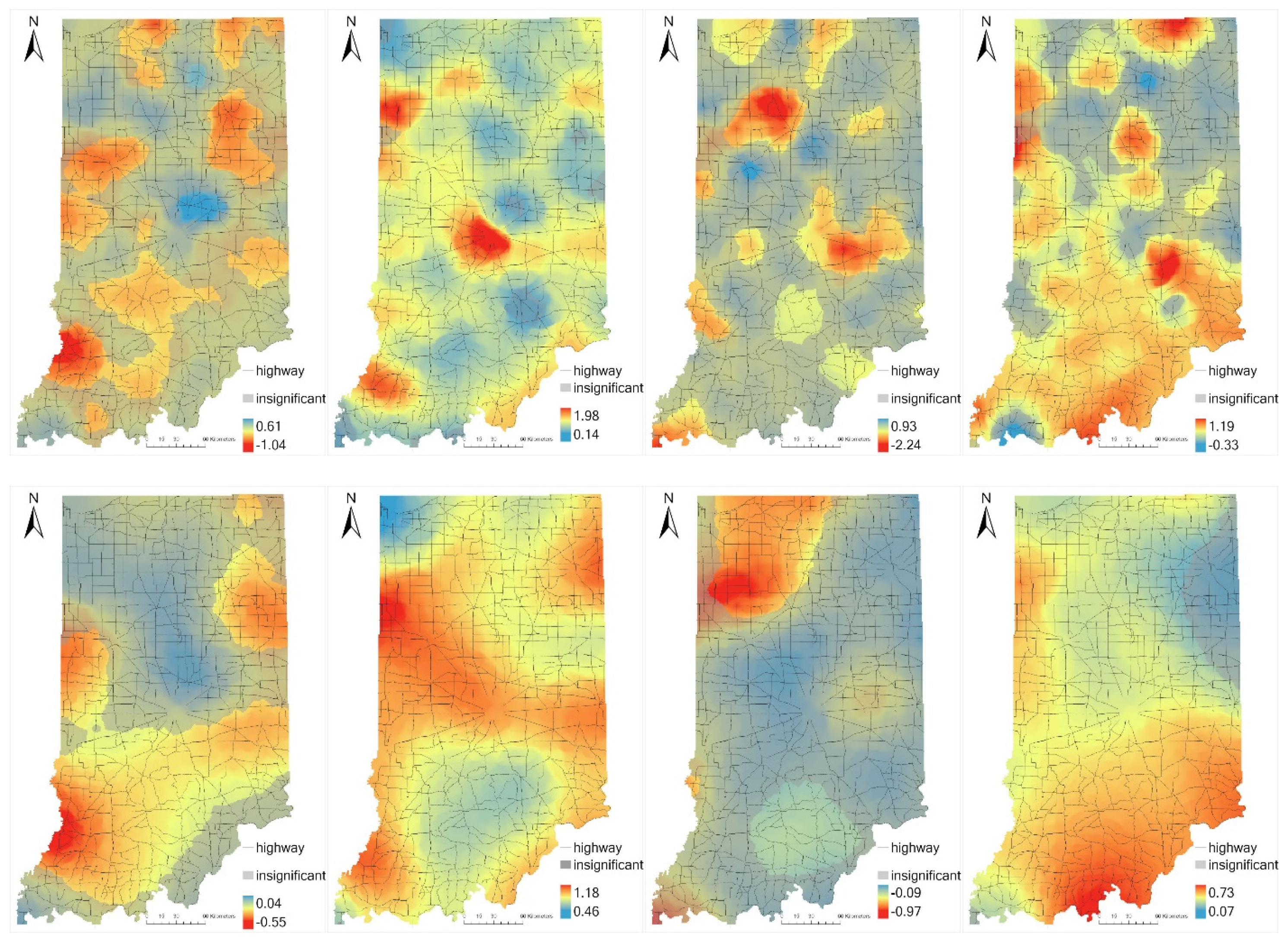
The distributions of local coefficient estimates and their significance interpolated by Inverse distance weighted (IDW) for GWPR, GWNBR, GWNBRg are plotted in Figure 2. Using the known parameter values for the 9415 curve segments, the IDW algorithm predicts values for unmeasured locations using the values of surrounding measured locations. The areas with a significance level of less than 90% are not considered in parameter analysis and covered up with gray color. Generally, each of the coefficient distributions of GWPR, GWNBR, or GWNBRg is more homogeneous as a result of their different optimum bandwidth. The larger their optimum bandwidth is, the more homogeneous their coefficient distributions will be.
Since GWNBR performs best with regard to the goodness of fit in terms of AICc, the parameter estimations are mainly illustrated according to the GWNBR model. Observations with significant coefficients account for 54.9%, 100%, 22.0%, and 96.2% for LOGR, LOGL, LOGF, and LOGA, respectively. A high percentage of parameter significance of LOGL and LOGA appear as expected due to the predominant influence of exposure factors in crash frequency prediction.
Observing from the curve radius (LOGR) coefficient distribution from GWPR in Figure 2a, the central area presents the highest coefficients, but only a small area shows positive signs. However, central and northwestern regions with high coefficients do not present enough significance to be considered in the GWNBR model. In the GWNBR model, lower values mainly distribute in the southern part of Indiana state, indicating a significant influence of curve radius in these regions. For the GWPR model, Figure 2a shows several significant regions that are hard to summarize spatial patterns of the radius coefficient. GWNBRg in Figure 2a presents a smooth decrease from the northwest to the southwest, which may be caused by some extreme values. Hence, although 93% of observations show significant coefficients for the GWNBRg model of LOGR, the coefficient varying trend may not be reliable.
For the curve segment length (LOGL) in Figure 2b, the GWNBR coefficient distribution presents two relatively lower coefficients regions in southern Indiana and the area close to Chicago. Similar to the LOGR coefficient distribution, Figure 2b GWPR presents a broken distribution of LOGL coefficient with no apparent pattern, and Figure 2b GWNBRg shows a decrease of the coefficient from center to north and south.
When analyzing the spatial distribution of GWNBR coefficients for curve friction (LOGF) in Figure 2c, it is observed that there are only two separate regions showing significant coefficients. The one located in the southern area that almost coincides with LOGL southern low coefficient area in Figure 2b GWNBR has coefficient values around −0.25, while the other one located in the north area has significantly lower friction coefficients.
In Figure 2d, the AADT (LOGA) coefficient distribution of GWNBR demonstrates high values in the south and southeast of Indiana. There also exists a small area of the non-significant coefficient area in the northeast. About the GWPR model in Figure 2d, an insignificant coefficient area is mainly located in the north of Indiana. GWNBRg (bottom row) presents a more general coefficient decreasing trend from south to north.
In summary, coefficient distributions in GWPR and GWNBRg have their disadvantages associated with parameter explanation. All coefficients display a very heterogeneous pattern in the GWPR modeling, while the distribution of the coefficient of GWNBRg is very homogeneous. Even without considering its worst goodness of fit, the GWPR coefficient distributions are excessively detailed for analysis. On the contrary, the GWNBRg coefficient distributions show a state-wide smooth surface with small variation, and almost all observations have significant coefficients for these four parameters. However, this characteristic drives GWNBRg closer to a global model that could not elaborate spatial heterogeneity of the parameters. The optimum bandwidth of GWNBR is moderate and thereby shows a more explainable parameter distribution map than the other two GWR models.
5.4. Local Analysis of GWR Results
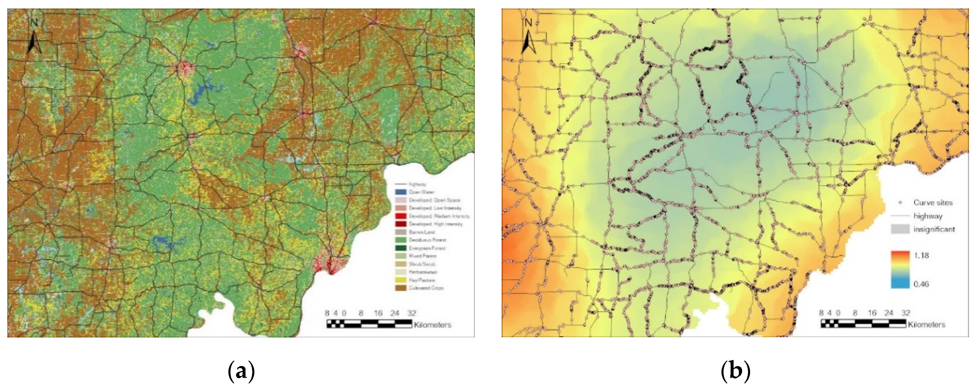
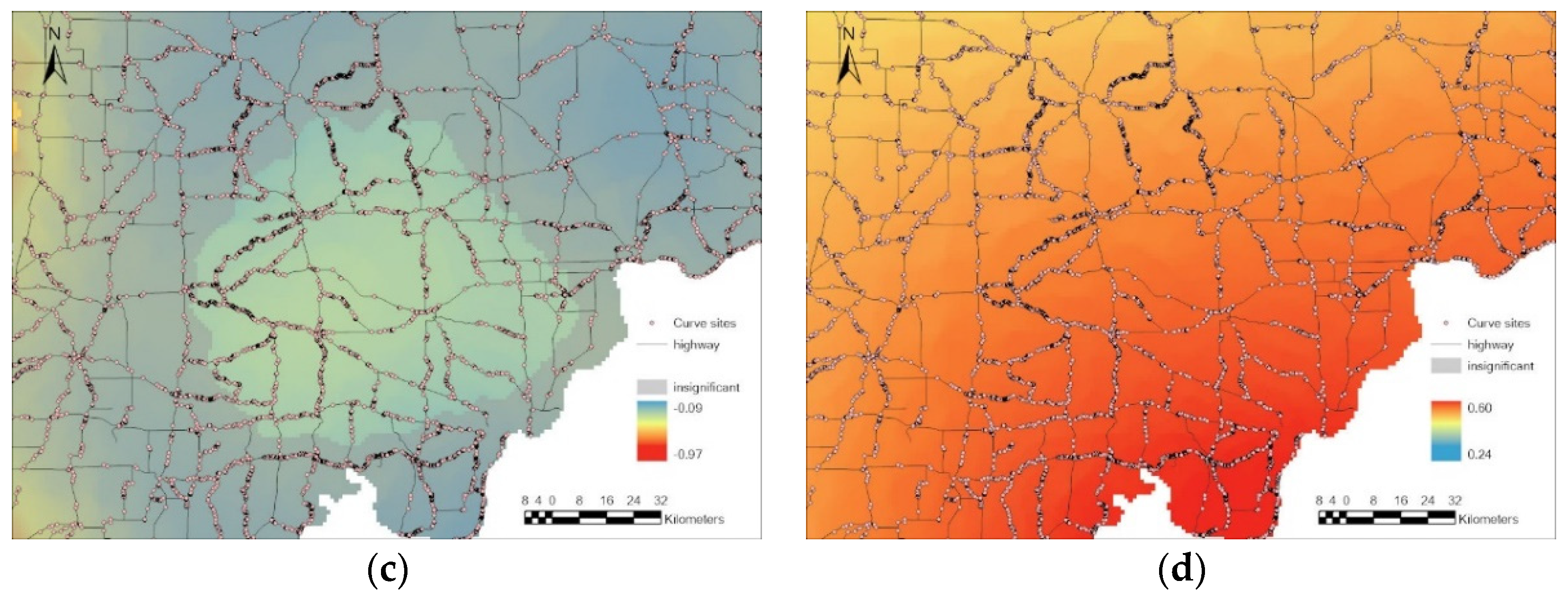
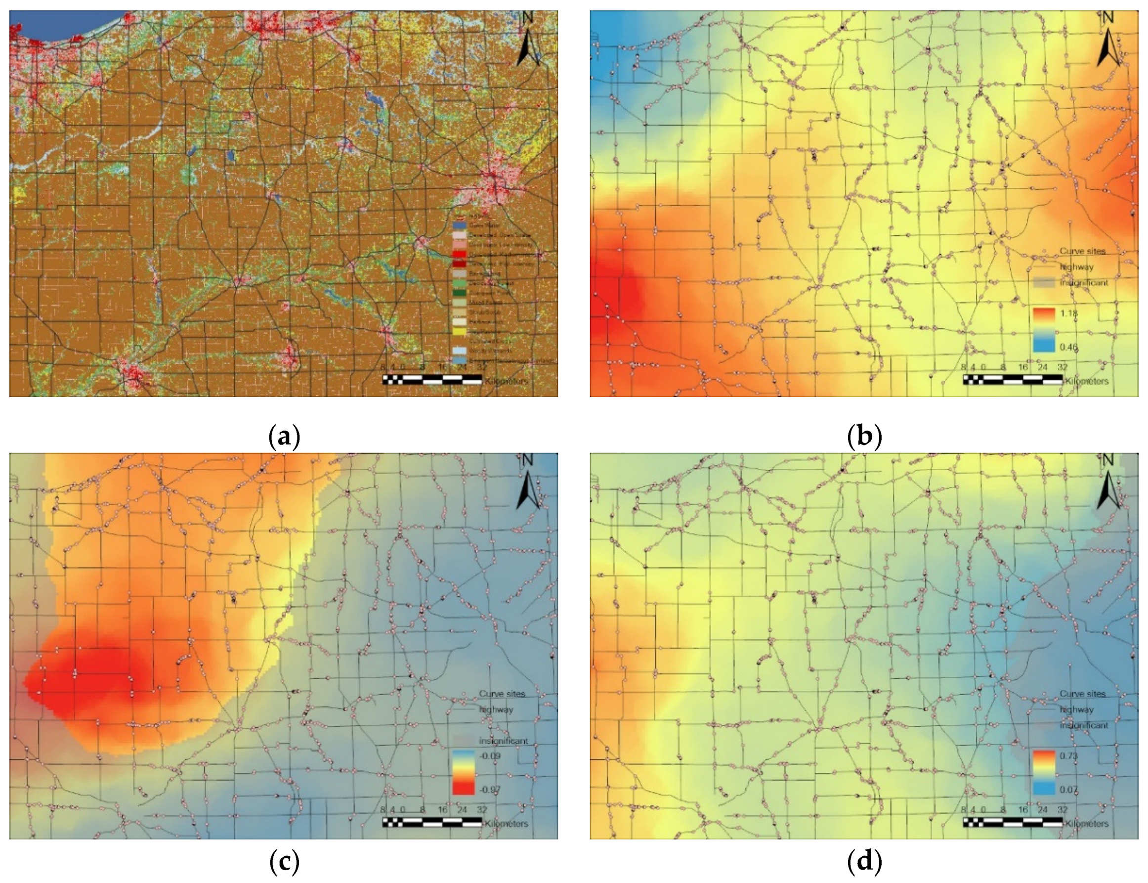
Observing the differences between coefficient distributions in north and south Indiana, it is necessary to take local examples to analyze possible factors that caused the heterogeneity. As described in the introduction, there are plenty of unobserved factors, including driver’s response, climate, and landcover. This paper found that the landcover pattern coincides with the coefficient distribution of pavement friction and curve length, which can be illustrated by two typical regions of Indiana with different land covers and topographies.
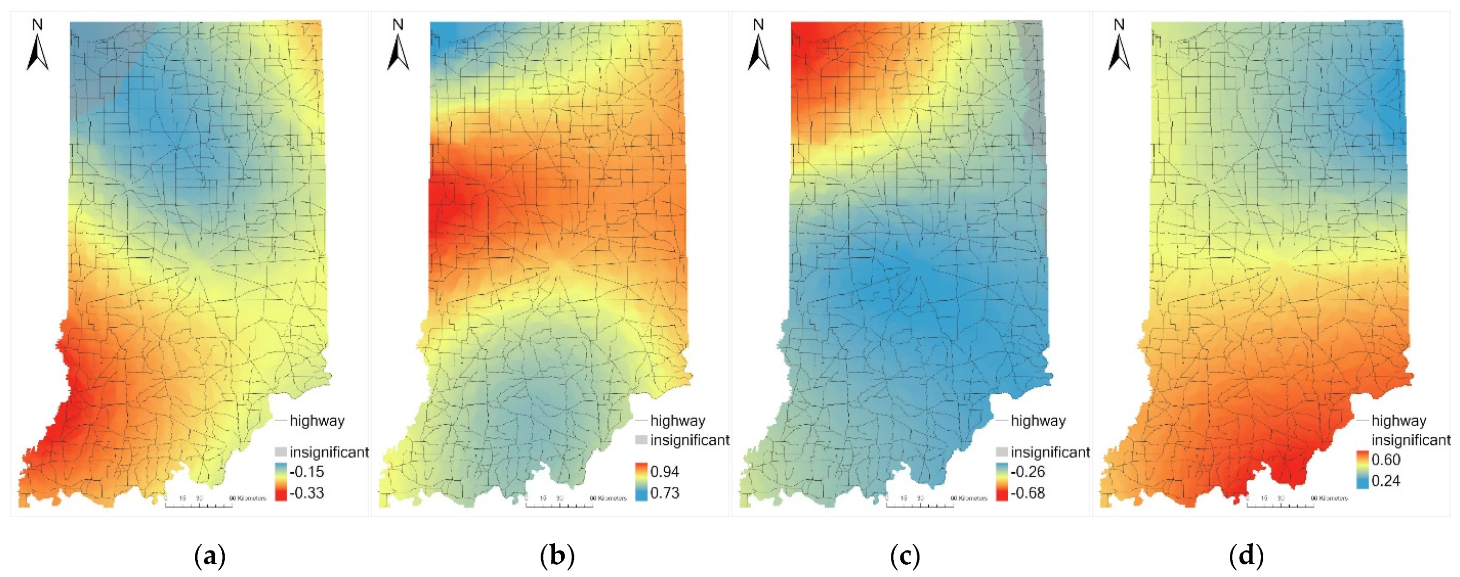
Taking southern Indiana with an area of forest and northern Indiana with cultivated crops for comparison, there are some coefficient distribution patterns matching the landcover in Figure 3a and Figure 4a. In the southern Indiana forest region, this area has a higher absolute value for AADT coefficients and low absolute values for curve length and pavement friction coefficient, which reflects the relatively strong influence of traffic volume on the curve crash frequency in forest curve segments. In northern Indiana, with homogenous land cover, the parameters vary over space. Comparing with the southern Indiana forest area, the coefficients of AADT and the coefficients of pavement friction in areas with significant coefficients are significantly lower at a 95% confidence level. The absolute value of pavement friction coefficient in the forest area is around 75% less than that of the northern plain area. However, landcover could not serve as a variable in models as all of these curve segments are located in developed open space without varying landcover distributed around them.
In respect of curve distribution density, there are also patterns observed from Figure 4. For the area with significant coefficients in Figure 4c, the locations with sparse curve segment distribution show higher absolute values of pavement friction coefficient than the rest area at a 95% confidence level. Considering it is also a low population density cultivated cropland, it is explainable that pavement friction highly influences the curve crash frequency in sparsely populated fields, where highways are mostly straight.
Based on the three-years of curve crash records on Indiana highways, we can draw a conclusion that crash frequency depends less on friction and curve length but has much to do with AADT in the southern forest area. The rest of Indiana state with mostly cultivated crop landcover still has some other unobserved factors, like curve density, that may affect the curve crash frequency. This paper indicates that higher friction surface treatment (HFST) is highly recommended for highway curve segments in Indiana plain areas for safety improvement.
Generally, planners can directly use the results obtained from the spatial distribution analysis of GWNBR coefficients to develop security enhancement strategies in curve design and evaluate and prioritize these strategies from the perspective of security effects.
6. Conclusions
Over-dispersed crash frequency with spatial heterogeneity was employed to quantitively investigate its relationship with curve segment characteristics aggregated at microlevel (each observation). Two types of methods, non-spatial models and spatial models, were utilized to account for the spatial heterogeneity of coefficients due to unobserved factors over space. To consider data overdispersion, the traditional NB model is specified as a basic global model. RPNB and GWR spatial approaches, including GWPR, GWNBR, and GWNBRg were used to find out the preferable model for explaining road crash occurrence. The estimated model to determine the crash frequency occurring on the curves uses explanatory variables of curve radius, curve length, pavement friction, and traffic volume, aggregated in individual curve segments.
The GWPR yields the lowest MAD (0.845) and the smallest absolute value of Moran’s I (0.0297) by overfitting to extreme values with its coefficient heterogeneity, while the GWNBR model outperforms others in terms of log-likelihood (−9780.7) and AICc (19,715.6). Since none of these models proves non-autocorrelation of residual spatial distribution, GWNBR was the best approach that was able to capture the spatial heterogeneity between the frequency of curve crashes and the explanatory variables. Although the RPNB model can incorporate unobserved heterogeneity in the modeling process and has been widely employed, it fails to account for the spatial correlation that existed across adjacent observations, which may result in biased parameter estimates and incorrect inference. The calibration process of the GWR approach is based on the First Law of Geography, which is implemented as all attribute values over the area of interest are correlated, but near values are more related than distant values. The GWPR model can minimize MAD by heterogeneous coefficient distribution pattern, but with significant incorrect signs for radius and friction, there might exist overfitting issues. The GWNBR model has better performance than the GWNBRg model with a global dispersion parameter; it is selected as the best local model depicting non-stationary curve crash frequency coefficients state-wide.
The GWNBR model presents a moderate fluctuation of curve segments radius and pavement friction influence for crash frequency over space, suggesting spatial heterogeneity on both parameters. For the southern Indiana forest area, pavement friction and curve length play a less critical role in reducing crash occurrence than other landcover regions, but AADT is more crucial in this area. In plain areas, parameters still vary over space without considering other unobserved factors such as weather and driver behavior. It was found that pavement friction effect on crash reduction in south forest area is 75% less than north plain area. These findings will help safety professionals to more accurately estimate the safety of horizontal curves, allocate funds to reduce or prevent potential crashes, and design better road segments based on existing horizontal curve crash data to minimize crash risk. For example, HFST is suggested to be implemented to highway curves in the plain region. In the hilly areas, some countermeasures such as limiting traffic volume in peak hours should be considered at the same time while implementing HFST if the terrain does not allow the curve radius to decrease.
This paper has some limitations. Since Indiana is dominated by cultivated crops and forests, it is difficult to reliably infer the effects of parameters in other less represented land covers. Furthermore, speed limit data are an important factor for a curve safety study. Although a non-stationary model could compensate for unavailable variables, adding speed limit data would possibly lead to more realistic modeling.
There are several areas recommended for future work. It is not always true that all parameters are spatial-varying when too many variables are involved. Hence, a semi-parametric model can be considered for setting variables without strong spatial variation. To account for local effects in both space and time, the extension of the GWR approach to the temporal domain, that is, the GTWR model [33,60], might be a reasonable model for traffic safety studies. Finally, as there are excessive zero count observations, a zero-inflated model might be combined with the conventional GWR model, that is, a zero-inflated geographically weighted negative binomial regression (ZIGWNBR) model can be considered.
Author Contributions
Conceptualization, Jie Shan, Ce Wang, and Shuo Li; methodology, Jie Shan, Ce Wang; software, Ce Wang; validation, Ce Wang, Jie Shan, and Shuo Li; formal analysis, Ce Wang, Shuo Li, Jie Shan, investigation, Ce Wang; resources, Shuo Li; data curation, Ce Wang; writing—original draft preparation, Ce Wang; writing—review and editing, Ce Wang, Jie Shan, Shuo Li; visualization, Ce Wang; supervision, Jie Shan and Shuo Li; project administration, Jie Shan and Shuo Li; funding acquisition, Jie Shan and Shuo Li. All authors have read and agreed to the published version of the manuscript.
Funding
Please add: This work was sponsored by the Indiana Department of Transportation in cooperation with the Federal Highway Administration (FHWA) through the Joint Transportation Research Program (JTRP) of Indiana DOT and Purdue University.
Data Availability Statement
Some of the data used in this paper are publicly available. Indiana AADT data can be found here (accessd at 20 May 2020): [https://www.in.gov/indot/2469.htm]. Indiana street centerlines shapefile data can be found here (accessed at 28 March 2021): [https://maps.indiana.edu/layerGallery.html?category=Streets]. Indiana highway pavement friction data were requested from INDOT. Restrictions apply to the availability of crash data, which was obtained from the Automated Reporting Information Exchange System and are available (accessed at 15 July 2019) [https://www.ariesportal.com/] with the permission of the Automated Reporting Information Exchange System (ARIES).
Conflicts of Interest
The authors declare no conflict of interest.
References
- Low-Cost Treatments for Horizontal Curve Safety 2016–Safety|Federal Highway Administration. Available online: https://safety.fhwa.dot.gov/roadway_dept/countermeasures/horicurves/fhwasa15084/#toc (accessed on 11 March 2021).
- Buddhavarapu, P.; Banerjee, A.; Prozzi, J.A. Influence of Pavement Condition on Horizontal Curve Safety. Accid. Anal. Prev. 2013, 52, 9–18. [Google Scholar] [CrossRef]
- Schneider, W.H.; Savolainen, P.T.; Moore, D.N. Effects of Horizontal Curvature on Single-Vehicle Motorcycle Crashes along Rural Two-Lane Highways. Transp. Res. Rec. 2010, 2194, 91–98. [Google Scholar] [CrossRef]
- Musey, K.; Park, S. Pavement Skid Number and Horizontal Curve Safety. Procedia Eng. 2016, 145, 828–835. [Google Scholar] [CrossRef] [Green Version]
- Gooch, J.P.; Gayah, V.V.; Donnell, E.T. Quantifying the Safety Effects of Horizontal Curves on Two-Way, Two-Lane Rural Roads. Accid. Anal. Prev. 2016, 92, 71–81. [Google Scholar] [CrossRef] [PubMed]
- Venkataraman, N.; Shankar, V.; Ulfarsson, G.F.; Deptuch, D. A Heterogeneity-in-Means Count Model for Evaluating the Effects of Interchange Type on Heterogeneous Influences of Interstate Geometrics on Crash Frequencies. Anal. Methods Accid. Res. 2014, 2, 12–20. [Google Scholar] [CrossRef]
- Mannering, F.L.; Shankar, V.; Bhat, C.R. Unobserved Heterogeneity and the Statistical Analysis of Highway Accident Data. Anal. Methods Accid. Res. 2016, 11, 1–16. [Google Scholar] [CrossRef]
- Cai, Q.; Abdel-Aty, M.; Lee, J.; Huang, H. Integrating Macro- and Micro-Level Safety Analyses: A Bayesian Approach Incorporating Spatial Interaction. Transp. Transp. Sci. 2019, 15, 285–306. [Google Scholar] [CrossRef]
- Wan, D. The Spatial Analysis of Crash Frequency and Injury Severities in New York City: Applications of Geographically Weighted Regression Method. Ph.D. Thesis, The City College of New York, New York, NY, USA, 2018. [Google Scholar]
- Duddu, V.R.; Pulugurtha, S.S. Neural Networks to Estimate Crashes at Zonal Level for Transportation Planning. In Proceedings of the European Transport Conference 2012, Glasgow, Scotland, 8–10 October 2012. [Google Scholar]
- Lee, J.; Abdel-Aty, M.; Jiang, X. Development of Zone System for Macro-Level Traffic Safety Analysis. J. Transp. Geogr. 2014, 38, 13–21. [Google Scholar] [CrossRef]
- Gomes, M.J.T.L.; Cunto, F.; da Silva, A.R. Geographically Weighted Negative Binomial Regression Applied to Zonal Level Safety Performance Models. Accid. Anal. Prev. 2017, 106, 254–261. [Google Scholar] [CrossRef] [PubMed]
- Soroori, E.; Moghaddam, A.M.; Salehi, M. Modeling Spatial Nonstationary and Overdispersed Crash Data: Development and Comparative Analysis of Global and Geographically Weighted Regression Models Applied to Macrolevel Injury Crash Data. J. Transp. Saf. Secur. 2020, 1–25. [Google Scholar] [CrossRef]
- Aguero-Valverde, J.; Jovanis, P.P. Spatial Analysis of Fatal and Injury Crashes in Pennsylvania. Accid. Anal. Prev. 2006, 38, 618–625. [Google Scholar] [CrossRef] [PubMed]
- Huang, H.; Abdel-Aty, M.A.; Darwiche, A.L. County-Level Crash Risk Analysis in Florida: Bayesian Spatial Modeling. Transp. Res. Rec. 2010, 2148, 27–37. [Google Scholar] [CrossRef]
- Abdel-Aty, M.; Lee, J.; Siddiqui, C.; Choi, K. Geographical Unit Based Analysis in the Context of Transportation Safety Planning. Transp. Res. Part A Policy Pract. 2013, 49, 62–75. [Google Scholar] [CrossRef]
- Quddus, M.A. Modelling Area-Wide Count Outcomes with Spatial Correlation and Heterogeneity: An Analysis of London Crash Data. Accid. Anal. Prev. 2008, 40, 1486–1497. [Google Scholar] [CrossRef] [PubMed] [Green Version]
- Wang, C.; Quddus, M.; Ison, S. The Effects of Area-Wide Road Speed and Curvature on Traffic Casualties in England. J. Transp. Geogr. 2009, 17, 385–395. [Google Scholar] [CrossRef] [Green Version]
- Rahman, M.T.; Jamal, A.; Al-Ahmadi, H.M. Examining Hotspots of Traffic Collisions and Their Spatial Relationships with Land Use: A GIS-Based Geographically Weighted Regression Approach for Dammam, Saudi Arabia. ISPRS Int. J. Geo-Inf. 2020, 9, 540. [Google Scholar] [CrossRef]
- Amoh-Gyimah, R.; Saberi, M.; Sarvi, M. Macroscopic Modeling of Pedestrian and Bicycle Crashes: A Cross-Comparison of Estimation Methods. Accid. Anal. Prev. 2016, 93, 147–159. [Google Scholar] [CrossRef] [PubMed]
- Amoh-Gyimah, R.; Sarvi, M.; Saberi, M. Investigating the Effects of Traffic, Socioeconomic, and Land Use Characteristics on Pedestrian and Bicycle Crashes: A Case Study of Melbourne, Australia. In Proceedings of the Transportation Research Board 95th Annual Meeting, Washington, DC, USA, 10–14 January 2016. [Google Scholar]
- Amoh-Gyimah, R.; Saberi, M.; Sarvi, M. The Effect of Variations in Spatial Units on Unobserved Heterogeneity in Macroscopic Crash Models. Anal. Methods Accid. Res. 2017, 13, 28–51. [Google Scholar] [CrossRef]
- Anastasopoulos, P.C.; Mannering, F.L. An Empirical Assessment of Fixed and Random Parameter Logit Models Using Crash- and Non-Crash-Specific Injury Data. Accid. Anal. Prev. 2011, 43, 1140–1147. [Google Scholar] [CrossRef] [PubMed]
- Ziakopoulos, A.; Yannis, G. A Review of Spatial Approaches in Road Safety. Accid. Anal. Prev. 2020, 135, 105323. [Google Scholar] [CrossRef] [PubMed]
- Hadayeghi, A.; Shalaby, A.S.; Persaud, B.N. Development of Planning Level Transportation Safety Tools Using Geographically Weighted Poisson Regression. Accid. Anal. Prev. 2010, 42, 676–688. [Google Scholar] [CrossRef] [PubMed]
- Sun, Y. Functional-Coefficient Spatial Autoregressive Models with Nonparametric Spatial Weights. J. Econom. 2016, 195, 134–153. [Google Scholar] [CrossRef]
- El-Basyouny, K.; Sayed, T. Urban Arterial Accident Prediction Models with Spatial Effects. Transp. Res. Rec. 2009, 2102, 27–33. [Google Scholar] [CrossRef]
- Xu, P.; Huang, H. Modeling Crash Spatial Heterogeneity: Random Parameter versus Geographically Weighting. Accid. Anal. Prev. 2015, 75, 16–25. [Google Scholar] [CrossRef] [PubMed]
- Marek, L.; Campbell, M.; Epton, M.; Kingham, S.; Storer, M. Winter Is Coming: A Socio-Environmental Monitoring and Spatiotemporal Modelling Approach for Better Understanding a Respiratory Disease. ISPRS Int. J. Geo-Inf. 2018, 7, 432. [Google Scholar] [CrossRef] [Green Version]
- Chen, J.; Liu, L.; Xiao, L.; Xu, C.; Long, D. Integrative Analysis of Spatial Heterogeneity and Overdispersion of Crime with a Geographically Weighted Negative Binomial Model. ISPRS Int. J. Geo-Inf. 2020, 9, 60. [Google Scholar] [CrossRef] [Green Version]
- Wang, D.; Yang, Y.; Qiu, A.; Kang, X.; Han, J.; Chai, Z. A CUDA-Based Parallel Geographically Weighted Regression for Large-Scale Geographic Data. ISPRS Int. J. Geo-Inf. 2020, 9, 653. [Google Scholar] [CrossRef]
- Li, Z.; Fotheringham, A.S.; Li, W.; Oshan, T. Fast Geographically Weighted Regression (FastGWR): A Scalable Algorithm to Investigate Spatial Process Heterogeneity in Millions of Observations. Int. J. Geogr. Inf. Sci. 2019, 33, 155–175. [Google Scholar] [CrossRef]
- Fotheringham, A.S.; Crespo, R.; Yao, J. Geographical and Temporal Weighted Regression (GTWR). Geogr. Anal. 2015, 47, 431–452. [Google Scholar] [CrossRef] [Green Version]
- Hadayeghi, A.; Shalaby, A.S.; Persaud, B. Macrolevel Accident Prediction Models for Evaluating Safety of Urban Transportation Systems. Transp. Res. Rec. 2003, 1840, 87–95. [Google Scholar] [CrossRef]
- Li, Z.; Wang, W.; Liu, P.; Bigham, J.M.; Ragland, D.R. Using Geographically Weighted Poisson Regression for County-Level Crash Modeling in California. Saf. Sci. 2013, 58, 89–97. [Google Scholar] [CrossRef]
- Nakaya, T.; Fotheringham, A.S.; Brunsdon, C.; Charlton, M. Geographically Weighted Poisson Regression for Disease Association Mapping. Stat. Med. 2005, 24, 2695–2717. [Google Scholar] [CrossRef] [PubMed] [Green Version]
- da Silva, A.R.; Rodrigues, T.C.V. Geographically Weighted Negative Binomial Regression—Incorporating Overdispersion. Stat. Comput. 2013. [Google Scholar] [CrossRef]
- Shaon, M.R.R.; Qin, X.; Shirazi, M.; Lord, D.; Geedipally, S.R. Developing a Random Parameters Negative Binomial-Lindley Model to Analyze Highly over-Dispersed Crash Count Data. Anal. Methods Accid. Res. 2018, 18, 33–44. [Google Scholar] [CrossRef]
- Shaon, M.R.R.; Schneider, R.J.; Qin, X.; He, Z.; Sanatizadeh, A.; Flanagan, M.D. Exploration of Pedestrian Assertiveness and Its Association with Driver Yielding Behavior at Uncontrolled Crosswalks. Transp. Res. Rec. 2018, 2672, 69–78. [Google Scholar] [CrossRef]
- Chen, S.; Saeed, T.U.; Alqadhi, S.D.; Labi, S. Safety Impacts of Pavement Surface Roughness at Two-Lane and Multi-Lane Highways: Accounting for Heterogeneity and Seemingly Unrelated Correlation across Crash Severities. Transp. Transp. Sci. 2019, 15, 18–33. [Google Scholar] [CrossRef]
- Venkataraman, N.S.; Ulfarsson, G.F.; Shankar, V.; Oh, J.; Park, M. Model of Relationship between Interstate Crash Occurrence and Geometrics: Exploratory Insights from Random Parameter Negative Binomial Approach. Transp. Res. Rec. 2011, 2236, 41–48. [Google Scholar] [CrossRef]
- Venkataraman, N.; Ulfarsson, G.F.; Shankar, V.N. Random Parameter Models of Interstate Crash Frequencies by Severity, Number of Vehicles Involved, Collision and Location Type. Accid. Anal. Prev. 2013, 59, 309–318. [Google Scholar] [CrossRef] [PubMed]
- Chen, E.; Tarko, A.P. Modeling Safety of Highway Work Zones with Random Parameters and Random Effects Models. Anal. Methods Accid. Res. 2014, 1, 86–95. [Google Scholar] [CrossRef]
- Saeed, T.U.; Hall, T.; Baroud, H.; Volovski, M.J. Analyzing Road Crash Frequencies with Uncorrelated and Correlated Random-Parameters Count Models: An Empirical Assessment of Multilane Highways. Anal. Methods Accid. Res. 2019, 23, 100101. [Google Scholar] [CrossRef]
- Xin, C.; Wang, Z.; Lee, C.; Lin, P.-S. Modeling Safety Effects of Horizontal Curve Design on Injury Severity of Single-Motorcycle Crashes with Mixed-Effects Logistic Model. Transp. Res. Rec. 2017, 2637, 38–46. [Google Scholar] [CrossRef]
- Xin, C.; Wang, Z.; Lin, P.-S.; Lee, C.; Guo, R. Safety Effects of Horizontal Curve Design on Motorcycle Crash Frequency on Rural, Two-Lane, Undivided Highways in Florida. Transp. Res. Rec. 2017, 2637, 1–8. [Google Scholar] [CrossRef]
- Mannering, F.L.; Bhat, C.R. Analytic Methods in Accident Research: Methodological Frontier and Future Directions. Anal. Methods Accid. Res. 2014, 1, 1–22. [Google Scholar] [CrossRef]
- Agresti, A. Foundations of Linear and Generalized Linear Models; John Wiley & Sons: Hoboken, NJ, USA, 2015; ISBN 978-1-118-73005-8. [Google Scholar]
- Hilbe, J.M. Negative Binomial Regression; Cambridge University Press: Cambridge, UK, 2011; ISBN 978-0-521-19815-8. [Google Scholar]
- Fotheringham, A.S.; Brunsdon, C.; Charlton, M. Geographically Weighted Regression: The Analysis of Spatially Varying Relationships; John Wiley & Sons: Hoboken, NJ, USA, 2003; ISBN 978-0-470-85525-6. [Google Scholar]
- Imprialou, M.; Quddus, M. Crash Data Quality for Road Safety Research: Current State and Future Directions. Accid. Anal. Prev. 2019, 130, 84–90. [Google Scholar] [CrossRef] [PubMed] [Green Version]
- Romero, M.; Atisso, E.; Wang, T.; Slusher, L.; Tarko, A. Using GIS to Determine Locations for Safety Improvements. Available online: https://docs.lib.purdue.edu/purduegisday/2017/allevents/1/ (accessed on 26 April 2021).
- Bíl, M.; Andrášik, R.; Sedoník, J.; Cícha, V. ROCA–An ArcGIS Toolbox for Road Alignment Identification and Horizontal Curve Radii Computation. PLoS ONE 2018, 13, e0208407. [Google Scholar] [CrossRef] [PubMed] [Green Version]
- Heiberger, R.M.; Holland, B. Statistical Analysis and Data Display; Springer Texts in Statistics; Springer: New York, NY, USA, 2015; ISBN 978-1-4939-2121-8. [Google Scholar]
- Elliott, A.C.; Hynan, L.S. A SAS® Macro Implementation of a Multiple Comparison Post Hoc Test for a Kruskal–Wallis Analysis. Comput. Methods Programs Biomed. 2011, 102, 75–80. [Google Scholar] [CrossRef] [PubMed]
- Moran, P.A.P. Notes on Continuous Stochastic Phenomena. Biometrika 1950, 37, 17–23. [Google Scholar] [CrossRef] [PubMed]
- Geedipally, S.R.; Pratt, M.P.; Lord, D. Effects of Geometry and Pavement Friction on Horizontal Curve Crash Frequency. J. Transp. Saf. Secur. 2019, 11, 167–188. [Google Scholar] [CrossRef]
- Himes, S.; Porter, R.J.; Hamilton, I.; Donnell, E. Safety Evaluation of Geometric Design Criteria: Horizontal Curve Radius and Side Friction Demand on Rural, Two-Lane Highways. Transp. Res. Rec. 2019, 2673, 516–525. [Google Scholar] [CrossRef]
- Fotheringham, A.S.; Oshan, T.M. Geographically Weighted Regression and Multicollinearity: Dispelling the Myth. J. Geogr. Syst. 2016, 18, 303–329. [Google Scholar] [CrossRef]
- Zhang, X.; Huang, B.; Zhu, S. Spatiotemporal Influence of Urban Environment on Taxi Ridership Using Geographically and Temporally Weighted Regression. ISPRS Int. J. Geo-Inf. 2019, 8, 23. [Google Scholar] [CrossRef] [Green Version]
Figure 1.
Curve segments distribution in Indiana (left) and typical examples on SR-114 (upper right) and SR-450 (lower right).
Figure 1.
Curve segments distribution in Indiana (left) and typical examples on SR-114 (upper right) and SR-450 (lower right).

Figure 2.
Distribution of (a) LOGR, (b) LOGL, (c) LOGF, and (d) LOGA in different GWPR (top), GWNBR (middle), and GWNBRg (bottom).
Figure 2.
Distribution of (a) LOGR, (b) LOGL, (c) LOGF, and (d) LOGA in different GWPR (top), GWNBR (middle), and GWNBRg (bottom).


Figure 3.
Landcover (a), distribution of (b) LOGL, (c) LOGF, and (d) LOGA in GWNBR in a forest area in southern Indiana.
Figure 3.
Landcover (a), distribution of (b) LOGL, (c) LOGF, and (d) LOGA in GWNBR in a forest area in southern Indiana.


Figure 4.
Landcover (a), distribution of (b) LOGL, (c) LOGF, and (d) LOGA in GWNBR in a plain area in northern Indiana.
Figure 4.
Landcover (a), distribution of (b) LOGL, (c) LOGF, and (d) LOGA in GWNBR in a plain area in northern Indiana.


Table 1.
Variable description and summary statistics.
| Variables | Description | Mean | Std. dev | Min | Max |
|---|---|---|---|---|---|
| Number of crashes occurred during 2016–2018 per curve segment | 0.740 | 1.755 | 0 | 34 | |
| Radii of curve segments in meter | 354.10 | 199.61 | 25.21 | 999.64 | |
| Friction of pavement on curve segments at 40 mph | 43.80 | 15.12 | 8.20 | 104.20 | |
| Length of curve segments in meter | 104.05 | 109.92 | 30.49 | 1249.77 | |
| Mean of Annual Average Daily Traffic in 2016–2018 | 4214.16 | 5393.82 | 32.21 | 82,244.85 |
Table 2.
Goodness of fit and residual spatial dependency for different models.
| Model | Bandwidth (km) | # of Parameter | MAD | Log Likelihood | AICc | Dispersion Parameter | Moran’s | -Value |
|---|---|---|---|---|---|---|---|---|
| NB | - | 5 | 0.881 | −9978.4 | 19,968.0 | 1.88 | 0.0769 | |
| RPNB | - | 11 | 0.847 | −9917.1 | 19,856.2 | 1.31 | 0.0753 | |
| GWPR | 15.45 | 295.1 | 0.845 | −10,805.9 | 22,219.9 | - | 0.0297 | |
| GWNBR | 34.65 | 76.5 | 0.859 | −9780.7 | 19,715.6 | - | 0.0569 | |
| GWNBRg | 76.01 | 22.7 | 0.869 | −9900.9 | 19,847.4 | 1.88 | 0.0634 |
Note: -value is the possibility of model residual random distribution over space.
Table 3.
Estimated parameters of NB, RPNB, GWPR models.
| Model | NB | RPNB | GWPR | ||||||||||
|---|---|---|---|---|---|---|---|---|---|---|---|---|---|
| Mean | Min | Lwr | Med | Upr | Max | Mean | Min | Lwr | Med | Upr | Max | ||
| Intercept | −5.96 | −6.25 | −6.33 | −6.26 | −6.25 | −6.23 | −5.82 | −6.14 | −22.17 | −8.21 | −6.00 | −4.32 | 3.56 |
| LOGR | −0.24 | −0.30 | −0.33 | −0.31 | −0.30 | −0.29 | −0.14 | −0.23 | −1.04 | −0.36 | −0.24 | −0.10 | 0.61 |
| LOGL | 0.87 | 0.96 | 0.94 | 0.95 | 0.96 | 0.96 | 1.07 | 0.87 | 0.137 | 0.68 | 0.85 | 1.05 | 1.98 |
| LOGF | −0.36 | −0.40 | −0.46 | −0.42 | −0.41 | −0.39 | 0.08 | −0.29 | −2.24 | −0.44 | −0.25 | −0.04 | 0.94 |
| LOGA | 0.49 | 0.48 | 0.46 | 0.48 | 0.48 | 0.49 | 0.61 | 0.47 | −0.34 | 0.35 | 0.51 | 0.61 | 1.24 |
Table 4.
Estimated parameters of GWNBR and GWNBRg models.
| Model | GWNBR | GWNBRg | ||||||||||
|---|---|---|---|---|---|---|---|---|---|---|---|---|
| Mean | Min | Lwr | Med | Upr | Max | Mean | Min | Lwr | Med | Upr | Max | |
| Intercept | −5.80 | −9.19 | −6.82 | −5.64 | −5.16 | −1.79 | −5.82 | −7.07 | −6.42 | −6.01 | −5.66 | −3.45 |
| LOGR | −0.24 | −0.55 | −0.30 | −0.25 | −0.18 | 0.04 | −0.24 | −0.33 | −0.27 | −0.24 | −0.23 | −0.15 |
| LOGL | 0.85 | 0.46 | 0.76 | 0.85 | 0.93 | 1.18 | 0.84 | 0.73 | 0.80 | 0.83 | 0.87 | 0.94 |
| LOGF | −0.31 | −0.97 | −0.33 | −0.28 | −0.24 | −0.03 | −0.33 | −0.68 | −0.34 | −0.30 | −0.27 | −0.26 |
| LOGA | 0.46 | 0.07 | 0.36 | 0.47 | 0.57 | 0.73 | 0.48 | 0.24 | 0.40 | 0.51 | 0.55 | 0.60 |
Publisher’s Note: MDPI stays neutral with regard to jurisdictional claims in published maps and institutional affiliations. |
© 2021 by the authors. Licensee MDPI, Basel, Switzerland. This article is an open access article distributed under the terms and conditions of the Creative Commons Attribution (CC BY) license (https://creativecommons.org/licenses/by/4.0/).
Share and Cite
MDPI and ACS Style
Wang, C.; Li, S.; Shan, J. Non-Stationary Modeling of Microlevel Road-Curve Crash Frequency with Geographically Weighted Regression. ISPRS Int. J. Geo-Inf. 2021, 10, 286. https://doi.org/10.3390/ijgi10050286
AMA Style
Wang C, Li S, Shan J. Non-Stationary Modeling of Microlevel Road-Curve Crash Frequency with Geographically Weighted Regression. ISPRS International Journal of Geo-Information. 2021; 10(5):286. https://doi.org/10.3390/ijgi10050286
Chicago/Turabian StyleWang, Ce, Shuo Li, and Jie Shan. 2021. "Non-Stationary Modeling of Microlevel Road-Curve Crash Frequency with Geographically Weighted Regression" ISPRS International Journal of Geo-Information 10, no. 5: 286. https://doi.org/10.3390/ijgi10050286
Note that from the first issue of 2016, this journal uses article numbers instead of page numbers. See further details here.