Mobility Data Warehouses


1
Department of Information Engineering, Instituto Tecnológico de Buenos Aires, Lavardén 315, C1437FBG Ciudad Autónoma de Buenos Aires, Argentina
2
Department of Computer & Decision Engineering (CoDE), CP 165/15 Université Libre de Bruxelles, Avenue F. D. Roosevelt 50, B-1050 Brussels, Belgium
*
Author to whom correspondence should be addressed.
ISPRS Int. J. Geo-Inf. 2019, 8(4), 170; https://doi.org/10.3390/ijgi8040170
Submission received: 9 January 2019
/
Revised: 12 March 2019
/
Accepted: 29 March 2019
/
Published: 2 April 2019
(This article belongs to the Special Issue Distributed and Parallel Architectures for Spatial Data)
Abstract
:The interest in mobility data analysis has grown dramatically with the wide availability of devices that track the position of moving objects. Mobility analysis can be applied, for example, to analyze traffic flows. To support mobility analysis, trajectory data warehousing techniques can be used. Trajectory data warehouses typically include, as measures, segments of trajectories, linked to spatial and non-spatial contextual dimensions. This paper goes beyond this concept, by including, as measures, the trajectories of moving objects at any point in time. In this way, online analytical processing (OLAP) queries, typically including aggregation, can be combined with moving object queries, to express queries like “List the total number of trucks running at less than 2 km from each other more than 50% of its route in the province of Antwerp” in a concise and elegant way. Existing proposals for trajectory data warehouses do not support queries like this, since they are based on either the segmentation of the trajectories, or a pre-aggregation of measures. The solution presented here is implemented using MobilityDB, a moving object database that extends the PostgresSQL database with temporal data types, allowing seamless integration with relational spatial and non-spatial data. This integration leads to the concept of mobility data warehouses. This paper discusses modeling and querying mobility data warehouses, providing a comprehensive collection of queries implemented using PostgresSQL and PostGIS as database backend, extended with the libraries provided by MobilityDB.
1. Introduction
Moving objects [1] (MOs) are objects (e.g., cars, trucks, pedestrians) whose spatial features change continuously in time. The data produced by MOs (e.g., by using attached devices like GPSs and smartphones) can be analyzed in many ways, for example, to discover mobility patterns [2]. This is called mobility data analysis, a technique that is currently used in many related fields, like traffic management, transportation, car pooling applications, smart cities, etc.
The increasing availability of MO data has triggered the interest in mobility data analysis, which has been growing steadily year after year. Moving object data generally come in the form of long sequences of spatiotemporal coordinates . To facilitate analysis, these sequences are split into smaller portions of movement, called trajectories. Trajectories can be represented in two possible ways. A continuous trajectory represents the movement track of an object by means of a sequence of spatiotemporal points occurring within a certain interval, together with interpolation functions that allow computing the (approximate) position of the object at any instant. A discrete trajectory contains only a sequence of spatiotemporal points but no interpolation function can be defined.
Moving object databases are databases that store the positions of MOs at any point in time. Although these databases are appropriate for querying, for example, current movement, by means of queries like “which taxis are within ten minutes from Brussels Central Station”, they do not support, per se, complex analytical queries such as “For each month, list the total number of buses running at a speed higher than 60 km per hour for more than 40% of their total route.” For this, integration with, for example, data warehousing technologies, is needed, yielding the notion of mobility data warehouses. These are data warehouses that contain MO data that can be analyzed in conjunction with other kinds of data (e.g., spatial data), for instance, a road network, altitude data, and the kind.
To represent MOs, the definition of appropriate data types is needed. The notion of temporal type refers to a collection of data types that capture the evolution over time of base types and spatial types. For instance, temporal integers may be used to represent the evolution in the number of employees in a department. Analogously, a temporal point may represent the evolution in time of the position of a vehicle, reported by a GPS device, which would yield a temporal geometry of type point. Over these kind of data types, MO databases can be implemented. Thus, MobilityDB was developed (the demo of this database can be accessed at http://demo.mobilitydb.eu/, where also the manual with a full description of the data types is available). MobilityDB is a MO database (MOD), that builds on PostGIS (the spatial extension of PostgreSQL), that extends the type system of PostgreSQL and PostGIS with abstract data types (ADTs), in order to represent MO data. These ADTs are based on the notion of temporal types and their associated operations.
1.1. Mobility Data Warehouses
Conventional databases are used to support the day-to-day operations in an organization. The operations over these databases are usually denoted as online transactional processing (OLTP). To support data analysis, the notion of data warehousing was developed. A data warehouse (DW) collects large amounts of data from various data sources and reduces them to a form that can be used to analyze the behavior of an organization. DWs are based on the multidimensional model, which represents data as facts that can be analyzed along a collection of dimensions, composed of levels conforming aggregation hierarchies. The multidimensional model builds on the data cube abstraction, where the axes of the cubes are the dimensions, and the cells contain measure values. Typically, DWs are exploited by means of the online analitycal processing (OLAP) technique, which consists of a collection of operations that manipulate the data cube. The most popular OLAP operations are roll-up, which aggregates measure data along a dimension up to a certain aggregation level; drill-down, which is the inverse of the former; slice, which drops a dimension from the cube; and dice, which selects a sub-cube that satisfies a boolean condition.
Spatial data can represent geographic objects (e.g., mountains, cities), geographic phenomena (e.g., temperature, precipitation), etc. Similarly to conventional databases, spatial databases are typically used for operational applications in many different domains, rather than to support data analysis tasks. Spatial DWs (SDWs), on the other hand, combine spatial databases features and DW technologies, to provide more sophisticated data analysis, visualization, and manipulation capabilities. Thus, a SDW is a DW that is capable of representing, storing, and manipulating spatial data. Usually, to represent the extent of a spatial object, spatial data types are used. A SDW can thus take advantage of the operations associated with spatial data types, to allow queries like “give me the total number of theaters within one kilometer from my current position”.
Most DWs (either spatial or not) assume that only facts evolve in time. However, dimension data, like for instance, the category of a product, may also change across time. The most popular approach for tackling this issue is based on the notion of slowly changing dimensions [3]. An alternative approach for this issue is based on the concept of temporal databases. Built-in temporal semantics allow these kinds of databases to manage time-varying information. The combination of spatial and temporal databases and DWs leads to the notion of spatiotemporal DWs. Since MO are in essence spatiotemporal, adding MO data to a DW leads to the notion of mobility DWs. This is, in a nutshell, the problem addressed by this paper: modeling and querying mobility DWs by means of adding temporal types to spatial DWs.
1.2. Contributions and Motivation
The authors of this paper had previously defined the notion of spatiotemporal queries as queries that can be expressed by Klug’s relational algebra with aggregation, extended with spatial and moving types [4]. Based on this, the authors defined spatiotemporal DWs as DWs that support spatiotemporal queries. The classification in the referred work helps to characterize the different kinds of DW systems in terms of their expressiveness, and it is used in the discussion below.
Many efforts have been published under the concept of trajectory data warehouses [5,6,7]. These works basically propose storing, in the DW fact tables, aggregate measures (like the number of cars in a given latitude-longitude range), segments of trajectories, or spatiotemporal points, probably together with semantic information. It is therefore clear that these approaches do not qualify as trajectory or, equivalently, spatiotemporal DWs (according to the classification in [4]), since they do not support spatiotemporal queries, given that they do not include moving data types. For example, storing aggregate measures [6], does not allow queries like “total distance covered by all cars in Brussels”. Instead, they allow expressing queries like “average number of cars in downtown Brussels on Sunday mornings”. These approaches conform, in some sense, traditional spatial DWs. The other proposals (although implementations are not yet reported), aim at querying semantic trajectories, for example “total number of persons going from restaurants to theaters”. Even in the case where spatiotemporal points are stored, these represent the raw trajectories rather than moving types, and thus everything must be solved using relational operations. On the other hand, there are systems that implement MO databases, typically Secondo and Hermes. However, these systems are not aimed at building mobility DWs, therefore, implementing a mobility DW based on them is not a trivial task. Section 6 further elaborates on the discussion above.
The work presented in this paper extends and dramatically improves existing trajectory DW proposals. The implementation of MobilityDB gives the possibility of defining MOs as measures in a DW fact table. Integrating relational warehouse data with MO data allows realizing the notion of spatiotemporal queries defined in [4], as this paper will show through a collection of comprehensive examples. The resulting DW is called Mobility DW. In addition, the problem of conceptual and logical modeling of mobility DWs is also covered here. Throughout this paper, the well-known Northwind DW [8], extended with MO and spatial data, is used as a running example.
Note that although the work presented here is based on a centralized PostgresSQL database management system (DBMS), there are ongoing efforts to develop parallel version of this DBMS, from which MobilityDB (and therefore, the mobility DW studied in this paper) can benefit. Further, in a Big Data scenario, horizontal scalability is crucial. This has encouraged the development of a horizontally-scalable version of Postgres, called Postgres-XL, https://www.postgres-xl.org, which can handle mixed workloads, which include OLTP and OLAP queries, GIS queries, OLTP transactions, and so on. Last, but not least, the approach presented here can be extended to big data hadoop-based environments that are currently available, http://spatialhadoop.cs.umn.edu, http://esri.github.io/gis-tools-for-hadoop.
1.3. Paper Organization
In Section 2, the notion of temporal types is defined and explained. Section 3 describes the implementation of temporal types in MobilityDB. Section 4 studies the modeling of mobility DWs, also providing a background on DW design, for the non-expert readers, while Section 5 presents a comprehensive set of queries to illustrate how a mobility DW can be exploited. Section 6 discusses related work and compares such work against the present proposal, and Section 7 concludes the paper.
2. Background: Temporal Types
To make this paper self-contained, this section presents some basic concepts on temporal types. Many of the concepts and operations can be found in [1,8]. However, to develop MobilityDB, new operations had been defined, and are also explained here. Also, a syntax for these temporal types is introduced here.
Temporal types are functions that map time instants to values from a domain. They are implemented by means of applying a constructor temporal(·). For example, a value of type temporal(integer) is a continuous function f : instant → integer. Analogously, a temporal boolean is a function mapping instants to boolean values. In temporal databases terminology, several notions for time can be defined. The most popular ones are valid time and transaction time [9]. The former represents the time period during which a database fact is valid in the modeled reality. The latter is the time period during which a fact stored in the database is considered to be true. These are orthogonal concepts. In the remainder, valid time is considered.
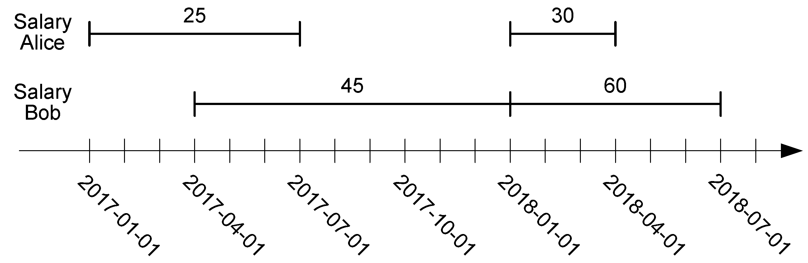
Temporal types may be undefined during certain time periods. For example, in Figure 1, Alice’s salary is undefined between 1 July 2017 and 1 January 2018 (e.g., because she took a six-month leave), and this is denoted ‘⊥’. As a convention, closed-open intervals are used.
2.1. Classes of Operations on Temporal Types
Temporal types are associated with different kinds of operations, described next.
Projection over domain and range. Operations of this kind are, for example, GetTime and GetValues, which return, respectively, the domain and range of a temporal type.
Interaction with domain and range. Example of operations of this kind are AtTimestamp, AtTimestampSet, AtPeriod, and AtPeriodSet, which restrict the function to a given timestamp (set) or period (set). Operations StartTimestamp and StartValue return, respectively, the first timestamp at which the function is defined and the corresponding value. The operations EndTimestamp and EndValue are analogous. The operations AtValue and AtRange restrict the temporal type to a value or to a range of values in the range of the function. The operations AtMin and AtMax restrict the function to the instants when its value is minimal or maximal, respectively.
Example 1.
The functions GetTime(SalaryAlice) and GetValues(SalaryAlice) return, respectively, {[2017-01-01, 2017-07-01), [2018-01-01, 2018-04-01)} and {25, 30}. Further, AtTimestamp(SalaryAlice, 2017-07-15) returns ‘⊥’, since Alice’s salary is undefined at that date. The operation StartTimestamp(SalaryAlice) returns 2017-01-01, while AtValue(SalaryAlice, 25) and AtValue(SalaryAlice, 35) return, respectively, a temporal real with value 20@[2017-01-01, 2017-07-01) and ‘⊥’, because no salary with value 35 exists.
Temporal aggregation. These kinds of operations are crucial to mobility data analysis. Three basic operations take as argument a temporal integer or real and return a real value namely: Integral, that returns the area under the curve defined by the function, Duration, which returns the duration of the temporal extent over which the function is defined, and Length, which returns the length of the curve defined by the function. From these operations, other derived operations can be defined, such as TWAvg, TWVariance, or TWStDev. The operation TWAvg computes the time-weighted average of a temporal value, taking into account the duration in which the function takes a value. TWVariance and TWStDev compute the variance and the standard deviation of a temporal type. Finally, MinValue and MaxValue return, respectively, the minimum and maximum value taken by the function. These can be obtained by Min(GetValues(·)) and Max(GetValues(·)) where Min and Max are the classic operations over numeric values.
Example 2.
In the example above, TAvg(SalaryAlice) would yield a value of 26.66, given that Alice had a salary of 25 during 181 days and a salary of 30 during 90 days.
Lifting. This class represents the generalization of the operations on nontemporal types to temporal types [10]. An operation for nontemporal types is lifted to allow any of the arguments to be replaced by a temporal type, and returns a temporal type. For example, the “less than” (<) operation has lifted versions (denoted by #<) where one or both of its arguments can be temporal types, yielding a temporal boolean. Intuitively, the result is computed at each instant using the nonlifted operation. When two temporal values are defined on different temporal extents, the result of a lifted operation can be defined either over the intersection of both extents or the union of them. In the remainder, for the lifted operations, the first option is assumed.
Example 3.
In Figure 1, the comparison SalaryAlice < SalaryBob results in a temporal boolean with value true@{[2017-04-01, 2017-07-01), [2018-01-01, 2018-04-01)}.
2.2. Temporal Types over Spatial Data
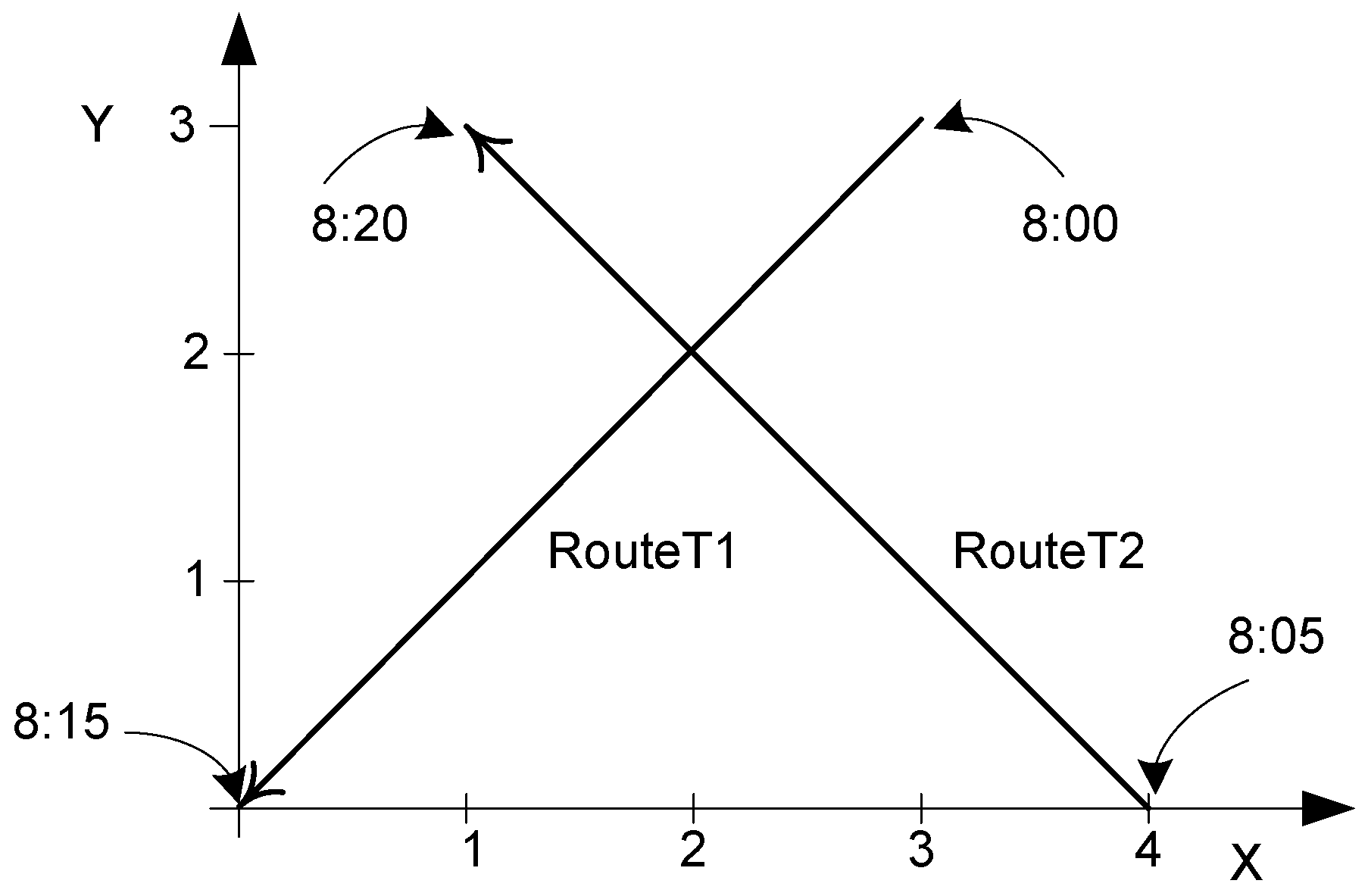
Temporal types can be also defined over spatial data types, not only over basic types like integers or reals. For example, the trajectory of a truck can be represented using a temporal(point) type. Analogously to what was explained above, this type would be a continuous function f : instant → point. Some of the operations described in Section 2.1 are explained next for the spatial case. The example in Figure 3 shows two temporal points RouteT1 and RouteT2 that represent the delivery routes of two trucks T1 and T2 on a particular day. It can be seen that, for instance, truck T1 took 15 min to go from point (3, 3) to point (0, 0), while truck T2 took 15 min to go from point (4, 0) to point (1, 3). A constant speed between consecutive pairs of points is assumed.
An operation called Trajectory, projects a temporal geometry into the plane. In the example, Trajectory(RouteT1) results in the leftmost line in Figure 3, without any temporal information. Note that the projection of a temporal point into the plane may consist in points and lines.
As an example of an operation of the class addressing the interaction with domain and range (as in Section 2.1) for the spatial case, the AtGeometry operation restricts the temporal point to a given geometry. For example, if Polygon denotes a polygon defined as follows Polygon((0 0, 0 2, 2 2, 2 0, 0 0)), then AtGeometry(RouteT1, Polygon) will return the value RouteT1 restricted to the period [8:05, 8:15].
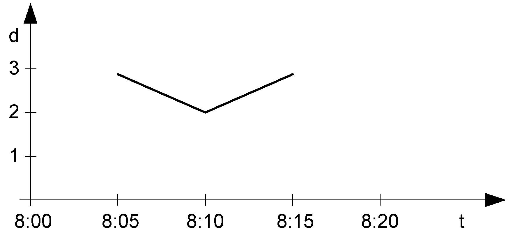
Analogously to the non-spatial case, all operations over nontemporal spatial types are lifted. For example, the Distance function has lifted versions where one or both of its arguments can be temporal points and the result is a temporal real. In the example, Distance(RouteT1, RouteT2) returns a temporal real shown in Figure 4, where, for instance, the value evolves from @8:05 to 2@8:10 to @8:15. Note that in this case, the distance function has been approximated by a linear function.
Lifted topological operations return a temporal boolean. Examples of such operators are TIntersects, TDWithin, and TContains. For example, TIntersects(RouteT1, RouteT2) returns a temporal boolean with value false@[8:05, 8:15] since the two trucks were never at the same point at any instant of their route. Similarly, TDWithin(RouteT1, RouteT2, 2) returns a temporal boolean with value {false@[8:05, 8:10), true@[8:10, 8:10], false@(8:10, 8:15]} since the two trucks were only at a distance of two at 8:10. Finally, if Polygon is defined as above, then TContains(Polygon, RouteT1) will return a temporal boolean with value {false@[8:00, 8:05), true@[8:05, 8:15]}.
To conclude, several operations compute the rate of change for points. Operation Speed yields the usual concept of speed of a temporal point at any instant as a temporal real. Operation Direction returns the direction of the movement, that is, the angle between the x-axis and the tangent to the trajectory of the moving point. Finally, the Turn operation yields the change of direction at any instant.
3. Temporal Types in MobilityDB
Temporal support has been introduced in the SQL standard, and implemented (in a limited way) in commercial database systems, by means of adding temporality to tables and associating a period with each row. Nevertheless, for mobility applications this approach does not suffice. For such applications, the temporal evolution of the attribute values is needed, along the lines of the data model proposed by Gadia and Nair [11]. This section describes the implementation in MobilityDB, of the temporal types presented in Section 2 as mentioned, a mobility database based on PostgreSQL and PostGIS. For full details, the reader is referred to the manual (http://demo.mobilitydb.eu/mobilitydb-manual.pdf).
3.1. Types in MobilityDB
In order to manipulate temporal types, MobilityDB uses the timestamptz (a shorthand for timestamp with time zone) type provided by PostgreSQL, and three new types: period, timestampset, and periodset. The period type is a specialized version of the tstzrange (short for timestamp with time zone range) type provided by PostgreSQL. Its functionality is similar to the one of type tstzrange, but with a more efficient implementation. A value of the period type has two bounds, the lower bound and the upper bound, which are timestamptz values. The bounds can be inclusive (represented by “[” and “]”), or exclusive (represented by “(” and “)”). A period value with equal and inclusive bounds corresponds to a timestamptz value. An example of a period value is as follows
SELECT period ‘[2017-01-01 08:00:00, 2017-01-03 09:30:00)’;The timestampset type represents a set of distinct timestamptz values. A timestampset value must contain at least one element, in which case it corresponds to a timestamptz value. The elements composing a timestampset value must be ordered. An example of a timestampset value is as follows
SELECT timestampset ‘{2017-01-01 08:00:00, 2017-01-03 09:30:00}’;Finally, the periodset type represents a set of disjoint period values. A periodset value must contain at least one element, in which case it corresponds to a period value. The elements composing a periodset value must be ordered. An example of a periodset value is as follows
SELECT periodset ‘{[2017-01-01 08:00:00, 2017-01-01 08:10:00],
            [2017-01-01 08:20:00, ’2017-01-01 08:40:00]}’;
Currently, MobilityDB provides six built-in temporal types, tbool, tint, tfloat, ttext, tgeompoint, and tgeogpoint, which are, respectively, based on the bool, int, float, and text types provided by PostgreSQL, as well as the geometry and geography types provided by PostGIS (the last two types restricted to 2D and 3D points). Temporal types may be discrete or continuous. Discrete temporal types (which are based on the boolean, int, or text types) evolve in a stepwise manner, while continuous temporal types (which are based on the float, geometry, or geography types) evolve in a continuous manner. The duration of a temporal value indicates the temporal extent at which the evolution of values is recorded.
Temporal values come in four durations, namely, instant, instant set, sequence, and sequence set. A temporal instant value represents the value at a time instant, such as
SELECT tfloat ‘17.1@2018-01-01 08:00:00’;A temporal instant set value represents the evolution of the value at a set of time instants, where the values between these instants are unknown. For example:
SELECT tfloat ‘{17.1@2018-01-01 08:00:00, 17.5@2018-01-01 08:05:00, 18.1@2018-01-01 08:10:00}’;A temporal sequence value represents the evolution of the value during a sequence of time instants, where the values between these instants are interpolated using either a stepwise or a linear function. An example is as follows:
SELECT tint ’(10@2018-01-01 08:00:00, 20@2018-01-01 08:05:00, 15@2018-01-01 08:10:00]’;As can be seen, a value of a sequence type has a lower and an upper bound that can be inclusive (represented by ‘[’ and ‘]’) or exclusive (represented by ‘(’ and ‘)’). The value of a temporal sequence is interpreted by assuming that the period of time defined by every pair of consecutive values v1@t1 and v2@t2 is lower inclusive and upper exclusive, unless they are the first or the last instants of the sequence and in that case the bounds of the whole sequence apply. Furthermore, the value taken by the temporal sequence between two consecutive instants depends on whether the subtype is discrete or continuous. For example, the temporal sequence above represents that the value is 10 during (2018-01-01 08:00:00, 2018-01-01 08:05:00), 20 during [2018-01-01 08:05:00, 2018-01-01 08:10:00), and 15 at the end instant 2018-01-01 08:10:00. On the other hand, the following temporal sequence
SELECT tfloat ‘(10.1@2018-01-01 08:00:00, 20.2@2018-01-01 08:05:00, 15.2@2018-01-01 08:10:00]’;
represents that the value evolves linearly from 10 to 20 during (2018-01-01 08:00:00, 2018-01-01 08:05:00) and evolves from 20 to 15 during [2018-01-01 08:05:00, 2018-01-01 08:10:00].Finally, a temporal sequence set value represents the evolution of the value at a set of sequences, where the values between these sequences are unknown, for example:
SELECT tfloat ‘{[17.2@2018-01-01 08:00:00, 17.5@2018-01-01 08:05:00],
             [18.2@2018-01-01 08:10:00, 18.5@2018-01-01 08:15:00]}’;
3.2. Using Temporal Types
The operations for temporal types defined in Section 2 can be expressed in MobilityDB as explained next. For this, the following table definition is used:
CREATE TABLE Employee (
	      SSN CHAR(9) PRIMARY KEY,
	      FirstName VARCHAR(30),
	      LastName VARCHAR(30),
	      BirthDate DATE,
	      SalaryHist TINT );
Tuples can be inserted in this table as follows:
INSERT INTO Employee VALUES
( ‘123456789’, ‘Alice’, ‘Cooper’, ‘1980-01-01’,
               TINT ‘{[25@2017-01-01, 25@2017-07-01), [30@2018-01-01, 30@2018-04-01)}’),
( ‘345345345’, ‘Bob’, ‘Brown’, ‘1985-07-25’,
               TINT ’[45@2017-04-01, 60@2018-01-01, 60@2018-04-01)’);
The values for the SalaryHist attribute above corresponds to those in Figure 1.
Given the above table with the two tuples inserted, the query
SELECT GetTime(E.SalaryHist), GetValues(E.SalaryHist)
FROM  Employee E
returns the following values
{[2017-01-01, 2017-07-01), [2018-01-01, 2018-04-01)} {25,30}
{[2017-04-01, 2018-07-01)}                                            {45,60}
The first column of the result above is of type periodset, while the second column is of type integer[] (array of integers) provided by PostgreSQL. Similarly, the query
SELECT ValueAtTimestamp(E.SalaryHist, ‘2017-04-15’),
	     ValueAtTimestamp(E.SalaryHist, ‘2017-07-15’)
FROM  Employee E
returns the following values
25    NULL
45    45
where the NULL value above represents the fact that the salary of the Alice is undefined on 2017-07-15. The following query
SELECT AtPeriod(E.SalaryHist, ‘[2017-04-01, 2017-11-01)’)
FROM  Employee E
returns
{[25@2017-04-01, 25@2017-07-01)}
{[45@2017-04-01, 45@2017-11-01)}
Note that here, the temporal attributes have been restricted to the period given in the query. The next query is an example of aggregation, and asks for the minimum and maximum values, together with the instants or periods when they occurred:
SELECT AtMin(E.SalaryHist), AtMax(E.SalaryHist)
FROM  Employee E
The result is:
{[25@2017-01-01, 25@2017-07-01]}    {[30@2018-01-01, 30@2018-04-01]}
{[45@2017-04-01, 45@2017-10-01)}    {[60@2017-10-01, 60@2018-07-01]}
The use of lifted operations in MobilityDB is illustrated next. The following query asks for the time periods where the salary of Alice was lower than the one of Bob.
SELECT   E1.SalaryHist #< E2.SalaryHist
FROM     Employee E1, Employee E2
WHERE   E1.FirstName = ‘Alice’ and E2.FirstName = ‘Bob’
The query returns the temporal boolean value
{[t@2017-04-01, t@2017-07-01), [t@2018-01-01, t@2018-04-01)}
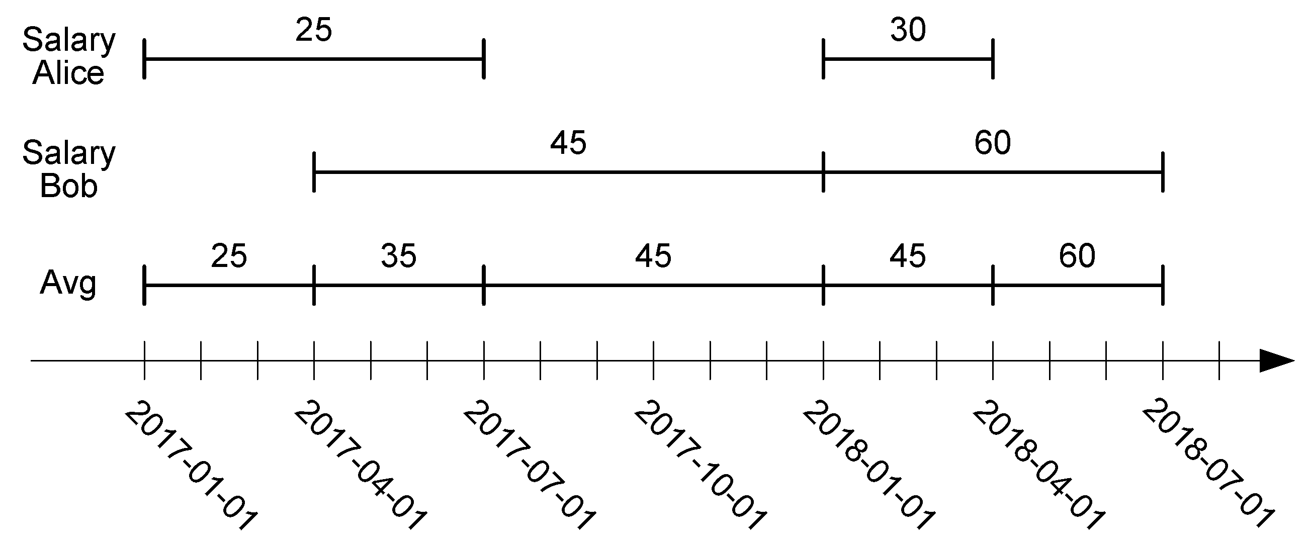
Note that when Alice’s salary is undefined, no comparison is performed. As an example of lifted aggregation, the next query asks for the average salary across time.
SELECT AVG(E.SalaryHist)
FROM  Employee E
returns
{[25@2017-01-01, 25@2017-04-01), [35@2017-04-01, 35@2017-07-01),
             [45@2017-07-01, 45@2018-04-01), [60@2018-04-01, 60@2018-07-01)}
Figure 2 shows this result graphically.
To conclude, the next example illustrates how temporal point types can be used. Consider the following table, which stores the routes followed by trucks to deliver products.
CREATE TABLE Delivery (
             TruckId CHAR(6) PRIMARY KEY,
             DeliveryDate DATE,
             Route TGEOMPOINT )
Next, two tuples are inserted in this table, containing information of two deliveries performed by two trucks T1 and T2 during the same day (as depicted in Figure 3):
INSERT INTO Delivery VALUES
( ‘T1’, ‘2017-01-10’,
                    TGEOMPOINT ‘[Point(3 3)@2017-01-10 08:00, Point(0 0)@2017-01-10 08:15]’ ),
( ‘T2’, ‘2017-01-10’,
                    TGEOMPOINT ‘[Point(4 0)@2017-01-10 08:05, Point(1 3)@2017-01-10 08:20]’ );
The routes represent continuous trajectories. Therefore, a constant speed between any two consecutive points is assumed, and linear interpolation for determining the position of the trucks at any instant is used. Examples of lifted spatial operations are given next.
The following query computes the distance between the two trucks at any time instant.
SELECT    Distance(D1.Route, D2.Route)
FROM      Delivery D1, Delivery D2
WHERE    D1.TruckId = ’T1’ AND D2.TruckId = ’T2’
This query returns the temporal float depicted in Figure 4 as follows:
[2.82842712474619@2017-01-10 08:05:00, 2@2017-01-10 08:10:00,
            2.82842712474619@2017-01-10 08:15:00]
Finally, the following query uses the lifted TIntersects topological operation for testing whether or not the two trucks intersect, as follows:
SELECT    tintersects(D1.Route, D2.Route)
FROM      Delivery D1, Delivery D2
WHERE    D1.TruckId = ‘T1’ AND D2.TruckId = ‘T2’
and the result will be
[false@2017-01-10 08:05:00, false@2017-01-10 08:15:00]
4. Modeling Mobility Data Warehouses
This section studies how DWs can be extended with temporal types in order to support the analysis of mobility data. The well-known Northwind case study is used in order to introduce the main concepts. First, basic concepts about DW modeling are introduced to make this paper self-contained.
4.1. A Short Introduction to Conceptual Modeling of Data Warehouses
The conventional database design process includes the creation of database schemas at the conceptual, logical, and physical levels. Typically, databases are designed at the conceptual level using some variation of the well-known entity-relationship (ER) model, since it has been acknowledged that conceptual models allow better communication between designers and users for the purpose of understanding application requirements.
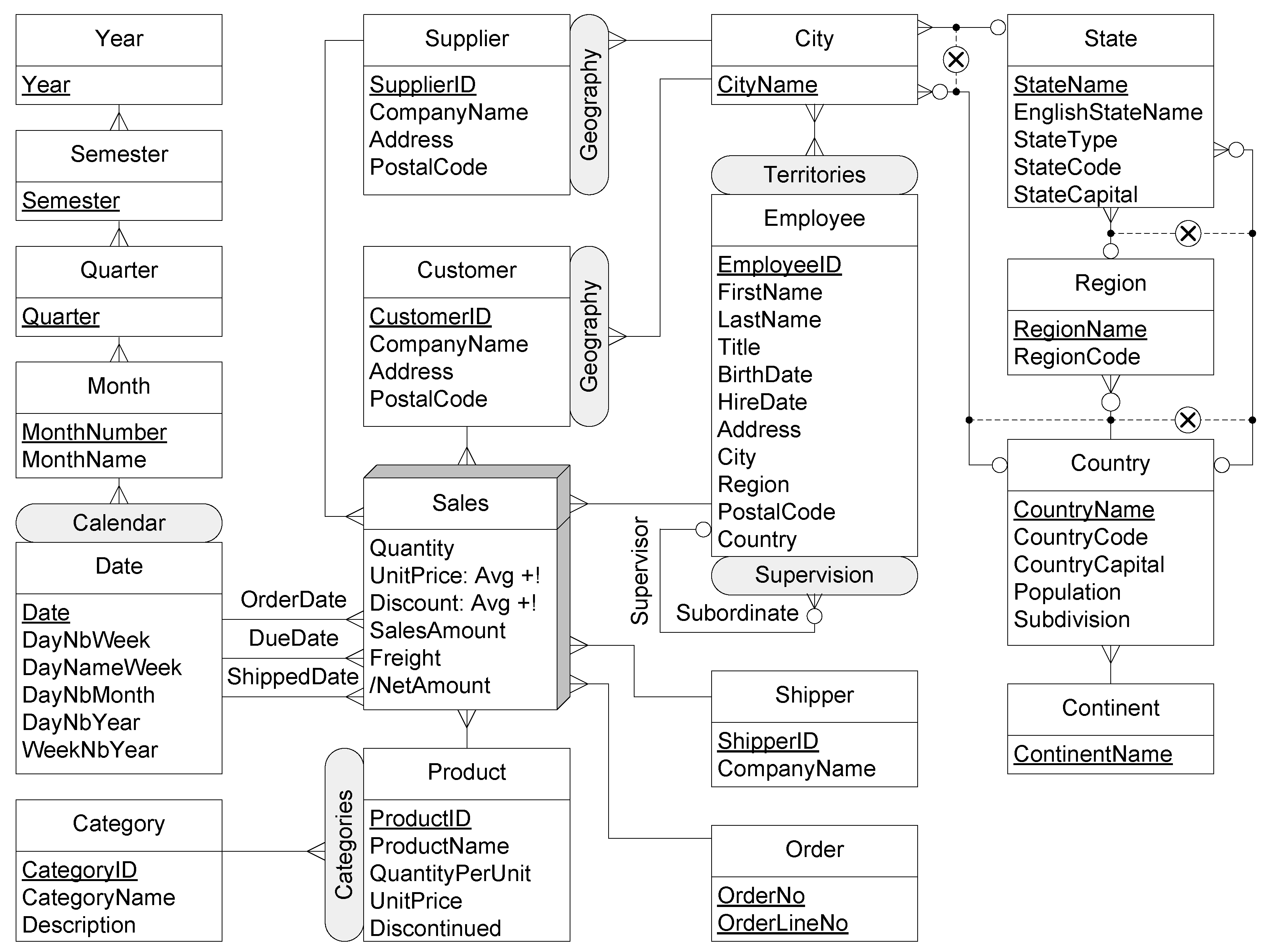
Opposite to conventional databases, there is no widely accepted conceptual model for multidimensional data. As a consequence, DW design is usually at the logical level, based on star and/or snowflake schemas [3], which are less intuitive for the final user. The present paper adopts the MultiDim model [8] to represent, at the conceptual level all elements required in DW and OLAP applications, that is, dimensions, hierarchies, and facts with their associated measures. The main reason to adopt this model is that it has also been extended to support spatial data. A streamlined description of the main components of the model follows, based on Figure 5, which represents a DW for the well-known Northwind database.
A schema is composed of a set of dimensions and a set of facts. A dimension consists of either one level, or one or more hierarchies, and a hierarchy is in turn composed of a set of levels. Instances of a level are called members. For example, Product and Category are levels in Figure 5. As shown in the figure, a level has a set of associated attributes that describe the characteristics of their members, and has one or more identifiers that uniquely identify their members. For example, in Figure 5, CategoryID is an identifier of the Category level. Each attribute of a level has a type, that is, a domain for its values (typically, integer, real, and string). For each pair of levels in a hierarchy, the lower level is called the child and the higher level is called the parent. The relationships composing of hierarchies are called parent-child relationships. The cardinalities of parent-child relationships indicate the minimum and the maximum number of members in one level that can be related to a member in another level. For example, in Figure 5 there is a one-to-many relationship between the child level Product and the parent level Category. Finally, it is sometimes the case that two or more parent-child relationships are exclusive. This is represented using the symbol ‘⊗’. This is shown in Figure 5, where states can be aggregated either into regions or into countries. Thus, according to their type, states participate in only one of the relationships departing from the State level.
A fact relates several levels. For example, the Sales fact in Figure 5 relates the Employee, Customer, Supplier, Shipper, Order, Product, and Date levels. The same level can participate several times in a fact, playing different roles such that each role is represented by a separate link between the level and the fact. For example, in Figure 5 the Date level participates in the Sales fact with the roles OrderDate, DueDate, and ShippedDate. Instances of a fact are called fact members. The cardinality of the relationship between facts and levels, indicates the minimum and the maximum number of fact members that can be related to level members. For example, in Figure 5 there is a one-to-many relationship between Sales and Product. A fact may contain (usually numeric) attributes commonly called measures, that are analyzed using the context provided by the dimensions. For example, the Sales fact in Figure 5 includes the measures Quantity, UnitPrice, Discount, SalesAmount, Freight, and NetAmount. Levels in a hierarchy are used to analyze factual data at various granularities, or levels of detail. In OLAP, this operation is called Roll-up, and aggregates measures along dimension hierarchies, up to a dimension level, using an aggregate function. The aggregation function associated with a measure can be specified next to the measure name, and the SUM aggregation function is assumed by default.
4.2. Conceptual Modeling of Mobility Data Warehouses
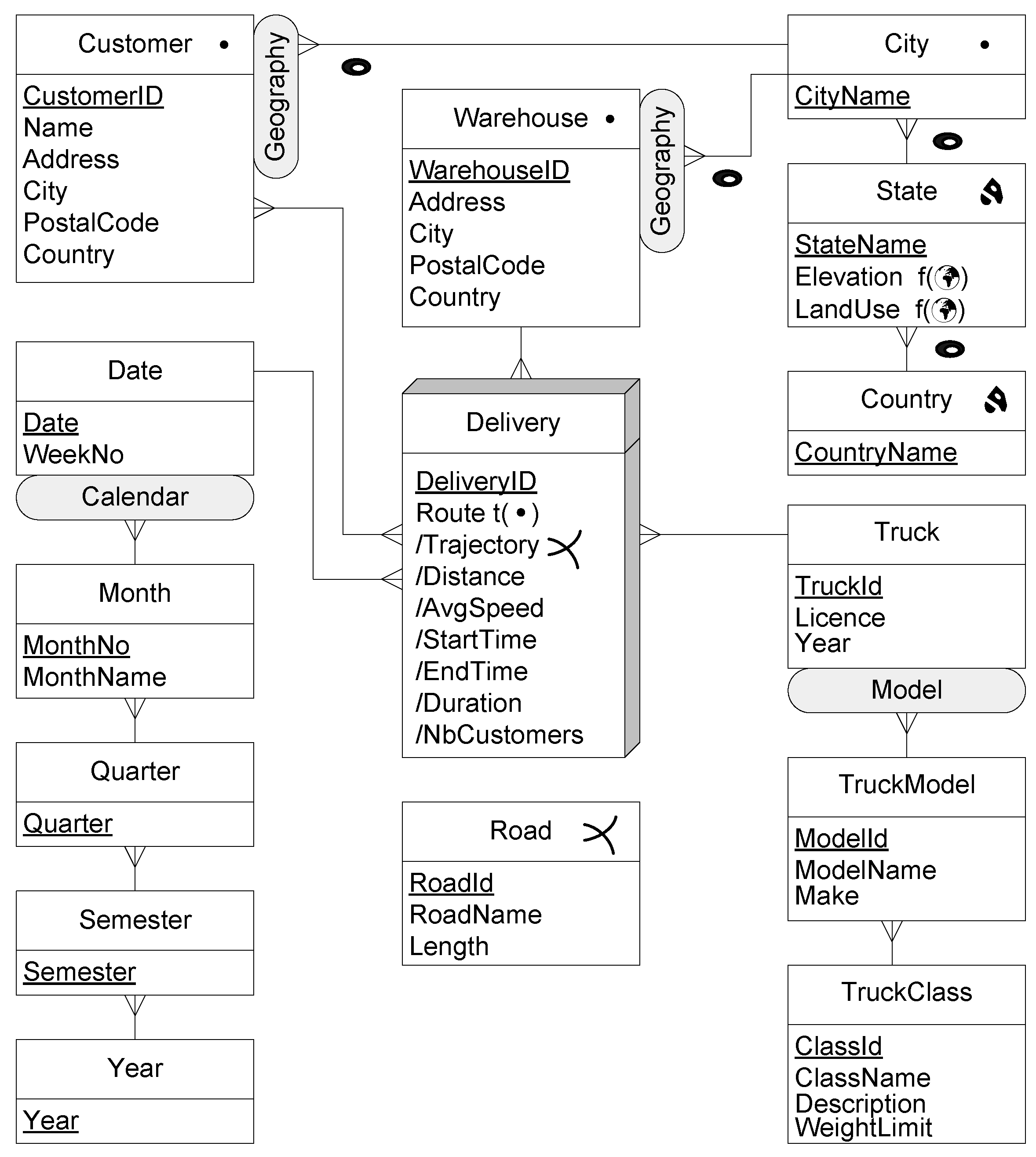
The extension of the Northwind DW to support mobility analysis is depicted in Figure 6 and explained below. The idea is aimed at building a mobility DW that keeps track of the deliveries of goods to their customers. In the company there is a fleet of trucks that load the goods in a warehouse (there are several of them), perform a delivery visiting the customers according to a delivery plan, and then return to the warehouse. There is nonspatial data about the customers, the trucks, and the warehouses that store the goods to be delivered to customers. There is also spatial data about the road network (more on this, below). Further, the geographic hierarchies are also represented as spatial data. In addition, there are the trajectories followed by the trucks (derived as a projection of the deliveries). Figure 6 shows the conceptual schema depicting this scenario using the MultiDim model extended to support spatial data and temporal types. This is explained in more detail next.
As shown in the figure, the fact Delivery is related to four dimensions: Truck, Date, Warehouse, and Customer, where the latter is related to the fact through a many-to-many relationship. The Customer dimension is composed of four levels, with a one-to-many parent-child relationship defined between each pair of levels. The level Truck has attributes TruckId, Licence, and Year. Spatial levels or attributes have an associated geometry (e.g., point, line, or region), which is indicated by a pictogram. In the example, dimensions Customer and Warehouse are spatial and share a Geography hierarchy where a geometry is associated with each level in both dimensions. Also, the State level includes to continuous fields (raster) attributes, namely LandUse and Elevation, which indicate, at each point, its land use (e.g., residential, industrial) and altitude, respectively. Finally, topological constraints are represented using pictograms in parent-child relationships. For example, the topological constraints in dimension Geography indicate that a city is contained in its parent state and similarly for the other parent-child relationships in the hierarchy.
The fact Delivery has an identifier DeliveryID, and eight measures. The first one, Route, keeps the position of the truck at any point in time. It is a spatiotemporal measure of type temporal point, as indicated by the symbol ‘t(•)’. The other measures are derived from Route. Measure Trajectory stores the geometry of the route traversed by the truck, which is a line, without any temporal information. Measures AvgSpeed, Duration, and NbCustomers are numeric, while StartTime and EndTime are timestamps.
In the example of Figure 6, the movement track of the deliveries is represented as a temporal point. In other words, the trajectory is a measure of this fact, allowing deliveries to be aggregated along the different dimensions. Another use of trajectory aggregation identifies “similar” trajectories and merges them in a single class. Thus, queries like “give me the total number of trajectories by class,” or “List all the trajectories similar to the one followed by truck T1 on 25 November 2018” are possible.
Finally, note that the road network is not linked to any fact or dimension in the schema. This is a major difference with respect to other approaches that segment trajectories, and link trajectory segments to road segments.
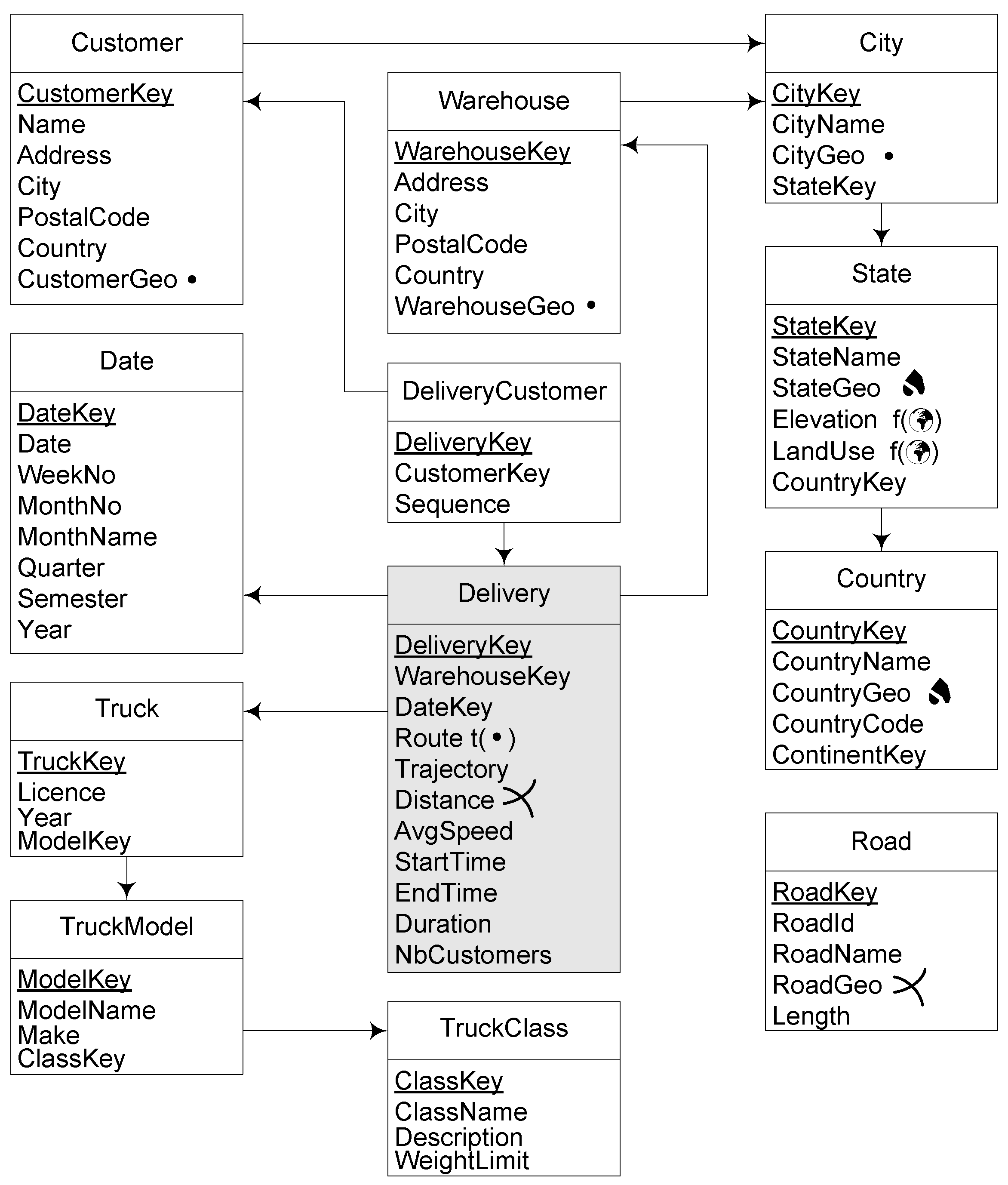
The translation of the conceptual schema in Figure 6 into a snowflake schema is shown in Figure 7. The many-to-many relationship between the Delivery fact and the Customer dimension is represented in table DeliveryCustomer, which contains the keys of the tables Delivery and Customer and the attribute Sequence, which states the order in which the customer were visited. The rest of the translation is straightforward, and it is omitted for the sake of brevity.
5. Querying the Mobility Data Warehouse in SQL and MobilityDB
In order to express queries to the Northwind mobility DW, the temporal types and their associated operations as defined in Section 3 are used. The mobility DW depicted in Figure 7 is used as an example. Queries were targeted for Belgium, in which the administrative divisions corresponding to states are called provinces. In what follows, the functions that are prefixed by ST_ are PostGIS functions, while the functions not prefixed (e.g., length) are the temporal extensions from MobilityDB. The queries below are aimed at highlighting the advantages of defining MO data as a measure rather than the typical solution of defining static segments of trajectories as measures [5,6,7]. Therefore, the queries combine typical OLAP operations, like Roll-up, Slice, and Dice, with operations on MOs (in this case, the trucks that perform the deliveries. For each query, the operations involved are explained, to remark the wide variety of queries that the model and implementation allow.
Query 1
(Roll-up + slice + distance). List the total distance traveled by trucks, per make and month.
This query involves aggregation along the Date and Truck dimensions, slicing out all other dimensions, and the computation of the distance travelled by the MOs.
SELECT M.Make, DT.Year, DT.MonthNumber, SUM(length(D.Route))FROM Delivery D, Truck T, TruckModel M, Date DTWHERE D.TruckKey = T.TruckKey AND T.ModelKey = M.ModelKey ANDD.DateKey = DT.DateKeyGROUP BY M.Make, DT.Year, DT.MonthNumberORDER BY M.Make, DT.Year, DT.MonthNumberAlso, the query uses the function length to compute the distance traveled by each delivery, and then aggregates the distances per truck make and month in the usual way.
An analysis of this query makes it clear the advantage of the approach presented here, with respect to the approaches that segment the trajectories in order to provide a relational representation of a trajectory. The latter would require, for example, to compute the length of each segment individually (see [8], Chapter 12, for a detailed explanation), and also joining each segment with other dimension tables. Further, proposals that partition the space into a grid, precomputing aggregated measures for each cell in the grid (see Section 6), of course cannot express this query, neither any of the queries in the next examples. Also, even though MO databases like Secondo and Hermes (also see Section 6) could of course address the MO part of the queries, integrating them into a system to perform OLAP operations is far from being trivial. Therefore, it can be seen that the mobility DW approach based on MobilityDB takes the best of both worlds, bridging the gap between them. The explanation above applies to all queries that are discussed below in this section, thus, it will not be repeated to avoid redundancy.
Query 2
(Roll-up + slice + dice + duration). List the average duration per day of deliveries starting with a customer located in the province of Namur.
This query requires aggregation along the Date dimension, a Roll-up operation over the Customer dimension, a Dice operation to select the province of Namur at the State level, and the computation of the duration of the time spanned by the deliveries. Finally, all dimensions but Date are sliced out.
              SELECT         DT.Date, AVG(duration(D.Route))
              FROM          Delivery D, DeliveryCustomer DC, Customer C, State S, Date DT
              WHERE        D.DeliveryKey = DC.DeliveryKey AND DC.Sequence = 1 AND
              DC.CustomerKey = C.CustomerKey AND C.StateKey = S.StateKey AND
              S.Name = ’Namur’ AND D.DateKey = DT.DateKey
              GROUP BY DT.Date
              ORDER BY DT.Date
The query selects the first customer visited by a delivery using the attribute Sequence, and verifies that she is located in the province of Namur. Then, it uses function duration to compute the duration of the delivery. Finally, the query computes the average of the durations per day.
Query 3
(Roll-up + slice + dice + spatial + duration). For each month, compute the number of deliveries such that their route intersects the province of Namur for more than 20 min.
The query performs a roll-up operation along the Date and Customer dimensions, a Dice operation to select the province of Namur at the State level, a spatial operation to compute the intersection, and the computation of the duration of the time spanned by the deliveries within the province. Finally, all dimensions but Date are sliced out.
              SELECT        T.Year, T.MonthNumber, COUNT(*)
              FROM         Delivery D, Date T, State S
              WHERE       D.DateKey = T.DateKey AND S.Name = ’Namur’ AND D.Route && S.Geom AND
              duration(atGeometry(D.Route, S.Geom)) >= interval ’20 min’
              GROUP BY T.Year, T.MonthNumber
              ORDER BY T.Year, T.MonthNumber
This query uses the function atGeometry to restrict the route of the delivery to the geometry of the province of Namur. Then, function duration computes the time spent within the province and verifies that this duration is at least of 20 min. Remark that this duration of 20 min may not be continuous. Finally, the count of the selected deliveries is performed as usual.
The term D.Route && S.Geom is optional and it is included to enhance query performance. It verifies, using an index, that the spatio-temporal bounding box of the delivery projected over the spatial dimension intersects with the bounding box of the geometry. In this way, the atGeometry function is only applied to the deliveries satisfying the bounding box condition.
Query 4
(Roll-up + slice + dice + spatial + duration). Same as the previous query but with the condition that the route intersects the province of Namur for more than consecutive 20 min.
The operations involved here are similar to the ones in the previous query. The queries differ in the way in which they compute the duration. Again, this is only possible when measures are actually represented as MOs.
              SELECT        DT.Year, DT.MonthNumber, COUNT(*)
              FROM         Delivery D, Date DT, State S,
              unnest(periods(getTime(atGeometry(D.Route, S.Geom)))) P
              WHERE       D.DateKey = DT.DateKey AND S.Name = ’Namur’ AND
              D.Route && S.Geom AND duration(P) >= interval ’20 min’
              GROUP BY DT.Year, DT.MonthNumber
              ORDER BY DT.Year, DT.MonthNumber
As in the previous query, the function atGeometry restricts the route of the delivery to the province of Namur. This results in a route that may be discontinuous in time, because the route may enter and leave the province. The query uses the function getTime to obtain the set of periods of the restricted delivery, represented as a periodSet value. The function periods converts the latter value into an array of periods, and the PostgreSQL function unnest expands this array to a set of rows, each row containing a period P. Then, it is possible to verify that the duration of one of the periods P has at least 20 min.
Query 5
(Roll-up + slice + distance + speed). For each month, compute the total number of deliveries that traveled at least 50 km at a speed higher than 100 km/h.
The operations involved in this query are: a Roll-up along the Date dimension, and the computation of the distance and speed functions on the MO data. Finally, slicing is performed to drop all dimensions but Date.
              SELECT        DT.Year, DT.MonthNumber, COUNT(*)
              FROM         Delivery D, Date DT
              WHERE       D.DateKey = DT.DateKey AND length(atPeriodSet(D.Route,
              getTime(atRange(speed(Route) * 3.6, ’[100,infinity]’)))) / 1000 > 50
              GROUP BY DT.Year, DT.MonthNumber
              ORDER BY DT.Year, DT.MonthNumber
The query uses the function speed to obtain a temporal float representing the speed of the route at each instant, expressed in units per second, depending on the spatial reference system, which in our case is meters per second. This temporal value is then transformed into kilometers per hour by multiplying it by 3.6. The function atRange restricts the speed to the float range [100, infinity]. The getTime function computes the set of periods during which the delivery travels at more than 100 km/h. The function atPeriodSet restricts the delivery to these periods and the length function computes the distance traveled by the restricted deliveries, expressed in meters, which is then converted to kilometers and compared against the value 50.
Query 6
(Temporal aggregation). For each speed range of 20 km/h, give the total distance traveled by all trucks within that range.
This is a typical temporal aggregation query, as explained below. That is, operations over MOs are performed over the measure, without involving the dimensions. Only the fact table is used here.
              WITH Ranges AS (
              SELECT I AS RangeID, floatrange(((I-1)*20), I*20) AS Range
              FROM generate_series(1,10) I )
              SELECT       R.Range, SUM(length(atPeriodSet(D.Route,
              getTime(atRange(speed(D.Route) * 3.6, R.Range)))) / 1000)
              FROM        Delivery D, Ranges R
              WHERE      atRange(speed(D.Route) * 3.6, R.Range) IS NOT NULL
              GROUP BY R.RangeID, R.Range
              ORDER BY R.RangeID
This idea of this query is to allow having an overall view of the speed behaviour of the entire fleet of delivery trucks. The temporary table Ranges stores the ranges , , …. In the main query, the speed of the route, obtained in meters per second, is transformed into kilometers per hour. Then, the function atRange restricts the route to the portions having a given speed range. The time periods comprising the restricted route are obtained with the getTime function. The overall route is restricted then to the obtained time periods with the function atPeriodSet, the distance traveled at the given speed range is obtained with the length function, and all the distances for all trucks at the given time range are obtained with the SUM aggregation function.
Query 7
(Slice + spatial). Compute the number of deliveries that traversed at least two states.
The OLAP operation here is a Slice, to drop all dimensions. The rest of the query involves spatial operations to perform intersections between the MOs’ trajectories and the State dimension level. Note that, in fact, the intersection is performing a “climbing” along the geographic dimension, skipping the intermediate levels in the hierarchy.
              SELECT      COUNT(*)
              FROM        Delivery D, State S1, State S2
              WHERE      S1.StakeyKey <> S2.StateKey AND
              ST_Intersects(trajectory(D.Route), S1.Geom) AND
              ST_Intersects(trajectory(D.Route), S2.Geom)
This query projects the route of the delivery to the spatial dimension using the function trajectory, which results in a geometry. The query then tests that the trajectory of the route intersects two states using the PostGIS function ST_Intersects.
Query 8
(Slice + distance + duration). List the pairs of deliveries that traveled at less than one kilometer from each other during more than half an hour. Again, the OLAP operation here is a Slice, to drop all dimensions. Only the Delivery fact is kept. Then, computations on the temporal types are performed.
              SELECT        D1.DeliveryKey, D2.DeliveryKey
              FROM         Delivery D1, Delivery D2
              WHERE       D1.DeliveryKey <> D2.DeliveryKey AND duration(getTime(
              atValue(tdwithin(D1.Route, D2.Route, 1000), TRUE))) > ‘20 min’
The function tdwithin is the temporal version of the PostGIS function ST_DWithin. It returns a temporal boolean which is true during the periods when the two routes are within the specified distance from each other. The function atValue restricts the temporal boolean to the periods when its value is true, and the function getTime obtains these periods. Finally, the query uses the duration function to obtain the corresponding interval and verifies that it is greater than 20 min.
The next example query involves the LandUse continuous field.
Query 9
(Roll-up + slice + spatial (raster) + distance + duration). Compute the average duration of the deliveries that started in a residential area and ended in an industrial area on 1 February 2017.
The OLAP operations are a slice, to drop all dimensions but Date and Customer, and a roll-up over the Customer (only up to the bottom level) and Date dimensions. Spatial operations over raster data are also performed. Finally, also computations on the temporal types are performed.
              SELECT AVG(duration(D.Route))
              FROM   Delivery D, Date T, DeliveryCustomer DC1, DeliveryCustomer DC2,
              Customer C1, Customer C2, City Y1, City Y2, State S1, State S2
              WHERE D.DateKey = T.DateKey AND D.Date = ’2017-02-01’ AND
              D.DeliveryKey = DC1.DeliveryKey AND DC1.Sequence = 1 AND
              D.DeliveryKey = DC2.DeliveryKey AND DC2.Sequence = D.NbCustomers AND
              DC1.CustomerKey = C1.CustomerKey AND
              DC2.CustomerKey = C2.CustomerKey AND
              C1.CityKey = Y1.CityKey AND C2.CityKey = Y2.CityKey AND
              Y1.StateKey = S1.StateKey AND Y2.StateKey = S2.StateKey AND
              ST_Intersects(C1.CustomerGeo,AtValue(S1.LandUse, ’Residential’)) AND
              ST_Intersects(C2.CustomerGeo,AtValue(S2.LandUse, ’Industrial’))
The query starts by selecting the deliveries of the given date. It also selects, using the bridge table DeliveryCustomer, the first and last customers served by the delivery. Then, the query obtains the state of these customers with the subsequent joins. Further, the function AtValue restricts the land use fields of the corresponding states to the values of type residential or industrial. Finally, the function ST_Intersects ensures that the start and end locations of the delivery are included in the restricted fields. Notice that, in PostGIS, the ST_Intersects predicate can compute not only if two geometries intersect, but also if a geometry and a raster intersect.
Note that the query above does not involve temporal data since it neither mentions a temporal geometry such as measure Route, nor a temporal field such as Temperature. The next query involves both temporal attributes, and combines a field and a trajectory.
Query 10
(Slice + spatial (raster) + distance). List the deliveries that have traveled along more than 50 km of roads at more than 1000 m of altitude.
A slice is performed to drop all dimensions. Spatial operations over raster data (in this case, representing elevation) are performed. Finally, computations on the temporal types are also performed.
              SELECT     D.DeliveryNumber
              FROM       Delivery D
              WHERE     ( SELECT  SUM(ST_Length(ST_Intersection(Trajectory(D.Route),
              AtRange(S.Elevation, ’[1000,infinity)’)).geom))
              FROM     State S
              WHERE   ST_Intersects(Trajectory(D.Route), S.StateGeo) ) > 50,000
For each delivery, using the function ST_Intersects, the inner query verifies that the route of the delivery and the geometry of the state intersect. Then, the elevation field of the state is restricted to the range of values higher than 1000 m with function AtRange. The function ST_Intersection computes the intersection of the trajectory of the route and the restricted field, and the length of this route is computed with the function ST_Length. The SUM aggregate function is then used to calculate the sum of the lengths of all the obtained routes for all states, and finally the outer query verifies that this sum is greater than 50 km.
Discussion on Performance
Since the paper is oriented to show the features of the mobility data warehousing approach, it is focused on highlighting the expressiveness that MO data adds to the classic and spatial data warehousing approaches. Therefore, a thorough evaluation of query performance is outside the scope of this work. Nevertheless, this section reports a preliminary evaluation, developed as follows. The mobility DW depicted in Figure 7 was implemented over a PostgresSQL relational database. Delivery data (the MO data in attribute Route of the fact table Delivery) had been produced using the data generator of the BerlinMOD benchmark for moving objects http://dna.fernuni-hagen.de/secondo/BerlinMOD/BerlinMOD.html. However, since the BerlinMOD benchmark targets the city of Berlin, the geographic hierarchy has been dropped, and the references to the State dimension had been replaced by a Borough dimension, both in the schema and in the queries. The evaluation was performed with 520 delivery tuples. The minimum, maximum, and average length of the deliveries are 96, 4632, and 1870, respectively, therefore, this would be approximately equivalent in size to a “normalized” fact table of one million records. There rest of the data are based on the Northwind database. Thus, the table Customer contains 1430 tuples, and there are seven warehouses and 100 trucks. Queries 1–8 were run (Queries 9 and 10 were not run, since they include raster data just as an example), changing, as mentioned, the references to the State with references to the Borough. For example, Query 3 now reads:
SELECT      T.Year, T.MonthNumber, COUNT(*)
FROM        Delivery D, Date T, Borough B
WHERE      D.DateKey = T.DateKey AND S.Name = ’Mitte’ AND D.Route && B.Geom AND
                  duration(atGeometry(D.Route, B.Geom)) >= interval ’20 min’
GROUP BY T.Year, T.MonthNumber
ORDER BY T.Year, T.MonthNumber
Analogously, Query 4 reads, for these experiments:
SELECT      DT.Year, DT.MonthNumber, COUNT(*)
FROM        Delivery D, Date DT, Borough B,
                  unnest(periods(getTime(atGeometry(D.Route, B.Geom)))) P
WHERE      D.DateKey = DT.DateKey AND B.Name = ’Mitte’ AND
                  D.Route && B.Geom AND duration(P) >= interval ’20 min’
GROUP BY DT.Year, DT.MonthNumber
ORDER BY DT.Year, DT.MonthNumber
Table 1 shows the results obtained in these tests. Queries were run several times to eliminate the influence of cold caching (that is, hot chache is assumed). Further, once this influence was eliminated, execution times were the same for each run, therefore just the average value was reported in the table, since the differences between runs were negligible. It can be seen that the queries that took longer were the ones that included spatial operations.
Of course, these results are not pretended to be conclusive, but suggest that the addition of MOs as fact measures in a warehouse adds query expressiveness. Also, existing proposals segment trajectories (see Section 6) require a “normalization” of the trajectory representation, which is costly due to the number of joins that queries like the ones presented here would require. This is not needed when trajectories are represented as MOs. In addition, note that the DW is implemented using standard object-relational technologies (in this case, PostgresSQL and PostGIS). Therefore, the effect of the inclusion of MOs can also be inferred from an evaluation of the implementation of the temporal types. This is available in the MobilityDB demo site, at URL http://demo.mobilitydb.eu/, where the system runs over the BerlinMOD benchmark data (the queries in such demo do not include warehouse data, they are purely MO queries). It can be observed on the demo site that typical MO queries run very fast over the benchmark, although this is not reported in this paper. Developing a benchmark to perform a comprehensive set of experiments is outside the scope of this paper, and is planned as future work (Section 7).
6. Related Work
Trajectory DWs are strongly related to spatial databases and DWs. The main features of PostGIS, the OGC-based extension to PostgresSQL can be found in [12]. Also, the spatial extension of the MultiDim model presented here was based on the spatial data types of MADS [13], a spatiotemporal conceptual model. The notion of spatial OLAP (SOLAP) was introduced in [14], and it is reviewed in [15]. Other relevant work on SOLAP can be found in [16,17,18].
In order to support spatio-temporal data, a data model and associated query language for MO data were needed. This is achieved in Secondo http://dna.fernuni-hagen.de/secondo/ [19], a MO database system developed at the FernUniversität in Hagen, based on the model of Güting et al. [1]. Along similar lines, Hermes is a MOD introduced by Pelekis et al. [20]. The Hermes system is described in [21]. In spite of their ability to handle MO data, neither Secondo, nor Hermes, are oriented toward addressing the problem of mobility DWs. Among other reasons, integrating both prototypes into existing relational databases is not straightforward. Hermes, for example, extends Oracle through a so-called cartridge with the MO types. However, to build an application on top of the database the application developer must write a source program (for example, in Java), and embed PL/SQL scripts that invoke object constructors and methods from Hermes. Secondo is as packed system, therefore, integration with existing databases is even more complicated. On the contrary, being coded in the “C” programming language (like PostgresSQL), MobilityDB seamlessly extends the PostGIS library with temporal data types, not requiring any additional software architecture. Thus, building a mobility DW with MobilityDB turns out to be a natural extension of a spatial relational DW. On the downside, MobilityDB at this time only supports moving points, while Secondo and Hermes provide (although limited) support to other MOs. However, for traffic analysis, moving points are the most used kind of MOs. The data type system of the temporal types presented in this paper follows the approach of [1]. Also, an SQL extension for spatiotemporal data is proposed in [22].
The work by Orlando et al. [6] introduces the concept of trajectory DWs, aimed at providing the infrastructure needed to deliver advanced reporting capabilities and facilitating the use of mining algorithms on aggregate data. This work is based on the Hermes system. A relevant feature of this proposal is the treatment given to the extraction, transformation and loading (ETL) process, which transforms the raw location data and loads it to the trajectory DW. However, regarding mobility analysis, this proposal does not address MO data. Measures in this trajectory DW are related with the number of MO present in a cell defined by spatiotemporal coordinates. Therefore, queries that can be addressed using this DW are of the form “compute the number of cars between latitudes and , and longitudes and , on 3 November 2018”. However, actual mobility analysis queries like the ones presented in Section 5 cannot be addressed. Also, the authors themselves state in their proposal that MO data analysis remains outside the TDW.
Along similar lines, Wagner et al. [7] proposed the Mob-Warehouse, a conceptual to support mobility analysis using a TDW. The authors propose to enrich trajectory data with semantic information about the domain. The paper is based on the previously defined notion of semantic trajectory [23]. Unlike the model presented in [6], where the measures are pre-aggregated (e.g., number of cars in a cell), in this model the measures are at the finest detail level. No implementation details are given, and MO operations are not addressed. Instead, the proposal is aimed at analyzing semantic trajectories, as the example queries provided suggest.
Based on [7,23], and the work on semantic trajectories, another model for TDWs is proposed in [5], accounting for semantic information. In this case, again, MO data are only partially considered. MO trajectories are partitioned into segments, to which semantic information is associated. No implementation is described, and the authors report than experiments are being carried out, suggesting that the segments in the fact table are not that efficient, which is certainly expected given that many joins are required to reconstruct a trajectory from such segments.
Note that the proposal presented in the present paper does not exclude semantic information. On the contrary, semantic information about MOs can be naturally included in the mobility DW proposed here, and, in fact, this is what dimensions are defined for. Also, all of the features of the proposals above are supported by the model described in this paper (e.g., segmentation, pre-aggregation, semantic information).
An overall perspective of the state of the art in mobility data management can be found in [2,24,25,26]. A survey on spatiotemporal data warehousing, OLAP, and mining is given in [27]. A discussion about the meaning of spatiotemporal data warehousing is given in [4]. Also, mobility DWs are discussed in [28,29,30]. Analysis tools for mobility DWs can be found in [31]. Finally, a survey on spatiotemporal aggregation is given in [32], while a survey on trajectory aggregation is provided in [33].
7. Conclusions
This paper studied how DWs can be extended with spatial and mobility data. For this, temporal types were defined to capture the variation of a value across time. The paper discussed how these data types, representing MOs, were implemented as an extension to PostGIS. This extension allows to define a conceptual model for a trajectory DW, which includes MO data as measures that can be analyzed with respect to contextual dimensions. Therefore, the contextual model can actually be implemented with MO data, not only segmented trajectories or pre-aggregated measures. This is a key difference with previous proposals, and would not be possible without a data type system that seamlessly integrates with the (spatial) database supporting the warehouse. A concrete case study that extends the Northwind DW with mobility data was presented, illustrating the use of the mobility DW with a comprehensive set of queries. Future work includes the development of more kinds of temporal types supporting not only moving points, but also moving lines and moving regions and, as mentioned in Section 5, the development of an appropriate benchmark to allow a fair evaluation of mobility DWs. Another research direction will address the extension of the work presented in this paper, to big data environments, along the lines mentioned in Section 1.
Author Contributions
Both authors contributed equally to the writing of the paper.
Funding
This research received no external funding.
Acknowledgments
Alejandro Vaisman was partially supported by the Argentinian National Scientific Agency, PICT-2014 Project 0787, and PICT-2017 Project 1054.
Conflicts of Interest
The authors declare no conflict of interest.
References
- Güting, R.; Schneider, M. Moving Objects Databases; Morgan Kaufmann: Burlington, MA, USA, 2005. [Google Scholar]
- Renso, C.; Spaccapietra, S.; Zimányi, E. (Eds.) Mobility Data: Modeling, Management, and Understanding; Cambridge Press: Cambridge, UK, 2018. [Google Scholar]
- Kimball, R.; Ross, M. The Data Warehouse Toolkit: The Complete Guide to Dimensional Modeling, 2nd ed.; Wiley: Hoboken, NJ, USA, 2002. [Google Scholar]
- Vaisman, A.; Zimányi, E. What is spatio-temporal data warehousing? In Data Warehousing and Knowledge Discovery—Proceedings of the 11th International Conference on Data Warehousing and Knowledge Discovery, DaWaK’09, Linz, Austria, 31 August–2 September 2009; No. 5691 in Lecture Notes in Computer Science; Springer: Berlin, Germany, 2009; pp. 9–23. [Google Scholar]
- Fileto, R.; Raffaetà, A.; Roncato, A.; Sacenti, J.A.P.; May, C.; Klein, D. A Semantic Model for Movement Data Warehouses. In Proceedings of the 17th International Workshop on Data Warehousing and OLAP, Shanghai, China, 3–7 November 2014; pp. 47–56. [Google Scholar]
- Orlando, S.; Orsini, R.; Raffaetà, A.; Roncato, A.; Silvestri, C. Spatio-temporal aggregations in trajectory data warehouses. J. Comput. Sci. Eng. 2007, 1, 211–232. [Google Scholar] [CrossRef]
- Wagner, R.; de Macedo, J.A.F.; Raffaetà, A.; Renso, C.; Roncato, A.; Trasarti, R. Mob-Warehouse: A Semantic Approach for Mobility Analysis with a Trajectory Data Warehouse. In Advances in Conceptual Modeling—ER 2018 Workshops, LSAWM, MoBiD, RIGiM, SeCoGIS, WISM, DaSeM, SCME, and PhD Symposium, Hong Kong, China, 11–13 November 2018; Revised Selected Papers; Springer: Berlin, Germany, 2018; pp. 127–136. [Google Scholar]
- Vaisman, A.; Zimányi, E. Data Warehouse Systems: Design and Implementation; Springer: Berlin, Germany, 2014. [Google Scholar]
- Tansel, A.; Clifford, J.; Gadia, S.; Jajodia, J.; Segev, A.; Snodgrass, T. (Eds.) Temporal Databases: Theory, Design, and Implementation; Benjamin-Cummings: San Francisco, CA, USA, 1993. [Google Scholar]
- Güting, R.; Böhlen, M.H.; Erwig, M.; Jensen, C.S.; Lorentzos, N.A.; Schneider, M.; Vazirgiannis, M. A foundation for representing and quering moving objects. ACM Trans. Database Syst. 2000, 25, 1–42. [Google Scholar] [CrossRef]
- Gadia, S.; Nair, S. Temporal Databases: A Prelude to Parametric Data. In Temporal Databases: Theory, Design, and Implementation; Tansel, A., Clifford, J., Gadia, S., Segev, A., Snodgrass, R.T., Eds.; Benjamin-Cummings: San Francisco, CA, USA, 1993; Chapter 2; pp. 28–66. [Google Scholar]
- Obe, R.; Hsu, L. PostGIS in Action; Manning Publications Co.: Shelter Island, NY, USA, 2014. [Google Scholar]
- Parent, C.; Spaccapietra, S.; Zimányi, E. Conceptual Modeling for Traditional and Spatio-Temporal Applications: The MADS Approach; Springer: Berlin, Germany, 2006. [Google Scholar]
- Rivest, S.; Bédard, Y.; Marchand, P. Toward Better Suppport for Spatial Decision Making: Defining the Characteristics of Spatial On-Line Analytical Processing (SOLAP). Geomatica 2001, 55, 539–555. [Google Scholar]
- Bédard, Y.; Rivest, S.; Proulx, M. Spatial Online Analytical Processing (SOLAP): Concepts, Architectures, and Solutions from a Geomatics Engineering Perspective. In Data Warehouses and OLAP: Concepts, Architectures and Solutions; Wrembel, R., Koncilia, C., Eds.; IRM Press: Aarhus, Denmark, 2007; Chapter 13; pp. 298–319. [Google Scholar]
- Bimonte, S.; Bertolotto, M.; Gensel, J.; Boussaid, O. Spatial OLAP and Map Generalization: Model and Algebra. Int. J. Data Wareh. Min. 2017, 8, 24–51. [Google Scholar] [CrossRef]
- Boulil, K.; Bimonte, S.; Pinet, F. Conceptual model for spatial data cubes: A UML profile and its automatic implementation. Comput. Stand. Interfaces 2015, 38, 113–132. [Google Scholar] [CrossRef]
- Viswanathan, G.; Schneider, M. On the Requirements for User-Centric Spatial Data Warehousing and SOLAP. In Database Systems for Advanced Applications Proceedings of the DASFAA 2011 Workshops, Hong Kong, China, 22–25 April 2011; Xu, J., Yu, G., Zhou, S., Unland, R., Eds.; Lecture Notes in Computer Science; Springer: Berlin, Germany, 2011; Volume 6637, pp. 144–155. [Google Scholar]
- Xu, J.; Güting, R. A generic data model for moving objects. GeoInformatica 2018, 17, 125–172. [Google Scholar] [CrossRef]
- Pelekis, N.; Theodoridis, Y.; Vosinakis, S.; Panayiotopoulos, T. Hermes: A Framework for Location-Based Data Management. In Advances in Database Technology—EDBT 2006—Proceedings of the 10th International Conference on Extending Database Technology, Munich, Germany, 26–31 March 2006; Ioannidis, Y., Scholl, M., Schmidt, J., Eds.; No. 3896 in Lecture Notes in Computer Science; Springer: Munich, Germany, 2006; pp. 1130–1134. [Google Scholar]
- Pelekis, N.; Theodoridis, Y. Mobility Data Management and Exploration; Springer: Berlin, Germany, 2014. [Google Scholar]
- Viqueira, J.; Lorentzos, N. SQL extension for spatio-temporal data. VLDB J. 2007, 16, 179–200. [Google Scholar] [CrossRef]
- Bogorny, V.; Renso, C.; de Aquino, A.R.; de Lucca Siqueira, F.; Alvares, L.O. CONSTAnT—A Conceptual Data Model for Semantic Trajectories of Moving Objects. Trans. GIS 2014, 18, 66–88. [Google Scholar] [CrossRef]
- Meng, X.; Ding, Z.; Xu, J. Moving Objects Management: Models, Techniques and Applications, 2nd ed.; Springer: Berlin, Germany, 2014. [Google Scholar]
- Andrienko, G.; Andrienko, N.; Bak, P.; Keim, D.; Wrobel, S. Visual Analytics of Movement; Springer: Berlin, Germany, 2014. [Google Scholar]
- Zheng, Y.; Zhou, X. (Eds.) Computing with Spatial Trajectories; Springer: Berlin, Germany, 2011. [Google Scholar]
- Gómez, L.; Kuijpers, B.; Moelans, B.; Vaisman, A.A. A State-of-the-Art in Spatio-Temporal Data Warehousing, OLAP and Mining. In Integrations of Data Warehousing, Data Mining and Database Technologies: Innovative Approaches; Taniar, D., Chen, L., Eds.; IGI Global: Hershey, PA, USA, 2011; Chapter 9; pp. 200–236. [Google Scholar]
- Andersen, O.; Krogh, B.B.; Thomsen, C.; Torp, K. An Advanced Data Warehouse for Integrating Large Sets of GPS Data. In Proceedings of the 17th ACM International Workshop on Data Warehousing and OLAP, Shanghai, China, 3–7 November 2014; ACM Press: New York, NY, USA, 2014; pp. 13–22. [Google Scholar]
- Marketos, G.; Frentzos, E.; Ntoutsi, I.; Pelekis, N.; Raffaetà, A.; Theodoridis, Y. Building real-world trajectory warehouses. In Proceedings of the 7th ACM International Workshop on Data Engineering for Wireless and Mobile Access, Vancouver, BC, Canada, 13 June 2008; ACM Press: New York, NY, USA, 2008; pp. 8–15. [Google Scholar]
- Pelekis, N.; Raffaetà, A.; Damiani, M.-L.; Vangenot, C.; Marketos, C.; Frentzos, E.; Ntoutsi, I.; Theodoridis, Y. Towards trajectory data warehouses. In Mobility, Data Mining and Privacy: Geographic Knowledge Discovery; Giannotti, F., Pedreschi, D., Eds.; Springer: Berlin, Germany, 2008; Chapter 9; pp. 189–211. [Google Scholar]
- Raffaetà, A.; Leonardi, L.; Marketos, G.; Andrienko, G.; Andrienko, N.V.; Frentzos, E.; Giatrakos, N.; Orlando, S.; Pelekis, N.; Roncato, A.; et al. Visual mobility analysis using T-Warehouse. Int. J. Data Wareh. Min. 2011, 7, 1–23. [Google Scholar] [CrossRef]
- Vega López, I.; Snodgrass, R.; Moon, B. Spatiotemporal Aggregate Computation: A survey. IEEE Trans. Knowl. Data Eng. 2005, 17, 271–286. [Google Scholar] [CrossRef]
- Andrienko, G.; Andrienko, N. A general framework for using aggregation in visual exploration of movement data. Cartogr. J. 2010, 47, 22–40. [Google Scholar] [CrossRef]
Figure 1.
Representation of the evolution of salaries of two employees using the type temporal(integer).
Figure 1.
Representation of the evolution of salaries of two employees using the type temporal(integer).

Figure 2.
Example of the temporal average operation.

Figure 3.
Trajectories of two trucks as a projection of a temporal point into the plane.

Figure 4.
Distance between the trajectories of the two trucks in Figure 3 represented as a temporal(real).
Figure 4.
Distance between the trajectories of the two trucks in Figure 3 represented as a temporal(real).

Figure 5.
Conceptual schema of the Northwind data warehouse.

Figure 6.
Conceptual schema of the Northwind mobility data warehouse.

Figure 7.
Logical schema of the Northwind mobility data warehouse.


Table 1.
Running queries.
| Query | Execution Time (s) |
|---|---|
| Q1 | 2 |
| Q2 | 0.35 |
| Q3 | 180 |
| Q4 | 180 |
| Q5 | 12 |
| Q6 | 60 |
| Q7 | 60 |
| Q8 | 9 |
© 2019 by the authors. Licensee MDPI, Basel, Switzerland. This article is an open access article distributed under the terms and conditions of the Creative Commons Attribution (CC BY) license (http://creativecommons.org/licenses/by/4.0/).
Share and Cite
MDPI and ACS Style
Vaisman, A.; Zimányi, E. Mobility Data Warehouses. ISPRS Int. J. Geo-Inf. 2019, 8, 170. https://doi.org/10.3390/ijgi8040170
AMA Style
Vaisman A, Zimányi E. Mobility Data Warehouses. ISPRS International Journal of Geo-Information. 2019; 8(4):170. https://doi.org/10.3390/ijgi8040170
Chicago/Turabian StyleVaisman, Alejandro, and Esteban Zimányi. 2019. "Mobility Data Warehouses" ISPRS International Journal of Geo-Information 8, no. 4: 170. https://doi.org/10.3390/ijgi8040170
Note that from the first issue of 2016, this journal uses article numbers instead of page numbers. See further details here.