A High Throughput Hardware Architecture for Parallel Recursive Systematic Convolutional Encoders

Abstract

During the last years, recursive systematic convolutional (RSC) encoders have found application in modern telecommunication systems to reduce the bit error rate (BER). In view of the necessity of increasing the throughput of such applications, several approaches using hardware implementations of RSC encoders were explored. In this paper, we propose a hardware intellectual property (IP) for high throughput RSC encoders. The IP core exploits a methodology based on the ABCD matrices model which permits to increase the number of inputs bits processed in parallel. Through an analysis of the proposed network topology and by exploiting data relative to the implementation on Zynq 7000 xc7z010clg400-1 field programmable gate array (FPGA), an estimation of the dependency of the input data rate and of the source occupation on the parallelism degree is performed. Such analysis, together with the BER curves, provides a description of the principal merit parameters of a RSC encoder.

1. Introduction

During the last years, many applications, like space telecommunications systems [1], digital TV broadcasting [2] and wireless metropolitan area networks [3] have been exploiting forward error correcting (FEC) codes to reduce the bit error rate (BER) in data transmission. FEC approaches encode data to transmit by using redundant codes which allow to estimate the correct bit stream transmitted at receiver by using a maximum likelihood [4] or a maximum a posteriori [5] decoding. One of the most important FEC techniques is represented by recursive systematic convolutional (RSC) encoders. The latter are exploited as fundamental building block for the realization of more complex and efficient FECs encoders, like convolutional turbo codes (CTC) [6], which are realized by stacking RSC encoders in a parallel [7] or serial [8] configuration. In the last decades, CTCs have been the object of interest thanks to their high efficiency, which permits to transmit by using a data rate close the channel capacity boundary [9,10]. In particular, to supply the request of a higher transmission data rate [11] of modern telecommunication systems, research focused on increasing the efficiency of CTCs [1,12,13] or on improving their architecture at implementation level [12,14,15].

In this paper, instead of investigating possible improvements of the whole CTC architecture, we focus on the optimization of the only RSC encoder building block. In particular, we propose to exploit the methodology presented in our previous work [16] to improve the RSC encoder throughput by increasing the number of parallel inputs data which are processed at the same time. For such an aim, the presented methodology exploits the ABCD matrices model to describe the system and provides indications about how to derive new $A^{\prime }{B}^{\prime }{C}^{\prime }{D}^{\prime }$ parallel matrices, which allows us to increase the RSC encoder parallelism.

In this article, we propose to extend our previous work by showing a hardware implementation of the RSC encoder. The latter, realized in very high speed integrated circuits hardware description language (VHDL), exploits the described methodology and the $A^{\prime }{B}^{\prime }{C}^{\prime }{D}^{\prime }$ model to realize different parallel RSC encoders depending on the polynomials and puncturing scheme chosen.

The main advantage offered by a hardware implementations is the maximization of timing performances thanks to the increased computational power compared to standard digital signal processors [17,18]. In our previous work, various RSC encoders were analyzed in terms of their BER curves, proving the equivalence of the parallel models through a Matlab^® model. Such RSC encoders were implemented onboard Zynq 7000 xc7z010clg400-1 field programmable gate array (FPGA) [19]. Synthesis on FPGA permitted to quantify the throughput for such devices offered by our methodology. Furthermore, through an analysis of the implemented network topology, we present a methodology that permits us to estimate the dependency of the input data rate and of the FPGA slice lookup tables (LUTs) on the parallelism degree.

The remainder of the paper is structured as follows: Section 2 shows the approach used in this work: in particular, Section 2.1 introduces the RSC encoders and their ABCD equivalent model; Section 2.2 sums up the approach described in our previous work to increase the parallelism; Section 2.3 illustrates the proposed hardware architecture for different RSC encoders; furthermore, in Section 2.4 the importance of input rate as merit parameter is discussed, and the architecture of the RSC encoder is characterized as a function of the parallelism degree. Section 3 considers the different case studies proposed in our previous works and provides a characterization of their implementation on Zynq 7000 xc7z010clg400-1 FPGA in terms of source utilization, maximum clock frequency and input rate. Moreover, it presents a case study and analyzes the dependency of the input rate and the number of the FPGA slice LUTs on the parallelism degree. In Section 4, results are discussed. Finally, in Section 5 conclusions are given.

2. Materials and Methods

2.1. RSC Encoders Introduction

RSC encoders are realized through linear feedback shift registers (LSFRs). The latter are devices described by a set of generator polynomials whose coefficients belong to Galois fields of two elements (GF(2)). In particular, in Equation (1) we define the feedback polynomial:

$$g\left(x\right)=\sum _{i=0}^N{g}_i·x^i.$$

(1)

The unitary coefficients $g_i$ in $g\left(x\right)$ indicate which present states contribute to determinate the successive ones. The presence of a feedback polynomial makes the encoder recursive. Moreover, for each input bit the RSC produces $N_o$ outputs, a set of $N_o-1$ feedforward polynomials are also defined as in Equation (2):

$$h_k\left(x\right)=\sum _{i=0}^N{h_k}_i·x^i,k\in \{1,2,\dots ,N_o-1\},$$

(2)

where $h_k\left(x\right)$ is the polynomial producing the ${(k+1)}^{th}$ RSC output, whose coefficients are indicated as ${h_k}_i$. Moreover, the input bit is directly reproduced (systematic output) as output together with the other $N_o-1$ redundant bits in the output code. For such reason, the encoder is defined as systematic.

One of the merit parameters which describes the RSC encoder is the code rate, defined in Equation (3):

$$R\triangleq \frac{K}{N_o},$$

(3)

where K is the number of information bits. The more R is closer to 1, the lower is the amount of redundant data introduced in the encoder output code. For such reason, values of R close to 1 guarantee lower performances in terms of BER. However, values of R much lower than 1 lead to a low efficiency of the telecommunication system, since many sources are dissipated to transmit redundant data. A trade-off between BER performances and efficiency is reached by discarding some bits of the output code depending on a fixed puncturing scheme [20,21].

To better describe the architecture of a RSC encoder, we can consider a RSC encoder with $R=\frac{1}{2}$ and no puncturing ($N_o=2$); the same considerations can be extended to RSC encoders with different values of R. In this case, only one redundant output is generated by a single feedforward polynomial. Let us define the maximum degree between $h\left(x\right)$ and $g\left(x\right)$ as L. In this condition, the RSC encoder is realized by using $N=L-1$ flip-flops, linked in a shift-register configuration. A feedback network composed by the flip-flops outputs feed the shift-register input together with the network input. When a coefficient $g_i=1$, the output of the ${(i-1)}^{th}$ flip flop is taken in the feedback network. Moreover, since we want $g\left(x\right)$ to be a maximal length polynomial, $g\left(0\right)$ and $g\left(N\right)$ shall be unitary. In the same way, when $h_i=1$, the output of the ${(i-1)}^{th}$ contributes to create the redundant output $c_1$. If $h_0=1$, the input $u\left[n\right]$ is considered in the generation of the redundant output; otherwise, only the flip-flop states are used. Figure 1 shows the architecture of an RSC encoder with $R=\frac{1}{2}$.

The systematic output $c_0\left[n\right]$ is generated through a direct connection with the input $u\left[n\right]$. Equation (4) shows an alternative form to describe the generators of a RSC encoder with $R=\frac{1}{2}$:

$$G\left(x\right)=\left(\begin{array}{ccc}1& ;& \frac{h\left(x\right)}{g\left(x\right)}\end{array}\right)$$

(4)

where the terms 1 and $\frac{h\left(x\right)}{g\left(x\right)}$ indicate respectively the unitary generator functions producing the outputs $c_0\left[n\right]$ and $c_1\left[n\right]$.

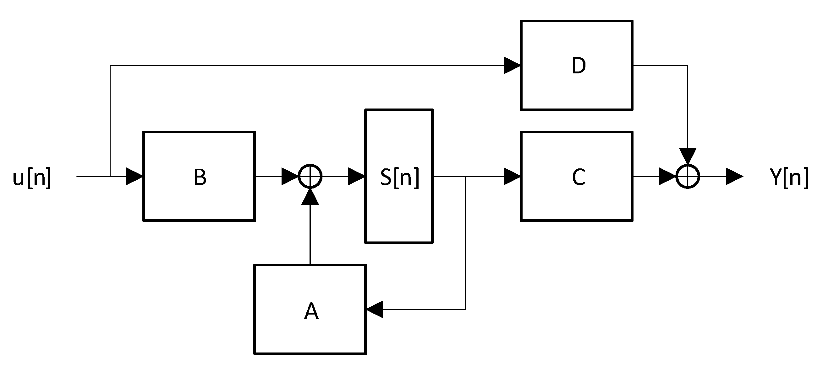
To introduce the equivalent ABCD model, let us consider the the vector $S\left[n\right]$ containing the information on the flip-flop states, shown in Equation (5).

$$S\left[n\right]={\left(d_0\left[n\right]d_1\left[n\right]d_{n-1}\left[n\right]\right)}^T,$$

(5)

where $d_i\left[n\right]$ indicates the state of the flip-flop i. Since the RSC encoder is composed by N flip-flops, $S\left[n\right]$ can encode $2^N$ possible combinations of states. In the same way, it is possible to use a vector $Y\left[n\right]$ to describe the encoded outputs $c_0\left[n\right]$ and $c_1\left[n\right]$, as illustrated in (6).

$$Y\left[n\right]={\left(c_0\left[n\right]c_1\left[n\right]\right)}^T.$$

(6)

For RSC encoders with a different value of R, since $Y\left[n\right]$ contains all the system outputs, $Y\left[n\right]$ is $N_o$ dimensional vector.

To describe the timing evolution of the RSC states and outputs with modulo-2 operations, we can exploit the ABCD model considering the current input and state:

$$\left\{\begin{array}{c}S[n+1]=A·S\left[n\right]+B·u\left[n\right]\\ Y\left[n\right]=C·S\left[n\right]+D·u\left[n\right]\end{array}\right.,$$

(7)

where $A,B,C,D$ are matrices, $u\left[n\right]$ is the input bit and $S[n+1]$ is the state at instant $n+1$.

A is $N\times N$ matrix; as it is shown in (7), A is function only of the linear feedback shift register (LFSR) structure, and it is made by the tap elements of $g\left(x\right)$, with $g\left(0\right)$ excluded, in the first row and a partial identical sub-matrix accountable of the shift operation in the second one.

$$A=\left(\begin{array}{ccccc}{g}_1& g_2& g_3& \cdots & g_N\\ & I_{(N-1)\times (N-1)}& & |& 0\end{array}\right),$$

(8)

where $I_{(N-1)\times (N-1)}$ indicates the $(N-1)\times (N-1)$ identity matrix and $g_1\dots g_N$ are the coefficients of the polynomial $g\left(x\right)$.

The B vector describe the impact of the current input to the state evolution. In case of a base realization of RSC code, the B vector is equal to the N dimensional vector shown in (9).

$$B={\left(\begin{array}{ccccc}1& 0& 0& \dots & 0\end{array}\right)}^T.$$

(9)

C is a $N_o\times N$ matrix representing the relation between the current state and the output coded bit. For RSC encoders that have code rate $R=\frac{1}{2}$, only two rows are present. In particular, since $c_0$ is the systematic output, which is only function of the input u, the first row of C is filled with zeros. On the contrary, the second row is computed by the $c_1$ parity output equation described by (10).

$$c_1\left[n\right]=h_0·u\left[n\right]+\sum _{i=1}^N(h_0·g_i+h_i)S\left[n\right],$$

(10)

where $h_i$ and $g_i$ are coefficients of the polynomials $h\left(x\right)$ and $g\left(x\right)$.

For RSC encoders having $N_o>2$ outputs, the ${(k+1)}^{th}$ row of C is populated by using the coefficients of the $h_k\left(x\right)$ polynomial according to Equation (10).

Finally, D is $N_o$-dimensional vector describing the contribution of the inputs in the generation of the output code. By using the systematic code $c_0\left[n\right]=u\left[n\right]$ and Equation (10), it is possible to retrieve the D vector values. For a $R=\frac{1}{2}$, the D vector is shown in Equation (11):

$$D=\left(\begin{array}{c}1\\ h_0\end{array}\right).$$

(11)

Equations (5)–(10) permit us to redraw the RSC circuit as a finite state machine described by the ABCD matrices model, whose block diagram is shown in Figure 2. For each operation, the modulo-2 operation is performed.

2.2. RSC Encoders Parallelization Approach

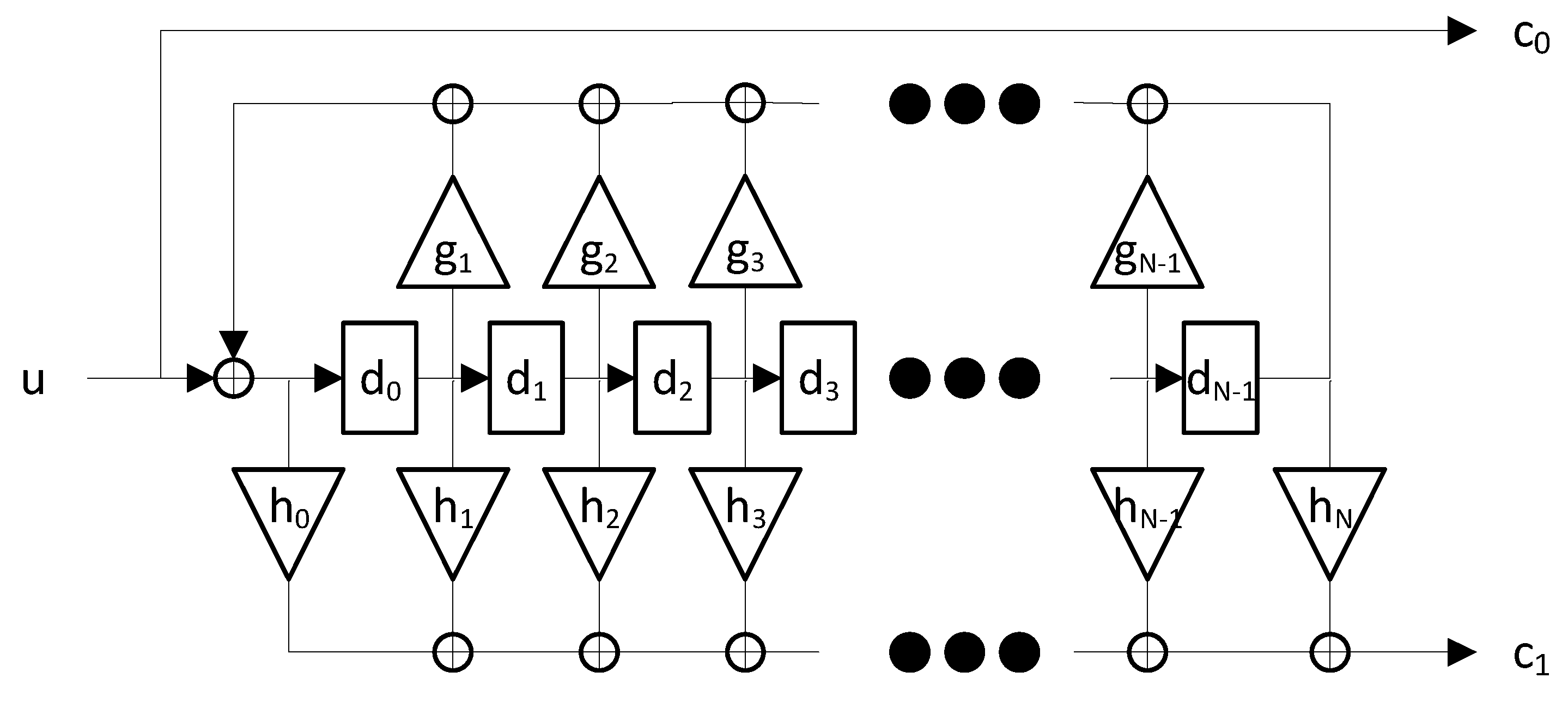
Increasing the parallelism of RSC encoders means to make it able to process k inputs at time. This means that in absence of puncturing, the vector the RSC encoder produces k vectors $Y\left[n\right]$ relative to the k inputs. In addition, it shall be considered that a k-dimensional input vector produces and update on the $S\left[n\right]$ of k steps at time. For such reason, a k parallel RSC encoder can be described by using an equivalent $A^{\prime }{B}^{\prime }{C}^{\prime }{D}^{\prime }$ model shown in Equation (12):

$$\left\{\begin{array}{c}S[n+k]=A^{\prime }·S\left[n\right]+B^{\prime }·\left(\begin{array}{c}u\left[n\right]\\ \cdots \\ u[n+k-1]\end{array}\right)\\ \left(\begin{array}{c}Y\left[n\right]\\ \cdots \\ Y[n+k-1]\end{array}\right)=C^{\prime }·S\left[n\right]+D^{\prime }·\left(\begin{array}{c}u\left[n\right]\\ \cdots \\ u[n+k-1]\end{array}\right)\end{array}\right.,$$

(12)

where $A^{\prime },B^{\prime },C^{\prime }$ and $D^{\prime }$ are the parallel matrices. In particular, the latter can be generated starting from the original A,B,C,D matrices by exploiting their proprieties and the information on the RSC encoder topology. For example, to calculate the $Y[n+k-1]$ output as a function of the $S\left[n\right]$ state and the k inputs $\left(u\right[n],\dots ,u[n+k-1\left]\right)$ it is sufficient to substitute the term $S[n+k-1]$ in the standard ABCD model equation (Equation (7)) for the state $S[n+k]$ with the same ABCD equation for the state $S[n+k-1]$, and to proceed recursively.

Equations (13)–(16) show the expressions of the matrices $A^{\prime }$,$B^{\prime }$,$C^{\prime }$ and $D^{\prime }$ as function of A,B,C,D.

$$A^{\prime }=A^k,$$

(13)

$$B^{\prime }=(A^{k-1}·B{A}^{k-2}·B\dots B),$$

(14)

$$C^{\prime }=\left(\begin{array}{c}C\\ \cdots \\ C{A}^{k-1}\end{array}\right),$$

(15)

$$D^{\prime }=\left(\begin{array}{ccccc}D& 0& 0& \cdots & 0\\ C·B& D& 0& \cdots & 0\\ & \ddots & & & \\ C·A^{k-1}·B& C·A^{k-2}·B& \cdots & C·B& D\end{array}\right).$$

(16)

In particular, $A^{\prime }$ shall be calculated by exploiting the A matrix properties. The latter can be derived directly from the LFSR theory and are described in Equations (17) and (18):

$$A^{2^N-1}=I_{N\times N}$$

(17)

$$A^k=A^{kmod(2^N-1)}$$

(18)

where $I_{N\times N}$ is the $N\times N$ identity matrix and the operator $mod$ indicates the module operation. Therefore, the sequence of $A^k$ matrices are a finite set of the $2^N-1$ matrices: $A^1$, $A^2$, $A^3$, …, $A^{2^N-2}$, $I_{N\times N}$.

Figure 3 shows the block diagram of a k-parallel RSC encoder.

In Section 2.1 we underlined that it possible to increase the code rate to improve the efficiency of the telecommunication system by puncturing the output code. In particular, it is important to underline that for a parallel RSC encoder particular puncturing schemes exist whose implementation do not require any additive logics; on the contrary, they also allow to reduce the complexity of the system. Indeed, let us express the puncturing scheme through a binary vector, whose null elements represent the punctured outputs. In this way, the implementation of puncturing schemes whose representative vector has a length equal to the number of rows of the $C^{\prime }$ and $D^{\prime }$ matrices is trivial. Indeed, to realize the puncturing, it is sufficient not to implement logics relative to rows of the $C^{\prime }$ and $D^{\prime }$ matrices having indexes equal to ones of the null elements in the puncturing scheme.

2.3. Parallel RSC Encoders Hardware Architecture

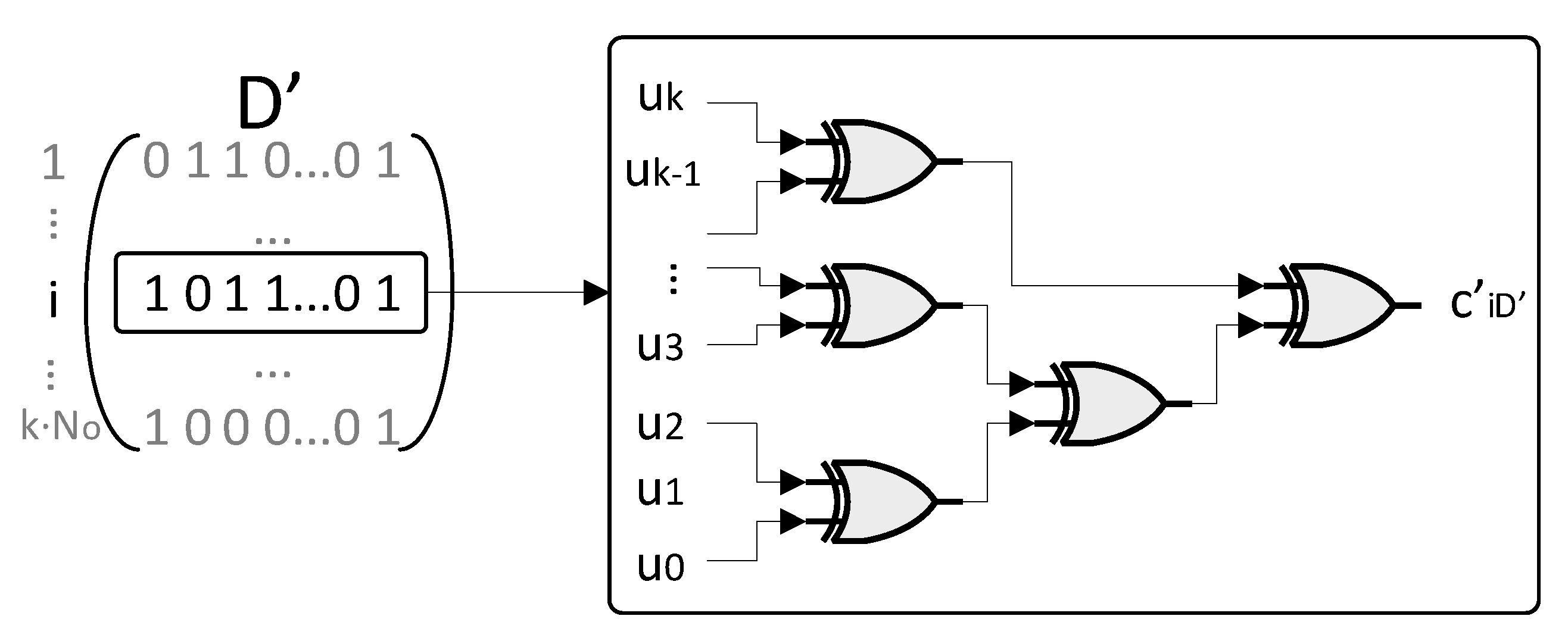
The parallel RSC encoder was implemented as VHDL intellectual property (IP) core. The architecture of the system matches the block diagram shown in Figure 3. The IP core can be exploit to generate a generic RSC encoder, which can be fixed by specifying $g\left(x\right)$, the puncturing scheme vector, and the matrix containing the feed-forward polynomials $h_k\left(x\right)$. Such vectors are necessary to generate the matrices $A^{\prime },B^{\prime },C^{\prime },D^{\prime }$. The information contained in these matrices is important to build the data path logics. Indeed, let us pose $Y=(c_0^{\prime }{c}_1^{\prime }\dots c_{k·N_o-1}^{\prime })$ and let us consider as example the generation of the output $c_i^{\prime }$. By isolating the contribution of the rows $D_i^{\prime }$ and $C_i^{\prime }$ of the matrix $C^{\prime }$ and $D^{\prime }$ in Equation (12), such output is calculated as shown in the system of Equation (19):

$$\left\{\begin{array}{cc}{c}_i^{\prime }\hfill & =c_{i{C}^{\prime }}^{\prime }+c_{i{D}^{\prime }}^{\prime }\hfill \\ c_{i{C}^{\prime }}^{\prime }\hfill & \triangleq C_i^{\prime }·S\left[n\right]\hfill \\ c_{i{D}^{\prime }}^{\prime }\hfill & \triangleq D_i^{\prime }·\left(\begin{array}{c}u\left[n\right]\\ \cdots \\ u[n+k-1]\end{array}\right)\hfill \end{array}\right.,$$

(19)

where $c_{i{C}^{\prime }}^{\prime }$ and $c_{i{D}^{\prime }}^{\prime }$ are respectively the contributions of the networks described by the rows $C_i^{\prime }$ and $D_i^{\prime }$.

In particular, $c_{i{D}^{\prime }}^{\prime }$ is produced by the network operating over the inputs of the RSC encoder; on the contrary, the term $c_{i{C}^{\prime }}^{\prime }$ is generated by the subsystem processing the internal flip-flop states. More specifically, only the inputs whose position corresponds to the ones of the unitary elements inside the $D_i^{\prime }$ row contribute to $c_{i{D}^{\prime }}^{\prime }$.

In view of that, for each element $c_{i{D}^{\prime }}^{\prime }$ a dedicated network is instantiated which sums through exclusive OR (XOR) operations the inputs specified by the unitary elements of the row $D_i^{\prime }$. In particular, the architecture of the network is designed to minimize the logical path from the inputs to the output. For such aim, the various XOR gates are linked in a tree fashion. In each layer of the tree, the elements of the previous layer are grouped into couples which feed a XOR gate. In case of an odd number of layer inputs, the last element is directly linked with the successive layer. When a matrix row $D_i^{\prime }$ is identically null, its contribution $c_{i{D}^{\prime }}^{\prime }$ is forced to 0, which is the neutral element for the XOR gate. This means that such row is not contributing to generate the output $c_i^{\prime }$.

Figure 4 shows the tree pattern of the network for the generation of $c_{i{D}^{\prime }}^{\prime }$.

The approach described for the generation of the output bits $c_i^{\prime }$ through the matrix rows $C_i^{\prime }$ and $D_i^{\prime }$ was also exploited to produce the inputs to the flip-flops through the rows $A_i^{\prime }$ and $B_i^{\prime }$. More specifically, the same network topology described for the matrix rows $D_i^{\prime }$ is also exploited for all the other matrices rows.

2.4. Analysis of the Tree Network Topology as a Function of the Parallelism Degree

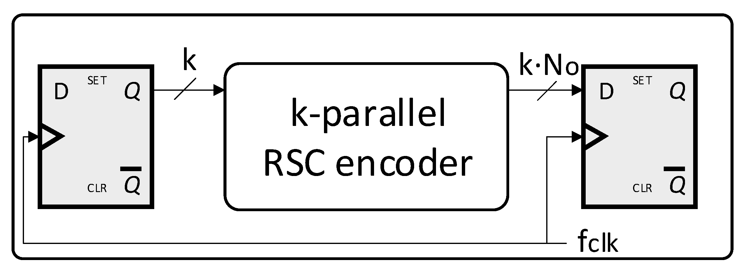
In Section 2.3 we described the VHDL IP core implementing a k parallel RSC encoder. In order to characterize the IP core, let us consider the scenario where the RSC encoder is stimulated by a source producing k input data synchronously with the rising or falling edge of clock signal with frequency $f_{clk}$. At the same time, let us suppose that the $k·N_o$ output code is sampled by a sink synchronously with the same reference clock signal. Such scenario is shown in Figure 5.

The method to increase the parallelism degree illustrated in Section 2.2 has the aim to increase the capacity of a RSC encoder to process the data produced by the source fast. In particular, one merit parameter is the system throughput. In view of that, it is possible to consider as merit parameter the input data rate $R_{IN}$. On the contrary, the output data rate is meaningless to characterize the processing speed of the system since it is dependent on the code rate R.

In the scenario shown in Figure 5, $R_{IN}$ can be calculated as described by Equation (20):

$$R_{IN}=k·f_{clk}.$$

(20)

Equation (20) shows that $R_{IN}\propto k$. Such relation might suggest that an increment of k leads to a proportional growth of $R_{IN}$. However, if we suppose to process data with the maximum clock frequency $f_{cl{k}_{MAX}}$ which guarantees the correct sampling of the output code to maximize $R_{IN}$, it shall be considered that $f_{cl{k}_{MAX}}$ depends on the critical path propagation delay $T_p$ according to the set-up time rule [22], which is shown in Equation (21):

$$f_{cl{k}_{MAX}}=\frac{1}{T_{sup}+T_p+T_{cq}},$$

(21)

where $T_{sup}$ is the set-up time of the sink register and $T_{cq}$ is the time necessary to the source register to stabilize the output data after the clock edge.

Although the network described by matrices $A^{\prime }$ and $C^{\prime }$ have constant number of inputs with the parallelism degree k, the dimension of the input vector for the networks described by matrices $B^{\prime }$ and $D^{\prime }$ is depending on k. It implies that the complexity of such networks grows with k; for such reason, it reasonable to assume that there is a dependency of $T_p$ on the parallelism degree. It leads to conclude that $f_{cl{k}_{MAX}}$ depends on k, making the relation $R_{IN}\left[k\right]$ not linear.

In order to derive such relation, it is possible to consider the tree network architecture described in Section 2.3. In particular, if we define $T_{p0}$ as the propagation delay of a single XOR gate, for such topology the total propagation delay can be estimated by using the expression shown in Equation (22).

$$T_p\left[k\right]\approx T_{p0}·\lceil log2\left({\mathsf{\Omega }}_{M^{\prime }i}\left[k\right]\right)\rceil ,$$

(22)

where ${\mathsf{\Omega }}_{M^{\prime }i}\left[k\right]$ indicates the number of unitary elements present in the row i of a generic matrix $M^{\prime }$. It is necessary to notice that Equation (22) does not take into consideration the delay due to the interconnections.

At the same manner, it is possible to study the dependency on the number of sources as function of the parallelism degree k.

Indeed, if we suppose that the first layer of the tree has ${\mathsf{\Omega }}_{M^{\prime }i}\left[k\right]$ unitary elements, $\lfloor \frac{{\mathsf{\Omega }}_{M^{\prime }i}\left[k\right]}{2}\rfloor$ XOR gates are necessary for the first layer. In the second layer, $\left(\begin{array}{c}\lfloor \frac{{\mathsf{\Omega }}_{M^{\prime }i}\left[k\right]}{4}\rfloor +(\lfloor \frac{{\mathsf{\Omega }}_{M^{\prime }i}\left[k\right]}{2}\rfloor mod2)\end{array}\right)$ XOR gates are necessary. For such reason, it is possible to consider the number of XOR gates composing a tree network roughly proportional to ${\mathsf{\Omega }}_{M^{\prime }i}\left[k\right]·\lceil log2\left({\mathsf{\Omega }}_{M^{\prime }i}\left[k\right]\right)\rceil$.

In particular, since for sufficiently high values of k the contribution of the $A^{\prime }$ and $C^{\prime }$ matrices is roughly constant, the number of XOR gates necessary to realization of the entire RSC encoder can be estimated through the Equation (23).

$$N_{XOR}\left[k\right]\approx N_0+N_1·{\mathsf{\Omega }}_{M^{\prime }i}\left[k\right]·\lceil log2\left({\mathsf{\Omega }}_{M^{\prime }i}\left[k\right]\right)\rceil ,$$

(23)

where $N_0$ and $N_1$ are constants to determine.

We shall also consider that in FPGA implementations the number of XOR does not match in general the number of slice LUTs used. For such reason, in such conditions the model described in Equation (23) represents a worse estimation of source utilization.

3. Results

3.1. BER Performance Analysis and Implementation Results of some RSC Codes

In our previous work [16], we showed the $BER=BER\left(\frac{E_b}{N_0}\right)$ curves of some RSC encoders with $R=\frac{1}{2}$, where $E_b$ is the average energy per bit, and $N_0$ is the power spectral density of a white Gaussian noise process. These curves were produced through a Matlab^® simulation including:

• RSC encoder
• Binary phase shift keying (BPSK) modulation
• Additive white Gaussian noise (AWGN) channel
• Soft-viterbi decoder

Such RSC encoders were synthesized on Zynq 7000 xc7z010clg400-1 FPGA by exploiting the architecture described in Section 2.3.

Table 1. Recursive systematic convolutional (RSC) encoders rate, occupation, code rate properties.

ID	L	Generators	Paral. (k)	Puncturing	Code Rate	${\mathit{f}}_{{\mathit{clk}}_{\mathit{MAX}}}$ (MHz)	${\mathit{R}}_{\mathit{IN}}$ (Mb/s)	Slice LUTs	Slice egs
RSC_1_1	3	$\left(\begin{array}{ccc}1& ;& \frac{1+x^2}{1+x+x^2}\end{array}\right)$	1	No	$\frac{1}{2}$	770.4	770.4	2	2
RSC_1_2	3	$\left(\begin{array}{ccc}1& ;& \frac{1+x^2}{1+x+x^2}\end{array}\right)$	2	[1 1 1 0]	$\frac{2}{3}$	640.6	1281.2	2	1
RSC_1_3	3	$\left(\begin{array}{ccc}1& ;& \frac{1+x^2}{1+x+x^2}\end{array}\right)$	3	[1 1 1 1 1 0]	$\frac{3}{5}$	648.9	1946.7	3	2
RSC_2_1	4	$\left(\begin{array}{ccc}1& ;& \frac{1+x+x^3}{1+x^2+x^3}\end{array}\right)$	1	No	$\frac{1}{2}$	784.9	784.9	2	2
RSC_2_2	4	$\left(\begin{array}{ccc}1& ;& \frac{1+x+x^3}{1+x^2+x^3}\end{array}\right)$	2	[1 1 1 0]	$\frac{2}{3}$	781.8	1563.7	3	3
RSC_2_3	4	$\left(\begin{array}{ccc}1& ;& \frac{1+x+x^3}{1+x^2+x^3}\end{array}\right)$	3	[1 1 1 1 1 0]	$\frac{3}{5}$	613.1	1839.3	4	3

shows the RSC codes chosen and their results in terms of number of maximum clock frequency, input data rate and FPGA sources. To estimate the maximum clock frequency, input and output registers were included as shown in Figure 5, and $f_{clk}=100MHz$ clock constraint was imposed. Such registers are not considered in the reported slice registers results of Table 1.

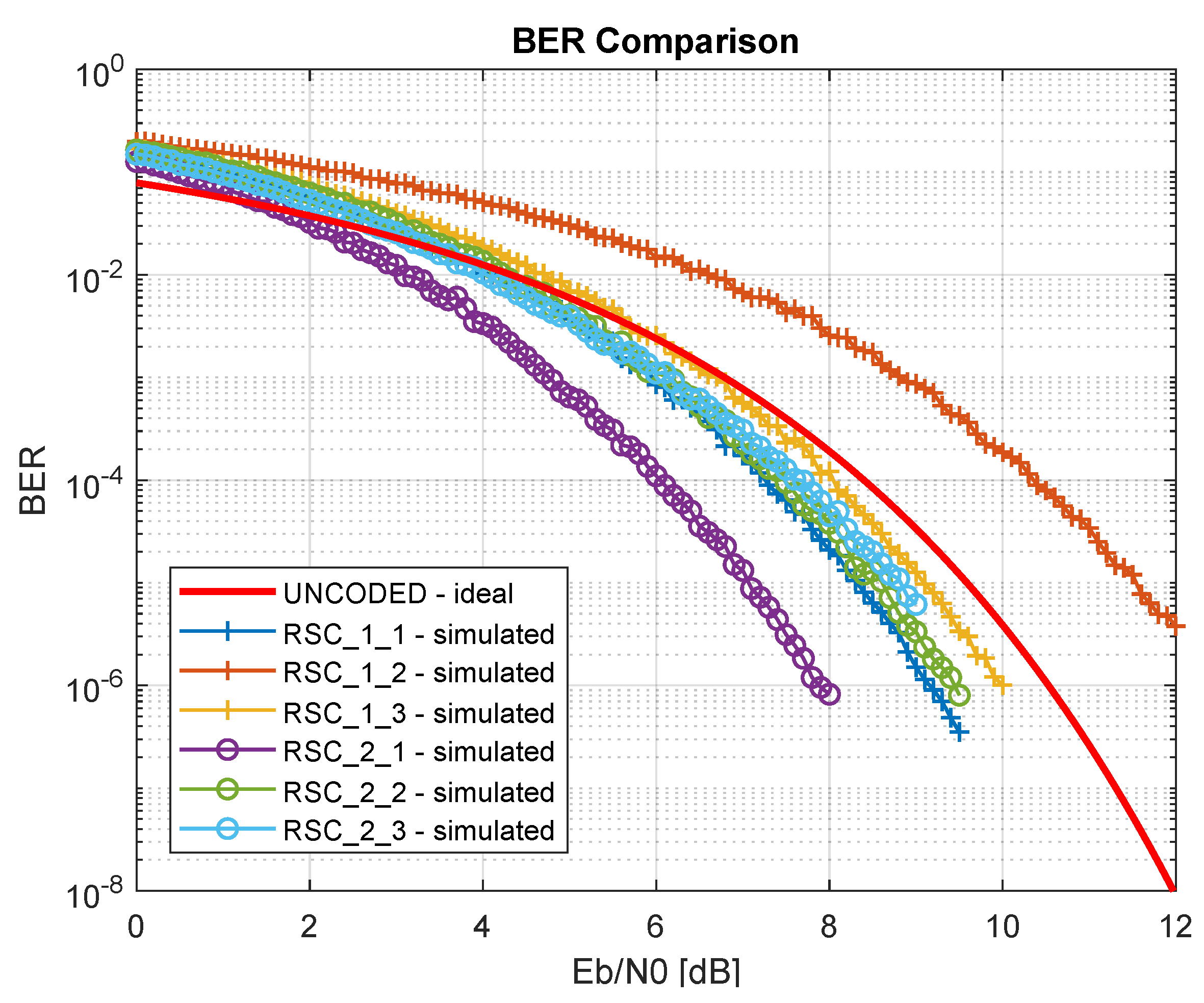
Figure 6 shows the BER curves resulting from the Matlab^® simulation.

Table 1 shows that an increment of the parallelism degree leads to augment of the input data rate $R_{IN}$, but it required a higher number of sources, especially slice LUTs.

Section 3.2 presents a deeper analysis of the $R_{IN}\left[k\right]$ trend through a case study.

3.2. Impact of the Parallelism Degree on the Data Rate: Case Study

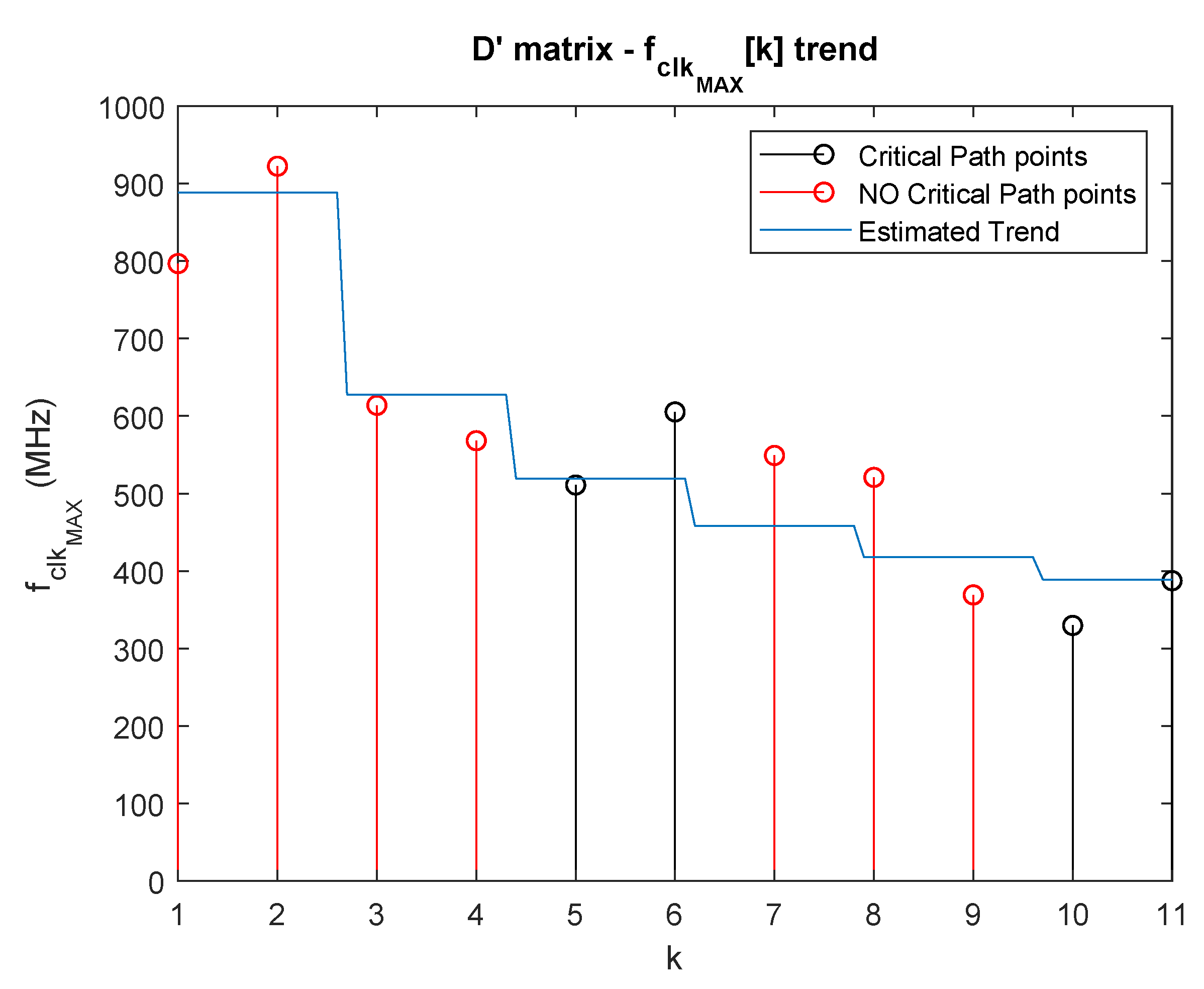
In this section, we present a case study that permits us to estimate the trend $R_{IN}\left[k\right]$ for the RSC encoder described by the generators shown in Equation (24) by applying the analysis reported in Section 2.4.

$$G\left(x\right)=\left(\begin{array}{ccc}1& ;& \frac{1+x+x^3}{1+x^2+x^3}\end{array}\right).$$

(24)

For such aim, it is necessary to estimate the dependency of the maximum clock frequency $f_{cl{k}_{MAX}}\left[k\right]$. The first difficulty is that the critical path might involve a different register—logics—register path for every different value of k. Even if this problem is real, in Section 2.4 we illustrate that for increasing values of k, only the networks relative to $B^{\prime }$ and $D^{\prime }$ matrices are increasing in complexity. In view of that, it is reasonable to deduce that for sufficiently high values of k the critical path is in one of the networks relatives to the rows of the matrices $B^{\prime }$ and $D^{\prime }$. Such hypothesis is confirmed by the FPGA implementation results shown in

Table 2. Results of the case study synthesis on Zynq 7000 xc7z010clg400-1 field programmable gate array (FPGA).

Parallel.	${\mathit{f}}_{{\mathit{clk}}_{\mathit{MAX}}}$	Matrix Containing	Parallel.	${\mathit{f}}_{{\mathit{clk}}_{\mathit{MAX}}}$	Matrix Containing
(k)	(MHz)	the Critical Path	(k)	(MHz)	the Critical Path
1	784.9293564	B	7	523.5602094	B
2	545.2562704	A	8	489.2367906	B
3	564.6527386	C	9	366.9724771	B
4	548.5463522	C	10	329.7065612	D
5	510.9862034	D	11	387.4467261	D
6	605.3268765	D

.

Table 2 shows that for $k\ge 5$ the critical path is included in the networks relative to $B^{\prime }$ and $D^{\prime }$ matrices.

Even if it is probable that for different values $k>11$ the critical path is not definitely included in the networks relative to a single matrix, it is necessary to consider that the both the $B^{\prime }$ and $D^{\prime }$ networks are implemented by using the same topology, whose propagation delay/parallelism grade trend can be described by Equation (22). For such reason, it is possible to approximate the function $f_{cl{k}_{MAX}}\left[k\right]$ by using $f_{cl{k}_{MA{X}_{M^{\prime }}}}\left[k\right]$. The latter describes the dependency of the maximum clock frequency as function of k of the paths relative to a generic matrix $M^{\prime }$. For such reason, $f_{cl{k}_{MAX}}\left[k\right]$ can be estimated by using the expression described by Equation (25):

$$f_{cl{k}_{MAX}}\left[k\right]\approx f_{cl{k}_{MA{X}_{M^{\prime }}}}\left[k\right]=\frac{1}{T_A+T_B·\lceil log2\left({\mathsf{\Omega }}_{M^{\prime }}\left[k\right]\right)\rceil },$$

(25)

where, $T_A$ and $T_B$ are parameters to determine, and where, similarly to Equation (22), the term ${\mathsf{\Omega }}_{M^{\prime }}\left[k\right]$ models the maximum number of unitary elements among the all networks relative to the matrix $M^{\prime }$ for a fixed value of k (note the absence of the subscript i), as described by Equation (26).

$${\mathsf{\Omega }}_{M^{\prime }}\left[k\right]=max\left\{{\mathsf{\Omega }}_{M^{\prime }i}\left[k\right]\right\}.$$

(26)

Parameters $T_A$ and $T_B$ of Equation (25) can be estimated by using data shown in Table 2 through a mean square error (MSE) interpolation. In particular, the trend $f_{cl{k}_{MAX}}\left[k\right]$ was approximated with trend of the networks relative to the matrix $D^{\prime }$. This is due to the fact the maximum number of unitary elements among the rows $D_i^{\prime }$ is always higher than the maximum number of unitary elements among the rows $B_i^{\prime }$ for each value of $k\in (1,\dots ,100)$. It was demonstrated through a Matlab^® simulation which calculated the maximum number of unitary elements for $B_i^{\prime }$ and $D_i^{\prime }$ depending on different values of k.

The same simulation was exploited to estimate the relation ${\mathsf{\Omega }}_{D^{\prime }}\left[k\right]$ for the matrix $D^{\prime }$. Such a trend is difficult to derive by simply exploiting Equations (11) and (16). Nevertheless, it possible to realize an estimator $\overline{{\mathsf{\Omega }}_{D^{\prime }}\left[k\right]}$ through a machine learning approach. First of all, the model described in Equation (27) was used:

$$\overline{{\mathsf{\Omega }}_{D^{\prime }}\left[k\right]}=\parallel {\theta }_0+{\theta }_1·k\parallel ,$$

(27)

where $\parallel ·\parallel$ indicates the rounding operation; ${\theta }_0$ and ${\theta }_1$ are the learning parameters.

The relation, previously calculated, reporting the maximum number of unitary elements respectively in the rows of and $D^{\prime }$ matrix for each value of k in the range $(1,\dots ,100)$ was used to realize a dataset. The latter was randomly partitioned into a train and a test datasets, whose dimensions are respectively $\frac{2}{3}$ and $\frac{1}{3}$ of the original one. The values of the learning parameters ${\theta }_0$, ${\theta }_1$ were estimated through a mean square error approach on the training set, without considering the rounding operation.

A total of 20 iterations were performed; during each iteration the random partition of the total dataset was changed and the accuracy of the estimator is calculated on the test dataset. In particular, accuracy was calculated as the percentage of right predictions on the test dataset.

At the end of the procedure, the learning parameters relative to the partition with maximum accuracy on the test dataset were considered.

The best accuracy on the test dataset was of $87.87\%$ and the obtained learning parameters are shown in

Table 3. Learning parameters for the $\overline{{\mathsf{\Omega }}_{D^{\prime }}\left[k\right]}$ estimator.

${\mathit{\theta }}_0$	0.988904449419594
${\theta }_1$	0.571261448964218

.

$\overline{{\mathsf{\Omega }}_{D^{\prime }}\left[k\right]}$ was used for the estimation of the parameters $T_A$ and $T_B$. To increase the number of data to use for the interpolation process, we also exploited the values of the maximum clock frequency for the networks relative to the matrix $D^{\prime }$ for such values of k for which the system critical path was included in the network describing the rows of another matrix.

Table 4. $T_A$ and $T_B$ values derived through a mean square error (MSE) interpolation.

${\mathit{T}}_{\mathit{A}}$ [s]	3.25590031598599e-10
$T_B$ [s]	7.99924552672264e-10

reports the $T_A$ and $T_B$ values derived through the described methodology.

Figure 7 shows the estimated $f_{cl{k}_{MAX}}\left[n\right]$ trend and data used for the interpolation.

Equation (28) sums up the expression for the $R_{IN}\left[k\right]$ trend.

$$R_{IN}\left[k\right]=k·f_{cl{k}_{MAX}}\left[k\right]=\frac{k}{T_A+T_B·\lceil log2(\parallel {\theta }_0+{\theta }_1·k\parallel )\rceil }.$$

(28)

3.3. Impact of the Parallelism Degree on the Source Utilization: Case Study

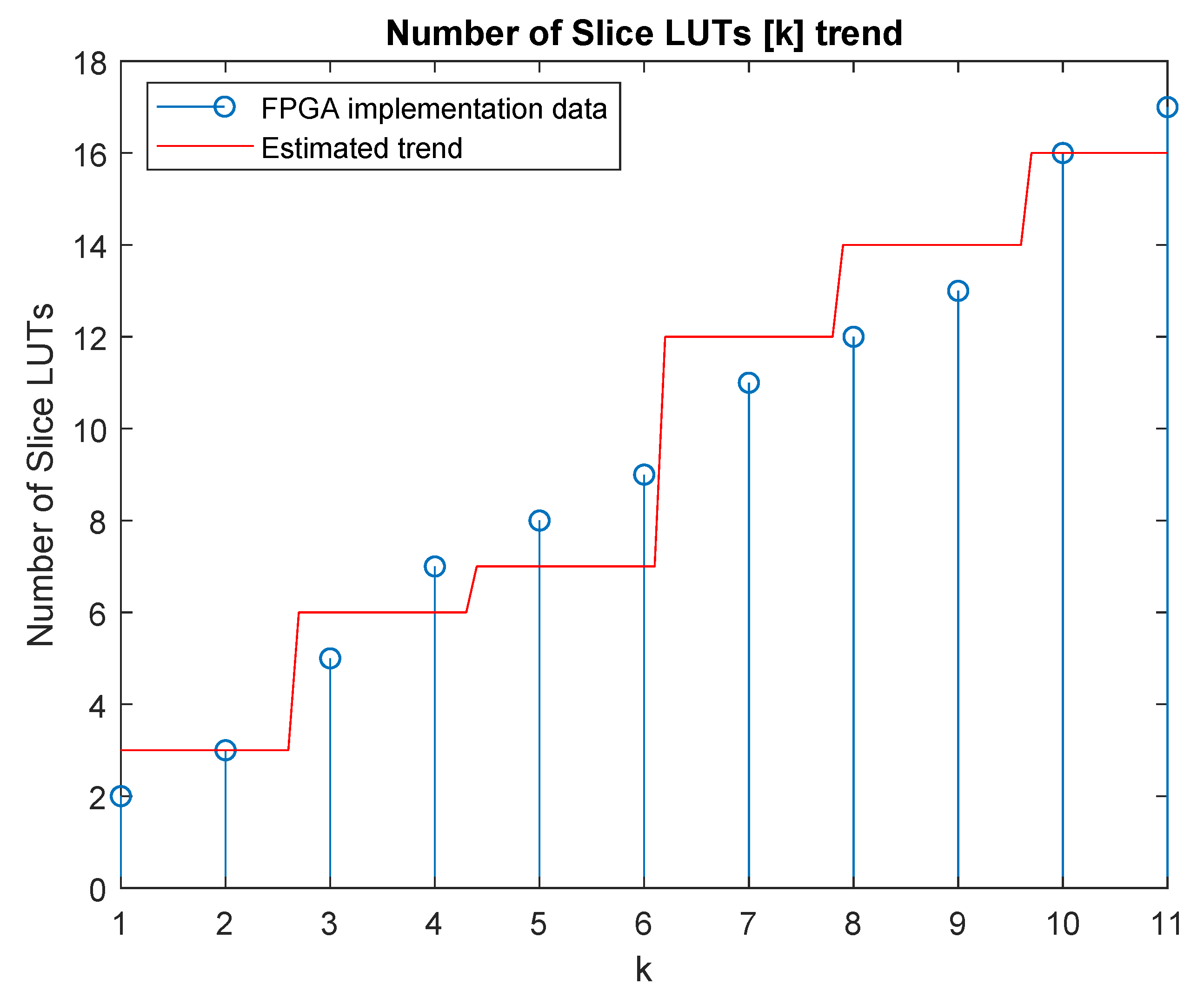
In this section, we describe a methodology to estimate the dependency of the number of slice LUTs depending on the parallelism degree by considering as case study the RSC encoder shown in Equation (24).

By using a similar approach to the one described in Section 3.2, $N_0$ and $N_1$ parameters of Equation (23) were estimated by using a MSE approach. In particular, ${\mathsf{\Omega }}_{D^{\prime }}\left[k\right]$ was measured by using the estimator described in Equation (27) and by exploiting the values of the learning parameters described in Table 3. The interpolation was performed by using data on slice LUTs utilization obtained by the multiple implementation of the RSC encoder on board Zynq 7000 xc7z010clg400-1 FPGA; such data are shown in

Table 5. Number of Zynq 7000 xc7z010clg400-1 FPGA-slice lookup tables (LUTs) for different k values.

Parallel.	Number of	Parallel.	Number of
(k)	Slice LUTs	(k)	Slice LUTs
1	2	7	11
2	3	8	12
3	5	9	13
4	6	10	16
5	8	11	17
6	9

.

Table 6. $N_0$ and $N_1$ values derived through a MSE interpolation.

${\mathit{N}}_0$	1.91672252010724
$N_1$	0.655328418230563

shows the $N_0$ and $N_1$ values found.

Owing to the real nature of the $N_0$ and $N_1$ parameters, the result was rounded to obtained an integer estimation. Figure 8 shows the estimated dependency of the number of slice LUTs on the parallelism degree.

4. Discussion

Data presented in Section 3.1 complete the results shown in our previous work [16], by providing information about the implementations of the various RSC encoders on FPGA. This provides an additional characterization of such encoders in terms of their speed performances and their source occupation.

The most important contribution of this work is linked to the analysis performed in Section 3.2 and Section 3.3 which permitted to extrapolate the dependency of the input data rate and the FPGA slice LUTs on the parallelism degree.

Such analysis, even if approximated, provides a description complete of the most important merit parameters of the implementation, allowing to choose the values of k depending on the different application requirements.

In particular, it is useful to notice that an increment of k leads to a less than proportional improvement of the $R_{IN}\left[k\right]$ value but requires a more than proportional increment of the number of used sources.

In addition, even if this analysis is performed for a specific RSC encoder, the methodology applied and the results is general are valid. In fact, the trends estimated do not depend on the polynomials $h_k\left(x\right)$ and $g\left(x\right)$ but only on the topology of the network used.

The validity of such results might be compromised by modifications of the topology of the network, e.g., an insertion of pipeline registers would lead to a different $R_{IN}\left[k\right]$ trend. Nevertheless, such optimization is linked to the single implementation and of difficult generalization.

5. Conclusions

This article presents a hardware IP core for the implementation of parallel RSC encoders. The architecture is based on the $A^{\prime }{B}^{\prime }{C}^{\prime }{D}^{\prime }$ model of a RSC encoder, which can be obtained through the methodology presented in our previous work [16]. The IP cores associate to each matrix an equivalent hardware network, based on a tree pattern for the minimization of the logics path.

Through a case study and an analysis of the proposed topology, the article provides an estimation of the trends of the input data rate and slice LUTs occupation depending on the parallelism degree which, together with the BER curves, provides a complete description of the merit parameters which are relevant for such devices.

References

- CCSDS. Flexible Advanced Coding And Modulation Scheme For High Rate Telemetry Applications; Recommendation for Space Data System Standards, CCSDS 131.2-B-1; CCSDS: Washington, DC, USA, 2012. [Google Scholar]
- Douillard, C.; Jézéquel, M.; Berrou, C.; Brengarth, N.; Tousch, J.; Pham, N. The turbo code standard for DVB-RCS. In Proceedings of the 2nd International Symposium on Turbo Codes Related Topics, Brest, France, 4–7 September 2000; pp. 535–538. [Google Scholar]
- Park, S.J.; Jeon, J.H. Interleaver optimization of convolutional turbo code for 802.16 systems. IEEE Commun. Lett. 2009, 13, 339–341. [Google Scholar] [CrossRef]
- Viterbi, A. Error bounds for convolutional codes and an asymptotically optimum decoding algorithm. IEEE Trans. Inf. Theory 1967, 13, 260–269. [Google Scholar] [CrossRef]
- Bahl, L.; Cocke, J.; Jelinek, F.; Raviv, J. Optimal decoding of linear codes for minimizing symbol error rate (corresp.). IEEE Trans. Inf. Theory 1974, 20, 284–287. [Google Scholar] [CrossRef]
- Benedetto, S.; Montorsi, G. Role of recursive convolutional codes in turbo codes. Electron. Lett. 1995, 31, 858–859. [Google Scholar] [CrossRef]
- Berrou, C.; Glavieux, A.; Thitimajshima, P. Near Shannon limit error-correcting coding and decoding: Turbo-codes. In Proceedings of the ICC’93-IEEE International Conference on Communications, Geneva, Switzerland, 23–26 May 1993; pp. 1064–1070. [Google Scholar]
- Benedetto, S.; Divsalar, D.; Montorsi, G.; Pollara, F. Serial concatenation of interleaved codes: Performance analysis, design, and iterative decoding. IEEE Trans. Inf. Theory 1998, 44, 909–926. [Google Scholar] [CrossRef]
- Berrou, C.; Pyndiah, R.; Adde, P.; Douillard, C.; Le Bidan, R. An overview of turbo codes and their applications. In Proceedings of the European Conference on Wireless Technology, Paris, France, 3–5 October 2005; pp. 1–9. [Google Scholar]
- Shannon, C.E. Communication in the presence of noise. Proc. IEEE 1998, 86, 447–457. [Google Scholar] [CrossRef]
- Weithoffer, S.; Nour, C.A.; Wehn, N.; Douillard, C.; Berrou, C. 25 Years of Turbo Codes: From Mb/s to beyond 100 Gb/s. In Proceedings of the 2018 IEEE 10th International Symposium on Turbo Codes Iterative Information Processing (ISTC), Hong Kong, China, 3–7 December 2018; pp. 1–6. [Google Scholar]
- Ilango, P.; Chokkalingam, A. A Novel Architecture of Modified Turbo Codes with an area efficient high speed interleaver. Concurr. Comput. Pract. Exp. 2018, e5067. [Google Scholar] [CrossRef]
- Fowdur, T.P.; Beeharry, Y.; Soyjaudah, S.K. Performance of modified asymmetric LTE Turbo codes with reliability-based hybrid ARQ. In Proceedings of the 2014 9th International Symposium on Communication Systems, Networks Digital Sign (CSNDSP), Manchester, UK, 23–25 July 2014; pp. 928–933. [Google Scholar]
- Kumar, M.S.; Shameem, S.S.; Raghu Sai, M.N.V.; Nikhil, D.; Kartheek, P.; Kishore, K.H. Efficient and low latency turbo encoder design using Verilog-Hdl. Int. J. Eng. Technol. 2018, 7, 37–41. [Google Scholar] [CrossRef]
- Jiang, S.; Zhang, P.W.; Lau, F.C.M.; Sham, C.W.; Huang, K. A Turbo-Hadamard Encoder/Decoder System with Hundreds of Mbps Throughput. In Proceedings of the 2018 IEEE 10th International Symposium on Turbo Codes Iterative Information Processing (ISTC), Hong Kong, China, 3–7 December 2018; pp. 1–5. [Google Scholar]
- Pilato, L.; Meoni, G.; Fanucci, L. Design Optimization for High Throughput Recursive Systematic Convolutional Encoders. In Proceedings of the 2018 22nd International Conference on System Theory, Control and Computing (ICSTCC), Sinaia, Romania, 10–12 October 2018; pp. 806–809. [Google Scholar]
- Singh, B.; Singh, I.P. Performance enhancement of LOG MAP Turbo Decoder for mobile applications. In Proceedings of the 2015 International Conference on Recent Developments in Control, Automation and Power Engineering (RDCAPE), Noida, India, 12–13 March 2015; pp. 259–264. [Google Scholar]
- Thul, M.J.; Wehn, N. FPGA implementation of parallel turbo-decoders. In Proceedings of the SBCCI 2004, 17th Symposium on Integrated Circuits and Systems Design (IEEE Cat. No. 04TH8784), Pernambuco, Brazil, 7–11 September 2004; pp. 198–203. [Google Scholar]
- Zynq7000 Datasheet. Available online: https://www.xilinx.com/support/documentation/data_sheets/ds190-Zynq-7000-Overview (accessed on 23 April 2019).
- Dhaliwal, S.; Singh, N.; Kaur, G. Performance analysis of convolutional code over different code rates and constraint length in wireless communication. In Proceedings of the 2017 International Conference on I-SMAC (IoT in Social, Mobile, Analytics and Cloud) (I-SMAC), Palladam, India, 10–11 February 2017; pp. 464–468. [Google Scholar]
- Bolinth, E. On the equivalence of rate R= k/n non-systematic feed-forward convolutional codes and recursive systematic convolutional codes. In Proceedings of the 11th European Wireless Conference 2005-Next Generation wireless and Mobile Communications and Services, Nicosia, Cyprus, 10–13 April 2005; pp. 1–7. [Google Scholar]
- Rabaey, J.M.; Chandrakasan, A.P.; Nikolic, B. Digital Integrated Circuits; Prentice-Hall: Upper Saddle River, NJ, USA, 2002; Volume 2. [Google Scholar]
Figure 1.
Architecture of a recursive systematic convolutional (RSC) encoder with .
Figure 2.
Block diagram of the ABCD matrices model of an RSC encoder.
Figure 3.
Block diagram of a k-parallel RSC encoder.
Figure 4.
Tree fashion network implementing the logics described in the row .
Figure 5.
RSC encoder in a scenario with synchronous source and sink registers.
Figure 6.
RSC encoders bit error rate curves.
Figure 7.
Estimated trend relative to the matrix.
Figure 8.
Estimated trend of the number of lookup tables (LUTs) as function of k.