Comparison of the Results of a Data Envelopment Analysis Model and Logit Model in Assessing Business Financial Health †

Department of Accounting and Controlling, Faculty of Management, University of Prešov, Konštantínova 16, 080 01 Prešov, Slovakia
*
Author to whom correspondence should be addressed.
†
This paper is an extended version of our paper published in the 27th Interdisciplinary Information Management Talks, 4–6 September 2019, Kutná Hora, Czech Republic.
Information 2020, 11(3), 160; https://doi.org/10.3390/info11030160
Submission received: 31 January 2020
/
Revised: 9 March 2020
/
Accepted: 11 March 2020
/
Published: 17 March 2020
(This article belongs to the Special Issue Digital Transformation in Economy, Business, Society and Technology)
Abstract
:This paper focuses on business financial health evaluation with the use of selected mathematical and statistical methods. The issue of financial health assessment and prediction of business failure is a widely discussed topic across various industries in Slovakia and abroad. The aim of this paper was to formulate a data envelopment analysis (DEA) model and to verify the estimation accuracy of this model in comparison with the logit model. The research was carried out on a sample of companies operating in the field of heat supply in Slovakia. For this sample of businesses, we selected appropriate financial indicators as determinants of bankruptcy. The indicators were selected using related empirical studies, a univariate logit model, and a correlation matrix. In this paper, we applied two main models: the BCC DEA model, processed in DEAFrontier software; and the logit model, processed in Statistica software. We compared the estimation accuracy of the constructed models using error type I and error type II. The main conclusion of the paper is that the DEA method is a suitable alternative in assessing the financial health of businesses from the analyzed sample. In contrast to the logit model, the results of this method are independent of any assumptions.
1. Introduction
Diagnosing the financial health of a company, as well as predicting its failure, is currently a highly discussed topic. In order to maintain prosperity and competitiveness, it is extremely important for a company to know the financial situation that it is in. Adequate management decisions cannot be made without detailed analyses of business financial health. An important prerequisite for effective decision-making of business owners is a high-quality, comprehensive, and timely diagnosis, supported by a detailed analysis of adverse phenomena threatening the company’s operations. Based on these results, management of the company can take effective measures to improve the financial situation. The results of the analyses are of great importance, not only for business owners and managers, but also for investors and banks, as they largely determine all their decisions in relation to businesses. A company that fulfils two basic conditions is considered to be a financially sound and liquid enterprise—it is able to repay its liabilities in time, while at the same time it is profitable, thus achieving a return on invested capital. If an enterprise does not meet these two conditions, it is in financial distress that may end in bankruptcy. In defining the problems that accompany financial distress, some authors tend to focus on negative operating revenues and problems with cash flow [1,2,3]. Some other authors focus on problems with the decline in profits [4,5,6,7]. In general, the term financial distress has as a negative connotation regarding the financial health of an enterprise that is suffering from a lack of liquidity and inability to pay its liabilities [8]. At present, there are two major trends in the area of financial distress prediction. The first trend is aimed at describing a situation in which a company is failing financially by detecting the symptoms of failure [9,10,11,12]. The second trend is to compare the estimation accuracy of individual prediction models [13,14]. Bankruptcy prediction models are used to detect early signals of significant bankruptcy risks and to identify companies facing potential bankruptcy [15]. The purpose of these models is to help businesses find out whether they are in danger of bankruptcy in the near future. They have been drawn up on the basis of the results of scientific research and are mostly intended for a specific group of enterprises according to their field of activity. The essence of these models is that businesses were experiencing anomalies for some time before bankruptcy, and the values of the indicators of prosperous enterprises differ significantly from those of non-prosperous enterprises. Prediction models can give the company a certain degree of probability of the occurrence of negative situation. Based on the above, our study focuses on the estimation accuracy of selected models.
In this paper, we aimed to assess financial health and predict failure of businesses from the Slovak heat industry by applying the data envelopment analysis (DEA) model. With the use of this model, we identified businesses on the financial health frontier. Moreover, for businesses that do not lie on this frontier, we calculated goal values of inputs and outputs to become financially healthy and efficient, respectively. On the other hand, we also identified businesses threatened with bankruptcy that lie on the financial distress frontier. We also aimed to verify the results of the DEA model with the use of a logit model. For this purpose, we determined the estimation accuracy of selected models.
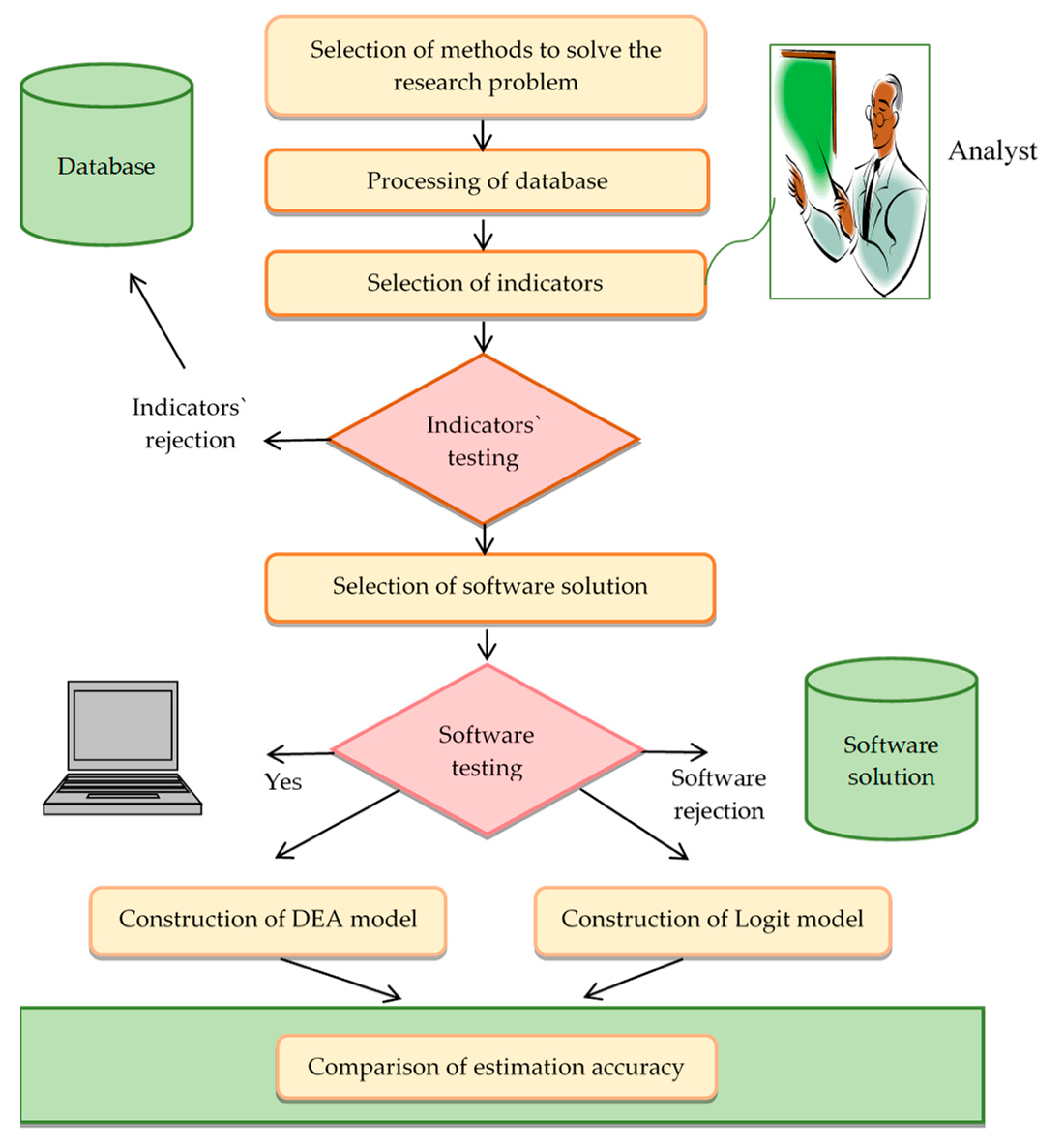
The remainder of the paper is structured as follows. At the end of Section 1, the research problem and the aim of the paper are formulated. Section 2 is the literature review. This section lists various methods and models designed to assess business financial health and to detect its failure. A special part of Section 2 is devoted to the overview of the theoretical knowledge about the DEA method. Section 3 describes the research sample, selection of indicators, and theoretical background of applied models. The main models used in the paper are the BCC DEA model processed in DEAFrontier software and the logit model constructed in Statistica software. Section 4 lists the results for the BCC DEA model, which were verified by applying the logit model. Section 5 includes the discussion, in which the results achieved in this paper are compared with the results of other studies. This section also summarizes the essential conclusions resulting from the research and presents the significant findings. The process of the research is illustrated in Figure 1.
We set the following research question: Is the DEA method a suitable alternative in assessing the financial health of businesses from the analyzed sample?
In accordance with the research problem, we set the following aim of the paper—to verify the results of the DEA model with the result of the logit model.
2. Literature Review
Nowadays, there are many models, both theoretical and practical, designed to detect problems and predict business bankruptcy. Many of these models are based on mathematical and statistical methods (mainly regression models and discriminant analysis). Bankruptcy prediction models can be divided into three groups [8,16]: statistical models, models using artificial intelligence, and theoretical models. Statistical models can be classified into two groups: univariate and multivariate models. Multivariate statistical models include multiple discriminant analysis models, linear probability, logit models, probit models, and the total cumulative and partial adjustment processes [17]. In [18], the authors specifically point to three trends: the transition from univariate analysis of variables to multivariate prediction, a shift from classical statistical methods to machine learning methods based on artificial intelligence, and more intensive involvement of hybrid and ensemble classifiers [19].
General progress in technology development has resulted in the emergence of new models, including logit and probit analyses and neural networks. At present, however, the trend is to only modify the already existing models, which is also confirmed by the fact that no new methodology has been proposed in recent decades. The prediction accuracies of different models seem to be generally comparable, although artificially intelligent expert system models perform marginally better than statistical and theoretical models. Individually, the use of multiple discriminant analysis (MDA) and logit models dominates the research [16].
The study by [20] was the first to demonstrate that financial ratios can be useful in the prediction of an individual firm’s failure. He compiled an extensive database from which he used thirty ratios to predict future development. The average value of these indicators was compared with the indicators of companies which later went bankrupt. Beaver pointed out that financial indicators may be useful in predicting the failure of individual firms [21]. He has also proved that not all financial indicators can be used for this prediction. This has also been confirmed in practice, where the use of simple financial indicators have been questioned because of their possible distortion by management decisions. Therefore, Beaver suggested using a dichotomous classification test [22]. Using this method, multiple financial indicators with the greatest prediction accuracy are identified. These indicators are used as one predictor with several degrees of freedom. The essence of this method is to find a linear combination of characteristics that best distinguishes two groups of businesses, namely those that are threatened with bankruptcy and non-bankrupt businesses [23]. Univariate analysis was later followed by multivariate discriminant analysis. In 1968, Altman developed a multiple discriminant analysis model (MDA) known as the Z-score. Since Altman’s study [24], the number and complexity of these models has increased significantly. As already mentioned, in the early period of the prediction models, discrimination analysis was very popular. This method was applied by [20,24,25,26,27,28,29,30,31]. Altman’s original model required the fulfilment of multinormality, homoskedasticity, and linearity assumptions. These assumptions were often not met for financial indicators. In the event that any of the variables were categorical, this method gave distorted results [32]. The main drawback of this method, however, was that although it is able to identify businesses that are threatened with bankruptcy, it is not able to estimate the likelihood of this situation occurring. In the conditions of Slovakia and the Czech Republic, models were formulated that corresponded to the requirements placed on these models. In 1999, Binkert formulated the MDA model, also called the Binkert model. His sample consisted of 160 enterprises (80 bankruptcies). It is necessary to mention the model of Chrastinová, called the Ch index (1998), which was processed for agricultural enterprises (1123 enterprises), as well as Gurčík’s model (2003), the G index, which was designed to predict the financial condition of agricultural enterprises (60 enterprises). Of the Czech authors, we can mention Neumaierová and Neumaier and their models, namely the IN95 creditor model, the IN99 proprietary model (1968 enterprises), the IN01 combined proprietary–creditor model (1915 enterprises), and the IN05 model (1526 enterprises). In 2008, Růčková formulated the MDA model, also known as the so-called Růčková model. In the area of banking, Gurný and Gurný (GaG) formulated model I in 2009 and model II in 2009 [8].
Taking into account the shortcomings of methods based on discrimination analysis, the next step in the theory of bankruptcy prediction was to develop methods and models that would be able to provide information about the probability of business bankruptcy [33]. This was the reason why logistic regression began to be preferred. This method is used mainly for models that have a dichotomous output variable [34]. Compared to methods based on multidimensional discrimination analysis, logistic regression has several advantages. Compared to discrimination analysis, it has a higher predictive ability and its application does not require compliance with assumptions that could limit its usability. The main advantages of logistic regression include unnecessary normal distribution of independent variables, unnecessary testing of the importance of individual variables prior to the analysis, as well as non-equality of variance–covariance matrices [35]. This method was first used to predict the bankruptcy of banks by [36]. The first study to use it in companies was [37]. As a pioneer in the application of logit analysis, one author disagreed with the application of discrimination analysis to predict bankruptcy due to the requirement for the same variance–covariance matrix [38]. The logit model provides the ability to model complex relationships between variables, however at the same time assumes a log–linear relationship between the response variables and the explanatory variables. Logistic regression is particularly useful when predicting binary outputs based on continuous independent variables. It should be noted that discrimination analysis may be more useful for small data, however logistic regression is more appropriate for larger samples [39]. However, even logit models have their weakness, which is the sensitivity to remote observation.
The probit model is used less often because it is more complicated to calculate [40]. The first person who used the probit model was [41]. The main difference between logit and probit models is in their definition of the function f (*). While the logit model uses the cumulative distribution function of the logistic regression, the probit model uses the cumulative distribution function of the standard normal distribution. The conclusions of both methods are similar but not identical. While the logit model is preferred in health sciences, the probit model is preferred by economists and political scientists. The probit model takes into account the non-standard deviations of errors in more advanced econometric settings [42]. The advantage of the logit and probit analyses is that their outputs lie between 1 and 0, and directly indicate the probability of a business failure. The big advantage is that it is possible to use an artificial variable to express an independent qualitative variable, the value of which is not continuous but belongs to one of the given categories [3]. In 2014, Altman presented a new prediction model based on the application of discriminant analysis and 7 modifications of the logit model. It was confirmed that these models are applicable in Slovakia [43]. However, it should be pointed out that it is not possible to easily apply models in other countries and different industries. From the logit models formulated in the Czech Republic, we can mention Jakubík–Teplý model [44]. Its authors applied the data for 757 businesses and achieved an 80.41% success rate. In 2012, [45] formulated logit model I and logit model II. The logit model proposed by Hurtošová was established in the Slovak Republic in 2009. Newer logit models include the Gulka model in 2016, the model proposed by Harumová and Janisová in 2012, and Delina and Packová’s model from 2013 [8].
The last group of methods we deal with in our paper contains mathematical programming methods. Within the framework of mathematical programming, there is a problem of linear programming, where the challenge is to find the extreme value of a function. This is a task where the objective function is linear and the set for which we are looking for extreme values is a system of linear equations [8]. The goal of the linear programming is to find the optimal value, so that all ratios are based on the optimal solution. This model creates preconditions for economic analyses. In designing the model, particular attention should be paid to the accuracy of the determination of individual constraints. The practical solution of a given task should be based on its simplified version. The most widespread algorithm for solving linear programming tasks is the simplex method. The authors of [46] or [47] were the first to apply linear programming to predict financial health. One of the methods based on mathematical programming is the DEA method [48]. Compared to statistical methods, DEA is a relatively new, non-parametric method, which represents one of the possible approaches to assessing the financial health of a businesses and its risk of bankruptcy [49]. This method was first applied in 1978 by [50]. It is based on the idea mentioned in the article “Measuring the Efficiency of Decision Making Units“, published by [51] in 1957. His work was based on the works of [52] and [53]. In this, [51] proposed a new approach to efficiency measuring based on a convex efficient frontier and the use of distance measurement functions between the enterprise of interest and the projected point on the efficiency frontier. In this way, he proposed a new level of efficiency based on the calculation of two components of the overall business efficiency: technical efficiency and resource allocation efficiency. Farrel’s approach is based on measuring the ability of business to transform inputs into outputs and is, therefore, also called an input-oriented approach. Another study [50] applied a multiplicative input–output model to measure business efficiency. The approach of these authors represents a two-step efficiency calculation. The first step is to identify the efficiency frontier, whereby businesses positioned at this frontier are among the best businesses. The second step is to calculate the efficiency scores for the analyzed businesses and their distances from the efficiency frontier. DEA models can be divided into DEA CCR [50] and DEA BCC [54] in terms of whether each input unit produces the same amount of outputs or variable amounts of outputs. This method was further developed by [55]. The DEA method was also used by [56,57,58,59,60,61,62,63,64,65,66,67] and many others. The DEA model is often applied in calculating the efficiency of medical facilities [68,69,70,71].
The DEA method was first used to predict bankruptcy by [72], who first compared its results with the results of Altman’s Z-score. At the time when this model was applied, DEA models had not yet been applied in the context of bankruptcy prediction. This research has proven to have various application possibilities. Other authors dealing with the DEA bankruptcy prediction included [73], who used the DEA radial model to predict bankruptcy and compared its results with discriminant analysis (DA) results. In the same year, [74] applied an additive and radial model with the use of the peeling technique. This model achieved 100% success in predicting business bankruptcy. In 2009, [75] used an additive DEA model and compared its results with the results of logistic regression. The result of this study was a satisfactory rate of correct prediction of business bankruptcy; less accurate was the prediction rate for financially healthy businesses. In 2009, [76] applied an additive DEA model to create a financial distress frontier. The results were then compared with the DEA–DA approach. In 2011, [77] combined the radial and additive DEA model and created the DEA ranking index. Additionally, [78] applied DEA to predict the bankruptcy of the sample companies. The result of their study was the summary of indicators that are suitable as predictors of bankruptcy. In Slovakia, [79] applied the DEA method in 2015 in the field of agriculture. Among Czech authors, we can mention the model of [80] from the year 2013.
Attention should be drawn to the latest applications of the DEA method. These applications include the total cost of ownership (TCO) model, based on DEA, which was created by the authors [81]. This model has proven to be an excellent approximation of the TCO model in the supply management field. It can be applied in the analysis of a supplier’s performance. In 2019, [82] designed the dynamic network DEA model for banks, which they used to model the relationships between major financial and accounting indicators in Middle Eastern and North African (MENA) banks. They pointed out that most of the studies have focused on the efficiency of a decision making unit (DMU) as a “black box” and that very few studies have attempted to study the impact of DMU internal activities on the cost efficiency measurement. A DMU may consist of several sub-structures that may affect the overall efficiency levels differently [82]. Therefore, they applied a network DEA model that overcame this limitation.
Finally, we can mention a large group of methods that use artificial intelligence to predict the financial situations of businesses. The best known and most commonly used method of the above-mentioned methods are neural networks, expert systems, self-organizing maps, fuzzy models, and decision trees. The study by [83] is also very beneficial. This empirical study was devoted to an artificial intelligence (AI) approach towards investigating corporate bankruptcy. The author pointed out that the most powerful applied field of AI is the area of expert systems (ES). In this study, the author pointed to the application of an ES prototype for valuation of business failure risk and used indicators of indebtedness and solvency. Other authors who have applied neural networks in their work to predict bankruptcy include [84,85,86,87,88].
3. Material and Methods
The input database of our research consisted of 343 Slovak companies active in the field of heat supply. Data for the calculation of financial indicators were obtained from financial statements for the year 2016, which were provided by the Slovak Analytical Agency CRIF (Central Register of Information)―Slovak Credit Bureau, Ltd. [89]. The analyzed sector is important both economically and socially and plays an important role in society and the daily lives of consumers. Businesses from this sector supply local central heating systems, for which territorial scope and market share are limited. According to SK NACE Rev. 2 (Slovak Nomenclature des Activités économiques dans les Communautés Européennes Revision 2), these businesses falls under section D, “Supply of Electricity, Gas, Steam, and Cold Air”. In the process of our research, we selected 290 businesses from this database to minimize the impact of extreme values of financial indicators on the results of the applied models.
We focused on developing a specific model that would be suitable for the analyzed industry. Based on the recommendations of [90], when designing the bankruptcy prediction model, we focused on meeting the characteristics and legislative adjustments of the country in which the analyzed companies operate.
For our research, we selected the BCC DEA model. This model was first formulated by [54] in 1984. It was derived from the mathematical programming task and is similar to the CCR model. The difference between BCC and CCR is that the BCC model assumes variable returns to scale. According to [91], “the assumption of constant return to scale can be accepted only if the DMUs operate under the condition of their optimal size. Imperfect competition, financial constraints, control steps, and other factors are conductive to the fact that DMUs do not operate under their optimal size.” Since we assume that businesses from the analyzed sample do not operate under their optimal size, we applied the BCC model.
In terms of the model construction, BCC includes an additional convex constraint [92]. The CCR model measures the overall technical efficiency (TE), which includes both the pure technical efficiency (PTE) and scale efficiency (SE). On the other hand, the BCC model measures the pure technical efficiency. The efficiency frontier given by the CCR model is in the form of a convex cone, while the efficiency frontier given by the BCC model represents the convex hull [93]. Therefore, there is a higher number of DMUs marked as efficient by the BCC model.
For the construction of the BCC DEA model, we selected nine financial indicators, eight of which were used by [75]. The first DEA model was aimed at assessing business financial health. The indicators we applied as inputs were total debt/total assets (TDTA) and current liability/total assets (CLTA). We also used various outputs: cash flow/total assets (CFTA), net income/total assets (NITA), working capital/total assets (WCTA), current assets/total assets (CATA), earnings before interest and taxes/total assets (EBTA), and earnings before interest and taxes/interest expenses (EBIE). The last output, equity/debt (ED), which was part of the processed models, was applied by [94].
The first model is the primal model (linear programming model). The primal input-oriented BCC model can be written as follows [54]:
where is an efficiency measure for ; ε is the non-Archimedean infinitesimal value used for forestalling weights of inputs and outputs from equalling zero; xij, i = 1, 2, …, m, j = 1, 2, …; n is the value of i input for DMUj and ykj, k = 1, 2, …, s, j = 1, 2, …; n is the value of k output for DMUj. The values of inputs and outputs are arranged with matrix notations X and Y, with dimensions (m, n), respectively (s, n).
One prior study [95] also considers it more advantageous and practical to work with a model that is a duplicate of the primal BCC model. In this case, the dual problem to (1) has (m + s) constraints and (n + m + s + 1) variables. Variable λj, j = 1, 2, …, n, represents a dual variable assigned to the first set of constraints of the model (1), θo is the scalar dual variable that is assigned to the next constraint, and , k = 1, 2, …, s, a , i = 1, 2, …, m, are slack variables that express input excesses and output shortfalls. The dual input-oriented model for Equation (1) can be stated as follows:
The DMU is efficient if the values of the objective function and all slacks equal zero, otherwise it is inefficient.
We also present a primal dual model, which is output-oriented. The primal output-oriented BCC model can be written as:
The dual output-oriented model for Equation (3) can be stated as follows:
The efficiency measure in an output-oriented model is the inverse value of the objective function.
An important contribution of DEA models is the determination of the goal values of input x′o and output y′o of inefficient units, which leads the unit to reach the efficiency frontier. According to [96], these goal values can be calculated in two ways:
The first method for both input and output-oriented models is as follows in Equation (5):
The second method for input-oriented models is as follows in Equation (6):
The second method for output-oriented models is shown below in Equation (7):
The efficiency measure in an output-oriented model is the inverse value of the objective function.
DEA models were processed in DEAFrontier software, which is a Microsoft® Excel add-in. This software was developed by American professor Joe Zhu from Foisie Business School, Worcester Polytechnic Institute.
In order to fulfil the aim of the paper, we compared the results of the BCC model with the results of the logit model. With this comparison, we wanted to confirm the ability of the DEA model to predict business failure. For the creation of the logit model we used Statistica software.
The logit model has been used by several authors to predict business failure [75,97,98,99]. It expresses the relationship between the dependent variable Y (dichotomous variable) and one or more independent variables X. The dependent variable yi can take two values: yi = 1 if the probability of bankruptcy occurs and yi = 0 if the probability of bankruptcy does not occur. Further, we can assume that probability yi = 1 is given by Pi; and probability yi = 0 is given by 1 − Pi.
In order to specify the dependent variable for the creation of the logit model, we divided businesses into non-prosperous and prosperous. Similarly to [100], we assumed that the company is non-prosperous if it does not make a profit (confirmed by [20,24,25,26]), has a negative net working capital (confirmed by [7]), and has a negative value of equity. We did not use the third criterion, negative value of equity, because when selecting samples of 290 businesses we excluded businesses with negative equity in order to minimize the impact of extreme values on the results of applied models. Businesses that met all the criteria at the same time were classified as non-prosperous.
When selecting independent variables for the logit model, we applied the procedure of [101]. We gradually tested all nine explanatory variables applied in the BCC model with the use of the univariate logit model. Variables that showed a relaxed P value ≤ 0.25 were selected as inputs for the multivariate logit model. In addition to the above-mentioned procedure, we also applied a correlation matrix. Based on this, we identified a very strong correlation (correlation coefficient higher than 0.7) between indicators NITA and EBTA. For this reason, we used only one of these indicators in the logit model. Based on the above-mentioned criteria, we selected the following independent variables for the logit model: NITA, WCTA, EBIE, ED, and CLTA.
Using logistic transformation, we specified the probability Pi using the following model: Pi = f (α + βxi), where xi represents selected financial indicators, and α and β are estimated parameters. Pi is then calculated using the following logistic function (Equation (8)):
The above-mentioned formula represents the logarithm of the odds ratio of the two possible alternatives (P1, P0). The aim of the logistic regression is to calculate the odds ratio ; in this relationship, ln represents the logit transformation.
Based on the results of the logit model, we can determine whether a business is threatened with bankruptcy or not. For this purpose, we may use a cut-off score (usually at the level 0.5), with businesses above this value facing a higher probability of going bankrupt and businesses below this value facing a lower (or no) probability of going bankrupt. When evaluating business failure, two types of misclassification can occur. Error type I (false negative rate) arises when the bankrupt company is classified as non-bankrupt, while error type II (false positive rate) arises when the non-bankrupt company is classified as bankrupt [97].
4. Results
When analyzing the results of the BCC DEA model, we focused on identifying businesses on the financial health frontier, whereby their efficiency is equal to 1 and all slacks equal 0. According to the results, there are 16 businesses that lie on the financial health frontier. These businesses can be considered as efficient. Table 1 shows the results for BCC model for efficient businesses solved in DEAFrontier software.
When analyzing businesses from the research sample in more details, we can conclude that they achieve above-average results in terms of their inputs and outputs. Their average profitability (NITA) is 23%, average cash flow to total assets (CFTA) is 29%, and average working capital to total assets (WCTA) is 24%.
In addition to efficient businesses, the analysis of the results of the BCC model identified 21 businesses (see Table 2) that lie on financial distress frontier, meaning they are non-prosperous.
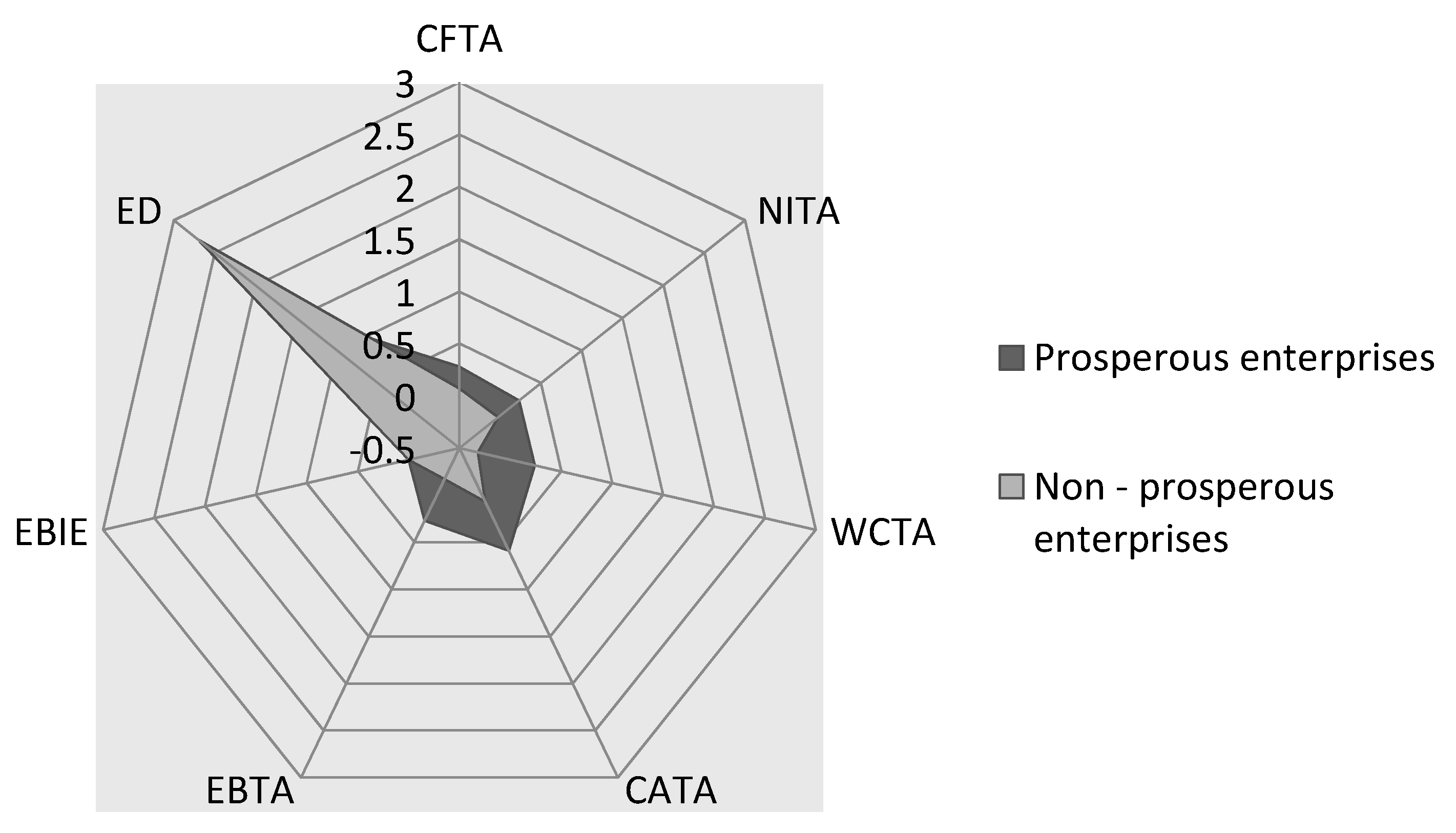
The financial distress frontier is formed by businesses that achieve relatively low values for inputs and at the same time relatively high values for outputs; these are businesses with a high probability of financial problems in the future. Regarding inputs, average profitability (NITA) is 2.6%, cash flow to total assets (CFTA) represents 7% and working capital to total assets (WCTA) is −31%. Comparison of the results of prosperous and non-prosperous businesses is shown in Figure 2.
The important output of the BCC DEA model is the proposal of peer units for inefficient businesses. These businesses are marked F40, F34, F89, F126, F236, and F132. They achieve high values of inputs and low values of outputs; therefore, they are reference DMUs for non-prosperous businesses (Table 3).
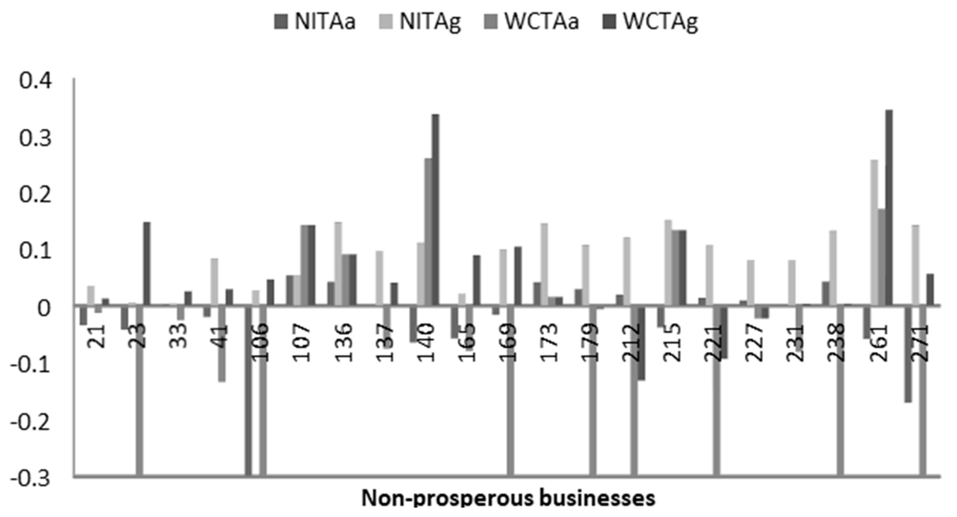
The greatest benefit of the DEA model is the calculation of goal values for inefficient DMUs that would make them efficient. Figure 3 shows selected inputs (NITA, WCTA) and their goal values for a group of non-prosperous businesses.
The goal values calculated in this way can be used as the starting point for the creation of a financial plan for non-prosperous businesses and compliance with them is a prerequisite for the future prosperity of these businesses.
To verify the results of the BCC model, we also applied the logit model. This model was formulated in Statistica using 5 indicators, which were selected according to the procedure described in Data and Methodology sections. Table 4 provides an estimate of the logit model coefficients. Based on this table, we can say that the statistically significant independent variables in the logit model are NITA, WCTA, and EBIE. These variables significantly contribute to the estimation accuracy of the logit model; the independent variable NITA has the greatest impact on the dependent variable.
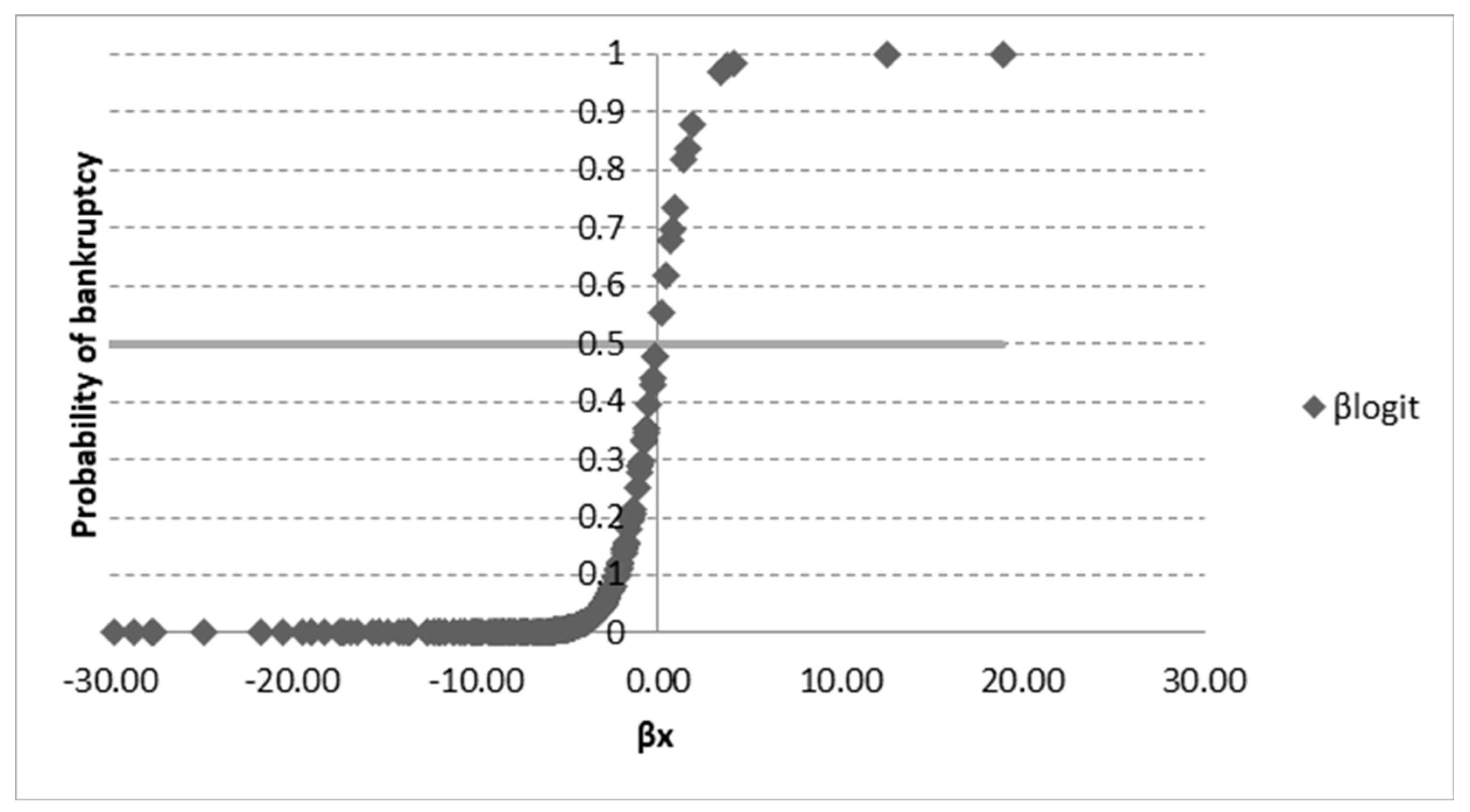
Figure 4 shows the distribution function of the logit model, which takes values in the range <0.1> and is symmetrical around the cut-off level 0.5. Businesses above the cut-off level are likely to fail, while those below the cut-off level are less likely (or not likely) to fail.
The p-value of the Hosmer–Lemeshow’s goodness of fit test is 0.9428. We do not reject the null hypothesis and state that there is no significant difference between the actual and predicted values of the dependent variable; the model is statistically significant and appropriate. The value of Nagelkerke’s R square is 0.6154, which means that the model explains 61.54% of the variability of the binary dependent variable.
To verify the estimation accuracy of the logit model, we chose the area under the curve (AUC) method, which measures the area under the receiver operating characteristic (ROC) curve. The AUC accounts for 0.9579; based on this, we can conclude that the logit model has very good estimation accuracy.
Based on the results presented in Table 5, the logit model correctly classified companies as non-prosperous or prosperous in 275 cases. This means that the model classified 265 businesses as prosperous, and based on the established criteria these businesses were actually considered prosperous. The model also classed 10 businesses as non-prosperous, whereby these businesses were actually considered non-prosperous. The model incorrectly classified 15 businesses. The estimation accuracy of the logit model is 45% for non-prosperous businesses and 99% for prosperous businesses.
Managerial Implications
This paper presents an empirical study on the application of the DEA method in the financial health evaluation of businesses from the Slovak heat industry. This empirical study contributes to the improvement of the financial health of these businesses by creating a suitable and easily applicable tool for financial health evaluation, as well as suggestions for improvement. It proposes goal values of inputs and outputs that determine the financial health of the analyzed sample. As DEA is a method that is not applied or is rarely applied in the management of Slovak companies, the findings of this study are expected to be very useful for managers and academics. From a theoretical point of view, the study offers and tests a dual DEA model for business financial health evaluation. It provides researchers and academics with a framework for examining factors that are important for the financial health of the company. It makes it possible to identify businesses that lie on financial health frontier as a pattern for other businesses. It is an excellent benchmarking tool to help businesses that do not lie on the financial health frontier to approach or even to reach it. Practical implementation of the DEA method is simple, thanks to the possibility of using MS Office, along with several software products that are processed for this area.
The application of the DEA method to the management of a company:
- ▪
- is significant for managing its efficiency as a part of operational management;
- ▪
- is an important part of its strategic management and a prerequisite for future growth, prosperity, and competitiveness;
- ▪
- identifies key efficiency indicators;
- ▪
- allows the use of multiple inputs and outputs;
- ▪
- is characterized by good data availability;
- ▪
- creates a benchmarking tool for comparing businesses and entire networks;
- ▪
- allows businesses to be ranked;
- ▪
- provides peer units and goal values;
- ▪
- allows lessons to be learned from successful businesses;
- ▪
- is easily applicable in practice.
5. Discussion
The results of the estimation accuracy for the DEA model are shown in Table 6. The estimation accuracy of the BCC model for non-prosperous businesses (sensitivity) is 41%. The estimation accuracy of this model for prosperous businesses (specificity) is 96%.
Results of the estimation accuracy achieved in our research can be compared with the results of previous studies. In one such study [104], the estimation accuracy for companies in financial distress was 24%, while the estimation accuracy of financially healthy businesses was 96.7%. There were also studies in which the classification ability of the DEA model for non-prosperous businesses was higher, such as [98], with classification ability of 10–42.86%; the work by [75], with classification ability of 84.89%; or the research by [73], who achieved classification ability of 74.4–75.7%.
In our research, we achieved 91% overall estimation accuracy of DEA model. In the studies by the above-mentioned authors, we can find similar or lower results for overall estimation accuracy of 75–77% [75], 88–95% [98], and 85.1–86.4% [73].
We examined the probability of bankruptcy using the DEA and logit models. According to [105,106], the above performance measures (accuracy, sensitivity, and specificity) depend on a certain cut-off value to label the class, which is generally set at 0.5. Therefore, we did not use them for the comparison of the results of the DEA and logit models. Instead, we applied a non-parametric Kolmogorov–Smirnov test to establish whether failed estimates from DEA and logit models differed significantly or not. The critical value is 0.08, which is less than the D-statistic value of 0.149466 (p-value = 0.001). Based on these results, we reject the null hypothesis of “no difference” or “same distribution”. The Kolmogorov–Smirnov test also reports that failure estimates are unlikely to come from the same distribution. We can conclude that each of these methods provides different and specific results. However, we consider the results of the DEA to be unique and will deal with them in more detail in further research.
Compared to statistical approaches, DEA has exceptional features; it does not need to meet certain statistical assumptions about the variables used in the model, it enables the processing of various inputs and outputs, quantifies the efficiency of each company separately, and determines the level of its efficiency in the form of a score. The great benefit of the DEA method is that it gives an answer to the question of how inefficient businesses can become inefficient. In this regard, DEA allows us to set goal values for inputs and outputs for inefficient businesses to become efficient and assigns businesses their peer units. Equally, this method does not consider initial conditions for non-prosperous businesses, rather its results are based on the achieved values of financial indicators, so they are independent of any assumptions.
The DEA model and the financial distress frontier are based on extreme values. This frontier captures only a small number of businesses. The disadvantages of the DEA model can be overcome by the application of a multistep DEA model, with the gradual elimination of businesses lying on the financial distress frontier. Another way of eliminating the problems arising from the application of the DEA model is to link the use of the financial health frontier and financial distress frontier, as well as to combine the DEA method with other prediction techniques, such as logistic regression.
Many researchers find the DEA model computationally difficult, however the availability of software solutions removes this problem. The challenge of the application of DEA models also relates to the selection of inputs and outputs. The discussions around the challenges of the DEA model imply that it is not clear yet whether these indicators should be absolute, relative, or combined. It is also necessary to perform a correlation analysis before the analysis itself in order to remove unnecessary redundancy in the variables. A significant problem with financial indicators is their negative value, which is not an unusual phenomenon in the case of profitability. When working with negative values, DEA models require a special approach or the application of an additive model.
6. Conclusions
Based on the research carried out in this paper, we can conclude that the DEA method is a suitable alternative for assessing the financial health of businesses from analyzed samples. Despite the fact that the logit model achieved higher estimation accuracy than the DEA model, it can only assess the probability that the company is financially healthy or that it fails. The important benefit of the DEA model is the frontier analysis. This allows us to identify financially healthy businesses that lie on the financial health frontier. These businesses represent patterns (peer units) from which the other businesses should learn. In this paper, we proposed peer units for inefficient businesses and also calculated goal values of individual inputs and outputs, which inefficient businesses should use in order to become efficient. Within the frontier analysis, we also identified businesses that are threatened by bankruptcy.
The BCC DEA model applied in this paper has relatively lower estimation accuracy for non-prosperous companies. However, the model has high estimation accuracy for prosperous companies. This can greatly influence the practical use of the DEA model. The low estimation accuracy of the DEA model in assessing the probability of bankruptcy is due to the fact that the DEA model and the financial distress frontier are based on extreme values. This limitation can be overcome by focusing on better preparation of inputs and outputs and by testing the selection of indicators to predict business failure, which will enter the DEA model. In our research, we tested variables used by [75]. Our future research will focus on the selection of a different set of indicators and their subsequent testing and comparison with the already implemented models. We will also pay more attention to selecting an appropriate database and to eliminating the effects of extreme values.
Author Contributions
Methodology, J.H. and M.M.; Resources, J.H. and M.M.; Software, J.H. and M.M.; Writing—original draft, J.H. and M.M. All authors have read and agreed to the published version of the manuscript.
Funding
This research received no external funding.
Acknowledgments
This paper was prepared within the grant scheme VEGA No. 1/0741/20 (the application of variant methods in detecting symptoms of possible bankruptcy of Slovak businesses in order to ensure their sustainable development).
Conflicts of Interest
The authors declare no conflict of interest.
References
- Denis, D.; Denis, D. Causes of Financial Distress Following Leveraged Recapitalizations. J. Financ. Econ. 1995, 37, 129–157. [Google Scholar] [CrossRef]
- Platt, H.; Platt, M. Predicting Corporate Financial Distress: Reflection on Choice—Based Sample Bias. J. Econ. Financ. 2002, 26, 184–199. [Google Scholar] [CrossRef]
- Balcaen, S.; Ooghe, H. 35 Years of Studies on Business Failure: An Overview of the Classic Statistical Methodologies and Their Related Problems. Br. Account. Rev. 2006, 38, 63–93. [Google Scholar] [CrossRef]
- Goldson, M. The Turnaround Prescription: Repositioning Troubled Companies; Free Press: New York, NY, USA, 1992. [Google Scholar]
- Michalková, L.; Valašková, K.; Frajtová Michalíková, K.; Drugau, A.C. The Holistic View of the Symptoms of Financial Health of Businesses. In Proceedings of the 3rd International Conference on Economic and Business Management (FEBM 2018), Honhot, China, 20–22 October 2018; Skitmore, M., Huang, X., Eds.; Atlantis Press: Paris, France, 2018. [Google Scholar]
- Geng, R.; Bose, I.; Chen, X. Prediction of financial distress: An empirical study of listed Chinese companies using data mining. Eur. J. Oper. Res. 2014, 241, 236–247. [Google Scholar] [CrossRef]
- Ding, Y.S.; Song, X.P.; Zen, Y.M. Forecasting Financial Condition of Chinese Listed Companies Based on Support Vector Machine. Expert Syst. Appl. 2008, 34, 3081–3089. [Google Scholar] [CrossRef]
- Klieštik, T. Predikcia Finančného Zdravia Podnikov Tranzitívnych Ekonomík; EDIS: Žilina, Slovakia, 2019. [Google Scholar]
- Dambolena, I.G.; Khoury, S.J. Ratio Stability and Corporate Failure. J. Financ. 1980, 35, 1017–1026. [Google Scholar] [CrossRef]
- Gombola, M.B.; Ketz, J.E. A note on cash flow and classification patterns of financial ratios. Account. Rev. 1983, 3, 105–114. [Google Scholar]
- Jo, H.; Han, I.; Lee, H. Bankruptcy prediction using case-based reasoning, neural networks and discriminant analysis. Expert Syst. Appl. 1997, 13, 97–108. [Google Scholar] [CrossRef]
- Scott, J. The probability of bankruptcy. A comparison of empirical predictions and theoretical models. J. Bank. Financ. 1981, 5, 317–344. [Google Scholar] [CrossRef]
- Chung, H.M.; Tam, K.Y. A comparative analysis of inductive learning algorithms. Intell. Syst. Account. Financ. Manag. 1993, 2, 3–18. [Google Scholar] [CrossRef]
- Jo, H.; Han, I. Integration of cased-based forecasting, neural network and discriminant analysis for bancruptcy prediction. Expert Syst. Appl. 1996, 11, 415–422. [Google Scholar] [CrossRef]
- Bešlić, D.; Jakšić, D.; Bešlić, I.; Andrić, M. Insolvency prediction model of the company: The case of the Republic of Serbia. Econ. Res. -Ekon. Istraživanja 2018, 31, 139–157. [Google Scholar] [CrossRef] [Green Version]
- Aziz, M.A.; Dar, H.A. Predicting corporate bankruptcy: Where we stand? Corp. Gov. 2006, 6, 18–33. [Google Scholar] [CrossRef] [Green Version]
- Araghi, K.; Makvandi, S. Evaluating Predictive power of Data Envelopment Analysis Technique Compared with logit and probit Models in Predicting Corporate Bankruptcy. Aust. J. Bus. Manag. Res. 2012, 2, pp. 38–46. Available online: https://pdfs.semanticscholar.org/8f45/3a426e86abf328e836bfbc9216eff2dac75d.pdf (accessed on 10 January 2019).
- Sun, J.; Li, H.; Huang, Q.H.; He, K.Y. Predicting Financial Distress and Corporate Failure: A Review from the State-of-the-art Definitions, Modeling, Sampling, and Featuring Approaches. Knowl.-Based Syst. 2014, 57, 41–56. [Google Scholar] [CrossRef]
- Mihalovič, M. Využitie skóringových modelov pri predikcii úpadku ekonomických subjektov v Slovenskej republike. Politická Ekon. 2018, 66, 689–708. [Google Scholar] [CrossRef] [Green Version]
- Beaver, W.H. Financial ratios as predictors of failure. J. Account. Res. 1966, 4, 71–111. [Google Scholar] [CrossRef]
- Šarlija, N.; Jeger, M. Comparing financial distress prediction models before and during recession. Croat. Oper. Res. Rev. 2011, 2, 133–142. [Google Scholar]
- Kidane, H.W. Predicting Financial Distress in IT and Services Companies in South Africa. Master’s Thesis, Faculty of Economics and Management Sciences, Bloemfontein, South Africa, 2004. Available online: http://scholar.ufs.ac.za:8080/xmlui/handle/11660/1117 (accessed on 18 June 2018).
- Spuchľáková, E.; Frajtová Michalíková, K. Comparison of LOGIT, PROBIT and neural network bankruptcy prediction models. In Proceedings of the 2016 ISSGBM International Conference on Information and Business Management, Hong Kong, China, 3–4 September 2016; Singapore Management and Sports Science Institute: Singapore, 2016. [Google Scholar]
- Altman, E.I. Financial Ratios, Discriminant Analysis and the Prediction of Corporate Bankruptcy. J. Financ. 1968, 23, 589–609. [Google Scholar] [CrossRef]
- Altman, E.I.; Haldeman, R.G.; Narayanan, P. ZETA ANALYSIS, a new model to identify bankruptcy risk of corporations. J. Bank. Financ. 1977, 1, 29–54. [Google Scholar] [CrossRef]
- Blum, M. Failing company discriminant analysis. J. Account. Res. 1974, 12, 1–25. [Google Scholar] [CrossRef]
- Deakin, E.B. A Discriminant Analysis of Predictors of Business Failure. J. Account. Res. 1972, 10, 167–179. [Google Scholar] [CrossRef]
- Elam, R. The effect of lease data on the predictive ability of financial ratios. Account. Rev. 1975, 5, 25–43. [Google Scholar]
- Norton, C.L.; Smith, R.E. A comparison of general price level and historical cost financial statemnets in the prediction of bankruptcy. Account. Rev. 1979, 54, 72–87. [Google Scholar]
- Wilcox, J.W. A prediction of business failure using accounting data. J. Account. Res. Sel. Stud. 1973, 11, 163–179. [Google Scholar] [CrossRef]
- Taffler, R.J. The assessment of company solvency and performance using a statistical model. Account. Bus. Res. 1983, 13, 295–308. [Google Scholar] [CrossRef]
- Cisko, S.; Klieštik, T. Finančný Manažment; Edis Publishing, University of Žilina: Žilina, Slovakia, 2013. [Google Scholar]
- Mihalovič, M. The Assessment of Corporate Financial Performance via Discriminant Analysis. Acta Oeconomica Cassoviensia Sci. J. 2015, 8, 57–69. [Google Scholar] [CrossRef]
- Klieštik, T.; Majerová, J.; Lyakin, A.N. Metamorphoses and Semantics of Corporate Failures as a Basal Assumption of a Well-founded Prediction of a Corporate Financial Health. In Proceedings of the 3rd International Conference on Economics and Social Science ICESS 2015, Changsha, China, 28–29 December 2015; Lee, G., Ed.; Volume 86, pp. 150–154. [Google Scholar]
- Gundová, P. Verification of the selected prediction methods in Slovak companies. Acta Acad. Karviniensia 2015, 14, 26–38. [Google Scholar] [CrossRef] [Green Version]
- Martin, D. Early warning of bank failure. A logit regression approach. J. Bank. Financ. 1977, 1, 249–276. [Google Scholar] [CrossRef]
- Ohlson, J. Financial ratios and the probabilistic prediction of bankruptcy. J. Account. Res. 1980, 18, 109–131. [Google Scholar] [CrossRef] [Green Version]
- Kliestik, T.; Lyakin, A.N.; Valaskova, K. Stochastic calculus and modelling in economics and finance. In Proceedings of the 2nd International Conference on Economics and Social Science ICESS 2014, Shenzhen, China, 29–30 July 2014; Lee, G., Ed.; pp. 161–167. [Google Scholar]
- Mišanková, M.; Spuchľáková, E.; Frajtová-Michalíková, K. Determination of Default Probability by Loss Given Default. Procedia Econ. Financ. 2015, 26, 411–417. [Google Scholar] [CrossRef]
- Gloubos, G.; Grammatikos, T. The success of bankruptcy prediction models in Greece. Stud. Bank. Financ. 1988, 7, 37–46. [Google Scholar]
- Zmijewski, M. Methodological issues related to the estimation of financial distress prediction models. J. Account. Res. 1984, 22, 59–82. [Google Scholar] [CrossRef]
- Albright, J. What Is the Difference Between Logit and Probit Models? 2015. Available online: https://www.methodsconsultants.com/tutorial/what-is-the-difference-between-logit-and-probit-models/ (accessed on 1 January 2019).
- Adamko, P.; Švábová, L. Prediction of the risk of bankruptcy of Slovak companies. In Proceedings of the 8th International Scientific Conference on Managing and Modelling of Financial Risks, Ostrava, Czech Republic, 5–6 September 2016; VSB-Technical University: Ostrava, Czech Republic, 2016; pp. 15–20. Available online: https://www.ekf.vsb.cz/export/sites/ekf/rmfr/cs/sbornik/Soubory/Part_I.pdf (accessed on 10 July 2019).
- Jakubík, P.; Teplý, P. The Prediction of Corporate Bankruptcy and Czech Economy’s Financial Stability through Logit Analysis; IES Working Paper 19/2008; IES FSV, Univerzita Karlova: Prague, Czech Republic, 2008; Available online: https://www.econstor.eu/bitstream/10419/83366/1/578585421.pdf (accessed on 10 September 2019).
- Valecký, J.; Slivková, E. Microeconomic Scoring Model of Czech Firms’ Bankruptcy. Ekonomická Revue 2012, 15, 15–26. [Google Scholar]
- Hand, D.J. Artificial Intelligence and Psychiatry; Cambridge University Press: Cambridge, UK, 1985. [Google Scholar]
- Nath, R.; Jackson, W.M.; Jones, T.W. A Comparison of the Classical and the Linear Programming Approaches to the Classification Problem in Discriminant Analysis. J. Stat. Comput. Simul. 1992, 41, 73–93. [Google Scholar] [CrossRef]
- Horváthová, J.; Mokrišová, M. Risk of Bankruptcy, its Determinants and Models. Risks. 2018, 6, 117. [Google Scholar] [CrossRef] [Green Version]
- Štefko, R.; Gavurová, B.; Kočišová, K. Healthcare efficiency assessment using DEA analysis in the Slovak Republic. Health Econ. Rev. 2018, 8, 1–12. [Google Scholar] [CrossRef]
- Charnes, A.; Cooper, W.W.; Rhodes, E. Measuring the efficiency of decision making units. Eur. J. Oper. Res. 1978, 2, 429–444. [Google Scholar] [CrossRef]
- Farrell, M.J. The Measurement of Productive Efficiency. J. R. Stat. Soc. Ser. A 1957, 120, 253–290. [Google Scholar] [CrossRef]
- Debreu, G. The coefficient of resource utilization. Econometrica 1951, 19, 273–292. [Google Scholar] [CrossRef]
- Koopmans, T.C. Analysis of production as an efficient combination of activities. In Activity Analysis of Production and Allocation; Koopmans, T.C., Ed.; John Wiley and Sons Inc.: Hoboken, NJ, USA, 1951; pp. 33–97. [Google Scholar]
- Banker, R.D.; Charnes, A.; Cooper, W.W. Some models for estimating technical and scale inefficiencies in data envelopment analysis. Manag. Sci. 1984, 30, 1078–1092. [Google Scholar] [CrossRef] [Green Version]
- Färe, R.; Grosskopf, S.; Lovell, C.A. Measurement of Efficiency of Production; Kluwer-Nijhoff Publishing Co.: Boston, MA, USA, 1985. [Google Scholar]
- Zhu, J. DEA Based Benchmarking Models. In Data Envelopment Analysis. International Series in Operations Research & Management Science; Zhu, J., Ed.; Springer: Berlin/Heidelberg, Germany, 2015; Volume 221, pp. 291–308. [Google Scholar]
- Tone, K. A slacks-based measure of efficiency in data envelopment analysis. Eur. J. Oper. Res. 2001, 130, 498–509. [Google Scholar] [CrossRef] [Green Version]
- Färe, R.; Grosskopf, S.; Margaritis, D. Advances in Data Envelopment Analysis; World Scientific Books; World Scientific Publishing Co. Pte. Ltd.: Singapore, 2015. [Google Scholar]
- Wang, Y.M.; Chin, K.S.; Yang, J.B. Measuring the performances of decision-making units using geometric average efficiency. J. Oper. Res. Soc. 2007, 58, 929–937. [Google Scholar] [CrossRef]
- Sexton, T.R.; Silkman, R.H.; Hogan, A.J. Data Envelopment Analysis: Critique and Extensions. In Measuring Efficiency: An Assessment of Data Envelopment Analysis; Jossey-Bass: San Francisco, CA, USA, 1986; Volume 1986, pp. 73–105. [Google Scholar]
- Kao, C.; Hwang, S.N. Efficiency decomposition in twostage data envelopment analysis: An application to non-life insurance companies in Taiwan. Eur. J. Oper. Res. 2008, 185, 418–429. [Google Scholar] [CrossRef]
- Paradi, J.C.; Rouatt, S.; Zhu, H. Two-stage evaluation of bank branch efficiency using data envelopment analysis. Omega 2011, 39, 99–109. [Google Scholar] [CrossRef]
- Johnes, J. Data envelopment analysis and its application to the measurement of efficiency in higher education. Econ. Educ. Rev. 2006, 25, 273–288. [Google Scholar] [CrossRef] [Green Version]
- Thanassoulis, E. Introduction to the Theory and Application of Data Envelopment Analysis; Springer: New York, NY, USA, 2001. [Google Scholar]
- Thrall, R.M. What Is the Economic Meaning of FDH? J. Product. Anal. 1999, 11, 243–250. [Google Scholar] [CrossRef]
- Sadjadi, S.J.; Omrani, H. Data envelopment analysis with uncertain data: An application for Iranian electricity distribution companies. Energy Policy 2008, 36, 4247–4254. [Google Scholar] [CrossRef]
- Hafezalkotob, A.; Haji-Sami, E.; Omrani, H. Robust DEA under discrete uncertain data: A case study of Iranian electricity distribution companies. J. Ind. Eng. Int. 2015, 11, 199–208. [Google Scholar] [CrossRef] [Green Version]
- Ferrier, G.D.; Rosko, M.D.; Valdmanis, V.G. Analysis of uncompensated hospital care using a DEA model of output congestion. Health Care Manag. Sci. 2006, 9, 181–188. [Google Scholar] [CrossRef]
- Bawa, S.; Ruchita, R. Efficiencies of health insurance business in India: An application of DEA. Am. J. Soc. Manag. Sci. 2011, 2, 237–247. [Google Scholar] [CrossRef]
- Jakovljevic, M.B.; Vukovic, M.; Fontanesi, J. Life expectancy and health expenditure evolution in Eastern Europe—DiD and DEA analysis. Expert Rev. Pharm. Outcomes Res. 2016, 16, 537–546. [Google Scholar] [CrossRef]
- Thabrani, G.; Irfan, M.; Mesta, H.A.; Arifah, L. Efficiency Analysis of Local Government Health Service in West Sumatra Province Using Data Envelopment Analysis (DEA). In Proceedings of the 1st International Conference on Economics, Business, Entrepreneurship, and Finance (ICEBEF 2018), Bandung, Indonesia, 19 September 2018; Atlantis Press: Paris, France, 2019; pp. 783–789. [Google Scholar]
- Simak, P.C. DEA Based Analysis of Coporate Failure. Master’s Thesis, Faculty of Applied Sciences and Engineering, University of Toronto, Toronto, ON, Canada, 1997. [Google Scholar]
- Cielen, A.; Peeters, L.; Vanhoof, K. Bankruptcy prediction using a data envelopment analysis. Eur. J. Oper. Res. 2004, 154, 526–532. [Google Scholar] [CrossRef]
- Paradi, J.C.; Asmild, M.; Simak, P.C. Using DEA and worst practice DEA in credit risk evaluation. J. Product. Anal. 2004, 21, 153–165. [Google Scholar] [CrossRef]
- Premachandra, I.M.; Bhabra, G.S.; Sueyoshi, T. DEA as a tool for bankruptcy assessment: A comparative study with logistic regression technique. Eur. J. Oper. Res. 2009, 193, 412–424. [Google Scholar] [CrossRef]
- Sueyoshi, T.; Goto, M. Methodological comparison between DEA and DEA-DA from the perspective of bankruptcy assessment. Eur. J. Oper. Res. 2009, 188, 561–575. [Google Scholar] [CrossRef]
- Premachandra, I.M.; Chen, Y.; Watson, J. DEA as a Tool for Predicting Corporate Failure and Success: A Case of Bankruptcy Assessment. Omega 2011, 3, 620–626. [Google Scholar] [CrossRef]
- Shetty, U.; Pakkala, T.; Mallikarjunappa, T. A modified directional distance formulation of DEA to assess bankruptcy: An application to IT/ITES companies in India. Expert Syst. Appl. 2012, 9, 1988–1997. [Google Scholar] [CrossRef]
- Roháčová, V.; Kráľ, P. Corporate failure prediction using DEA: An application to companies in the Slovak Republic. In Proceedings of the 18th International Scientific Conference Applications of Mathematics and Statistics in Economics (AMSE), Jindřichúv Hradec, Czech Republic, 2–6 September 2015; Hronová, S., Vltavská, K., Eds.; Oeconomica Publishing House, University of Economics: Prague, Czech Republic, 2015. Available online: http://amse-conference.eu/history/amse2015/doc/Rohacova_Kral.pdf (accessed on 30 October 2019).
- Vavřina, J.; Hampel, D.; Janová, J. New approaches for the financial distress classification in agribusiness. Acta Univ. Agric. Silvic. Mendel. Brun. 2013, 61, 1177–1182. [Google Scholar] [CrossRef] [Green Version]
- Visani, F.; Barbieri, P.; Di Lascio, F.M.L.; Raffoni, A.; Vigo, D. Supplier’s total cost of ownership evaluation: A data envelopment analysis approach. Omega 2016, 61, 141–154. [Google Scholar] [CrossRef] [Green Version]
- Wanke, P.; Azad, M.A.K.; Emrouznejad, A.; Antunes, J. A dynamic network DEA model for accounting and financial indicators: A case of efficiency in MENA banking. Int. Rev. Econ. Financ. 2019, 61, 52–68. [Google Scholar] [CrossRef] [Green Version]
- Gherghina, S.C. An Artificial Intelligence Approach towards Investigating Corporate Bankruptcy. Rev. Eur. Stud. 2015, 7, 5–22. [Google Scholar] [CrossRef] [Green Version]
- Altman, E.I.; Marco, G.; Varetto, F. Corporate distress diagnosis: Comparisons using linear discriminant analysis and neural networks (the Italian experience). J. Bank. Financ. 1994, 18, 505–529. [Google Scholar] [CrossRef]
- Atiya, A.F. Bankruptcy prediction for credit risk using neural networks: A survey and new results. IEEE Trans. Neural Netw. 2001, 12, 929–935. [Google Scholar] [CrossRef] [PubMed] [Green Version]
- Abid, F.; Zouari, A. Predicting corporate financial distress: A new neural networks approach. Financ. India 2002, 16, 601–612. [Google Scholar]
- Du Jardin, P. Predicting bankruptcy using neural networks and other classification methods: The influence of variable selection techniques on model accuracy. Neurocomputing 2010, 73, 2047–2060. [Google Scholar] [CrossRef] [Green Version]
- Zouari, A. Discriminating Firm Financial Health Using Self-Organizing Maps: The Case of Saudi Arabia; Department of Finance and Investment, College of Economics and Administrative Sciences, Imam Muhammad Bin Saud Islamic University: Riyadh, Saudi Arabia, 2012. [Google Scholar]
- CRIF. Financial Statements of Businesses; Slovak Credit Bureau, s.r.o.: Bratislava, Slovakia, 2016. [Google Scholar]
- Csikósová, A.; Janošková, M.; Čulková, K. Limitation of Financial Health Prediction in companies from Post-Communist Countries. J. Risk Financ. Manag. 2019, 12, 15. [Google Scholar] [CrossRef] [Green Version]
- Kočišová, K. Technical efficiency of top 50 world banks. J. Appl. Econ. Sci. 2013, 8, 311–322. [Google Scholar]
- Kočišová, K. Aplikácia DEA modelov pri analýze technickej efektívnosti pobočiek komerčnej banky. Ekonomický Časopis 2012, 60, 169–186. [Google Scholar]
- Barišic, P.; Cvetkoska, V. Analyzing the Efficiency of Travel and Tourism in the European Union. In Advances in Operational Research in the Balkans, Proceedings of the 13th Balkan Conference on Operational Research, Belgrade, Serbia, 25–28 May 2018; Mladenovic, N., Sifaleras, A., Kuxmanovic, M., Eds.; Elsevier: Amsterdam, The Netherlands, 2020; pp. 167–186. [Google Scholar]
- Altman, E.I. Corporate Financial Distress. A Complete Guide to Predicting, Avoiding, and Dealing with Bankruptcy; Wiley Interscience, John Wiley and Sons: Hoboken, NJ, USA, 1983. [Google Scholar]
- Klieštik, T. Kvantifikácia efektivity činností dopravných podnikov pomocou Data Envelopment Analysis. E+M Ekon. Manag. 2009, 1, 133–145. [Google Scholar]
- Vincová, K. Využitie DEA modelov na hodnotenie efektívnosti. Biatec 2005, 13, 24–28. [Google Scholar]
- Kováčová, M.; Klieštik, T. logit and probit application for the prediction of bankruptcy in Slovak companies. Equilib. Q. J. Econ. Econ. Policy 2017, 12, 775–791. [Google Scholar] [CrossRef]
- Mendelová, V.; Stachová, M. Comparing DEA and logistic regression in corporate financial distress prediction. In Proceedings of the International Scientific Conference FERNSTAT 2016, Banská Bystrica, Slovakia, 22–23 September 2016; Boďa, M., Ed.; Slovak Statistical and Demographic Society: Banská Bystrica, Slovakia, 2016; pp. 95–104. Available online: http://fernstat.ssds.sk/proceedings/ (accessed on 10 November 2019).
- Valášková, K.; Švábová, L.; Ďurica, M. Verifikácia predikčných modelov v podmienkach slovenského poľnohospodárskeho sektora. Ekon. Manag. Inovace 2017, 9, 30–38. [Google Scholar]
- Boďa, M.; Úradníček, V. The portability of Altman’s Z-score model to predicting corporate financial distress of Slovak companies. Technol. Econ. Dev. Econ. 2016, 22, 532–553. [Google Scholar] [CrossRef] [Green Version]
- Sperandei, S. Understanding logistic regression analysis. Biochem. Med. 2014, 24, 12–18. [Google Scholar] [CrossRef] [PubMed]
- Hebák, J. Statistické Myšlení a Nástroje Analýzy Dat; Informatorium: Prague, Czech Republic, 2015. [Google Scholar]
- Zhu, J. DEA Frontier Software; Foisie Business School, Worcester Polytechnic Institute: Worcester, MA, USA, 2019. [Google Scholar]
- Mendelová, V.; Bieliková, T. Diagnostikovanie finančného zdravia podnikov pomocou metódy DEA: Aplikácia na podniky v Slovenskej republike. Politická Ekon. 2017, 65, 26–44. [Google Scholar] [CrossRef] [Green Version]
- Ling, C.X.; Huang, J.; Zhang, H. AUC: A statistically consistent and more discriminating measure than accuracy. In Proceedings of the International Joint Conferences on Artificial Intelligence, Acapulco‚ Mexico‚, 9−15 August 2003; pp. 519–526. Available online: https://cling.csd.uwo.ca/papers/ijcai03.pdf (accessed on 8 March 2020).
- Anouze, A.L.M.; Bou-Hamad, I. Data envelopment analysis and data mining to efficiency estimation and evaluation. Int. J. Islamic Middle East. Financ. Manag. 2019, 12, 169–190. [Google Scholar] [CrossRef] [Green Version]
Figure 1.
Flowchart of the research. DEA, data envelopment analysis.

Figure 2.
Comparison of selected indicators. Abbreviations: cash flow/total assets, CFTA; net income/total assets, NITA; working capital/total assets, WCTA; current assets/total assets, CATA; earnings before interest and taxes/total assets, EBTA; earnings before interest and taxes/interest expenses, EBIE; equity/debt, ED.

Figure 3.
Goal values of selected parameters for non-prosperous businesses. Legend: a, actual; g, goal.
Figure 3.
Goal values of selected parameters for non-prosperous businesses. Legend: a, actual; g, goal.

Figure 4.
Distribution function of the logit model.


Table 1.
Efficient businesses analyzed with the BCC DEA model.
| Input-Oriented | |||
|---|---|---|---|
| BCC Model | |||
| DMU Name | Efficiency | Benchmarks | |
| F34 | 1.00000 | 1.000 | F34 |
| F40 | 1.00000 | 1.000 | F40 |
| F89 | 1.00000 | 1.000 | F89 |
| F91 | 1.00000 | 1.000 | F91 |
| F101 | 1.00000 | 1.000 | F101 |
| F120 | 1.00000 | 1.000 | F120 |
| F132 | 1.00000 | 1.000 | F132 |
| F139 | 1.00000 | 1.000 | F139 |
| F147 | 1.00000 | 1.000 | F147 |
| F156 | 1.00000 | 1.000 | F156 |
| F161 | 1.00000 | 1.000 | F161 |
| F236 | 1.00000 | 1.000 | F236 |
| F250 | 1.00000 | 1.000 | F250 |
| F254 | 1.00000 | 1.000 | F254 |
| F269 | 1.00000 | 1.000 | F269 |
| F288 | 1.00000 | 1.000 | F288 |
Source: authors of [103], processed in DEAFrontier software.
Table 2.
Businesses on the financial distress frontier analyzed with the BCC DEA model.
| Input-Oriented | |||
|---|---|---|---|
| BCC Model | |||
| DMU Name | Efficiency | Benchmarks | |
| F23 | 1.00000 | 1.000 | F23 |
| F33 | 1.00000 | 1.000 | F33 |
| F41 | 1.00000 | 1.000 | F41 |
| F88 | 1.00000 | 1.000 | F88 |
| F106 | 1.00000 | 1.000 | F106 |
| F107 | 1.00000 | 1.000 | F107 |
| F136 | 1.00000 | 1.000 | F136 |
| F137 | 1.00000 | 1.000 | F137 |
| F140 | 1.00000 | 1.000 | F140 |
| F165 | 1.00000 | 1.000 | F165 |
| F169 | 1.00000 | 1.000 | F169 |
| F173 | 1.00000 | 1.000 | F173 |
| F179 | 1.00000 | 1.000 | F179 |
| F212 | 1.00000 | 1.000 | F212 |
| F215 | 1.00000 | 1.000 | F215 |
| F221 | 1.00000 | 1.000 | F221 |
| F227 | 1.00000 | 1.000 | F227 |
| F231 | 1.00000 | 1.000 | F231 |
| F238 | 1.00000 | 1.000 | F238 |
| F261 | 1.00000 | 1.000 | F261 |
| F271 | 1.00000 | 1.000 | F271 |
Source: authors of [103], processed in DEAFrontier software.
Table 3.
Reference DMUs.
| BCC DEA | Peer Units for DMUs | |||||||||
|---|---|---|---|---|---|---|---|---|---|---|
| VRS | ||||||||||
| DMU No. | DMU Name | Efficiency | ||||||||
| 23 | F23 | 1.23075 | 0.190 | F40 | 0.061 | F89 | 0.748 | F126 | ||
| 33 | F33 | 1.14391 | 0.640 | F34 | 0.201 | F40 | 0.159 | F236 | ||
| 41 | F41 | 1.18367 | 0.181 | F40 | 0.146 | F89 | 0.143 | F126 | 0.530 | F288 |
| 88 | F88 | 1.15604 | 0.099 | F34 | 0.211 | F40 | 0.690 | F132 | ||
| 106 | F106 | 1.19726 | 0.122 | F40 | 0.874 | F126 | 0.004 | F156 | ||
| 107 | F107 | 1.13749 | 0.198 | F40 | 0.073 | F91 | 0.730 | F132 | ||
| 136 | F136 | 1.06418 | 0.093 | F40 | 0.022 | F236 | 0.709 | F250 | 0.176 | F254 |
| 137 | F137 | 1.19797 | 0.270 | F40 | 0.002 | F126 | 0.728 | F132 | ||
| 140 | F140 | 1.10508 | 0.084 | F40 | 0.177 | F126 | 0.739 | F132 | ||
| 165 | F165 | 1.16846 | 0.143 | F40 | 0.429 | F126 | 0.428 | F132 | ||
| 169 | F169 | 1.16080 | 0.051 | F40 | 0.514 | F89 | 0.436 | F126 | ||
| 173 | F173 | 1.14813 | 0.446 | F34 | 0.238 | F40 | 0.316 | F132 | ||
| 179 | F179 | 1.18514 | 0.142 | F40 | 0.268 | F89 | 0.589 | F126 | ||
| 212 | F212 | 1.22325 | 0.182 | F40 | 0.482 | F89 | 0.336 | F126 | ||
| 215 | F215 | 1.11866 | 0.598 | F34 | 0.159 | F40 | 0.244 | F132 | ||
| 221 | F221 | 1.21425 | 0.134 | F40 | 0.809 | F89 | 0.058 | F126 | ||
| 227 | F227 | 1.14343 | 0.740 | F34 | 0.241 | F40 | 0.020 | F132 | ||
| 231 | F231 | 1.18273 | 0.244 | F40 | 0.160 | F126 | 0.597 | F132 | ||
| 238 | F238 | 1.18128 | 0.112 | F40 | 0.640 | F89 | 0.248 | F126 | ||
| 261 | F261 | 1.10447 | 0.040 | F40 | 0.478 | F126 | 0.482 | F132 | ||
| 271 | F271 | 1.24384 | 0.043 | F40 | 0.956 | F89 | 0.001 | F156 | ||
Source: authors of [103], processed in DEAFrontier software.
Table 4.
Logit function coefficients.
| Parameter | Estimate | Standard Error | Wald stat. | Lower and Upper Confidence Limit 95.0% | p-Value | |
|---|---|---|---|---|---|---|
| Intercept | −0.9778 | 0.77374 | 1.59710 | −2.4943 | 0.5387 | 0.206315 |
| NITA | −40.9544 | 12.48770 | 10.75566 | −65.4299 | −16.4790 | 0.001040 |
| WCTA | −6.1530 | 1.89538 | 10.53842 | −9.8679 | −2.4381 | 0.001169 |
| EBIE | −1.4028 | 0.50667 | 7.66528 | −2.3958 | −0.4097 | 0.005629 |
| ED | 0.0653 | 0.13258 | 0.24270 | −0.1945 | 0.3252 | 0.622262 |
| CLTA | −1.0043 | 1.58714 | 0.40041 | −4.1150 | 2.1064 | 0.526875 |
Source: authors. Processed in Statistica software.
Table 5.
Estimation accuracy of the logit model, with a cut-off point equal to 0.5.
| Predicted Value: Non-prosperous | Correct Percentage | |||
|---|---|---|---|---|
| Yes | No | |||
| Observed value: Non-prosperous | Yes | 10 | 12 | 45 |
| No | 3 | 265 | 99 | |
Source: authors. Processed in Statistica software.
Table 6.
Comparison of the estimation accuracy of the BCC model and the logit model.
| Parameter | BCC Model | Logit Model |
|---|---|---|
| Sensitivity (%) | 41 | 45 |
| Specificity (%) | 96 | 99 |
| Overall estimation accuracy (%) | 91 | 95 |
| Error type 1 (%) | 59 | 55 |
| Error type II (%) | 4 | 1 |
© 2020 by the authors. Licensee MDPI, Basel, Switzerland. This article is an open access article distributed under the terms and conditions of the Creative Commons Attribution (CC BY) license (http://creativecommons.org/licenses/by/4.0/).
Share and Cite
MDPI and ACS Style
Horváthová, J.; Mokrišová, M. Comparison of the Results of a Data Envelopment Analysis Model and Logit Model in Assessing Business Financial Health. Information 2020, 11, 160. https://doi.org/10.3390/info11030160
AMA Style
Horváthová J, Mokrišová M. Comparison of the Results of a Data Envelopment Analysis Model and Logit Model in Assessing Business Financial Health. Information. 2020; 11(3):160. https://doi.org/10.3390/info11030160
Chicago/Turabian StyleHorváthová, Jarmila, and Martina Mokrišová. 2020. "Comparison of the Results of a Data Envelopment Analysis Model and Logit Model in Assessing Business Financial Health" Information 11, no. 3: 160. https://doi.org/10.3390/info11030160
Note that from the first issue of 2016, this journal uses article numbers instead of page numbers. See further details here.