On the Randomness of Compressed Data

Abstract

It seems reasonable to expect from a good compression method that its output should not be further compressible, because it should behave essentially like random data. We investigate this premise for a variety of known lossless compression techniques, and find that, surprisingly, there is much variability in the randomness, depending on the chosen method. Arithmetic coding seems to produce perfectly random output, whereas that of Huffman or Ziv-Lempel coding still contains many dependencies. In particular, the output of Huffman coding has already been proven to be random under certain conditions, and we present evidence here that arithmetic coding may produce an output that is identical to that of Huffman.

1. Introduction

Research on lossless data compression has evolved over the years from various encoding variants, for instance [1,2,3,4,5,6,7], passing by more advanced challenges such as compressed pattern matching in texts [8,9], in images [10,11] and in structured files [12,13], and up to compact data structures [14,15,16,17].

The declared aim of lossless data compression is to recode some piece of information into fewer bits than given originally. This is often possible because the standard way we use to convey information has not been designed to be especially economical. In particular, natural language texts contain many redundancies that might enrich our spoken or written communication, but are not really necessary for the data to be complete and accurate. Many of these redundancies are kept for historical reasons, like double letters in many languages, or multiple letters representing a single sound, like sch in German or aient in French. There are also more subtle redundancies, like encoding all the characters with some fixed length code, whereas some letters are more frequent than others, which could be exploited by assigning them shorter codewords. Indeed, Huffman calls the code he designed in his seminal paper [1] a minimum-redundancy code.

It is therefore natural to assume that once as much redundancy as possible has been removed, the remaining text should be indistinguishable from random data, for if some more regularities can be detected, they could be targeted in an additional round of compression. Indeed, Fariña et al. [18] focus on byte-oriented word based compressors for natural languages, and show that such compressed files can be further compressed using any general purpose compressor such as gzip. They note that the frequencies of the byte values generated by a byte-oriented, word based, compressor, are far from uniform, as opposed to the output of arithmetic coding. They show how re-compressing word based encodings by standard compressors can be extended to compressed self-indices, because any character based self-index, such as compressed suffix arrays [19,20,21], can be directly constructed over the byte-oriented word based compressed file, without modification.

This paper extends this work and investigates several known compression techniques from the point of view of the randomness of their output. As will be shown, the a priori assumption that compressed output is perfectly random, is not necessarily true in all cases.

Beside the theoretical value of this research, it may have some important practical implications. Consider, for example, the possibility to use a compression scheme also as an encryption method, based on the fact that both compression and encryption try to eliminate redundancies, albeit for different reasons [22]. If compressed output is then indeed random, then any compression method could, in principle, also be used for data encryption, if the parameters on which the decoding depends, can be hidden from the decoder [23].

For instance, a Huffman encoded file will not be very useful unless the decoder knows how each of the characters has been encoded. If the encoding, and moreover, the set itself of the elements that have been encoded, can be kept secret, decoding might be difficult, as it would be equivalent to breaking the code, that is, guessing the codewords [24,25].

Another implication of a non-uniform output would be the possibility to apply another layer of compression to the compressed output itself. Consider the following simple example. Suppose a file F has been compressed into $C\left(F\right)$, which is not random because, say, the probability of a 1-bit in it is $p\ne \frac{1}{2}$. We could then apply an arithmetic coder to the individual bits of $C\left(F\right)$; arithmetic coding reaches the entropy so that the average number of bits required to encode a bit of $C\left(F\right)$ would be $-p{log}_{2}p-(1-p){log}_2(1-p)$, which is strictly smaller than 1 for $p\ne \frac{1}{2}$. For example, if $p=0.56$, the entropy would be 0.99, so the additional compression is able to reduce the size of the already compressed file by an additional percent.

The question of how to measure randomness has been treated in many different areas, in particular to check the validity of pseudo-random number generators. Many tests have been devised, for example, in Reference [26], to mention just a software library containing a collection of such tests. Chang et al. report on a series of experiments in References [27,28]. We shall rely on the notion of a binary sequence being m-distributed, due to Knuth [29], meaning that the probability of occurrence of every subtring of the input of length m is equal to $2^{-m}$. Knuth then goes on to define, in Definition R1, a sequence to be “random” if it is ∞-distributed, that is, m-distributed for all $m\ge 1$, and we shall approximate this with values $m\le 8$.

In the next section, we consider several known compression methods and discuss the randomness of their output. Section 3 then reports on some empirical tests, and Section 4 concludes.

2. Randomness of Compression Methods

2.1. Huffman Coding

One of the oldest compression methods is due to Huffman [1]. Given an alphabet $A=\{a_1,\dots ,a_n\}$ and a probability distribution $P=\{p_1,\dots ,p_n\}$ of its letters, the problem is to find a prefix code with codewords lengths $L=\{{\ell }_1,\dots ,{\ell }_n\}$ such that the weighted average length of a codeword, ${\sum }_{i=1}^n{p}_i{\ell }_i$, is minimized. Huffman’s algorithm finds a set L which is optimal under the constraints that the ${\ell }_i$ are all integers, and that the partition of the file to be compressed into elements to be encoded, or, equivalently, the alphabet A, is known and fixed throughout the process.

At first sight, a file compressed by means of a Huffman code seems to be very far from what one could consider as a random string. The code is a finite set of short binary strings which remain fixed once the code is chosen, and which serve as building blocks to construct the compressed file by concatenating the same strings time and again, though in varying order. One might therefore expect that the probability of occurrence of the strings representing codewords is larger than the probability of other strings of the same length. For example, a Huffman code could be $C=\{00,01,100,101,110,111\}$, and it is not self evident that a long string obtained by repeated concatenations of elements of the small set C will contain, say, the substring 00000 with probability $2^{-5}$.

Nevertheless, it has been shown in Reference [30] that the compressed file is random if the appearances of the elements in the text are independent of each other, and the probability distribution P is dyadic, that is, all the $p_i$ are powers of $\frac{1}{2}$. In other words, even though the distribution of binary strings of different lengths within the set of codewords is often very far from uniform, one has to take into account the probabilities of the occurrences of these strings, and these exactly counterbalance the apparent bias. In fact, even if the conditions are only partially met, the resulting file seems quite close to random in empirical tests. Indeed, suppose Huffman’s algorithm is applied on a non-dyadic distribution P, resulting in a length vector L. Then $P^{\prime }=\{2^{-{\ell }_1},\dots ,2^{-{\ell }_n}\}$ is a dyadic distribution yielding the same Huffman tree as P, which means that P and $P^{\prime }$ are "close" to each other in a certain sense. A measure of this closeness has been proposed in Reference [31].

As to the independence assumption, it is quite clear that if just a simple model is used, this assumption does not always hold, especially for natural text. For instance, it is not true that there is no dependence between the occurrence of consecutive single characters, say, in English texts: q is almost always followed by u, and the bigram ea is much more frequent than ae. However, such obvious dependencies can be circumvented, by incorporating them into an extended alphabet, as proposed in Reference [32]. Thus, if one encodes, for example, words or even phrases instead of individual characters, the elements will be less dependent, and moreover, compression will be improved.

Therefore, even though the strict mathematical conditions required for proving the randomness of the output of Huffman coding in Reference [30], as well as that of arithmetic coding in the following section, seem to be unlikely to occur in practice, they are nevertheless approximated in many real situations, as supported by our empirical results.

2.2. Arithmetic Coding

If one relaxes the constraint that all the codeword lengths ${\ell }_i$ have to be integers, then an optimal assignment of lengths, given the same problem as above with a probability distribution P as input, would be ${\ell }_i=-log{p}_i$, and the average codeword length would then be $-{\sum }_{i=1}^n{p}_{i}log{p}_i$, called the entropy. This can be reached by applying arithmetic coding [33].

Arithmetic coding represents the compressed text by a real number in a sub interval $[\ell ,h)$ of $[0,1)$. The interval is initialized by $[0,1)$, and each symbol $a_i$ narrows the current interval with respect to its probability. Formally, the interval $[\ell ,h)$ is partitioned into n subintervals, each corresponding to one of the characters $a_i\in A$. The size of a subinterval is proportional to the probability $p_i$ of the corresponding character $a_i$. For example, if $A=\left\{\mathsf{a},\mathsf{b},\mathsf{c}\right\}$ and the probabilities are $P=\{0.2,0.5,0.3\}$, then one possible partition could be $\left\{\right[0,0.2),[0.2,0.7),[0.7,1\left)\right\}$; if the text to be compressed is bcb, then the output interval is successively narrowed from $[0,1)$ to $I_1=[0.2,0.7)$, to $I_2=[0.55,0.7)$ and finally to $I_3=[0.58,0.655)$. Any real within this last interval can be chosen, for example 0.625 whose binary representation 0.101 is the shortest.

The claims concerning the randomness of the output of arithmetic coding are similar to those relating to Huffman coding. In fact, in the special case of a dyadic distribution, arithmetic and Huffman coding are very similar. For general distributions, one of the main differences is that while a Huffman encoded string can be partitioned into individual codewords corresponding each to one of the input characters, for arithmetic coding the entire compressed file encodes the entire input.

However, in the special case of a dyadic distribution, the partition of the interval $I_0$ can be such that any character of the input that appears with probability $2^{-t}$ adds exactly the same t bits for each of its occurrences to the output file. Moreover, these t bits can be chosen to match exactly the corresponding codeword of one of the possible Huffman codes, so that in this case, arithmetic coding is almost identical to Huffman coding.

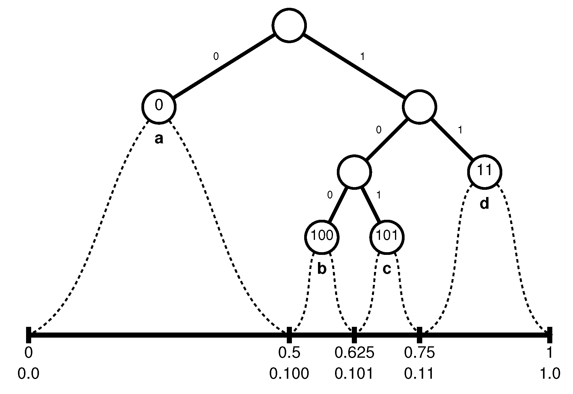
The following example will clarify this claim. Consider the alphabet $A=\left\{\mathsf{a},\mathsf{b},\mathsf{c},\mathsf{d}\right\}$ with dyadic probabilities $P=\{\frac{1}{2},\frac{1}{8},\frac{1}{8},\frac{1}{4}\}$, respectively, and suppose the partition of the interval $I_0$ is in this given order, that is, the boundaries of the subintervals are 0, $\frac{1}{2}$, 0.625, 0.75 and 1, or 0, 0.1, 0.101, 0.11 and 1 in the standard binary representation.

• If the first letter to be encoded is a, the interval will be narrowed to $I_1=[0,\frac{1}{2})$, and whatever the final interval will be, we know already that it is included in $I_1$, so that the first bit of the encoding string must be a zero.
• If the first letter of the input is b, the interval $I_0$ will be narrowed to $I_1=[0.1,0.101)$ (in binary); any real number in $I_1$ that can be identified as belonging only to $I_1$ must start with $0.100\cdots$, which contributes the bits 100 to the output file. Note that 0.1 or 0.10 also belong to $I_1$, but there are also numbers in other subintervals starting with 0.1 or 0.10, so that the shortest representation of $\frac{1}{2}$ that can be used unambiguously to further sub-partition the interval is 0.100.
• Similarly, if the first letter to be encoded is c, $I_0$ will be narrowed to $I_1=[0.101,0.11)$, which contributes the bits 101 to the output file, and for the last case,
• if the first letter is d, the new interval will be $I_1=[0.11,1)$, contributing the bits 11.

Summarizing these cases, we know already, after having processed a single character, that the first bits of the output must be 0, 100, 101 or 11, according to whether the first character is a, b, c or d, respectively. In any case, arithmetic coding then rescales the interval and restarts as if it were $[0,1)$ again, which means that also the second, and subsequent, character(s) will contribute 0, 100, 101 or 11, according to whether they are a, b, c or d. But $\{0,100,101,11\}$ is one of the possible Huffman codes for the given probability distribution, so that in this case, both algorithms generate bit sequences that are not only of the same length, but they produce exactly the same output. This connection is visualized in Figure 1. For example, if one wishes to encode the string bcbad, the output could be the number 0.586669921875 = 0.100101100011, just as if the above Huffman code had been used, which yields 100-101-100-0-11.

This example can be generalized to any dyadic distribution, as formulated in the following lemma.

Lemma 1.

If the elements of an alphabet $A=\{a_1,\dots ,a_n\}$ in a text T occur with a dyadic probability distribution $p_1,\dots ,p_n$, then it is possible to partition the interval $[0,1)$ in such a way that an arithmetic encoding of T produces a compressed file which is identical to one of the possible binary encodings using a Huffman code.

Proof. 

The proof is by induction on the size n of the alphabet A, and inspired by the proof of the optimality of Huffman coding [34]. For $n=2$, there is only one possible dyadic distribution, with $p_1=p_2=\frac{1}{2}$, and a Huffman code assigns the codewords 0 and 1 to the elements $a_1$ and $a_2$ (or vice versa), respectively. The corresponding partition of the interval $[0,1)$ is into $[0,\frac{1}{2})$ and $[\frac{1}{2},1)$. If the following character is $a_1$ (resp., $a_2$), the current interval used in arithmetic coding is narrowed to its left (resp., right) half, so that the following bit has to be 0 (resp., 1), which is identical to the following bit generated by the Huffman code.

Assume now the truth of the lemma for $n-1$ and consider an alphabet $A=\{a_1,\dots ,a_n\}$ of size n. Without loss of generality, let $a_n$ be a character with smallest probability $p_n=2^{-\ell }$. There must be at least one more character having the same probability $2^{-\ell }$, otherwise the probabilities can not possibly sum up to 1; this is because only $p_n$ would then have a 1-bit in the ℓ-th position to the right of the binary point of its binary representation. Again without loss of generality, one other character with probability $2^{-\ell }$ could be $a_{n-1}$.

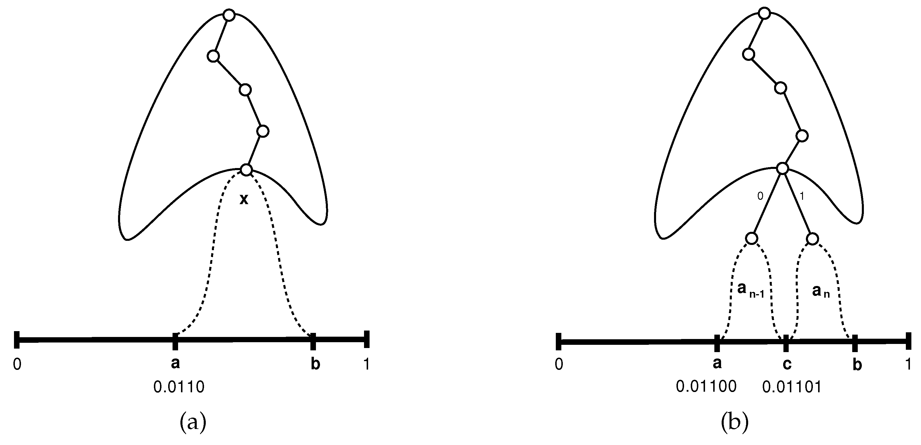
Consider now the alphabet $A^{\prime }=\{a_1,\dots ,a_{n-2},x\}$, obtained from A by eliminating the characters $a_{n-1}$ and $a_n$, and by adjoining a new character x to which we assign the probability $2^{-\ell }+2^{-\ell }=2^{-\ell +1}$. The alphabet $A^{\prime }$ is of size $n-1$ and its elements have a dyadic distribution, so we may apply the inductive hypothesis. In particular, there is a partition of $[0,1)$ in which the sub-interval corresponding to the character x is $[a,b)$, and such that the $\ell -1$ first bits to the right of the binary point of the binary representation of a form the codeword assigned by the Huffman code to the character x. Denote this string of $\ell -1$ bits by $\alpha$. Figure 2a schematically depicts this situation: the branch of the Huffman tree leading to the leaf corresponding to x is shown, as well as the associated interval $[a,b)$. In this particular case, $\ell =5$, $a=0.375$, and the 4 first bits after the binary point of ${0.375}_{10}=0.01100{\cdots }_2$ are the Huffman codeword $\alpha =0110$ of x.

Let us now return to the alphabet A of size n. We leave the partition of $[0,1)$ as for the alphabet $A^{\prime }$, except that the sub-interval $[a,b)$ will be split into halves $[a,c)$ and $[c,b)$, where $c=\frac{a+b}{2}$, each of size $2^{-\ell }$, and corresponding, respectively, to the characters $a_{n-1}$ and $a_n$. This is schematically shown in Figure 2b.

• If the current character y to be processed is one of $a_1,\dots ,a_{n-2}$, it follows from the inductive assumption that arithmetic coding will narrow the current interval so that the following bits of the output stream are equal to the Huffman codeword of y.
• If the current character is $a_{n-1}$, the corresponding interval is $[a,c)$. From the inductive assumption we know that if we would deal with $A^{\prime }$ and the following character would be x, the next generated bits would have been $\alpha$, so if we now restrict our attention to $[a,c)$, the left half of $[a,b)$, the next generated bits have to be $\alpha 0$. But $\alpha 0$ is exactly the Huffman codeword of $a_{n-1}$ in A.
• Similarly, if the next character is $a_n$, the restriction would be to $[c,b)$ and the next generated bits would have to be $\alpha 1$, which is the Huffman codeword of $a_n$ in A.

Summarizing, we have found a partition of $[0,1)$ for which arithmetic coding produces identical output to one of the possible Huffman codes, also for any dyadic alphabet of size n, which concludes the proof.  □

The randomness of the output of arithmetic coding thus follows from that of Huffman coding with the same assumptions.

Theorem 1.

If the elements in a text occur with a dyadic probability distribution and independently of each other, then applying some arithmetic coder will produce output that seems random, in the sense that every possible substring of length m will occur with probability $2^{-m}$.

Proof. 

From the lemma we know that in the case of a dyadic distribution, Huffman and arithmetic coding may produce the same binary string B as output. If, in addition, the occurrences of the elements are independent of each other, this string B will be random in the above sense according to the theorem in Section 2.3 of Reference [30].  □

There are also dynamic variants of Huffman and arithmetic coding, in which the i-th element is encoded on the basis of a Huffman code or a partition of the initial interval corresponding to the $i-1$ preceding elements. An efficient algorithm avoiding the repeated construction of the Huffman tree can be found in Reference [35]; for dynamic arithmetic coding, the partition of the interval is simply updated after the processing of each element. Adaptive methods may improve the compression, especially on heterogeneous files, but there are other inputs for which the static variants are preferable.

As to randomness of dynamically Huffman encoded texts, the fact that an element is not always represented by the same codeword seems to be advantageous, but in fact, at least for independently appearing elements with dyadic probability distributions, there should be no difference: we know that each time the interval is rescaled in arithmetic coding, or at the end of the processing of a codeword in Huffman coding, each of the following characters will contribute the binary string $s_i$ to the output file, according to whether the next element is $a_i$, where $s_i$ is the codeword corresponding to $a_i$ in the given Huffman code. The only difference between static and dynamic coding is that the Huffman tree, and the partition of the interval $[0,1)$, may change, but as long as dyadicity and independence are maintained, the above arguments apply here as well.

2.3. LZW

We have dealt so far with statistical compression and turn now to another family of methods based on dictionaries. The most famous representatives of this family are the algorithms due to Ziv and Lempel and their variants. Dictionary methods compress by replacing substrings of the input text by (shorter) pointers to a dictionary, in which a collection of appropriate substrings has been stored. In LZW [36,37,38], the dictionary D is initialized as containing the single characters alone, and then adaptively updated by adding any newly encountered substring in the parsing process that has not been adjoined previously to D. The text is parsed sequentially into a sequence of elements of the currently constructed dictionary D, where at each stage, the longest possible element of D is chosen.

The output of this compression method is a sequence of pointers to the dictionary D, and the randomness of the compressed file will thus depend on the way chosen to encode these pointers. In its original implementation, LZW is designed to work with alphabets of up to 256 characters and we shall stick, for simplicity, to this restriction, which could easily be extended. LZW starts with a dictionary of size 512 which stores already all the single characters in ascii and is therefore half filled. Any pointer to D is just the 9-bit binary representation of the index of the addressed entry. After having processed 256 elements of the input file, thereby adding 256 entries to D, the dictionary is filled up and its size is doubled to 1024 entries. From this point on, all the pointers to D are encoded as 10-bit integers. In general, after processing $2^9,2^{10},\dots ,2^i,\dots$ more elements of the input file, the size of the dictionary is doubled to $2^{11},2^{12},\dots ,2^{i+2},\dots$ entries, up to a predetermined maximal size, say $2^{18}$. There are several options to continue, like restarting from scratch with 9 bits, or considering the dictionary as static and not adjoining any more strings.

The following argument claims that an LZW-encoded file will generally not be random. At any stage of the algorithm, the ratio between the number of occupied entries and the current size of D is between $\frac{1}{2}$ and 1. This suggests that the probability for a referenced string to fall into the lower half of the dictionary is higher than for the upper part. But all indices of the lower part entries have a 0 in their leftmost bits, and those of the upper part start with 1. We conclude that the probability for the leftmost bits of every codeword, which are very specific bits in the compressed file, those at bit positions

$$\begin{array}{c}0,9,18,\dots ,\hfill \\ 9\times 256,9\times 256+10,9\times 256+20,\dots ,\hfill \\ 9\times 256+10\times 512,9\times 256+10\times 512+11,9\times 256+10\times 512+22,\dots \hfill \end{array}$$

to be equal to 0 is higher than to be equal to 1, contradicting randomness.

The following variant of LZW tries to rectify this shortcoming. Since we suspect the distribution of the possible values of the first bit of every pointer to the dictionary to be biased, and since we know exactly where to locate these bits in the compressed file (every 9-th bit, then every 10-th, etc.), we may split each pointer and aggregate the output in two separate strings: F for the first bit of each index, and T concatenating the tails of the numbers, that is, their values after having stripped the leading bit of each. If the distribution in F is not uniform, a simple arithmetic coder, even on the individual bits, can only improve the compression. Indeed, the contribution of each encoded bit of T will then be the entropy $H\left(p\right)$, where p is the probability of a 1-bit, and as mentioned earlier, if $p\ne \frac{1}{2}$, then $H\left(p\right)<1$, so that the encoding of F will be strictly shorter than $\left|F\right|$.

The new variant will thus improve the compression on the one hand, but also the randomness, since we replace a part of the compressed file, which we know is not uniformly distributed, by its arithmetic encoding, which has been dealt with above and has been reported to produce seemingly random output in empirical tests [23]. A similar approach, using different encodings, is used in gzip, which first encodes a file using LZ77 [37] producing characters and $(offset,length)$ pairs, and then encodes the offsets by means of a certain Huffman tree, and the characters and lengths by means of another.

3. Empirical Tests

The following series of tests to check the randomness of compressed data has been performed. The test files were from different languages and with different alphabets, and they all yielded essentially the same behavior. To allow a fair comparison, we present here only the results on one of the files, the King James version of the English Bible (The file can be accessed at http://u.cs.biu.ac.il/~tomi/files/ebib2), in which the text was stripped of all punctuation signs, leaving only upper and lower case characters and blank. There is no claim that the file is representative of “typical” input, so the results should be interpreted as an illustration of the above ideas, rather than as empirical evidence.

To check whether the compressed sequence is m-distributed, we collected statistics on the frequencies of all (overlapping) bit-strings of length m, for $m=1,\dots ,8$. For each m, the distribution of the $2^m$ possible m-bit patterns was compared to the expected uniform distribution for a perfectly random sequence. We used two different measures to quantify the distance between the obtained and expected distributions, and considered that the smaller the obtained distance values, the better the randomness.

• A measure for the spread of values could be the standard deviation $\sigma$, which is generally of the order of magnitude of the average $\mu$, so their ratio $\frac{\sigma }{\mu }$ may serve as a measure of the skewness of the distribution.
• Given two probability distributions $P=\{p_1,\dots ,p_n\}$ and $Q=\{q_1,\dots ,q_n\}$, the Kullback–Leibler (KL) divergence [39], defined as

  $$D_{KL}(P\parallel Q)=\sum _{i=1}^n{p}_{i}log\frac{p_i}{q_i},$$

  gives a one-sided, asymmetric, distance from P to Q, which vanishes for $P=Q$.

In the special case treated here, the second distribution Q is uniform on $2^m$ elements, $U_m=\{2^{-m},\dots ,2^{-m}\}$, thus

$$D_{KL}(P\parallel U_m)=\sum _{i=1}^{2^m}{p}_{i}log\left(2^m{p}_i\right)=\sum _{i=1}^{2^m}{p}_{i}log{p}_i+m\sum _{i=1}^{2^m}{p}_i=m-H\left(P\right),$$

where $H\left(P\right)$ is the entropy of P.

Table 1. Ratio $\frac{\sigma }{\mu }$ of standard deviation to average within the set of $2^m$ values for $m=1,\dots ,8$.

alg $\setminus$ $\mathit{m}$	1	2	3	4	5	6	7	8	$\frac{{\mathit{avg}}_{\mathbf{alg}}}{{\mathit{avg}}_{\mathbf{random}}}$	compr
arith	0.00004	0.0001	0.0007	0.0011	0.0017	0.0025	0.0036	0.0050	0.3	52.4
random	0.0015	0.0021	0.0029	0.0040	0.0054	0.0078	0.0108	0.0149	1	–
gzip	0.0072	0.0129	0.0168	0.0204	0.0234	0.0263	0.0290	0.0318	3.4	31.2
newlzw	0.0174	0.0251	0.0314	0.0367	0.0415	0.0459	0.0501	0.0541	6.1	30.2
oldlzw	0.0237	0.0341	0.0427	0.0504	0.0572	0.0633	0.0691	0.0746	8.4	30.3
bwt	0.0204	0.0326	0.0415	0.0544	0.0674	0.0825	0.1025	0.1236	10.6	23.3
hufwrd	0.0420	0.0595	0.0730	0.0851	0.0976	0.1130	0.1299	0.1500	15.2	21.7
hufcar	0.0834	0.1240	0.1609	0.2018	0.2661	0.3533	0.4488	0.5695	44.7	52.8
ascii	0.1227	0.1736	0.2506	0.3234	0.4457	0.5721	0.8007	1.1124	76.9	100

and

Table 2. Kullback—Leibler distance from uniform distribution.

alg $\setminus$ $\mathit{m}$	1	2	3	4	5	6	7	8	$\frac{{\mathit{avg}}_{\mathbf{alg}}}{{\mathit{avg}}_{\mathbf{random}}}$
arith	0.000000001	0.000000003	0.00000010	0.00000021	0.00000042	0.00000076	0.00000135	0.00000224	0.02
random	0.00000154	0.00000308	0.00000625	0.00001152	0.00002079	0.00004397	0.00008407	0.00015928	1
gzip	0.00004	0.0001	0.0001	0.0001	0.0001	0.0001	0.0001	0.0001	2
newlzw	0.0002	0.0002	0.0002	0.0002	0.0002	0.0002	0.0003	0.0003	6
oldlzw	0.0004	0.0004	0.0004	0.0004	0.0005	0.0005	0.0005	0.0005	11
bwt	0.0003	0.0004	0.0004	0.0005	0.0007	0.0008	0.0011	0.0014	17
hufwrd	0.0013	0.0013	0.0013	0.0013	0.0014	0.0015	0.0017	0.0020	36
hufcar	0.0050	0.0058	0.0069	0.0087	0.0122	0.0173	0.0223	0.0289	324
ascii	0.0109	0.0109	0.0170	0.0228	0.0338	0.0452	0.0699	0.1014	944

display the values of the measures $\frac{\sigma }{\mu }$ and $\frac{1}{m}{D}_{KL}(P\parallel U_m)$ (KL is normalized), respectively, for the following set of files, all encoding the same Bible file mentioned above, except for file random.

Random—a sequence of $2^{20}$ randomly and independently chosen bits has been generated, to serve as a baseline for a perfectly random file. Ideally, all probabilities should be $2^{-m}$, but there are of course fluctuations, and our measures try to quantify them.

Arith—compressed file using static arithmetic coding.

Gzip—compressed file using gzip, a Ziv-Lempel variant on which Huffman coding is superimposed.

Newlzw—compressed file using the variant of LZW encoding the leading and the other bits of each dictionary entry index separately.

Oldlzw—compressed file using the original LZW.

Bwt—compressed file using bzip2 based on the Burrows–Wheeler transform [40].

Hufwrd—compressed file using Huffman coding on the 611,793 words (11,377 different words) of the Bible.

Hufcar—compressed file using Huffman coding on the 52 different characters in the Bible file.

Ascii—is the uncompressed input file itself, of size 3,099,227 bytes.

The standard variants of the Unix operating system for gzip and bzip2, without parameters, have been used; the implementation of arithmetic coding is from Nelson’s book [41], and those of the variants of LZW and Huffman coding have been written by the authors. The lines in the tables are arranged in increasing order of the average values in each row. One can see that all the values, for both measures, are very small, especially when compared to those in the last line corresponding to the original, uncompressed file. As expected, the values for the random file, were by far the smallest, for the KL divergence even by orders of magnitude, except for the values obtained for arithmetic coding, which seem to be “more random than random”. This shows that the random number generator of the awk program we used to produce the random file needs apparently to be improved. Both measures yield the same order of the compression methods.

Table 1 shows also, in its last column, the compression ratio defined as the size of the compressed as a percentage of the original file. We define $av{g}_{\mathsf{alg}}$ to be the average of the values in columns headed 1 to 8 for the line corresponding to compression method alg. In both tables, the columns headed $\frac{av{g}_{\mathsf{alg}}}{av{g}_{\mathsf{random}}}$ give this ratio, showing that the standard deviations can be between 3 to 77 times larger than for the random benchmark. The KL divergence is 2 to 300 times larger for compression methods, and almost 1000 times for an uncompressed file.

We see that good compression is not necessarily correlated with randomness: the smallest file (about 22%) was obtained by Huffman encoding the text as a sequence of words, whereas its randomness is 15 or 36 times worse than for random. The new variant of LZW improves the compression performance only by about 0.4% relative to the standard LZW version, but improves the randomness by 28% for the average $\frac{\sigma }{\mu }$ and by 45% for the average KL distance.

4. Conclusions

We have examined the randomness of compressed data and shown that while the uniformity of the probability distributions of the occurrences of all possible bit patterns may be better than for uncompressed files, there are still quite large differences between the compression methods themselves, suggesting that cascading compression techniques might sometimes be useful. Surprisingly, the best compression schemes (hufwrd and bwt) do not have the most random output, suggesting that these schemes can be further improved. Moffat [42] considers a more involved model, first and second order word-based compressions, and analyzes the space savings by combining them with arithmetic, Huffman, and move-to-front methods. Using a higher order Markov model [43] may also increase randomness.

We had no intention to cover all possible lossless compression techniques in this work, and concentrated only on a few selected ones. Some other interesting ones, such as PPM [4] and CTW [44] have been left for future work. Another line of investigation deals with compression methods that are not for general purpose, but custom tailored for files with known structure, such as dictionaries, concordances, lists, B-trees and bitmaps, as can be found in large full-text information retrieval systems.

References

- Huffman, D.A. A Method for the Construction of Minimum-Redundancy Codes. Available online: http://compression.ru/download/articles/huff/huffman_1952_minimum-redundancy-codes.pdf (accessed on 5 April 2020).
- Elias, P. Universal codeword sets and representations of the integers. IEEE Trans. Inf. Theory 1975, 21, 194–203. [Google Scholar] [CrossRef]
- Vitter, J.S. Algorithm 673: Dynamic Huffman coding. ACM Trans. Math. Softw. 1989, 15, 158–167. [Google Scholar] [CrossRef]
- Cleary, J.; Witten, I. Data Compression Using Adaptive Coding and Partial String Matching. IEEE Trans. Commun. 1984, 32, 396–402. [Google Scholar] [CrossRef] [Green Version]
- Storer, J.A.; Szymanski, T.G. Data compression via textural substitution. J. ACM 1982, 29, 928–951. [Google Scholar] [CrossRef]
- Klein, S.T.; Shapira, D. Context Sensitive Rewriting Codes for Flash Memory. Comput. J. 2019, 62, 20–29. [Google Scholar] [CrossRef]
- Klein, S.T.; Shapira, D. On improving Tunstall codes. Inf. Process. Manag. 2011, 47, 777–785. [Google Scholar] [CrossRef] [Green Version]
- Amir, A.; Benson, G. Efficient two-dimensional compressed matching. In Proceedings of the Data Compression Conference, Snowbird, UT, USA, 24–27 March 1992; pp. 279–288. [Google Scholar]
- Shapira, D.; Daptardar, A.H. Adapting the Knuth-Morris-Pratt algorithm for pattern matching in Huffman encoded texts. Inf. Process. Manag. 2006, 42, 429–439. [Google Scholar] [CrossRef] [Green Version]
- Klein, S.T.; Shapira, D. Compressed Pattern Matching in jpeg Images. Int. J. Found. Comput. Sci. 2006, 17, 1297–1306. [Google Scholar] [CrossRef]
- Klein, S.T.; Shapira, D. Compressed matching for feature vectors. Theor. Comput. Sci. 2016, 638, 52–62. [Google Scholar] [CrossRef]
- Klein, S.T.; Shapira, D. Compressed Matching in Dictionaries. Algorithms 2011, 4, 61–74. [Google Scholar] [CrossRef]
- Baruch, G.; Klein, S.T.; Shapira, D. Applying Compression to Hierarchical Clustering. In Proceedings of the SISAP 2018: 11th International Conference on Similarity Search and Applications, Lima, Peru, 7–9 October 2018; pp. 151–162. [Google Scholar]
- Jacobson, G. Space efficient static trees and graphs. In Proceedings of the 30th Annual Symposium on Foundations of Computer Science, Research Triangle Park, NC, USA, 30 October–1 November 1989; pp. 549–554. [Google Scholar]
- Navarro, G. Compact Data Structures: A Practical Approach; Cambridge University Press: Cambridge, UK, 2016. [Google Scholar]
- Klein, S.T.; Shapira, D. Random access to Fibonacci encoded files. Discret. Appl. Math. 2016, 212, 115–128. [Google Scholar] [CrossRef]
- Baruch, G.; Klein, S.T.; Shapira, D. A space efficient direct access data structure. J. Discret. Algorithms 2017, 43, 26–37. [Google Scholar] [CrossRef]
- Fariña, A.; Navarro, G.; Paramá, J.R. Boosting Text Compression with Word-Based Statistical Encoding. Comput. J. 2012, 55, 111–131. [Google Scholar] [CrossRef] [Green Version]
- Manber, U.; Myers, G. Suffix Arrays: A New Method for On-Line String Searches. SIAM J. Comput. 1993, 22, 935–948. [Google Scholar] [CrossRef]
- Huo, H.; Sun, Z.; Li, S.; Vitter, J.S.; Wang, X.; Yu, Q.; Huan, J. CS2A: A Compressed Suffix Array-Based Method for Short Read Alignment. In Proceedings of the 2016 Data Compression Conference (DCC), Snowbird, SLC, USA, 30 March–1 April 1 2016; pp. 271–278. [Google Scholar]
- Benza, E.; Klein, S.T.; Shapira, D. Smaller Compressed Suffix Arrays. Comput. J. 2020, 63. [Google Scholar] [CrossRef] [Green Version]
- Rubin, F. Cryptographic Aspects of Data Compression Codes. Cryptologia 1979, 3, 202–205. [Google Scholar] [CrossRef]
- Klein, S.T.; Shapira, D. Integrated Encryption in Dynamic Arithmetic Compression. In Proceedings of the 11th International Conference on Language and Automata Theory and Applications, Umeå, Sweden, 6–9 March 2017; pp. 143–154. [Google Scholar]
- Gillman, D.W.; Mohtashemi, M.; Rivest, R.L. On breaking a Huffman code. IEEE Trans. Inf. Theory 1996, 42, 972–976. [Google Scholar] [CrossRef] [Green Version]
- Fraenkel, A.S.; Klein, S.T. Complexity Aspects of Guessing Prefix Codes. Algorithmica 1994, 12, 409–419. [Google Scholar] [CrossRef]
- L’Ecuyer, P.; Simard, R.J. TestU01: A C library for empirical testing of random number generators. ACM Trans. Math. Softw. 2007, 33, 22:1–22:40. [Google Scholar] [CrossRef]
- Chang, W.; Yun, X.; Li, N.; Bao, X. Investigating Randomness of the LZSS Compression Algorithm. In Proceedings of the 2012 International Conference on Computer Science and Service System, Nanjing, China, 11–13 August 2012. [Google Scholar]
- Chang, W.; Fang, B.; Yun, X.; Wang, S.; Yu, X. Randomness Testing of Compressed Data. arXiv 2010, arXiv:1001.3485. [Google Scholar]
- Knuth, D.E. The Art of Computer Programming, Volume II: Seminumerical Algorithms; Addison-Wesley: Reading, MA, USA, 1969. [Google Scholar]
- Klein, S.T.; Bookstein, A.; Deerwester, S.C. Storing Text Retrieval Systems on CD-ROM: Compression and Encryption Considerations. ACM Trans. Inf. Syst. 1989, 7, 230–245. [Google Scholar] [CrossRef]
- Longo, G.; Galasso, G. An application of informational divergence to Huffman codes. IEEE Trans. Inf. Theory 1982, 28, 36–42. [Google Scholar] [CrossRef]
- Bookstein, A.; Klein, S.T. Is Huffman coding dead? Computing 1993, 50, 279–296. [Google Scholar] [CrossRef]
- Witten, I.H.; Neal, R.M.; Cleary, J.G. Arithmetic Coding for Data Compression. Commun. ACM 1987, 30, 520–540. [Google Scholar] [CrossRef]
- Klein, S.T. Basic Concepts in Data Structures; Cambridge University Press: Cambridge, UK, 2016. [Google Scholar]
- Vitter, J.S. Design and analysis of dynamic Huffman codes. J. ACM 1987, 34, 825–845. [Google Scholar] [CrossRef]
- Welch, T.A. A Technique for High-Performance Data Compression. IEEE Comput. 1984, 17, 8–19. [Google Scholar] [CrossRef]
- Ziv, J.; Lempel, A. A universal algorithm for sequential data compression. IEEE Trans. Inf. Theory 1977, 23, 337–343. [Google Scholar] [CrossRef] [Green Version]
- Ziv, J.; Lempel, A. Compression of individual sequences via variable-rate coding. IEEE Trans. Inf. Theory 1978, 24, 530–536. [Google Scholar] [CrossRef] [Green Version]
- Kullback, S.; Leibler, R.A. On information and sufficiency. Ann. Math. Stat. 1951, 22, 79–86. [Google Scholar] [CrossRef]
- Burrows, M.; Wheeler, D.J. A Block Sorting Lossless Data Compression Algorithm. Available online: https://www.hpl.hp.com/techreports/Compaq-DEC/SRC-RR-124.pdf (accessed on 5 April 2020).
- Nelson, M.; Gailly, J.L. The Data Compression Book, 2nd ed.; M & T Books: New York, NY, USA, 1996. [Google Scholar]
- Moffat, A. Word-based Text Compression. Softw. Pract. Exp. 1989, 19, 185–198. [Google Scholar] [CrossRef]
- Cormack, G.V.; Horspool, R.N. Data Compression Using Dynamic Markov Modelling. Comput. J. 1987, 30, 541–550. [Google Scholar] [CrossRef]
- Willems, F.M.J.; Shtarkov, Y.M.; Tjalkens, T.J. The context-tree weighting method: basic properties. IEEE Trans. Inf. Theory 1995, 41, 653–664. [Google Scholar] [CrossRef] [Green Version]
Figure 1.
Connection between Huffman and arithmetic coding on dyadic probabilities.
Figure 2.
Schematic view of the inductive step of the proof.