Article

Benchmarking Machine Learning Models to Assist in the Prognosis of Tuberculosis

by
Maicon Herverton Lino Ferreira da Silva Barros
1,
Geovanne Oliveira Alves
1,
Lubnnia Morais Florêncio Souza
1,
Elisson da Silva Rocha
1,
João Fausto Lorenzato de Oliveira
1,
Theo Lynn
2,
Vanderson Sampaio
3 and
Patricia Takako Endo
1,*
1
Programa de Pós-Graduação em Engenharia de Computação (PPGEC), Universidade de Pernambuco, Recife 50720-001, Pernambuco, Brazil
2
Business School, Dublin City University, Dublin 9, Dublin, Ireland
3
Fundação de Medicina Tropical Doutor Heitor Vieira Dourado, Manaus 69040-000, Amazonas, Brazil
*
Author to whom correspondence should be addressed.
Informatics 2021, 8(2), 27; https://doi.org/10.3390/informatics8020027
Submission received: 8 March 2021 / Revised: 8 April 2021 / Accepted: 9 April 2021 / Published: 15 April 2021
(This article belongs to the Special Issue Machine Learning in Healthcare)

Abstract

:
Tuberculosis (TB) is an airborne infectious disease caused by organisms in the Mycobacterium tuberculosis (Mtb) complex. In many low and middle-income countries, TB remains a major cause of morbidity and mortality. Once a patient has been diagnosed with TB, it is critical that healthcare workers make the most appropriate treatment decision given the individual conditions of the patient and the likely course of the disease based on medical experience. Depending on the prognosis, delayed or inappropriate treatment can result in unsatisfactory results including the exacerbation of clinical symptoms, poor quality of life, and increased risk of death. This work benchmarks machine learning models to aid TB prognosis using a Brazilian health database of confirmed cases and deaths related to TB in the State of Amazonas. The goal is to predict the probability of death by TB thus aiding the prognosis of TB and associated treatment decision making process. In its original form, the data set comprised 36,228 records and 130 fields but suffered from missing, incomplete, or incorrect data. Following data cleaning and preprocessing, a revised data set was generated comprising 24,015 records and 38 fields, including 22,876 reported cured TB patients and 1139 deaths by TB. To explore how the data imbalance impacts model performance, two controlled experiments were designed using (1) imbalanced and (2) balanced data sets. The best result is achieved by the Gradient Boosting (GB) model using the balanced data set to predict TB-mortality, and the ensemble model composed by the Random Forest (RF), GB and Multi-Layer Perceptron (MLP) models is the best model to predict the cure class.

1. Introduction

Tuberculosis (TB) is an airborne infectious disease caused by organisms in the Mycobacterium tuberculosis complex (Mtb). In many low-income and middle-income countries, such as South Africa, Nigeria and India, TB continues to be a major cause of morbidity and mortality [1,2]. Despite World Health Organization (WHO) efforts to reduce the incidence of TB and its mortality rate, 10 million people fell ill with TB and 1.2 million deaths were registered in 2019 worldwide [2]. According to the WHO Global Tuberculosis Report 2020 [2], in the Americas, “TB incidence is slowly increasing, owing to an upward trend in Brazil”. In the same year, Brazil registered 96 thousand cases of TB with a mortality rate of 7% [3]; Brazil has one of the highest TB rates in the world [4]. According to Ranzani et al. [5], TB is a marker of social inequity and the paradigm of poverty-related diseases. After a period of poverty reduction, poverty rates began to grow again in Latin America in 2015 primarily driven by increases in vulnerable communities in Brazil and Venezuela, and specifically increased homelessness and incarceration [5].
The Brazilian Sistema Único de Saúde (SUS) is one of the largest public health systems in the world. It is responsible for providing primary care services, of varying complexity, including blood donation, chemotherapy, organ transplantation, amongst others [6]. SUS also provides free vaccines and medicines for people with diabetes, arterial hypertension, HIV, Alzheimer’s etc. In addition, SUS is responsible for emergency response through the Serviço de Atendimento Móvel de Urgência (SAMU) [7]. Currently, more than three-fourths of the Brazilian population rely exclusively on SUS health services for medical treatment [8]. The Sistema de Informação de Agravos de Notificação (SINAN) is an SUS system mainly comprising notifications of diseases on the National Compulsory Notification List of diseases. These data are routinely generated by the Epidemiological Surveillance System. SINAN has a database with demographic, clinical and laboratory data on TB patients, the SINAN-TB, that can potentially be used for TB prognosis.
Prognosis research is the study of relationships between incidences of outcomes and predictors in defined populations of people with a disease, in this case, TB [9]. While diagnosis is the identification of an illness by examination of the symptoms, prognosis is concerned causes of disease progression, prediction of risk in individuals, and individual response to treatment so that the improved opportunities for mitigating disease progression are leveraged, and the risk adverse outcomes reduced [10]. Therefore, once a diagnosis is made, it is necessary to understand the severity of the clinical situation in order to make decisions about the most appropriate treatment, including hospitalisation or admission to an Intensive Care Unit (ICU). The analysis of severity is essential for more reliable communication of outcome risk to patients, improving opportunities to mitigate disease progression, to improve the quality of life of patients, and to effectively manage health resources. Unfortunately, the quality of much prognosis research is poor [10].
The main focus of our work is to evaluate machine learning models to aid TB prognosis and associated decision making by predicting the probability of death using patient demographic, clinical and laboratory data. Comparisons with extant research is complicated by the difference in goals and data used. Consequently, we benchmark nine machine learning models used in extant machine learning studies related to TB detection—Logistic Regression (LR), Linear Discriminant Analysis (LDA), K-Nearest Neighbor (KNN), Naive Bayes (NB), Decision Trees (DT), Support Vector Machine (SVM), Gradient Boosting (GB), Random Forest (RF) and Multi-Layer Perceptron (MLP). Our benchmarking methodology focuses on disease prognosis, not detection, and is designed to (a) identify the most relevant fields using feature selection techniques; (b) apply a randomized search technique to select the optimal hyperparameters of the machine learning models; and (c) propose an ensemble model [11,12,13] that combines two or more machine learning models in order to achieve better results and reduce the risk associated with using a sub-optimal or inappropriate models.

2. Related Works

The search for early diagnosis of TB is a goal of health programs around the world due to the inherent difficulties in eliminating TB [14]. To date, extant research has primarily explored the use of deep learning for the diagnosis of TB from radiography [15,16,17] or microscopic images [18,19]. A number of studies have also explored the use of deep learning to predict mortality and co-morbidities [20,21,22]. These studies focus on the diagnosis of TB. There is, however, a dearth of studies on prognosis of TB, the focus of this work.
Recently, Peetluk et al. [23] published the first systematic review regarding models proposed to predict TB treatment outcomes. They followed the WHO definition of treatment outcomes for patients with TB i.e., treatment completion, cure, treatment success, treatment failure, death, loss to follow-up, and not evaluated. 37 prediction models were identified, 16 of which examined death as an outcome [24,25,26,27,28,29,30,31,32,33,34,35,36,37,38]. None of the 16 cited papers that examined death as an outcome used machine learning; 11 used LR. It is important to note that Peetluk et al. [23] do not classify LR as machine learning in their review as the LR analysis was used as a statistical methodology to understand the relationship between attributes and their prevalence. In the few machine learning studies identified, it was used primarily for predicting treatment completion [39] or unfavourable outcomes [40,41].
Hussain and Junejo [39] propose and evaluate three machine learning models-SVM, RF and Neural Network (NN). Their data set comprised 4213 records from an unidentified location; 64.37% of the records represented completed treatments. The outcome predicted by the models is treatment completion and the following metrics were used to compare the models—accuracy, precision, sensitivity, and specificity. The RF model achieved the highest accuracy (76.32%); the SVM outperformed all models in precision (73.05%) and specificity (95.71%). The NN achieved the highest sensitivity (68.5%).
Killian et al. [40] used an Indian data set comprising 16,975 patient records to classify unfavorable outcomes. They considered death, treatment failure, loss to follow-up and not evaluated as the same class. They proposed a deep learning model, named LSTM Real-time Adherence Predictor (LEAP) and compared it against a RF model. LEAP achieved an AUROC of 0.743 and the RF, 0.722.
Sauer et al. [41] also compared different machine learning models to classify unfavorable outcomes. They used a multi-country data set (Azerbaijan, Belarus, Georgia, Moldova and Romania) composed of 587 records of TB cases. They evaluated three machine learning models, RF, and SVM with linear kernel and polynomial kernel, against classic regression approaches, stepwise forward selection, stepwise backward elimination, backward elimination and forward selection, and Least Absolute Shrinkage and Selection Operator (LASSO) regression. Sauer et al. [41] do not present the outcome number of the models thus negatively impacting comparability. Furthermore, their models presented very low sensitivity scores (SVM with linear kernel achieved 21%) and high specificity scores (SVM with linear kernel achieved 94%), suggesting that their model has underfitting/overfitting issues.
While it did not feature in Peetluk et al.’s systematic review [23], Kalhori et al. [42] explored the use of machine learning to predict the outcome of a course of TB treatment. Using a data set of 6450 TB incidence from Iran in 2005, they compared six classifiers including DT, Bayesian networks, LR, MLP, Radial Basis Function, and SVM. The DT model presented the best performance with 97% of Area Under The Curve (AUC) Receiver Operating Characteristics (ROC).
In contrast to the limited published research on the topic of TB prognosis using machine learning, we use computational techniques to (i) reduce the dimensionality of the data set, and (ii) find optimal hyperparameter configuration. Furthermore, and critically, we also evaluate ensemble models. Our study uses an extensive data set from Brazil, a country with one of the highest incidences of TB in the world. In this way, we advance the state of the art in the study of machine learning for TB prognosis.

3. Background

3.1. Feature Selection Techniques

The feature selection techniques are algorithms that can be used to select a subset of fields from the original database [43]. In this work, we compare the performance of four different feature selection techniques: Sequential Forward Selection (SFS), Sequential Forward Floating Selection (SFFS), Sequential Backward Selection (SBS), Sequential Backward Floating Selection (SBFS). The stop criteria for all techniques is 17 fields as per [44] and the feature selection is based on the F1-score.
The SFS is a greedy search algorithm that selects the feature set following a bottom-up search procedure. The algorithm starts from an empty set and fills this set iteratively [45]. It is widely used because it is simple and fast [46]. SFFS is an extension of the SFS algorithm that includes a new feature using the SFS procedure followed by successive conditional exclusion of the least significant feature in the set of features. The final feature set is the one that provides a subset of the best features [47].
The SBS starts with the complete set of features, and it iteratively removes the less significant features, until some closure criterion is met [48]. SBFS is an extension of the SBS technique and it removes irrelevant features by selecting a subset of features from the main attribute set [49].

3.2. Machine Learning Models

Machine learning can be understood as the union of forces between statistics and computer science and is often referenced as the basis for artificial intelligence [50]. It is a learning process where a mathematical model is used to predict results or define a classification based on historical data. These models can be used in the health domain to identify causes, risk factors, and effective treatments for disease, amongst others applications [51]. In this work, we use the following machine learning techniques: LR, LDA, KNN, DT, GB, RF, MLP and ensemble models, described in subsequent subsections. With the exception of ensemble models, these models were selected due to their use in extant TB detection and prognosis research; ensemble models are proposed due to their absence in these studies.

3.2.1. Logistic Regression (LR)

LR is a machine learning technique used to build classification models [52]. In LR, it is possible to test whether two variables are linearly related, and calculate the strength of the linear relationship [53]. It provides a simple and powerful method for solving a wide range of problems. For instance, in health research, LR can be used to predict the risk of developing a particular disease based on an observed feature of the patient [52]. As discussed in the previous section, it has been used in extant research on TB prognosis [42].

3.2.2. Linear Discriminant Analysis (LDA)

LDA is a data analysis method proposed by Fisher [54]. The technique works with a smaller subset of data and compares it with the size of the original data sample, in which the data of the original problem is separable [55]. The LDA is able to deal with the problem of imbalance between the classes of the data set, and maximizes the proportion of the variance between classes for the variance within the class in any data set, thus ensuring maximum separability [56].

3.2.3. K-Nearest Neighbors (KNN)

KNN can be used for classification and regression. The k in KNN refers to the number of nearest neighbors the classifier will retrieve and use to make its prediction [57]. It is a non-parametric classification method. In order for a d data record to be classified, its k closest neighbors are taken into account, and this forms a neighborhood of the d data [58].

3.2.4. Naive Bayes (NB)

An NB classifier is a probabilistic model based on the Bayes theorem [59] along with an independence assumption [60]. NB assigns the most likely class to a given example described by its characteristic vector. The learning of these classifiers assumes that the features are independent of a certain class [61]. NB was one of the models evaluated by Kalhori et al. [42] in their evaluation of machine learning models for TB prognosis.

3.2.5. Decision Trees (DT)

DT are used to solve both classification and regression problems in the form of trees that can be incrementally updated by splitting the data set into smaller data sets [57]. For each new element in the test set, the decision tree must be traversed from the root to one of its leaves, thus, each node in the tree must be checked, and depending on the value, it must be assigned to one of the sub-trees until that the element reaches a leaf node [62]. Again, Kalhori et al. [42] included DTs in their evaluation of machine learning models for predicting the outcome of a course of TB treatment.

3.2.6. Support Vector Machine (SVM)

SVM is a set of supervised learning methods that analyze data and recognize patterns. It is commonly used for the classification and regression analyzes [63], and has been used in TB prognosis research [39,41,42] SVM is based on the structural risk minimization criterion and its goal is to find the optimal separating hyperplane where the separating margin should be maximized. This approach improves the generalization ability of the learning machine and is effective in solving problems such as non-linear, high dimension data separation and classification problems that lack prior knowledge [64].

3.2.7. Gradient Boosting (GB)

GB is an iterative ensemble procedure for supervised tasks (classification or regression) which combines multiple weak-learners to create a strong ensemble [65]. In GB the learning procedure consecutively fits new models to provide a more accurate estimate of the response variable. The principle idea behind this algorithm is to construct the new base-learners to be maximally correlated with the negative gradient of the loss function, associated with the whole ensemble [66].

3.2.8. Random Forest (RF)

RF is currently one of the most used machine learning algorithms among mining techniques, as it is a technique that can be used for both prediction and classification and is relatively easy to train.This preference is attributable to its high learning performance and low demands with respect to input preparation and hyperparameter tuning [67]. Basically it is a technique that unifies several decision trees referring to the input data of the database. Thus, the classifier consists of N trees, where N is the number of trees to be cultivated, which can be any user-defined value. To classify a new data set, each case of the data sets is passed to each of the N trees. The forest chooses a class with the maximum N votes [1]. It has been widely used in TB detection and in three of the identified studies on TB prognosis [39,41,42].

3.2.9. Multilayer Perceptron (MLP)

MLP is a machine learning model used for both classification and regression [68], and has been examined for use in TB prognosis [42]. Basically, it is a perceptron model with one or more hidden layers, each layer having a certain amount of neurons, which are connected by weights. The data of the independent variables are inserted in the neurons of the input layer and are processed in the hidden layer. Ultimately, the result of the MLP is presented in the output layer.

3.3. Ensemble

Ensemble methods train several machine learning models to solve the same problem. In contrast to a single classifier, ensemble methods try to build a set of models and combine them. Ensemble learning is also called learning based on committees or multiple learning classifier systems [69]. The combination of the learning models, can be traditionally made in three ways: by average, by vote or by learning model. By average is generally applied when handling numerical outputs, an average of the values is obtained as output by the classifiers. By vote is where a count is made from the outputs of the classifiers based on the frequency of appearances of a class, and the class with the highest number of votes is used as an input for a new learning model. By a learning model uses the output resulting from the combination of other models and submits it to another learning model that will learn from these models to provide its own prediction [69].

3.4. Evaluation Metrics

In this study, seven metrics are used to compare the models: accuracy, precision, sensitivity, specificity, F1-score, AUC ROC, and F1-macro. To understand these metrics, it is important to define the composition of a confusion matrix: true positive (TP), true negative (TN), false positive (FP) and false negative (FN).
Accuracy is a performance metric that indicates how many samples were correctly classified in relation to the whole, that is, the ratio between the sum of TP and TN and the sum of all samples Equation (1).
a c c u r a c y = T P + T N T P + F P + T N + F N
Precision indicates the correct classifications among all classified as positive by the model, that is, the ratio between TP and the sum of TP and FP Equation (2).
p r e c i s i o n = T P T P + F P
Sensitivity indicates the correct classifications among all expected cases as correct, that is, the ratio between TP and the sum of TP and FN Equation (3).
s e n s i t i v i t y = T P T P + F N
Specificity indicates how well the classifier can identify correctly the negative cases, that is the ratio between TN and the sum of TN and FP Equation (4).
s p e c i f i c i t y = T N T N + F P
The F1-score metric, used in the feature selection step, is defined as the harmonic mean between precision and sensitivity, as presented in Equation (5). Note that, if T P = 0 , all positive samples are misclassified, and if F P = F N = 0 , there is a perfect classification.
F 1 score = 2 × p r e c i s i o n × s e n s i t i v i t y p r e c i s i o n + s e n s i t i v i t y
The Receiver Operating Characteristics (ROC) curve is plotted with sensitivity against its complement (1 − sensitivity) or False Positive Rate (FPR), where sensitivity is on the y-axis and FPR is on the x-axis. The Area Under The Curve (AUC) ROC, as the name suggests, is the area underneath the entire ROC curve, that represents the degree of separability between classes. Higher the AUC value, the better the model is at predicting class A as class A, and class B as class B.
The F1-macro average (F1-macro) is a variant of the F1-score, composed of the average of the F1-score of the positive class and the F1-score of the negative class Equation (6). The more the model hits the prediction in both classes (positive and negative), the F1-macro tends to indicate, in general, a degree of a model correctness without bias by balanced or imbalanced the data set.
F 1 macro = 1 m i = 1 m F 1 score i

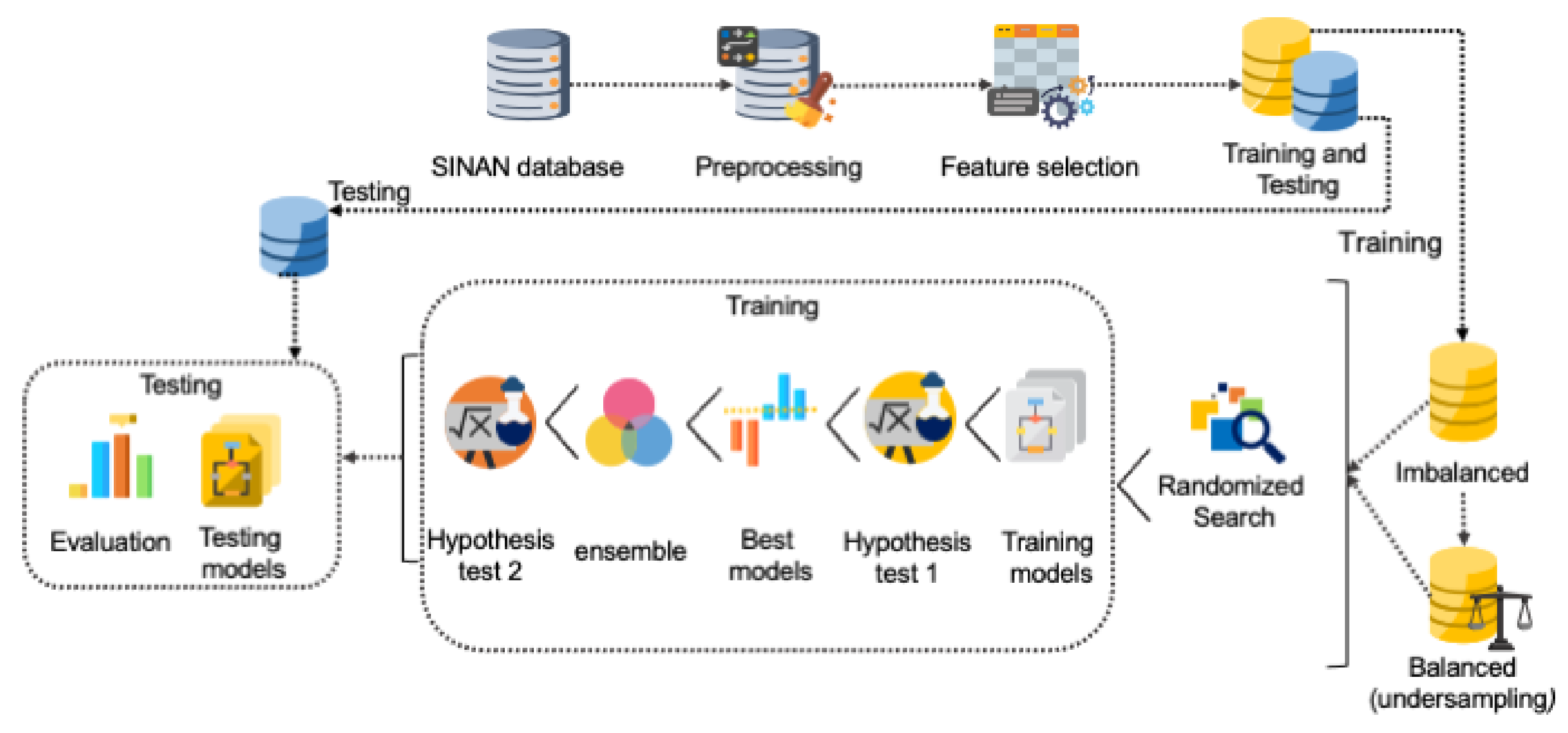
4. Materials and Methods

To benchmark the machine learning models, we followed the methodology presented in Figure 1. The goal was to select the best model to aide TB prognosis. The methodology adopted for this work included preprocessing the data set; applying the feature selection algorithm to reduce the dimensionality of the data set; training the models using an imbalanced data set and a balanced data set; applying randomized search technique to find the best hyperparameters for the models; usage of statistical techniques to determine whether models have similar distributions; finding the best models and generating an ensemble model; usage of statistical techniques to compare the best models; and finally, evaluation of the models through tests.
The SINAN database contained records of patients with diseases listed on the Brazilian National Compulsory Notification List. For the purposes of this work, we used records related to the State of Amazonas from 2007 to 2018 of patients who were diagnosed and treated for TB, the SINAN-TB. In total, the original data set comprised 36,228 records and 130 fields, having 35,007 records of patients cured of TB and 1221 records of TB-related deaths. The description of all fields can be consulted in the SINAN data dictionaries [70].
To clean the data, preprocessing was performed. After the preprocessing, the revised data set included 24,015 records with 38 fields; 22,876 records of patients cured of TB and 1139 records of TB-related deaths.
We compared the performance of four feature selection techniques (SFS, SFFS, SBS and SBFS as per Section 3.1) to select the most representative fields in the original data set. We then reduced the dimensionality of the data to be handled by the models. 17 fields were selected for each of the nine machine learning models. This is consistent with [44] where the same SINAN-TB data set was used and features selected by a specialist. We used the entire data set and applied k-fold cross validation, with k = 10 as per [71,72,73,74].
As per the original data set, the preprocessed data set was imbalanced (22,876 cured patients and 1139 TB mortalities). As such, two scenarios were designed for experiments and evaluations: (1) using the revised imbalanced data set, and (2) using a balanced-version of the revised data set as per [75]. To create the balanced data set, the random under-sampling technique was applied and a balanced data set was generated comprising 1139 records of patients cured of TB and 1139 mortalities. The data set was then split between training and validation (70%) and testing (30%).
For both scenarios, the randomized search hyperparameter optimizer was applied using the parameters and configurations available in the sci-kit learn library for Python (https://scikit-learn.org/stable/supervised_learning.html#supervised-learning (accessed on 14 April 2021)). The randomized search technique set up a grid of hyperparameter values and selected random combinations to train a given model [76]. Randomized search can outperform a grid search [76], especially if only a small number of hyperparameters is used to compare the performance of the machine learning model. Having selected the hyperparameter configuration of each model, the models were trained as explained previously and the average of the F1-macro metric was calculated.
The Wilcoxon hypothesis test was performed to eliminate models with similar distributions and compose the ensemble model. The Wilcoxon test is a non-parametric test used to test the hypothesis that the probability distribution of the first sample is equal to the probability distribution of the second sample [77]. We assumed an F1-macro greater than or equal to 80% as the criterion to decide which model should be eliminated to compose the ensemble model. By eliminating models with similar distributions or with a performance below 80%, the overall performance of the ensemble model would improve. Consequently, an ensemble model was built with the best models using a stacking classifier. The stacking classifier stacked the outputs of the selected models and used an LR classifier to calculate the final prediction, similar to [78]. Finally, given the best models, the test was performed 10 times and the accuracy, precision, sensitivity, specificity, F1-score, AUC ROC and F1-macro average are calculated for evaluation.

5. Results

All the computation processing (database preprocessing, feature selection, grid search, and training and test of the models) was done using an AWS instance, i3en.6xlarge. The configuration included 24 3.1 GHz vCPUs, core turbo Intel Xeon Scalable processors, and 192 GB of memory.

5.1. Preprocessing and Feature Selection

As described in Section 4, after applying the data preprocessing steps, the revised data set comprised 38 fields. As discussed earlier, Rocha et al. [44] used the same SINAN-TB data set with 17 fields selected by a specialist to predict TB. In our work, for the application of the feature selection techniques, the same number of fields was defined. We executed the four feature selection techniques, SFS, SBS, SFFS and SBFS, under k-fold cross-validation (with k = 10 ), using the nine machine learning models.
Table 1 presents the average of the F1-score of each feature selection technique. DT presented the best F1-score (96.00%) when using the SFS technique; LDA presented the best F1-score (95.31%) when using the SBS technique; KNN, NB, SVM and RF presented the best F1-score, 95.40%, 94.39%, 95.23% and 94.84%, respectively, when using the SFFS technique; and LR, GB and MLP presented the best F1-score, 95.31%, 96.30% and 95.72%, respectively, when using the SBFS technique. It is worth noting that SFFS achieved the best result for four of the nine models, followed by SBFS.
While the SFFS and SBFS techniques presented the best results for most of the machine learning models, these techniques are computationally more costly. While SFS took 8.69 h to run all the experiments, SFFS took 26.15 h. Similarly, while SBS took 20.09 h, SBFS took 30.97 h.
For each machine learning model, we selected the feature selection technique that produced the best F1-score. These are presented with respective fields in Table 2. The field “DIAS” (days of hospitalization for which the patient was treated ) was selected by all models. “BACILOSC_6” (result of sputum smear microscopy for bacillus alcohol resistance) and “IDADE” (patient age) were the fields selected by eight and seven of the machine learning models, respectively. On the other hand, the fields “BACILOS_E2” (results of sputum smear microscopy for acid-resistant bacillus performed on a sample for diagnosis) and “ESTREPTOMI” (Etionamide drugs) were selected by only one model.

5.2. Results of the Randomized Search Technique

Table 3 presents the best configuration for each model achieved by the randomized search technique for both scenarios (imbalanced and balanced data sets) assuming the F1-macro as evaluation metric. These configurations were used to execute the training and testing of the models.
Selected hyperparameters may change when using imbalanced and balanced data sets. SVM, GB, RF and MLP models kept the same hyperparameter configuration in both cases. For more details about the parameters and configurations, please refer to the scikit-learn library.

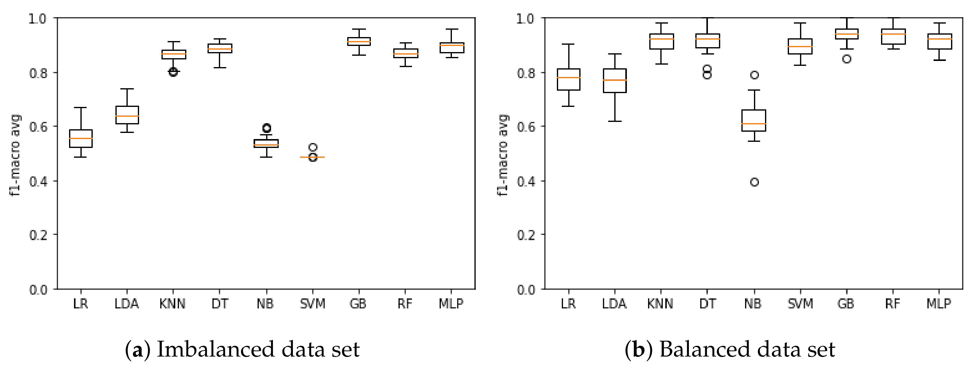
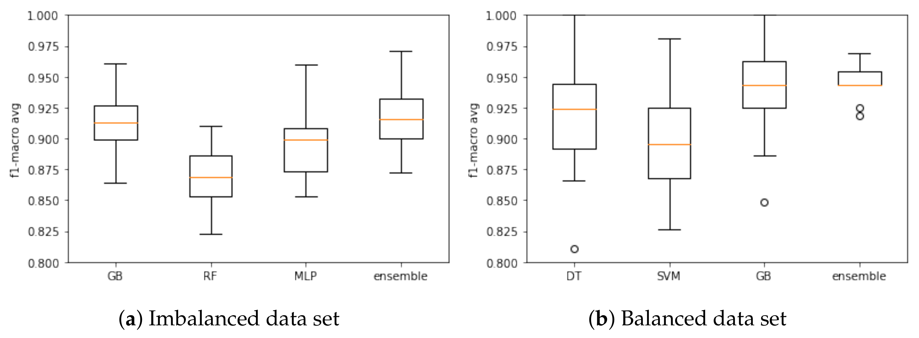
5.3. Model Training and Validation

Figure 2a presents the results of the model training based on the F1-macro metric when using the imbalanced data set. The model that obtained the best mean F1-macro was GB with 91.14%, and the poorest performing was SVM with 48.88%. Figure 2b presents the results of the model training based on the F1-macro metric when using the balanced data set. The model that obtained the best mean F1-macro was GB with 94.52%, and the poorest performing was NB with 62.39%.
Based on the F1-macro results, the Wilcoxon test was applied to identify the models with similar distributions and discard the models with the lowest results. When using the imbalanced data set, KNN, DT and RF models presented similar distributions, and then KNN and DT were discarded. LR, LDA, NB and SVM models were discarded as they had the lowest results. Therefore, RF, GB and MLP models were selected to compose the ensemble model based on the imbalanced database. Figure 3a presents the results of these models based on the F1-macro and the imbalanced data set.
With respect to the balanced data set, the following models presented similar distribution: LR and LDA; KNN, DT and MLP; GB and RF. In this case, LR, KNN, MLP and RF models were discarded. The LDA and NB models were discarded due low F1-macro results. Three models were selected to compose the ensemble model in this case: DT, SVM and GB. Figure 3b presents the results when using the balanced data set.
Again, the Wilcoxon hypothesis test was executed. For the imbalanced data set, no model had a similar distribution, so all models remained for the testing step. The ensemble was the best model (F1-macro mean of 91.69%). For the balanced data set, no model had a similar distribution, so DT, SVM and GB remained for the testing step. The ensemble was the best model (F1-macro mean of 94.52%). Results are summarized in Table 4.

5.4. Testing the Models

Using the models that presented the best performance during the training step, we test them using the 30% of the data set not used during model training. Table 5 and Table 6 present the test results of each model for imbalanced and balanced data sets, respectively.
For the imbalanced data set, the RF and ensemble model presented the best mean for three metrics. RF performed better in precision (99.58%), sensitivity (91.50%) and AUC ROC (94.41%), while the ensemble model performed better in accuracy (98.57%), F1-score (99.25%) and F1-macro (91.46%). The best specificity was obtained by the GB, and the MLP performed worst across all metrics tested.
When using the balanced data set, the GB model performed best of those tested. Notwithstanding this, it is worth noting that the DT, SVM and ensemble models presented very similar results to the GB. The ensemble model performance can be explained by its composition based on the DT, SVM and GB models.

5.5. Discussion

The impact of imbalanced and balanced data sets on model performance during the training phase can be easily observed (Figure 2a). In general, models trained with the balanced data set achieved superior results (Figure 2b). When the models were tested (Table 5), the GB and ensemble models (composed of the RF, GB and MLP models) presented the best performance in relation to the F1-macro metric using the imbalanced data set, and the GB model presented the best sensitivity when using the balanced data set.
For discussion purposes, we selected a confusion matrix for each model as an example. Table 7 presents the confusion matrices of the best performing models when using the imbalanced data set i.e., GB, RF, MLP and ensemble. The ensemble model classified 6700 cases correctly as cured TB patients and 302 as TB deaths; 29 cases were incorrectly classified as cured TB patients and 174 cases incorrectly classified as mortalities. The RF model presented the worst FP results, predicting 178 TB mortalities as cured TB patients. GB was the model with the worst FN results, predicting 71 TB-related mortalities as cured TB patients.
Table 8 presents the confusion matrices of the models that presented the best performance when using the balanced data set. As the GB model presented the best results (see Table 6), this is reflected in its confusion matrix. In this example, the GB model classified 6596 cases correctly as cured TB patients and 322 cases as TB mortalities; 278 cases were incorrectly classified as mortalities and only nine incorrectly classified as cured TB patients. The model with the best FP results was the DT with 617 cases predicted as TB-related mortalities. The model with the best FN results was the SVM with 55 deaths predicted as cured TB patients.
These confusion matrices can help explain the earlier discussion regarding the performance metrics. In the imbalanced data set, the RF and ensemble models achieved relatively strong results. For the balanced data set, the GB model outperformed all the other models. When comparing the results of the balanced and imbalanced data sets, we found the ensemble model presented the best F1-macro score. However, in the context of TB prognosis, this involves the possibility of patient TB-mortality if untreated, an unacceptable outcome. The performance of the GB model when using the balanced database is noteworthy-it achieved 97.50% in sensitivity on average, or as seen in Table 8, it classified only nine deaths erroneously as a TB patient. In a TB prognosis, treating a patient who subsequently dies from TB is more acceptable than not treating a TB patient who may recover. As such, in our opinion, the GB presents the best performance for the TB-mortality prognosis use case in balanced data set, and the ensemble model presents the best performance for the TB cured prognosis in the imbalanced data set.
As discussed, comparisons with previous studies are difficult due to the difference and availability of reference data sets. For example, Kalhori et al. [42] used a data set with 6450 cases of TB from Iran to classify the outcome of a course of TB treatment. Their results suggested their DT model presented the best performance with 74.21% accuracy, 74.20% sensitivity, 75.30% precision, 74.60% F1-score, and 97.00% of AUC ROC. Our DT model outperformed their DT model in all these metrics and in both data set scenarios (imbalanced and balanced), with exception of the AUC ROC where our result was lower at 92.90%. Regarding the other models, our SVM and MLP also presented better performance than the respective models evaluated by Kalhori et al. [42].

6. Conclusions

There is an established literature based on the use of machine learning for the detection of TB diagnosis. In contrast, there is a dearth of research on the use of machine learning for the prognosis of TB, a critical factor in effective TB treatment. In this paper, we addressed an important gap in the literature by benchmarking several machine learning models to aide TB prognosis and associated decision making. An ensemble model was also proposed considering heterogeneous classifiers; it presented the best performance.
We evaluated two data set scenarios—an imbalanced data set and a balanced data set. For the former, the GB model achieved the best mean specificity at 99.50%. The RF model achieved the best precision mean at 99.58%, sensitivity at 91.50%, and AUC ROC at 94.41%. An ensemble model composed of RF, GB and MLP models achieved the best mean accuracy at 98.57%, F1-score at 99.25%, and F1-macro at 91.45%. When using the balanced data set, the GB model achieved the best mean in all metrics: 95.97% accuracy, 99.86% precision, 95.91% specificity, 97.22% sensitivity, 97.84% F1-score, 96.56% AUC ROC, and 84.40% F1-macro. Based on these results, data set preprocessing impacted directly on the performance of the models.
For future research, we plan to study one-class classification methods and analyze the usage of other algorithms, including deep learning and deep learning ensembles, to improve the hyperparameter tuning for models and the selection of the best fields to be used as the input for the models. Hemingway et al. [10] raises significant issues on the quality of prognosis research and underlying biases. Machine learning can be used to augment human decision making. As such, we also plan to develop a framework composed of the best models to assist health professionals in the treatment of TB. This framework will inform decision support system in the form of a mobile application so that physicians, particularly those working remotely in the field, can use our models to support their decisions regarding post-diagnosis treatment.

Author Contributions

Conceptualization, M.H.L.F.d.S.B., V.S. and P.T.E.; methodology, M.H.L.F.d.S.B. and P.T.E.; software, M.H.L.F.d.S.B., L.M.F.S., E.d.S.R. and G.O.A.; validation, J.F.L.d.O., T.L. and P.T.E.; formal analysis, M.H.L.F.d.S.B., E.d.S.R., V.S. and P.T.E.; investigation, M.H.L.F.d.S.B., J.F.L.d.O., V.S. and P.T.E.; resources, M.H.L.F.d.S.B.; data curation, M.H.L.F.d.S.B.; writing—original draft preparation, M.H.L.F.d.S.B., L.M.F.S., and G.O.A.; writing—review and editing, M.H.L.F.d.S.B., E.d.S.R., J.F.L.d.O., T.L., V.S. and P.T.E.; supervision, J.F.L.d.O., T.L., V.S. and P.T.E.; project administration, P.T.E. and V.S.. All authors have read and agreed to the published version of the manuscript.

Funding

This research received no external funding.

Institutional Review Board Statement

Not applicable.

Informed Consent Statement

Not applicable.

Data Availability Statement

The data used in this work were extracted from SINAN-TB, and are only available under formal consultation and authorization from the Brazilian ethics committee.

Acknowledgments

We thank the Coordenação de Aperfeiçoamento de Pessoal de Nível Superior—Brasil (CAPES), the National Council for Scientific, Technological Development (CNPq) and the Fundação de Amparo à Pesquisa do Estado do Amazonas (PAPAC 005/2019, PRÓ-ESTADO, and Posgrad calls) and the Irish Institute of Digital Business (IIDB) at DCU.

Conflicts of Interest

The authors declare no conflict of interest.

References

  1. Pai, M.; Behr, M.; Dowdy, D.; Dheda, K.; Divangahi, M.; Boehme, C.; Raviglione, M. Tuberculosis. Nat. Rev. Dis. Prim. 2016, 2, 16076. [Google Scholar] [CrossRef]
  2. WHO. Global Tuberculosis Report 2020. Available online: https://apps.who.int/iris/bitstream/handle/10665/336069/9789240013131-eng.pdf (accessed on 25 January 2021).
  3. Tuberculosis Profile: Brazil. Available online: https://worldhealthorg.shinyapps.io/tb_profiles?_inputs_&lan=%22EN%22&iso2=%22BR%22 (accessed on 25 September 2020).
  4. WHO. Country Profiles for 30 High TB Burden Countries. Available online: https://www.who.int/tb/publications/global_report/tb19_Report_country_profiles_15October2019.pdf?ua=1 (accessed on 29 September 2020).
  5. Ranzani, O.T.; Pescarini, J.M.; Martinez, L.; Garcia-Basteiro, A.L. Increasing tuberculosis burden in Latin America: An alarming trend for global control efforts. BMJ 2021. [Google Scholar] [CrossRef]
  6. Sistema Único de Saúde (SUS): Estrutura, Princípios e Como Funciona. Available online: https://antigo.saude.gov.br/sistema-unico-de-saude (accessed on 25 January 2021).
  7. Brasil é único com ‘SUS’ Entre Países Com Mais de 200 Milhões de Habitantes. Available online: https://www1.folha.uol.com.br/cotidiano/2019/10/brasil-e-unico-com-sus-entre-paises-com-mais-de-200-milhoes-de-habitantes.shtml (accessed on 28 January 2021).
  8. Brazil’s Sistema Único da Saúde (SUS): Caught in the Cross Fire. Available online: https://www.csis.org/blogs/smart-global-health/brazils-sistema-unico-da-saude-sus-caught-cross-fire (accessed on 25 January 2021).
  9. Hemingway, H. Prognosis research: Why is Dr. Lydgate still waiting? J. Clin. Epidemiol. 2006, 59, 1229–1238. [Google Scholar] [CrossRef]
  10. Hemingway, H.; Riley, R.D.; Altman, D.G. Ten steps towards improving prognosis research. BMJ 2009, 339, b4184. [Google Scholar] [CrossRef] [PubMed]
  11. Bora, R.M.; Chaudhari, S.N.; Mene, S.P. A Review of Ensemble Based Classification and Clustering in Machine Learning. Int. J. New Innov. Eng. Technol. 2019, 12, 2319–6319. [Google Scholar]
  12. García-Gil, D.; Holmberg, J.; García, S.; Xiong, N.; Herrera, F. Smart Data based Ensemble for Imbalanced Big Data Classification. arXiv 2020, arXiv:2001.05759. [Google Scholar]
  13. Yang, K.; Yu, Z.; Wen, X.; Cao, W.; Chen, C.P.; Wong, H.S.; You, J. Hybrid Classifier Ensemble for Imbalanced Data. IEEE Trans. Neural Netw. Learn. Syst. 2019, 31, 1387–1400. [Google Scholar] [CrossRef] [PubMed]
  14. Martins, V.d.O.; de Miranda, C.V. Diagnóstico e Tratamento Medicamentoso Em Casos de Tuberculose Pulmonar: Revisão de Literatura. Rev. Saúde Multidiscip. 2020, 7, 1. [Google Scholar]
  15. Lakhani, P.; Sundaram, B. Deep learning at chest radiography: Automated classification of pulmonary tuberculosis by using convolutional neural networks. Radiology 2017, 284, 574–582. [Google Scholar] [CrossRef] [PubMed]
  16. Rajaraman, S.; Candemir, S.; Xue, Z.; Alderson, P.O.; Kohli, M.; Abuya, J.; Thoma, G.R.; Antani, S. A novel stacked generalization of models for improved TB detection in chest radiographs. In Proceedings of the 2018 40th Annual International Conference of the IEEE Engineering in Medicine and Biology Society (EMBC), Honolulu, HI, USA, 18–21 July 2018; pp. 718–721. [Google Scholar]
  17. Hooda, R.; Sofat, S.; Kaur, S.; Mittal, A.; Meriaudeau, F. Deep-learning: A potential method for tuberculosis detection using chest radiography. In Proceedings of the 2017 IEEE International Conference on Signal and Image Processing Applications (ICSIPA), Kuching, Malaysia, 12–14 September 2017; pp. 497–502. [Google Scholar]
  18. Sethi, K.; Parmar, V.; Suri, M. Low-Power Hardware-Based Deep-Learning Diagnostics Support Case Study. In Proceedings of the 2018 IEEE Biomedical Circuits and Systems Conference (BioCAS), Cleveland, OH, USA, 17–19 October 2018; pp. 1–4. [Google Scholar]
  19. Kant, S.; Srivastava, M.M. Towards automated tuberculosis detection using deep learning. In Proceedings of the 2018 IEEE Symposium Series on Computational Intelligence (SSCI), Bangalore, India, 18–21 November 2018; pp. 1250–1253. [Google Scholar]
  20. Carneiro, G.; Oakden-Rayner, L.; Bradley, A.P.; Nascimento, J.; Palmer, L. Automated 5-year mortality prediction using deep learning and radiomics features from chest computed tomography. In Proceedings of the 2017 IEEE 14th International Symposium on Biomedical Imaging (ISBI 2017), Melbourne, VIC, Australia, 18–21 April 2017; pp. 130–134. [Google Scholar]
  21. Song, Q.; Zheng, Y.J.; Xue, Y.; Sheng, W.G.; Zhao, M.R. An evolutionary deep neural network for predicting morbidity of gastrointestinal infections by food contamination. Neurocomputing 2017, 226, 16–22. [Google Scholar] [CrossRef]
  22. Lee, C.K.; Hofer, I.; Gabel, E.; Baldi, P.; Cannesson, M. Development and validation of a deep neural network model for prediction of postoperative in-hospital mortality. Anesthesiol. J. Am. Soc. Anesthesiol. 2018, 129, 649–662. [Google Scholar] [CrossRef] [PubMed]
  23. Peetluk, L.S.; Ridolfi, F.M.; Rebeiro, P.F.; Liu, D.; Rolla, V.C.; Sterling, T.R. Systematic review of prediction models for pulmonary tuberculosis treatment outcomes in adults. BMJ Open 2021, 11, e044687. [Google Scholar] [CrossRef] [PubMed]
  24. Abdelbary, B.; Garcia-Viveros, M.; Ramirez-Oropesa, H.; Rahbar, M.; Restrepo, B. Predicting treatment failure, death and drug resistance using a computed risk score among newly diagnosed TB patients in Tamaulipas, Mexico. Epidemiol. Infect. 2017, 145, 3020–3034. [Google Scholar] [CrossRef] [Green Version]
  25. Aljohaney, A.A. Mortality of patients hospitalized for active tuberculosis in King Abdulaziz University Hospital, Jeddah, Saudi Arabia. Saudi Med. J. 2018, 39, 267. [Google Scholar] [CrossRef] [PubMed]
  26. Bastos, H.N.; Osório, N.S.; Castro, A.G.; Ramos, A.; Carvalho, T.; Meira, L.; Araújo, D.; Almeida, L.; Boaventura, R.; Fragata, P.; et al. A prediction rule to stratify mortality risk of patients with pulmonary tuberculosis. PLoS ONE 2016, 11, e0162797. [Google Scholar] [CrossRef] [Green Version]
  27. Gupta-Wright, A.; Corbett, E.L.; Wilson, D.; van Oosterhout, J.J.; Dheda, K.; Huerga, H.; Peter, J.; Bonnet, M.; Alufandika-Moyo, M.; Grint, D.; et al. Risk score for predicting mortality including urine lipoarabinomannan detection in hospital inpatients with HIV-associated tuberculosis in sub-Saharan Africa: Derivation and external validation cohort study. PLoS Med. 2019, 16, e1002776. [Google Scholar] [CrossRef]
  28. Horita, N.; Miyazawa, N.; Yoshiyama, T.; Sato, T.; Yamamoto, M.; Tomaru, K.; Masuda, M.; Tashiro, K.; Sasaki, M.; Morita, S.; et al. Development and validation of a tuberculosis prognostic score for smear-positive in-patients in Japan. Int. J. Tuberc. Lung Dis. 2013, 17, 54–60. [Google Scholar] [CrossRef]
  29. Koegelenberg, C.F.N.; Balkema, C.A.; Jooste, Y.; Taljaard, J.J.; Irusen, E.M. Validation of a severity-of-illness score in patients with tuberculosis requiring intensive care unit admission. S. Afr. Med. J. 2015, 105, 389–392. [Google Scholar] [CrossRef] [Green Version]
  30. Nguyen, D.T.; Graviss, E.A. Development and validation of a prognostic score to predict tuberculosis mortality. J. Infect. 2018, 77, 283–290. [Google Scholar] [CrossRef] [Green Version]
  31. Nguyen, D.T.; Graviss, E.A. Development and validation of a risk score to predict mortality during TB treatment in patients with TB-diabetes comorbidity. BMC Infect. Dis. 2019, 19, 1–8. [Google Scholar] [CrossRef]
  32. Nguyen, D.T.; Jenkins, H.E.; Graviss, E.A. Prognostic score to predict mortality during TB treatment in TB/HIV co-infected patients. PLoS ONE 2018, 13, e0196022. [Google Scholar] [CrossRef] [PubMed] [Green Version]
  33. Pefura-Yone, E.W.; Balkissou, A.D.; Poka-Mayap, V.; Fatime-Abaicho, H.K.; Enono-Edende, P.T.; Kengne, A.P. Development and validation of a prognostic score during tuberculosis treatment. BMC Infect. Dis. 2017, 17, 251. [Google Scholar] [CrossRef] [PubMed] [Green Version]
  34. Podlekareva, D.N.; Grint, D.; Post, F.A.; Mocroft, A.; Panteleev, A.M.; Miller, R.; Miro, J.; Bruyand, M.; Furrer, H.; Riekstina, V.; et al. Health care index score and risk of death following tuberculosis diagnosis in HIV-positive patients. Int. J. Tuberc. Lung Dis. 2013, 17, 198–206. [Google Scholar] [CrossRef] [Green Version]
  35. Valade, S.; Raskine, L.; Aout, M.; Malissin, I.; Brun, P.; Deye, N.; Baud, F.J.; Megarbane, B. Tuberculosis in the intensive care unit: A retrospective descriptive cohort study with determination of a predictive fatality score. Can. J. Infect. Dis. Med. Microbiol. 2012, 23, 173–178. [Google Scholar] [CrossRef] [PubMed] [Green Version]
  36. Wang, Q.; Han, W.; Niu, J.; Sun, B.; Dong, W.; Li, G. Prognostic value of serum macrophage migration inhibitory factor levels in pulmonary tuberculosis. Respir. Res. 2019, 20, 1–10. [Google Scholar] [CrossRef] [PubMed] [Green Version]
  37. Wejse, C.; Gustafson, P.; Nielsen, J.; Gomes, V.F.; Aaby, P.; Andersen, P.L.; Sodemann, M. TBscore: Signs and symptoms from tuberculosis patients in a low-resource setting have predictive value and may be used to assess clinical course. Scand. J. Infect. Dis. 2008, 40, 111–120. [Google Scholar] [CrossRef]
  38. Zhang, Z.; Xu, L.; Pang, X.; Zeng, Y.; Hao, Y.; Wang, Y.; Wu, L.; Gao, G.; Yang, D.; Zhao, H.; et al. A Clinical scoring model to predict mortality in HIV/TB co-infected patients at end stage of AIDS in China: An observational cohort study. Biosci. Trends 2019, 13, 136–144. [Google Scholar] [CrossRef] [PubMed]
  39. Hussain, O.A.; Junejo, K.N. Predicting treatment outcome of drug-susceptible tuberculosis patients using machine-learning models. Inform. Health Soc. Care 2019, 44, 135–151. [Google Scholar] [CrossRef]
  40. Killian, J.A.; Wilder, B.; Sharma, A.; Choudhary, V.; Dilkina, B.; Tambe, M. Learning to prescribe interventions for tuberculosis patients using digital adherence data. In Proceedings of the 25th ACM SIGKDD International Conference on Knowledge Discovery & Data Mining, Anchorage, AK, USA, 4–8 August 2019; pp. 2430–2438. [Google Scholar]
  41. Sauer, C.M.; Sasson, D.; Paik, K.E.; McCague, N.; Celi, L.A.; Sanchez Fernandez, I.; Illigens, B.M. Feature selection and prediction of treatment failure in tuberculosis. PLoS ONE 2018, 13, e0207491. [Google Scholar] [CrossRef]
  42. Kalhori, S.R.N.; Zeng, X.J. Evaluation and comparison of different machine learning methods to predict outcome of tuberculosis treatment course. J. Intell. Learn. Syst. Appl. 2013, 5, 10. [Google Scholar] [CrossRef] [Green Version]
  43. Kira, K.; Rendell, L.A. A practical approach to feature selection. In Machine Learning Proceedings 1992; Elsevier: Amsterdam, The Netherlands, 1992; pp. 249–256. [Google Scholar]
  44. Rocha, E.D.S. DEEPTUB: Plataforma Para PrediçãO De Morte Por Tuberculose Baseado Em Modelos De Deep Learning Utilizando Dados DemográFicos, ClíNicos E Laboratoriais. Dissertação de Mestrado, Universidade de Pernambuco, Recife, PE, Brazil, 2020. [Google Scholar]
  45. Marcano-Cedeno, A.; Quintanilla-Domínguez, J.; Cortina-Januchs, M.; Andina, D. Feature selection using sequential forward selection and classification applying artificial metaplasticity neural network. In Proceedings of the IECON 2010—36th Annual Conference on IEEE Industrial Electronics Society, Glendale, AZ, USA, 7–10 November 2010; pp. 2845–2850. [Google Scholar]
  46. Alakuş, T.B.; Türkoğlu, İ. Feature selection with sequential forward selection algorithm from emotion estimation based on EEG signals. Sak. Üniversitesi Fen Bilim. Enstitüsü derg. 2019, 23, 1096–1105. [Google Scholar] [CrossRef]
  47. Kuchibhotla, S.; Vankayalapati, H.D.; Anne, K.R. An optimal two stage feature selection for speech emotion recognition using acoustic features. Int. J. Speech Technol. 2016, 19, 657–667. [Google Scholar] [CrossRef]
  48. Varma, M.; Jereesh, A. Identifying predominant clinical and genomic features for glioblastoma multiforme using sequential backward selection. In Proceedings of the 2017 International Conference on Circuit, Power and Computing Technologies (ICCPCT), Kollam, India, 20–21 April 2017; pp. 1–4. [Google Scholar]
  49. Lingampeta, D.; Yalamanchili, B. Human Emotion Recognition using Acoustic Features with Optimized Feature Selection and Fusion Techniques. In Proceedings of the 2020 International Conference on Inventive Computation Technologies (ICICT), Coimbatore, India, 26–28 February 2020; pp. 221–225. [Google Scholar]
  50. Das, K.; Behera, R.N. A survey on machine learning: Concept, algorithms and applications. Int. J. Innov. Res. Comput. Commun. Eng. 2017, 5, 1301–1309. [Google Scholar]
  51. Callahan, A.; Shah, N.H. Machine learning in healthcare. In Key Advances in Clinical Informatics; Elsevier: Amsterdam, The Netherlands, 2017; pp. 279–291. [Google Scholar]
  52. Bonte, C.; Vercauteren, F. Privacy-preserving logistic regression training. BMC Med. Genom. 2018, 11, 86. [Google Scholar] [CrossRef] [PubMed]
  53. Menard, S. Applied Logistic Regression Analysis; SAGE: Thousand Oaks, CA, USA, 2002; Volume 106. [Google Scholar]
  54. Fisher, R.A. The use of multiple measurements in taxonomic problems. Ann. Eugen. 1936, 7, 179–188. [Google Scholar] [CrossRef]
  55. Xanthopoulos, P.; Pardalos, P.M.; Trafalis, T.B. Linear discriminant analysis. In Robust Data Mining; Springer: Berlin/Heidelberg, Germany, 2013; pp. 27–33. [Google Scholar]
  56. Balakrishnama, S.; Ganapathiraju, A. Linear discriminant analysis-a brief tutorial. Inst. Signal Inf. Process. 1998, 18, 1–8. [Google Scholar]
  57. Basha, S.M.; Rajput, D.S. Survey on Evaluating the Performance of Machine Learning Algorithms: Past Contributions and Future Roadmap. In Deep Learning and Parallel Computing Environment for Bioengineering Systems; Elsevier: Amsterdam, The Netherlands, 2019; pp. 153–164. [Google Scholar]
  58. Guo, G.; Wang, H.; Bell, D.; Bi, Y.; Greer, K. KNN model-based approach in classification. In OTM Confederated International Conferences “On the Move to Meaningful Internet Systems”; Springer: Berlin/Heidelberg, Germany, 2003; pp. 986–996. [Google Scholar]
  59. Talita, A.; Nataza, O.; Rustam, Z. Naïve Bayes Classifier and Particle Swarm Optimization Feature Selection Method for Classifying Intrusion Detection System Dataset. J. Phys. Conf. Ser. IOP Publ. 2021, 1752, 012021. [Google Scholar] [CrossRef]
  60. Rukmawan, S.; Aszhari, F.; Rustam, Z.; Pandelaki, J. Cerebral Infarction Classification Using the K-Nearest Neighbor and Naive Bayes Classifier. J. Phys. Conf. Ser. 2021, 1752, 012045. [Google Scholar] [CrossRef]
  61. Rish, I. An empirical study of the naive Bayes classifier. In Proceedings of the IJCAI 2001 Workshop On Empirical Methods in Artificial Intelligence, Seattle, WA, USA, 4–6 August 2001; Volume 3, pp. 41–46. [Google Scholar]
  62. da Silva, L.A.; Peres, S.M.; Boscarioli, C. Introdução à Mineração de Dados: Com Aplicações em R; Elsevier: Brasil, Brazil, 2017. [Google Scholar]
  63. Bordoloi, D.J.; Tiwari, R. Optimum multi-fault classification of gears with integration of evolutionary and SVM algorithms. Mech. Mach. Theory 2014, 73, 49–60. [Google Scholar] [CrossRef]
  64. Yao, Y.; Liu, Y.; Yu, Y.; Xu, H.; Lv, W.; Li, Z.; Chen, X. K-SVM: An Effective SVM Algorithm Based on K-means Clustering. JCP 2013, 8, 2632–2639. [Google Scholar] [CrossRef]
  65. Lu, H.; Karimireddy, S.P.; Ponomareva, N.; Mirrokni, V. Accelerating Gradient Boosting Machines. In Proceedings of the International Conference on Artificial Intelligence and Statistics, PMLR, Palermo, Italy, 3–5 June 2020; pp. 516–526. [Google Scholar]
  66. Natekin, A.; Knoll, A. Gradient boosting machines, a tutorial. Front. Neurorobot. 2013, 7, 21. [Google Scholar] [CrossRef] [PubMed] [Green Version]
  67. Gomes, H.M.; Bifet, A.; Read, J.; Barddal, J.P.; Enembreck, F.; Pfharinger, B.; Holmes, G.; Abdessalem, T. Adaptive random forests for evolving data stream classification. Mach. Learn. 2017, 106, 1469–1495. [Google Scholar] [CrossRef]
  68. Zanaty, E. Support vector machines (SVMs) versus multilayer perception (MLP) in data classification. Egypt. Inform. J. 2012, 13, 177–183. [Google Scholar] [CrossRef]
  69. Zhou, Z.H. Ensemble Methods: Foundations and Algorithms; CRC Press: Boca Raton, FL, USA, 2012. [Google Scholar]
  70. Dicionário de Dados-SINAN NET-Versão 5.0. Available online: http://portalsinan.saude.gov.br/images/documentos/Agravos/Tuberculose/DICI_DADOS_NET_Tuberculose_23_07_2020.pdf (accessed on 25 January 2021).
  71. Badža, M.M.; Barjaktarović, M.Č. Classification of brain tumors from MRI images using a convolutional neural network. Appl. Sci. 2020, 10, 1999. [Google Scholar] [CrossRef] [Green Version]
  72. Cherifa, M.; Blet, A.; Chambaz, A.; Gayat, E.; Resche-Rigon, M.; Pirracchio, R. Prediction of an acute hypotensive episode during an ICU hospitalization with a super learner machine-learning algorithm. Anesth. Analg. 2020, 130, 1157–1166. [Google Scholar] [CrossRef] [PubMed]
  73. Song, W.; Jung, S.Y.; Baek, H.; Choi, C.W.; Jung, Y.H.; Yoo, S. A Predictive Model Based on Machine Learning for the Early Detection of Late-Onset Neonatal Sepsis: Development and Observational Study. JMIR Med. Inform. 2020, 8, e15965. [Google Scholar] [CrossRef] [PubMed]
  74. Eickelberg, G.; Sanchez-Pinto, L.N.; Luo, Y. Predictive modeling of bacterial infections and antibiotic therapy needs in critically ill adults. J. Biomed. Inform. 2020, 109, 103540. [Google Scholar] [CrossRef]
  75. Ho Thanh Lam, L.; Le, N.H.; Van Tuan, L.; Tran Ban, H.; Nguyen Khanh Hung, T.; Nguyen, N.T.K.; Huu Dang, L.; Le, N.Q.K. Machine learning model for identifying antioxidant proteins using features calculated from primary sequences. Biology 2020, 9, 325. [Google Scholar] [CrossRef]
  76. Liashchynskyi, P.; Liashchynskyi, P. Grid Search, Random Search, Genetic Algorithm: A Big Comparison for NAS. arXiv 2019, arXiv:1912.06059. [Google Scholar]
  77. Woolson, R. Wilcoxon signed-rank test. In Wiley Encyclopedia of Clinical Trials; John Wiley & Sons, Inc.: Hoboken, NJ, USA, 2007; pp. 1–3. [Google Scholar]
  78. Le, N.Q.K.; Do, D.T.; Hung, T.N.K.; Lam, L.H.T.; Huynh, T.T.; Nguyen, N.T.K. A computational framework based on ensemble deep neural networks for essential genes identification. Int. J. Mol. Sci. 2020, 21, 9070. [Google Scholar] [CrossRef]
Figure 1. Methodology used to benchmark machine learning models.
Informatics 08 00027 g001
Figure 2. F1-macro results for the machine learning model training when using the (a) imbalanced and (b) balanced data set.
Informatics 08 00027 g002
Figure 3. Ensemble model training and associated models based on the (a) imbalanced and (b) balanced data. sets.
Informatics 08 00027 g003
Table 1. Results of F1-score (in %) and the respective standard deviation related to the feature selection techniques for each machine learning model.
Feature Selection Techniques
ModelSFSSFFSSBSSBFS
LR 94.71 (±0.007)94.88 (±0.007)95.30 (±0.000)95.31 (±0.000)
LDA 94.94 (±0.007)95.13 (±0.006)95.31 (±0.001)95.30 (±0.001)
KNN 95.17 (±0.004)95.40 (±0.002)93.79 (±0.004)93.89 (±0.005)
DT 96.00 (±0.002)95.99 (±0.002)95.71 (±0.001)95.70 (±0.001)
NB 94.11 (±0.003)94.39 (±0.001)90.15 (±0.004)90.15 (±0.004)
SVM 95.22 (±0.002)95.23 (±0.002)94.37 (±0.002)94.38 (±0.002)
GB 96.04 (±0.003)96.02 (±0.003)96.29 (±0.000)96.30 (±0.000)
RF 94.63 (±0.006)94.84 (±0.006)92.69 (±0.005)92.74 (±0.005)
MLP 95.51 (±0.004)95.55 (±0.003)95.70 (±0.000)95.72 (±0.000)
Table 2. Features selected through the best F1-score average of feature selection techniques.
SBFSSBSSFFSSFSSFFSSFFSSBFSSFFSSBFS
LR LDA KNN DT NB SVM GB RF MLP 
CS_SEXOCS_SEXOFORMACS_SEXOCS_SEXOCS_SEXOTRATAMENTOCS_SEXORAIOX_TORA
CS_RACATESTE_TUBEAGRAVDIABECS_RACACS_RACACS_RACAAGRAVAIDSCS_RACAAGRAVALCOO
TRATAMENTOFORMAAGRAVDOENCTRATAMENTOTRATAMENTOTRATAMENTOAGRAVALCOOTRATAMENTOBACILOSC_E
RAIOX_TORAAGRAVAIDSBACILOSC_OTESTE_TUBERAIOX_TORAAGRAVAIDSBACILOSC_ORAIOX_TORACULTURA_ES
FORMAAGRAVALCOORIFAMPICINAGRAVDOENCTESTE_TUBEAGRAVALCOOCULTURA_ESFORMAHIV
AGRAVDIABEAGRAVDIABEISONIAZIDARIFAMPICINAGRAVAIDSAGRAVDIABEHIVAGRAVDIABERIFAMPICIN
BACILOSC_EAGRAVOUTRAETAMBUTOLETAMBUTOLAGRAVALCOOAGRAVDOENCETAMBUTOLAGRAVDOENCISONIAZIDA
BACILOSC_OBACILOSC_EESTREPTOMIPIRAZINAMIAGRAVOUTRABACILOSC_EPIRAZINAMIAGRAVOUTRAETAMBUTOL
RIFAMPICINBACILOS_E2PIRAZINAMIOUTRASBACILOSC_EBACILOSC_OETIONAMIDACULTURA_ESTRAT_SUPER
ETAMBUTOLBACILOSC_OETIONAMIDADOENCA_TRACULTURA_ESHIVBACILOSC_1HIVBACILOSC_1
BACILOSC_1CULTURA_ESOUTRASBACILOSC_2HIVBACILOSC_3BACILOSC_2BACILOSC_1BACILOSC_2
BACILOSC_2DOENCA_TRADOENCA_TRABACILOSC_3OUTRASBACILOSC_4BACILOSC_3BACILOSC_2BACILOSC_4
BACILOSC_3BACILOSC_6BACILOSC_4BACILOSC_4DOENCA_TRABACILOSC_5BACILOSC_5BACILOSC_3BACILOSC_6
BACILOSC_4AGRAVDROGABACILOSC_5BACILOSC_5AGRAVDROGABACILOSC_6BACILOSC_6BACILOSC_6TPUNINOT
BACILOSC_6AGRAVTABACBACILOSC_6BACILOSC_6AGRAVTABACTPUNINOTTPUNINOTTPUNINOTAGRAVTABAC
DIASDIASAGRAVDROGAAGRAVTABACDIASDIASDIASDIASDIAS
IDADEIDADEDIASDIASIDADEIDADEIDADEIDADEIDADE
Table 3. Hyperparameter configuration selected by the randomized search technique.
ModelParametersRandomized
Search Using
Imbalanced Data Set
Randomized
Search Using
Balanced Data Set
LRPenaltynonel1
Solvernewton-cgliblinear
Multiclassovrauto
LDASolversvdsvd
ShrinkageNoneNone
PriorsNoneNone
KNNWeightsdistancedistance
Algorithmball_reeball_ree
Leaf size3030
Metricminkowskiminkowski
Parameter metricNoneNone
Number of jobs:−1−1
DTCriterionentropyentropy
Splitterbestbest
Minimum samples split34
Minimum samples leaf54
Maximum featuressqrtlog2
SVMKernelrbfrbf
Gammascalescale
GBLossexponentialexponential
Criterionfriedman_msefriedman_mse
Number of estimators300300
Minimum samples split33
Minimum samples leaf44
Maximum depth99
Maximum featurelog2log2
RFCriterionentropyentropy
Number of estimators200200
Minimum samples split22
Minimum samples leaf11
Maximum depth66
Maximum featurelog2log2
Maximum samples leaf44
BootstrapFalseFalse
OOB ScoreFalseFalse
Weight classbalancedbalanced
MLPHidden layers22
Neurons in each layer2020
Activation functionslogisticlogistic
Solveradamadam
Learning rateinvscalinginvscaling
Table 4. F1-macro results (in %) and associated standard deviation for model training.
ModelImbalanced Data SetBalanced Data Set
LR 55.99 (±0.043) 77.82 (±0.062)
LDA 64.49 (±0.040) 76.40 (±0.060)
KNN 86.07 (±0.029) 91.70 (±0.035)
DT 88.37 (±0.027) 91.93 (±0.047)
NB 53.61 (±0.027) 62.39 (±0.076)
SVM 48.88 (±0.006) 89.76 (±0.039)
GB 91.14 (±0.024) 94.52 (±0.031)
RF 86.89 (±0.021) 94.08 (±0.031)
MLP 89.67 (±0.025) 91.88 (±0.034)
Ensemble91.69 (±0.022)94.47 (±0.014)
Table 5. Results of metrics (in %) and associated standard deviation for model testing using the imbalanced data set.
Imbalanced Data Set
MetricGBRFMLPEnsemble
Accuracy98.47 (±0.000)97.05 (±0.000)98.11 (±0.000)98.57 (±0.000)
Precision98.90 (±0.000)99.58 (±0.000)98.80 (±0.001)99.02 (±0.000)
Sensitivity77.12 (±0.008)91.50 (±0.001)75.05 (±0.021)79.67 (±0.003)
Specificity99.50 (±0.000)97.32 (±0.000)99.22 (±0.000)99.48 (±0.000)
F1-score99.20 (±0.000)98.43 (±0.000)99.01 (±0.000)99.25 (±0.000)
AUC ROC88.31 (±0.004)94.41 (±0.000)87.13 (±0.010)89.57 (±0.001)
F1-macro90.76 (±0.002)86.65 (±0.002)89.12 (±0.004)91.46 (±0.001)
Table 6. Results of metrics (in %) and associated standard deviation for model testing using the balanced data set.
Balanced Data Set
MetricDTSVMGBEnsemble
Accuracy94.14 (± 0.017)95.30 (± 0.000)95.97 (± 0.001)95.80 (± 0.004)
Precision99.56 (± 0.001)99.17 (± 0.000)99.86 (± 0.000)99.85 (± 0.000)
Sensitivity91.54 (± 0.023)83.38 (± 0.000)97.22 (± 0.001)97.12 (± 0.002)
Specificity94.26 (± 0.018)95.88 (± 0.000)95.91 (± 0.001)95.74 (± 0.004)
F1-score96.83 (± 0.001)97.50 (± 0.000)97.84 (± 0.000)97.75 (± 0.002)
AUC ROC92.90 (± 0.016)89.63 (± 0.000)96.56 (± 0.000)96.43 (± 0.002)
F1-macro78.29 (± 0.039)79.76 (± 0.000)83.40 (± 0.003)82.92 (± 0.011)
Table 7. Confusion matrix of Gradient Boosting (GB), Random Forest (RF), Multi-Layer Perceptron (MLP) and ensemble models using the imbalanced data set.
GBPredicted class RFPredicted class
Negative
(cured)
Positive
(death)
Negative
(cured)
Positive
(death)
True classNegative
(cured)
684034 True classNegative
(cured)
6696178
Positive
(death)
71260 Positive
(death)
28303
MLPPredicted class EnsemblePredicted class
Negative
(cured)
Positive
(death)
Negative
(cured)
Positive
(death)
True classNegative
(cured)
680866 True classNegative
(cured)
6700174
Positive
(death)
67264 Positive
(death)
29302
Table 8. Confusion matrix of Decision Trees (DT), Support Vector Machine (SVM), Gradient Boosting (GB) and ensemble models using the balanced data set.
DTPredicted class SVMPredicted class
Negative
(cured)
Positive
(death)
Negative
(cured)
Positive
(death)
True classNegative
(cured)
6257617 True classNegative
(cured)
6591283
Positive
(death)
21310 Positive
(death)
55276
GBPredicted class EnsemblePredicted class
Negative
(cured)
Positive
(death)
Negative
(cured)
Positive
(death)
True classNegative
(cured)
6596278 True classNegative
(cured)
6594280
Positive
(death)
9322 Positive
(death)
10321
Publisher’s Note: MDPI stays neutral with regard to jurisdictional claims in published maps and institutional affiliations.

