Use of Machine Learning Algorithms to Predict Subgrade Resilient Modulus

Abstract

Modern machine learning methods, such as tree ensembles, have recently become extremely popular due to their versatility and scalability in handling heterogeneous data and have been successfully applied across a wide range of domains. In this study, two widely applied tree ensemble methods, i.e., random forest (parallel ensemble) and gradient boosting (sequential ensemble), were investigated to predict resilient modulus, using routinely collected soil properties. Laboratory test data on sandy soils from nine borrow pits in Georgia were used for model training and testing. For comparison purposes, the two tree ensemble methods were evaluated against a regression tree model and a multiple linear regression model, demonstrating their superior performance. The results revealed that a single tree model generally suffers from high variance, while providing a similar performance to the traditional multiple linear regression model. By leveraging a collection of trees, both tree ensemble methods, Random Forest and eXtreme Gradient Boosting, significantly reduced variance and improved prediction accuracy, with the eXtreme Gradient Boosting being the best model, with an R² of 0.95 on the test dataset.

1. Introduction

As many state transportation agencies start adopting or plan to adopt the Mechanistic–Empirical Pavement Design Guide (MEPDG) [1], the smooth transition from current material testing schedules and pavement design practices to full implementation of the MEPDG is a major concern. The Georgia Department of Transportation (GDOT), for example, currently uses the “AASHTO Interim Guide for Design of Pavement Structures, 1972” for its flexible pavement design procedure and the 1981 Revision of the Interim Guide for its rigid pavement design procedure [2]. Pavement designers are provided a single strength parameter, derived from soaked California Bearing Ratio (CBR) test results. As part of the MEPDG implementation plan, the soil support value (SSV) and modulus of subgrade reaction (k) will be replaced by the subgrade resilient modulus (M_R), which is more representative of the behavior of soil under traffic loading and can be determined by using a cyclic loading test procedure [3,4].

The goal in selecting a design M_R is to characterize the subgrade soil according to its physical properties and behavior within the pavement structure. Therefore, laboratory testing of the soil at the density, moisture content, and stresses that are experienced during the pavement design life is recommended. To reliably predict M_R, it is important to understand the key factors that influence the behavior of the subgrade. In general, the data from Kim [5] show that higher confining stresses were observed to increase the M_R of granular soils while higher deviator stresses were observed to lower the M_R.

State transportation agencies view the laboratory resilient modulus testing as time-consuming, complicated, or resource intensive [6]. Yau and Von Quintus [7] noted that most state transportation agencies did not routinely test for the M_R of subgrade soils and preferred to estimate this property with experience or through the use of other soil properties. As such, there has been an invested effort on developing predictive models for M_R [8]. By doing so, movement towards full adoption of the MEPDG can be achieved with the least disruption to a state’s existing procedures.

In this study, the utility of modern machine learning methods, i.e., tree ensembles, were explored in modeling and predicting M_R using routinely collected soil index properties in Georgia. The study aims to demonstrate the superiority of the tree ensemble methods in modeling and predicting M_R as compared to a simple regression tree and a traditional multiple linear regression (MLR) model. The paper is organized into seven sections. Section 2 reviews the literature relevant to the subject of the study and discusses the factors affecting subgrade resilient modulus. Section 3 describes the laboratory test and the dataset. The tree-based machine learning models, including Regression Tree, and two tree ensemble methods, i.e., Random Forest (RF) and eXtreme Gradient Boosting (XGBoost), are introduced in Section 4, followed by the model development and evaluation in Section 5. Section 6 provides a direct comparison of the tree-based models developed in contrast with an MLR model fit with the same dataset. Finally, the conclusions are drawn in Section 7.

2. Factors Affecting Subgrade Resilient Modulus

The resilient modulus (M_R) is defined by Equation (1) [9]:

$$M_R=\frac{{\sigma }_d}{{\epsilon }_r}$$

(1)

The classic formulation (Equation (2)) provides a relationship between M_R and the stress state of the soil, which fits the Long-Term Pavement Performance (LTPP) test data [7]:

$$M_R=K_1{P}_a{\left[\frac{\theta }{P_a}\right]}^{K_2}{\left[\frac{{\sigma }_d}{P_a}\right]}^{K_3}$$

(2)

where M_R = resilient modulus; ε_r = the recoverable axial strain; K₁, K₂, and K₃ = regression coefficients; P_a = atmospheric pressure; and θ = bulk stress.

Researchers have found that the M_R for granular soils increases with increasing deviator stress [10,11]. It also increases with increasing confining pressure [11,12,13]. Bulk stress has also been found to influence M_R [14,15].

Besides stress conditions, moisture is another key factor affecting the subgrade resilient modulus, because it has been observed that M_R decreases as moisture content increases [13,14,16]. Hossain included temperature as an important factor that affects M_R because a frozen soil can rise to values 20 to 120 times higher than before freezing. After thawing occurs, soil strength is greatly reduced thereby weakening the pavement structure [17].

Resilient modulus has been shown to change based on seasonal moisture conditions [18]. Jin et al. (1994) found that the M_R of granular soils modulus decreases with seasonal increases in moisture content up to a certain bulk stress after which M_R varies indifferently to the moisture content [19]. Therefore, proper modeling of the moisture conditions is necessary to select a suitable modulus for pavement design because an over-estimated modulus will result in a thin pavement that cannot properly support the design traffic while an under-estimated modulus will result in over-designed pavements that do not optimize a state agency’s transportation budget. In addition, proper modeling of in situ stresses is important because selecting an M_R based on expected stress levels may not be conservative and can lead to under-designed pavements [12]. Since M_R is stress-dependent, thinner pavement sections will result from unsuitably high design confining stress estimates. The pavement may also be under-designed if the in situ moisture conditions are underestimated.

Lekarp et al. (2000) concluded in their state-of-the-art review of the literature that researchers had not yet overcome the challenge of understanding the elastoplastic behavior of granular soils [20]. They pointed out that, while agreeing on some of the factors that influence resilient behavior, there is a lack of agreement with regards to others. They found that the resilient behavior of granular materials is influenced by density, gradation, fines content, maximum grain size, aggregate type, particle shape, stress history, and number of load applications. The analysis by Yau and Von Quintus [7] on the Long-Term Pavement Performance (LTPP) database agrees with these general physical properties as factors that influence the modulus of sandy subgrade soils and include liquid limit in their list. However, they did not find a variable that was common to all their models. Malla and Joshi [6] found strong correlations for some AASHTO soil classes and weaker correlations for others using a general constitutive model. They also did not find predictor variables that were common among their prediction models.

Kessler (2009) found that the properties of interest in building the long-lasting roads are density, moisture, shear strength, and stiffness/modulus [21]. These studies support that knowing the moisture content of the subgrade material is very important because achieving 100% compaction during construction is a function of a soil’s optimum moisture content.

3. Laboratory Test and Dataset

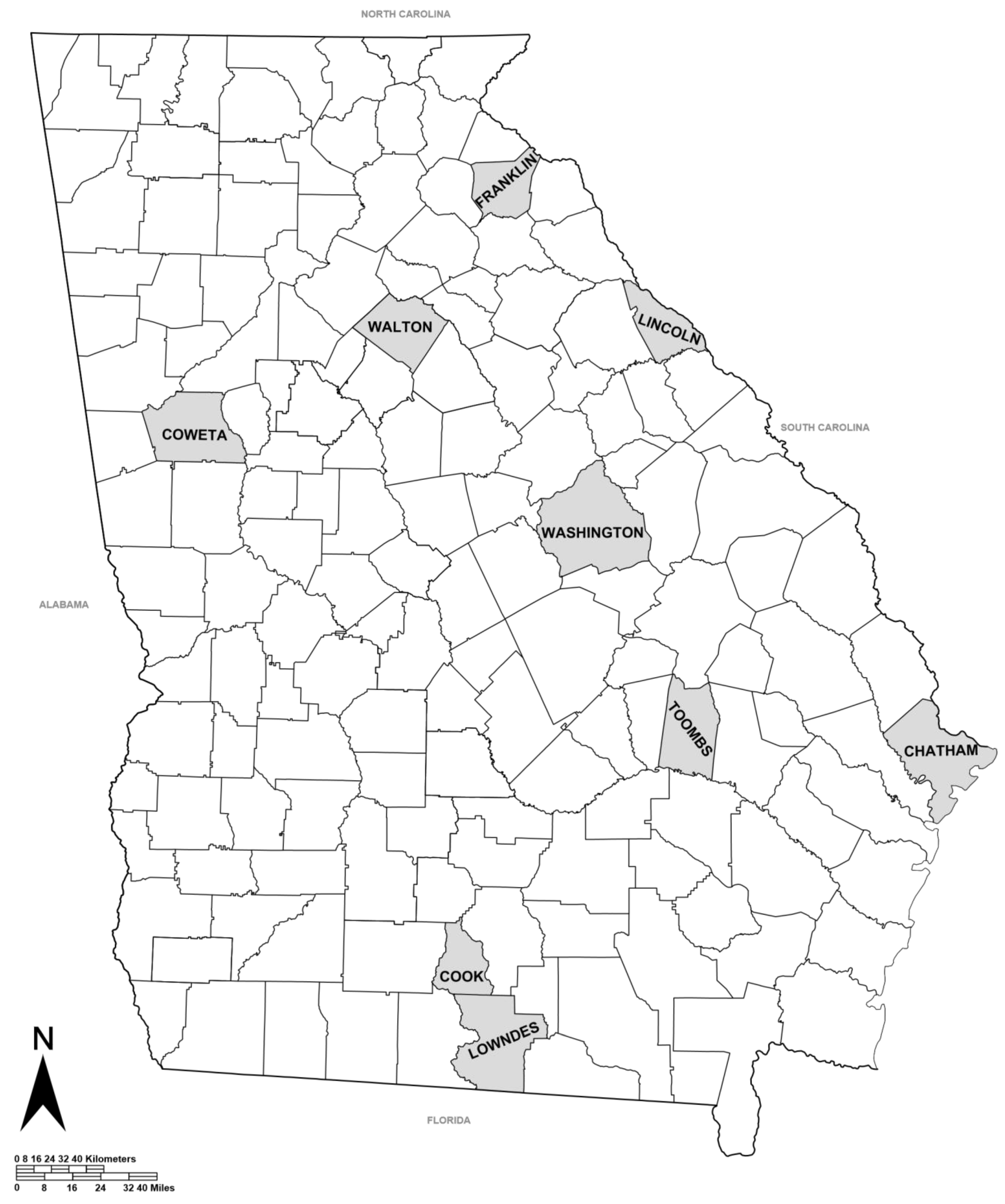
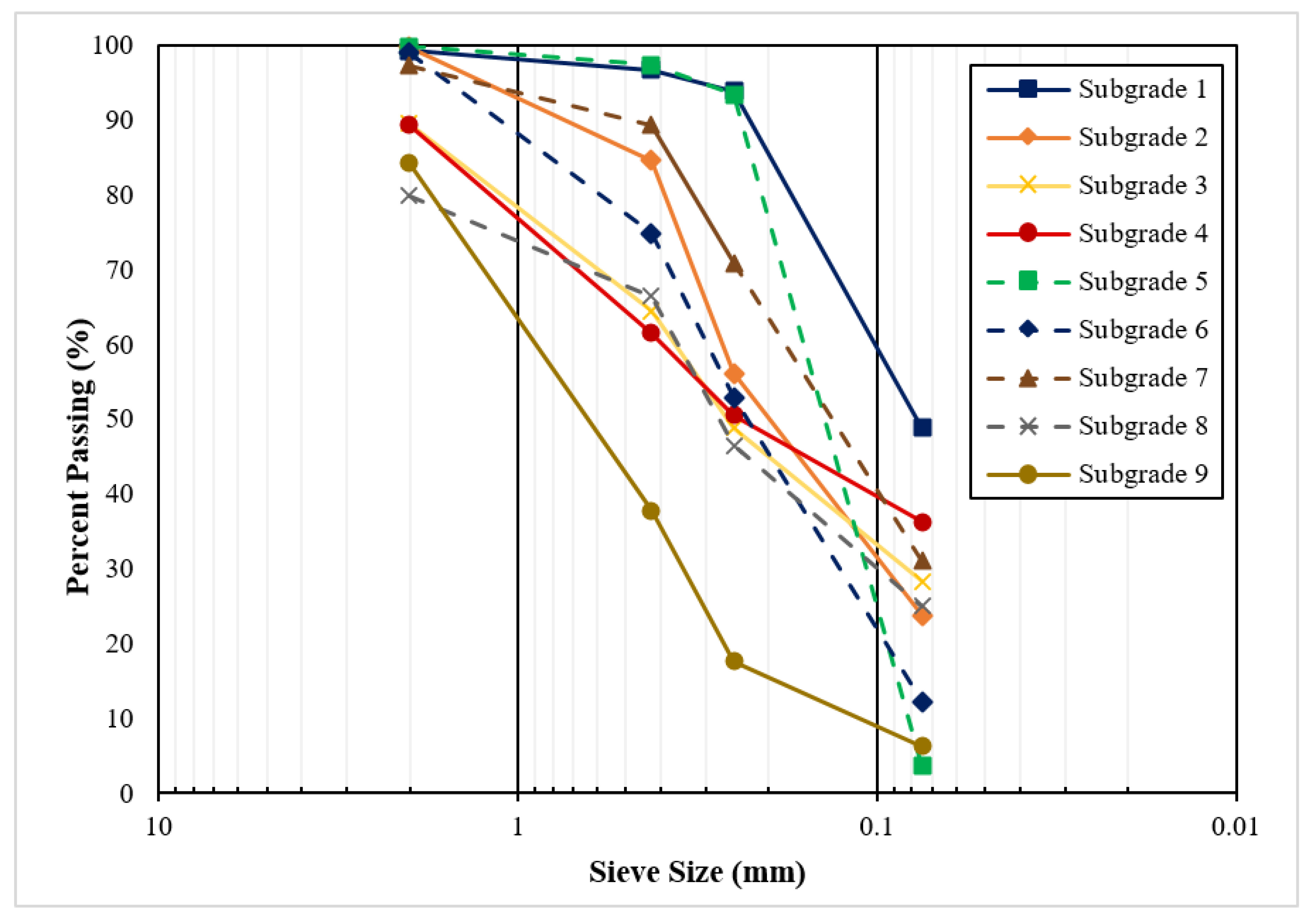
In this study, laboratory test data from a previous study were utilized to establish a correlation between M_R and a number of influential variables [5]. The soils tested in the study were recovered from nine borrow pits located across the state of Georgia (Figure 1). These soils were selected by GDOT as being representative of materials used in subgrade construction in Georgia. As seen in

Table 1. Subgrade sources and properties [4].

Subgrade No.	Location (County)	Percent Passing (%)				% Clay	% Volume Change	Max. Dry Density (pcf)	Opt. Moisture Content (%)	LL (%)	PI (%)	USCS Soil Class	AASHTO Soil Class	Number of Successfully Tested Specimens
		#10	#40	#60	#200
1	Lincoln	99	96.8	94	48.9	40.7	24.5	93.4	23.5	39.9	8.6	SC	A-4	3
2	Washington	100	84.6	56	23.8	20.6	4.7	117.8	11.0	23	6.6	SM	A-2-4	2
3	Coweta	90	64.6	49	28.3	24	12.2	105.3	16.7	42.5	11	SC	A-2-7	3
4	Walton	89	61.5	51	36.3	28.3	4.0	104.8	16.8	40.5	12.7	SC	A-7-6	3
5	Chatham	100	97.4	94	3.6	1.8	3.6	97.4	12.7	0.0	0.0	SM	A-2-4	1
6	Lowndes	99	74.9	53	12.2	4.5	0.0	113.1	4.7	0.0	0.0	SP	A-2-4	2
7	Franklin	97	89.4	71	31.1	19.6	5.2	105.1	22.6	39.3	9.8	SC	A-2-4	1
8	Cook	80	66.4	47	25	18.4	0.6	113.1	9.9	0.0	0.0	SM	A-2-4	1
9	Toombs	84	37.8	18	6.2	4.6	1.1	119.3	11.9	0.0	0.0	SP	A-1-b	2

, all nine soils were classified as sands (SC, SM, or SP). The physical properties were determined based on AASHTO T-89 (Liquid Limit Test) [22] and AASHTO T-90 (Plastic Limit Test) [23]. The standard proctor test was conducted in accordance with AASHTO T-99 to obtain optimum moisture content and maximum dry density [24]. The soils were also classified according to the Unified Soil Classification System (USCS) and AASHTO Soil Classification System. The particle size distributions for each of the nine subgrade soils are presented in Figure 2.

AASHTO T 307-99 was followed to determine the laboratory resilient modulus of the soil samples, using repeated load testing (RLT) equipment. The testing conditions were selected to simulate traffic wheel loading at a dynamic cyclic load rate of 0.1 s for every rest period of 0.9 s. The testing sequence included a range of deviator stresses for a set of confining pressures. For each confining pressure, the resilient modulus was determined by averaging the resilient deformation for the last five deviator stress cycles. Based on the averages from using this method, a design resilient modulus was determined to represent the expected subgrade condition in the pavement structure.

Three replicates for each of the nine subgrade soils were prepared for a total of 27 test specimens. However, 9 of specimens were broken during the test. As a result, the data used in this study were based on 18 successfully tested specimens. Note that 15 stress states were tested for each specimen, resulting in 270 samples. The cylindrical test specimens were fabricated to be 100 mm in diameter by 200 mm high and were compacted by using impact methods. To remove the effect of initial permanent deformation, the specimens were conditioned at a deviator stress of 4 psi and confining pressure of 6 psi for 500 load repetitions. Then, 100 load repetitions were applied to the specimens for a loading sequence that ranged from 2 to 6 psi for the confining stress and from 2 to 10 psi for the deviator stress. The mean deviator stress and mean recovered strain were then used to calculate the mean resilient modulus at each stress state.

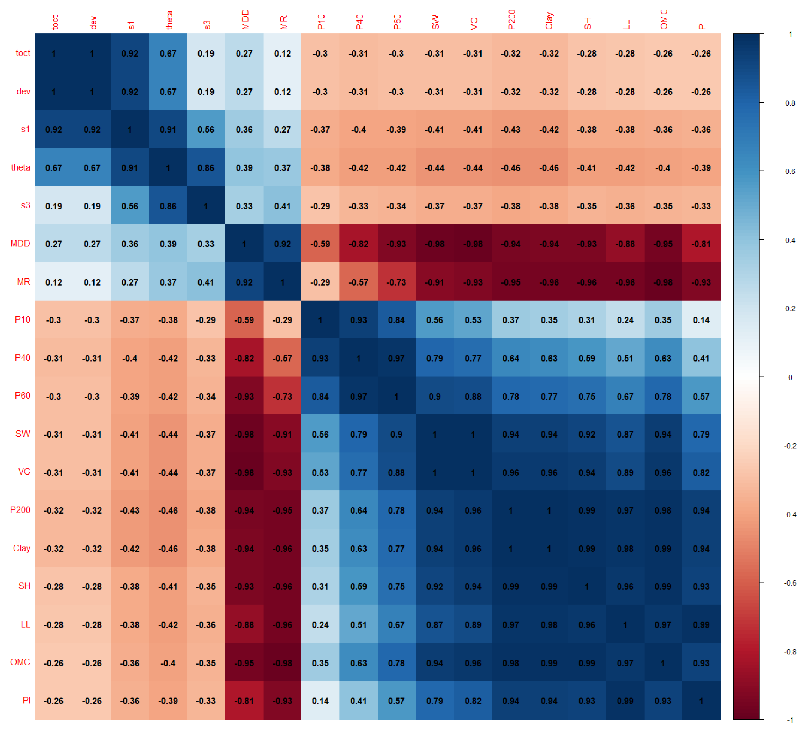
For modeling purposes, the M_R test results and the soil properties test data routinely collected by GDOT were pooled together to form a dataset. The variables included in the dataset are shown in

Table 2. Summary of variables.

Variable	Description	Unit	Min	Max	Mean
P10	Percentage of sample material (by weight) passing through the No. 10 sieve.	%	79.9	99.9	93.2
P40	Percentage of sample material (by weight) passing through the No. 40 sieve.	%	37.8	97.4	73.1
P60	Percentage of sample material (by weight) passing through the No. 60 sieve.	%	17.6	93.8	58
P200	Percentage of sample material (by weight) passing through the No. 200 sieve.	%	3.6	48.9	26.9
Clay	Percentage of clay (by weight) of the soil sample.	%	1.8	40.7	21.0
VC	Percentage of volume change of the soil sample as the material passes from a dry to soaked state.	%	0.0	24.5	7.8
SW	Percentage of soil swell	%	0.0	20.5	6.4
SH	Percentage of soil shrinkage	%	0.0	4.0	1.6
MDD	Maximum Dry Density is the dry density of the soil sample at the peak of its parabolic relationship with moisture content.	lbs./ft3	93.4	119.3	107.0
OMC	Optimum Moisture Content is the moisture percentage (by weight) of the soil sample at its MDD.	%	4.7	23.5	15.1
LL	Liquid Limit	%	0.0	42.5	25.2
PI	Plastic Index	%	0.0	12.7	6.7
s1	Principal vertical stress at which testing was conducted	lbs./in2	4.0	16.0	10.0
s3	Confining pressure at which testing was conducted	lbs./in2	2.0	6.0	4.0
dev	Deviator Stress $dev=s_1-s_3$	lbs./in2	2.0	10.0	6.0
theta	$theta=s1+2\left(s3\right)$	lbs./in2	8.0	28.0	18.0
toct	$toct=\frac{1}{3}\sqrt{{\left(s1-s3\right)}^2+{\left(s3-s1\right)}^2}$	lbs./in2	0.9	4.7	2.8
MR	Resilient Modulus	lbs./in2	3174	25,887	11,400

. The correlation matrix of these variables is presented in Figure 3.

As shown in Figure 3, t_oct and dev are perfectly correlated according to their definitions. The correlation coefficient between SW and VC and between clay and P200 are nearly 1.0 as well.

4. Decision Tree and Ensemble Methods

Decision trees partition the feature space into a set of distinct and non-overlapping regions, and then they fit a simple model (such as a constant) in each region. It is computationally infeasible to consider every possible partition of the feature space due to curse of dimensionality. Instead, a “top-down” and “greedy” approach, known as recursive binary splitting, has been generally used together with cost complexity pruning.

The classification and regression tree (CART) is a popular one proposed by Breiman et al. [25] to construct decision trees. The major advantages of trees are their interpretability and ease in handling qualitative predictors without creating dummy variables. However, the major issue with trees is their high variance, meaning a small change in the data could result in a very different tree structure. The main reason for this instability lies in the hierarchical nature of the tree’s construction process: the effect of an error in the top split is propagated down to all of the splits below it [26]. Other major limitations of trees include the lack of smoothness of the prediction surface and difficulty in capturing the additive structure. In solving most of these issues, tree-based ensemble methods have been developed and refined over time. Tree ensemble methods are scalable to practically large dataset. They are invariant to scaling of inputs and can learn higher-order interaction among features.

There are two major categories of ensemble methods: parallel ensemble and sequential ensemble. In parallel ensemble, each tree model is built independently, typically with a bootstrapped sample. The main idea is to combine many of individual trees to reduce variance. For example, for regression problems, the predictions of individual trees in an ensemble are averaged to produce the final prediction, which can significantly reduce variance if the samples are independently drawn from the underlying population. On the other hand, in sequential ensemble, tree models are generated sequentially with the later trees to correct the errors made by previous trees in sequence. In practice, a shrinkage factor (also referred to as learning rate) is often applied to prevent overfitting. In the inference stage, the trees are summed to produce the final prediction.

The most popular and well-known model of parallel ensemble is Random Forest (RF) [27], while for the sequential ensemble, variants of gradient boosting methods have been developed with the eXtreme Gradient Boosting (XGBoost) [28] being one of the most popular methods. In RF, bootstrapped samples are used to fit individual trees. Instead of selecting a node-splitting feature from the full set of predictors, a random subset of predictors is chosen, and those predictors are the candidates for node splitting, to reduce correlation among trees. In XGBoost, gradient boosting is extended to the second order and a novel explicit penalty term on tree complexity is added to the objective function. XGBoost has achieved state-of-the-art results on many machine learning challenges and is capable of scaling beyond billions of examples by using far fewer resources. Both methods have recently been applied across different domains [29,30,31].

In this study, we explored the utility of Decision Tree, RF, and XGBoost methods in modeling and predicting the subgrade resilient modulus of subgrade materials. The tree-based models developed were further compared with a traditional Multiple Linear Regression (MLR) model fitted using the same training dataset to demonstrate the superiority of the tree ensemble methods.

5. Model Development and Evaluation

In machine learning applications, data are typically split into training and testing datasets; the training dataset is used for model development, while the test dataset for the final model test. Training dataset is normally further divided into multiple folds (k folds) for cross-validation and hyperparameter tuning. The cross-validation is especially necessary for small datasets, which is our case. Our dataset for this study contains 270 resilient modulus test results on nine sandy subgrade soils. The dataset was randomly divided into training and testing datasets with an 80–20 split. The basic M_R statistics of the training and testing datasets are provided in

Table 3. Summary of statistics for M_R.

	Training Dataset	Testing Dataset	Total Dataset
Number of Observations	216	54	270
Average MR	11,277 psi	11,894 psi	11,400 psi
Standard Deviation	5392 psi	5967 psi	5505 psi

, showing similar distributions.

All models were developed by using the training dataset, and their performances were evaluated and compared by using the test dataset. The development of each model type and the corresponding results are presented and discussed subsequently.

5.1. Regression Tree Model

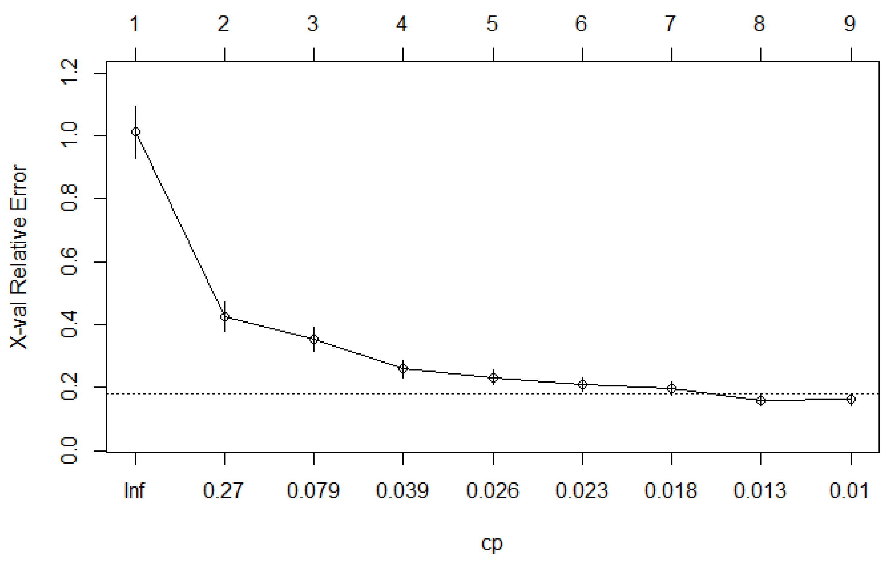
For developing the regression tree model, the rpart package [32] was used. As part of the package, multiple cost complexities were evaluated with cross-validation. Figure 4 shows the cross-validation error plotted with respect to the cost complexity factor, as well as the tree size.

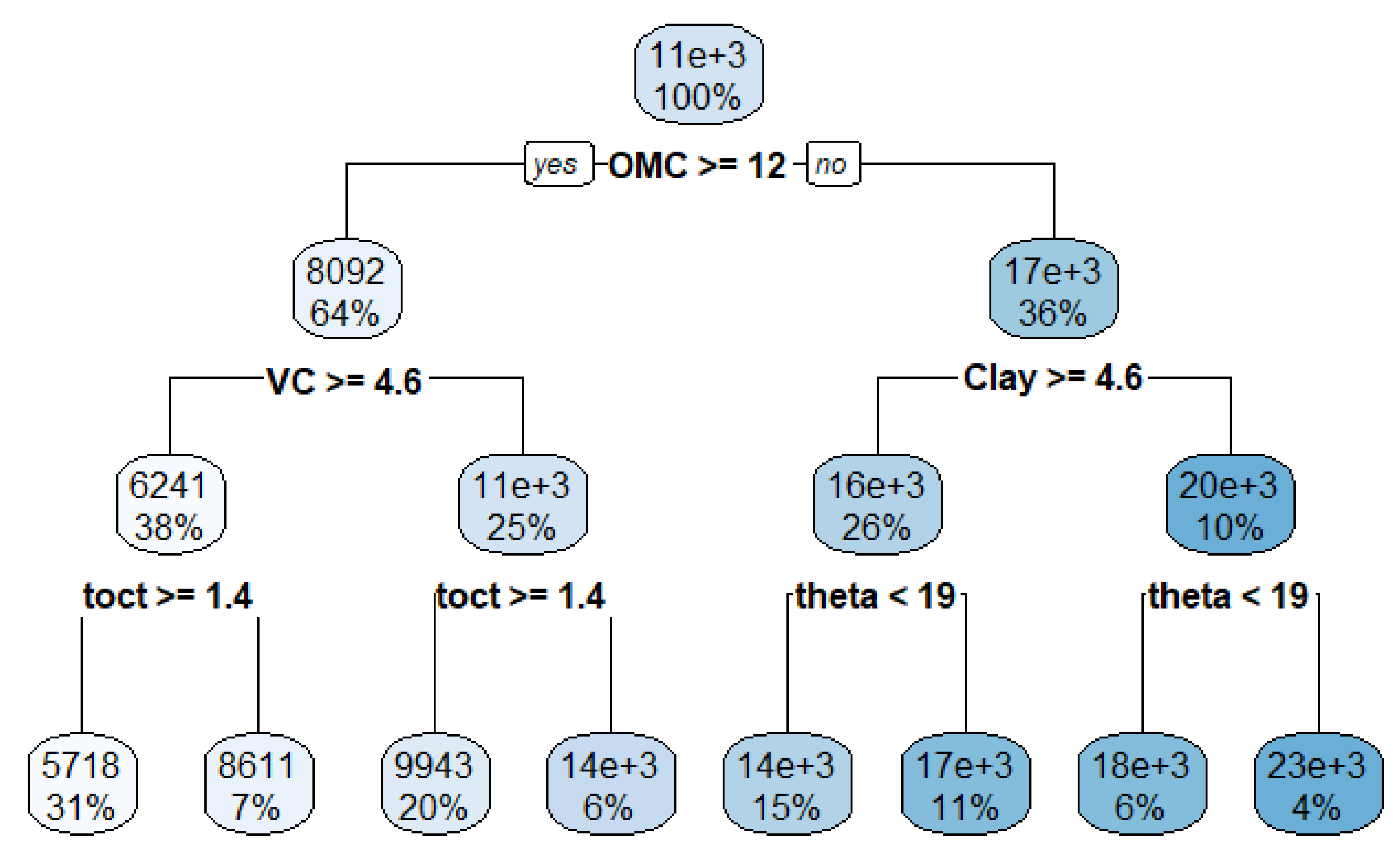
As indicated in Figure 4, the tree with eight terminal nodes has the minimum cost complexity factor, and it is selected and plotted in Figure 5.

As shown in Figure 5, for M_R prediction, the most important variable (root node) is the optimum moisture content (OMC), followed by the clay content (Clay) and volume change percentage (VC). Moreover, t_oct and theta are also important variables in explaining the variance in M_R.

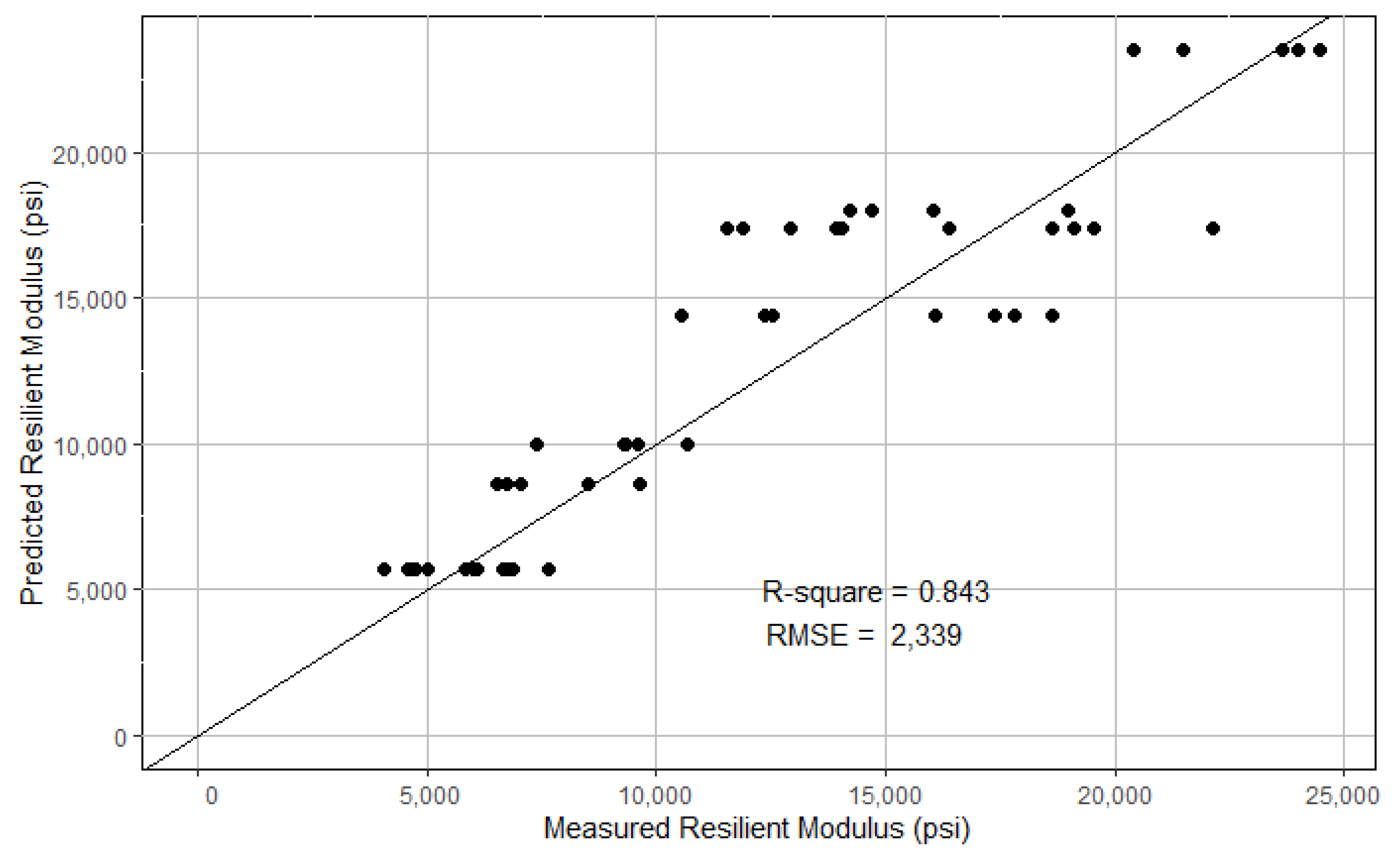
The model developed by using the training dataset was evaluated on the testing dataset. For visualization, the model-predicted M_R and the lab-measured M_R are plotted against the equality line, as shown in Figure 6. The Root Mean Squared Error (RMSE) was computed to be 2339 lbs./in². The R² was computed to be 0.843 with respect to the equality line.

5.2. Random Forest Model

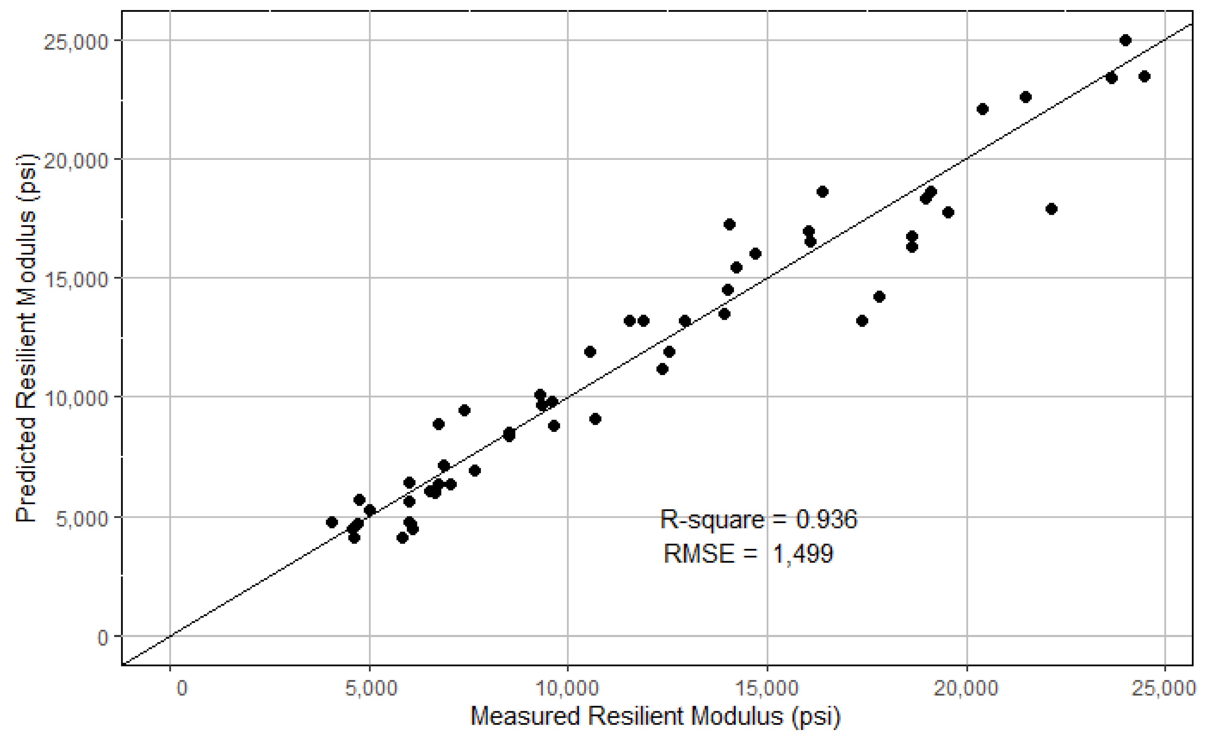
The randomForest package [33] was used to develop the RF model. The hyperparameters were optimized through a cross-validation-based grid search method adopted in the caret package [34]. As a result, the number of trees (ntree) and the number of variables randomly sampled as candidates at each split (mtry) were selected to be 50 and 10, respectively. Given the relatively small dataset, the minimum size of terminal nodes was chosen to be 5. The final model was evaluated on the test dataset, and the model-predicted M_R and the lab-measured M_R are plotted in Figure 7. The RMSE and R² were computed to be 1499 and 0.936, respectively.

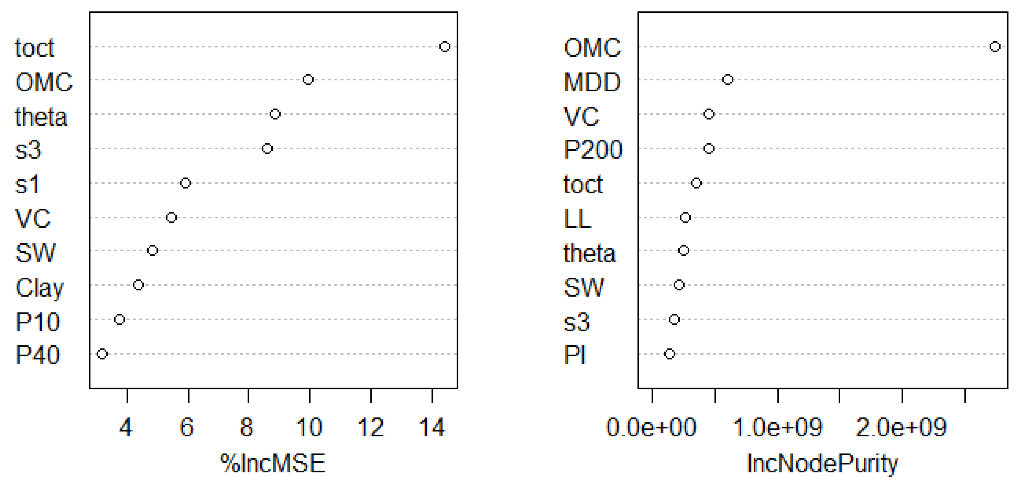
Tree ensemble models have a natural way of evaluating variable importance. Two typically used metrics in random forest are percent increment in mean squared errors (%IncMSE) and increment in node purity (IncNodePurity). The former indicates how much error increases if a subject variable is removed, while the latter measures how much node purity (in terms of Gini impurity index) increases if a subject variable is removed. The relative importance plots are shown in Figure 8. As indicated, the two lists of top 10 important variables are not completely agreeable. However, both importance metrics chose OMC, t_oct, theta, VC, SW, and s3 among the top 10 most importance variables. Clay was selected by the %incMSE metric, while P200 was selected by the IncNodePurity metric, noting that these two variables are highly correlated (see Figure 3).

5.3. XGBoost Model

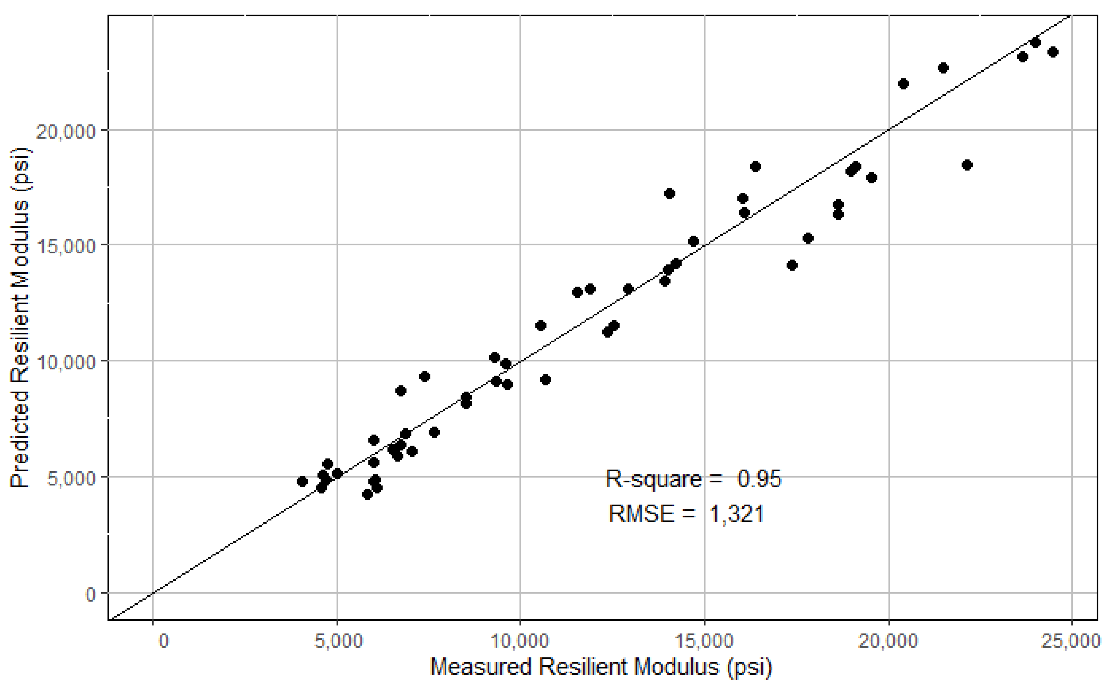
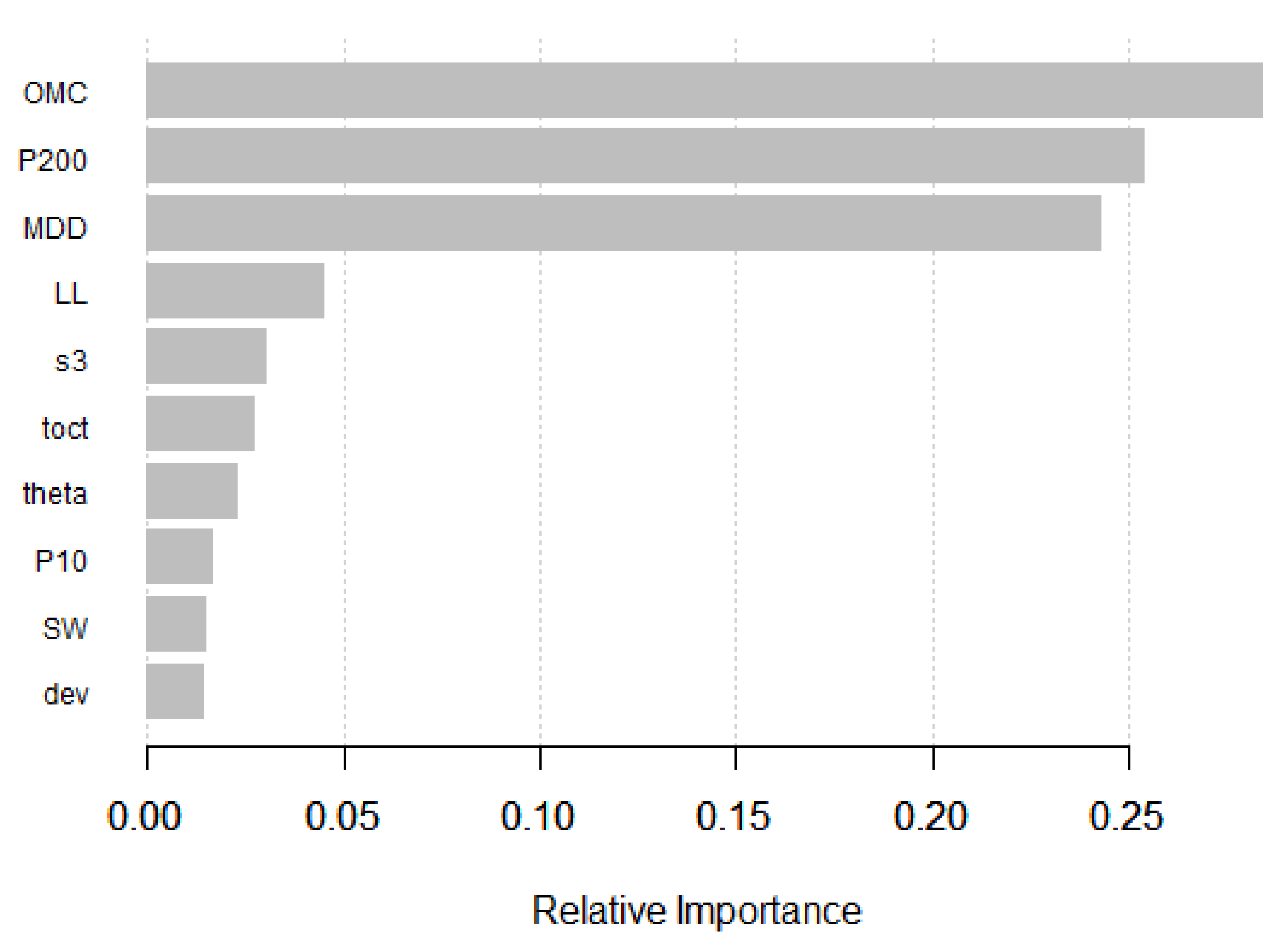
The XGBoost model was trained by using the xgboost package [35]. Similar to the RF model development, the cross-validation based grid search method was applied to find the best hyperparameters: the number of boosting iterations (nrounds) = 50, maximum depth of trees (max_depth) = 4, learning rate (eta) = 0.1, the subsample ratio of columns (colsample_bytree) = 1, minimum sum of instance weight needed in a child (min_child_weight) = 0.5, and the subsample ratio of the training instances (subsample) = 0.8. Figure 9 shows the model-predicted M_R versus the lab-measured M_R. The RMSE and R² were computed to be 1321 and 0.95, respectively. The relative importance of the top 10 variables is shown in Figure 10, with the top three variables being OMC, P200, and MDD.

5.4. Multiple Linear Regression Model

For comparison purposes, a traditional MLR model was fitted with the same training dataset used for developing the tree-based models. The estimation results of the MLR model are summarized in

Table 4. Model Estimation Results (MLR Model).

Variable	Estimate	SE	T-Value	P-Value	Sig.
(Intercept)	13147.86	3682.27	3.571	0.000	***
P200	155.82	20.53	7.589	0.000	***
MDD	77.06	29.05	2.652	0.009	**
OMC	−881.82	56.52	−15.602	0.000	***
PI	−277.45	47.22	−5.876	0.000	***
theta	209.76	30.07	6.977	0.000	***
toct	−1004.75	127.68	−7.869	0.000	***
	R2 = 0.839
	Residual Standard Error = 2191
	F statistic = 182.1 (p-value < 2.2 × 10−16)

Sig.: *** 0.001; ** 0.01.

, revealing a fairly good fit to the training dataset. By referencing the absolute t-value in Table 4, the most significant variable is OMC, followed by t_oct, P200, theta, PI, and MDD. The signs of the estimates indicate that increase in OMC, t_oct and PI would result in a decrease in M_R while increase in P200, theta, and MDD would result in an increase in M_R.

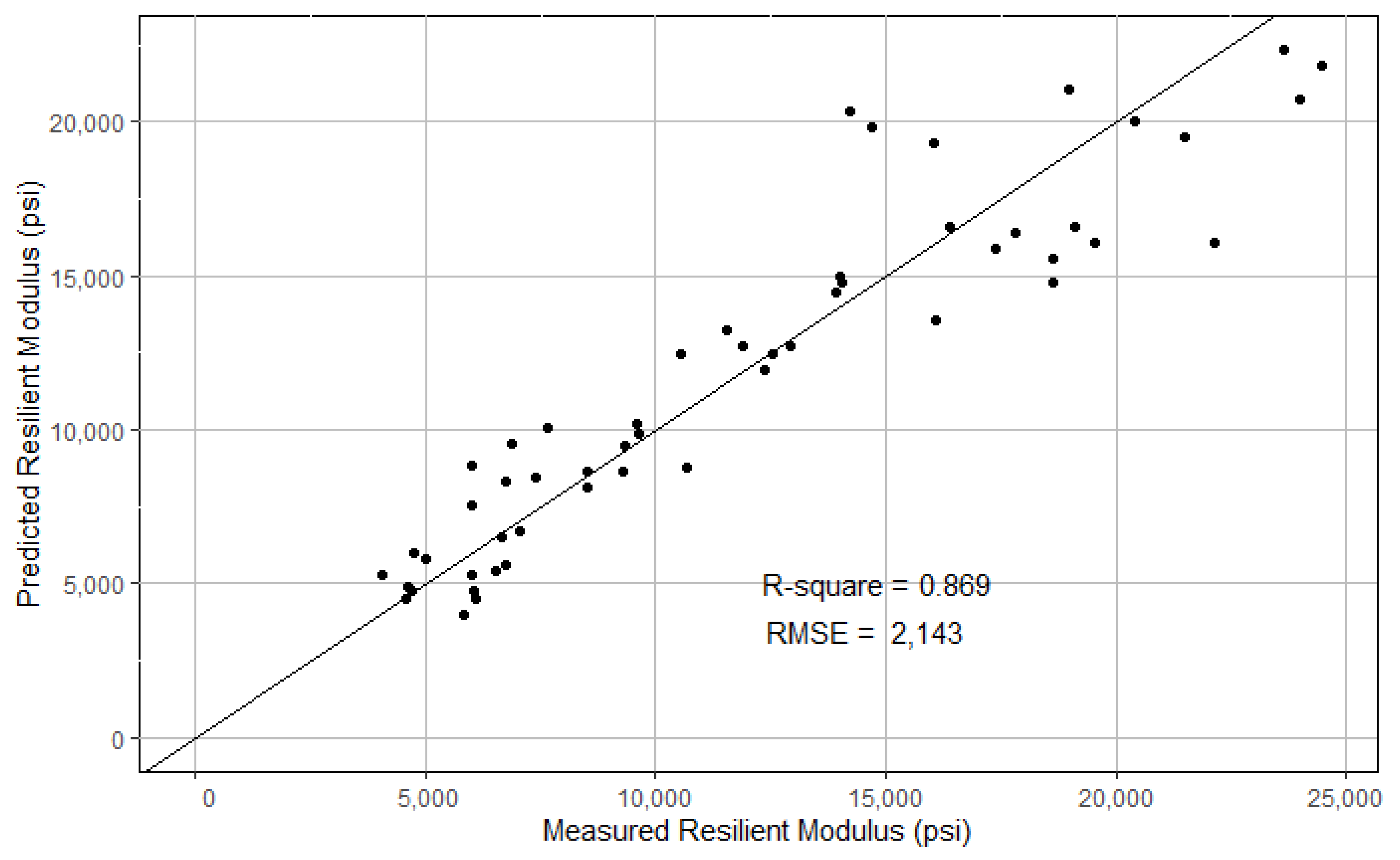
The MLR model was further evaluated on the same test dataset. The model-predicted M_R and the lab-measured M_R are plotted in Figure 11. The RMSE and R² were computed to be 2143 and 0.869, respectively.

6. Model Comparison

For direct comparison of all four models presented previously, the RMSE and R² are compiled in

Table 5. Comparison of model performance on the test dataset.

	MLR	Regression Tree	RF	XGBoost
R2	0.869	0.843	0.936	0.950
RMSE	2143	2339	1499	1321

, and the top five most important variables are summarized in

Table 6. Comparison of variable importance across models.

Rank	MLR (1)	Regression Tree (2)	RF (3)	XGBoost (4)
1	OMC	OMC	OMC	OMC
2	toct	VC	MDD	P200
3	P200	Clay	VC	MDD
4	theta	toct	P200	LL
5	PI	theta	toct	s3

Notes: ⁽¹⁾ ranking is based on the absolute t value, ⁽²⁾ ranking is based on the hierarchical order in the tree, ⁽³⁾ ranking is based on the increment in node purity, and ⁽⁴⁾ ranking is based on the relative importance.

. The MLR model and the Regression Tree model share similar performance in terms of RMSE and R². The MLR model slightly outperformed the Regression Tree model, while the latter has a much simpler model structure (see Figure 5). As expected, both tree ensemble methods (RF and XGBoost) outperformed the MLR and Regression Tree models, with significantly improved performance, evidenced by much lower RMSE and higher R².

As indicated in Table 6, the top single most important variable (i.e., OMC) is same across all four models, and many other top variables are shared across the models. For example, among the top five most importance variables, t_oct appeared in the MLR, Regression Tree, and RF models, while P200 showed up in the MLR, RF, and XGBoost models, noting that Clay is the third most importance variable for the Regression Tree, which has nearly perfect correlation with P200. The variation in variable importance and ranking across models is likely due to the difference in model structures and algorithms used for model training or fitting. For example, the MLR model is constrained by its linear-in-parameter assumption, while tree-based models are nonlinear in nature and more flexible than the MLR.

7. Conclusions

M_R is a critical input parameter for the MEPDG. As many state transportation agencies have started adopting the MEPDG, there has been an invested effort to develop reliable models that are capable of predicting M_R from routinely measured soil properties. As such, movement towards full adoption of the MEPDG can be achieved with the least disruption to a state’s existing procedures.

In this paper, modern machine learning methods, such as tree ensembles, were explored in modeling and predicting M_R. The laboratory test data in Georgia were utilized for model development and evaluation. In maximizing the limited data resource, a cross-validation procedure was applied for model training and hyperparameter fine-tuning. Two powerful tree ensemble models, i.e., RF and XGBoost, were developed and compared with a Regression Tree model and a traditional MLR model, fitted using the same training dataset. All four models were evaluated on the same test dataset. The results revealed that both tree ensemble models (RF and XGBoost) significantly outperformed the Regression Tree and MLR models, and the XGBoost model produced the best performance.

In conclusion, single tree models, although flexible, are subject to high variance. They are generally considered weak leaners with limited capacity, while tree ensembles are able to leverage a collection of weak leaners to significantly improve prediction accuracy with reduced variance. The tree ensemble models, endowed with powerful structure, offer ample capacity to learn from various heterogeneous data sources. Unlike traditional MLR models, which impose restrictive assumptions, such as linearity in parameters, error normality, and homogeneity, tree ensemble models are much more flexible and versatile, especially in learning complex nonlinear relationships in high-dimensional feature spaces.

References

- ARA Inc. Guide for Mechanistic-Empirical Design of New and Rehabilitated Pavement Structures; ARA Inc.: Champaign, IL, USA, 2004. [Google Scholar]
- Georgia Department of Transportation. Georgia Department of Transportation Pavement Design Manual; Georgia Department of Transportation: Forest Park, GA, USA, 2019. [Google Scholar]
- Von Quintus, H.L.; Darter, M.I.; Bhattacharya, B.; Titus-Glover, L. Implementation and Calibration of the MEPDG in Georgia; Georgia Department of Transportation: Forest Park, GA, USA, 2016. [Google Scholar]
- AASHTO. AASHTO T 307-99: Standard Method of Test for Determining the Resilient Modulus of Soils and Aggregate Materials; AASHTO: Washington, DC, USA, 2003. [Google Scholar]
- Kim, S.H. Measurements of Dynamic and Resilient Moduli of Roadway Test Sites; Georgia Department of Transportation: Forest Park, GA, USA, 2013. [Google Scholar]
- Malla, R.B.; Joshi, S. Subgrade resilient modulus prediction models for coarse and fine-grained soils based on long-term pavement performance data. Int. J. Pavement Eng. 2008, 9, 431–444. [Google Scholar] [CrossRef]
- Yau, A.; Von Quintus, H.L. Study of LTPP Laboratory Resilient Modulus Test Data and Response Characteristics; No. FHWA-RD-02-051; Federal Highway Administration: McLean, VA, USA, 2002. [Google Scholar]
- Puppala, A.J. Estimating Stiffness of Subgrade and Unbound Materials for Pavement Design; NCHRP Synthesis 382; Transportation Research Board: Washington, DC, USA, 2008; p. 132. [Google Scholar] [CrossRef]
- Huang, Y.H. Pavement Analysis and Design; Pearson Education, Inc.: Upper Saddle River, NJ, USA, 2004. [Google Scholar]
- Kim, D.; Kim, J.R. Resilient behavior of compacted subgrade soils under the repeated triaxial test. Constr. Build. Mater. 2007, 21, 1470–1479. [Google Scholar] [CrossRef]
- Kamal, M.; Dawson, A.; Farouki, O.; Hughes, D.; Sha’at, A. Field and laboratory evaluation of the mechanical behavior of unbound granular materials in pavements. Transp. Res. Rec. 1993, 1406, 88–97. [Google Scholar]
- Elliott, R.P. Selection of subgrade modulus for AASHTO flexible pavement design. Transp. Res. Rec. 1992, 1354, 39–44. [Google Scholar]
- Drumm, E.; Boateng-Poku, Y.; Johnson Pierce, T. Estimation of subgrade resilient modulus from standard tests. J. Geotech. Eng. 1990, 116, 774–789. [Google Scholar] [CrossRef]
- Brown, S.; Pell, P. An experimental investigation of the stresses, strains and deflections in a layered pavement structure subjected to dynamic loads. In Proceedings of the International Conference on the Structural Design of Asphalt Pavements, Ann Arbor, MI, USA, 7–11 August 1967. [Google Scholar]
- Hicks, R.G.; Monismith, C.L. Factors influencing the resilient response of granular materials. Highw. Res. Rec. 1971, 345, 15–31. [Google Scholar]
- Siekmeier, J.; Pinta, C.; Merth, S.; Jensen, J.; Davich, P.; Camargo, F.; Beyer, M. Using the Dynamic Cone Penetrometer and Light Weight Deflectometer for Construction Quality Assurance; Minnesota Department of Transportation: St Paul, MN, USA, 2009.
- Hossain, M.S. Estimation of subgrade resilient modulus for Virginia soil. Transp. Res. Rec. 2009, 2101, 98–109. [Google Scholar] [CrossRef]
- Richter, C.A. Seasonal Variations in the Moduli of Unbound Pavement Layers; No. FHWA-HRT-04-079; United States Federal Highway Administration: McLean, VA, USA, 2006.
- Jin, M.S.; Lee, K.W.; Kovacs, W.D. Seasonal Variation of Resilient Modulus of Subgrade Soils. J. Transp. Eng. 1994, 120, 603–616. [Google Scholar] [CrossRef]
- Lekarp, F.; Isacsson, U.; Dawson, A. State of the art. Part I: Resilient response of unbound aggregates. J. Transp. Eng. 2000, 126, 66–75. [Google Scholar] [CrossRef] [Green Version]
- Kessler, K. Use of DCP (dynamic cone penetrometer) and LWD (light weight deflectometer) for QC/QA on subgrade and aggregate base. In GeoHunan International Conference; American Society of Civil Engineers: Reston, VA, USA, 2009; pp. 62–67. [Google Scholar] [CrossRef]
- AASHTO T 89. Standard Method of Test for Determining the Liquid Limit of Soils; American Association of State Highway and Transportation Officials: Washington, DC, USA, 2006. [Google Scholar]
- AASHTO T 90. Standard Method of Test for Determining the Plastic Limit and Plasticity Index of Soils; American Association of State Highway and Transportation Officials: Washington, DC, USA, 2006. [Google Scholar]
- AASHTO T 99. Standard Method of Test for Moisture Density Relations of Soils Using a 2.5 kg Rammer and a 305 mm Drop; American Association of State Highway and Transportation Officials: Washington, DC, USA, 2007. [Google Scholar]
- Breiman, L.; Friedman, J.; Stone, C.J.; Olshen, R.A. Classification and Regression Trees; CRC Press: Boca Raton, FL, USA, 1984. [Google Scholar] [CrossRef]
- Hastie, T.; Tibshirani, R.; Friedman, J. The Elements of Statistical Learning: Data Mining, Inference, and Prediction, 2nd ed.; Springer Series in Statistics; Springer: New York, NY, USA, 2009. [Google Scholar]
- Breiman, L. Random Forests. Mach. Learn. 2001, 45, 5–32. [Google Scholar] [CrossRef] [Green Version]
- Chen, T.; Guestrin, C. Xgboost: A scalable tree boosting system. In Proceedings of the 22nd ACM SIGKDD International Conference on Knowledge Discovery and Data Mining, San Francisco, CA, USA, 13–17 August 2016; pp. 785–794. [Google Scholar]
- Salehi, I.H.; Christian, J.; Kim, S.; Sutter, L.; Durham, S.; Yang, J.; Vickery, C.G. Use of Random Forest Model to Identify the Relationships Among Vegetative Species, Salt Marsh Soil Properties, and Interstitial Water along the Atlantic Coast of Georgia. Infrastructures 2021, 6, 70. [Google Scholar] [CrossRef]
- Salehi, I.H.; Kim, S.; Sutter, L.; Christian, J.; Durham, S.; Yang, J. Machine Learning Approach to Identify the Relationship Between Heavy Metals and Soil Parameters in Salt Marshes. Int. J. Environ. Sci. Nat. Resour. 2021, 27, 556224. [Google Scholar]
- Morris, C.; Yang, J. Understanding Multi-Vehicle Collision Patterns on Freeways—A Machine Learning Approach. Infrastructures 2020, 5, 62. [Google Scholar] [CrossRef]
- Therneau, T.; Atkinson, B. Rpart: Recursive Partitioning and Regression Trees; R Package Version 4.1-15; 2019; Available online: https://CRAN.R-project.org/package=rpart (accessed on 5 May 2021).
- Liaw, A.; Wiener, M. Classification and Regression by randomForest. R News 2002, 2, 18–22. [Google Scholar]
- Kuhn, M. Caret: Classification and Regression Training; R Package Version 6.0-86; 2020; Available online: https://CRAN.R-project.org/package=caret (accessed on 5 May 2021).
- Chen, T.; He, T.; Benesty, M.; Khotilovich, V.; Tang, Y.; Cho, H.; Chen, K.; Mitchell, R.; Cano, I.; Zhou, T.; et al. xgboost: Extreme Gradient Boosting; R Package Version 1.2.0.1; 2020; Available online: https://CRAN.R-project.org/package=xgboost (accessed on 5 May 2021).
Figure 1.
Subgrade borrow pit locations.
Figure 2.
Subgrade gradation [4].
Figure 3.
Correlation matrix of variables. (Note: the correlation coefficient values only show up to two decimal points.)
Figure 4.
Cross-validation error versus cost complexity factor.