
Risk Assessment of Terrestrial Transportation Infrastructures Exposed to Extreme Events

 , , and
Abstract
:1. Introduction
1.1. Risk Assessment of Terrestrial Transportation Infrastructures in the Literature
1.2. Scope of the Paper
- Preparation: by improving risk estimation and prediction and by developing better monitoring and decision tools;
- Response and recovery: by optimizing emergency plans and real-time communication with operators and end users;
- Mitigation: by introducing new construction systems and smart materials and by assessing consequences of different scenarios and mitigation solutions for selection of the optimal mitigation strategy.
- Different levels of detail (regarding accuracy and complexity) and analysis scale (e.g., at asset level, within a transportation link or at network level);
- Different types of infrastructure assets;
- Natural extreme events (with focus on weather-related hazards) and unintentional human-made extreme events; (i.e., potentially disastrous events or disorders caused by human activity. Human errors [41] related to technical human activities are not included);
- Assessment of structural damage and loss of mobility. The safety of the users is not considered directly, i.e., cases where road or railway users are directly injured by an extreme event are not considered, and the focus is on the infrastructure assets.
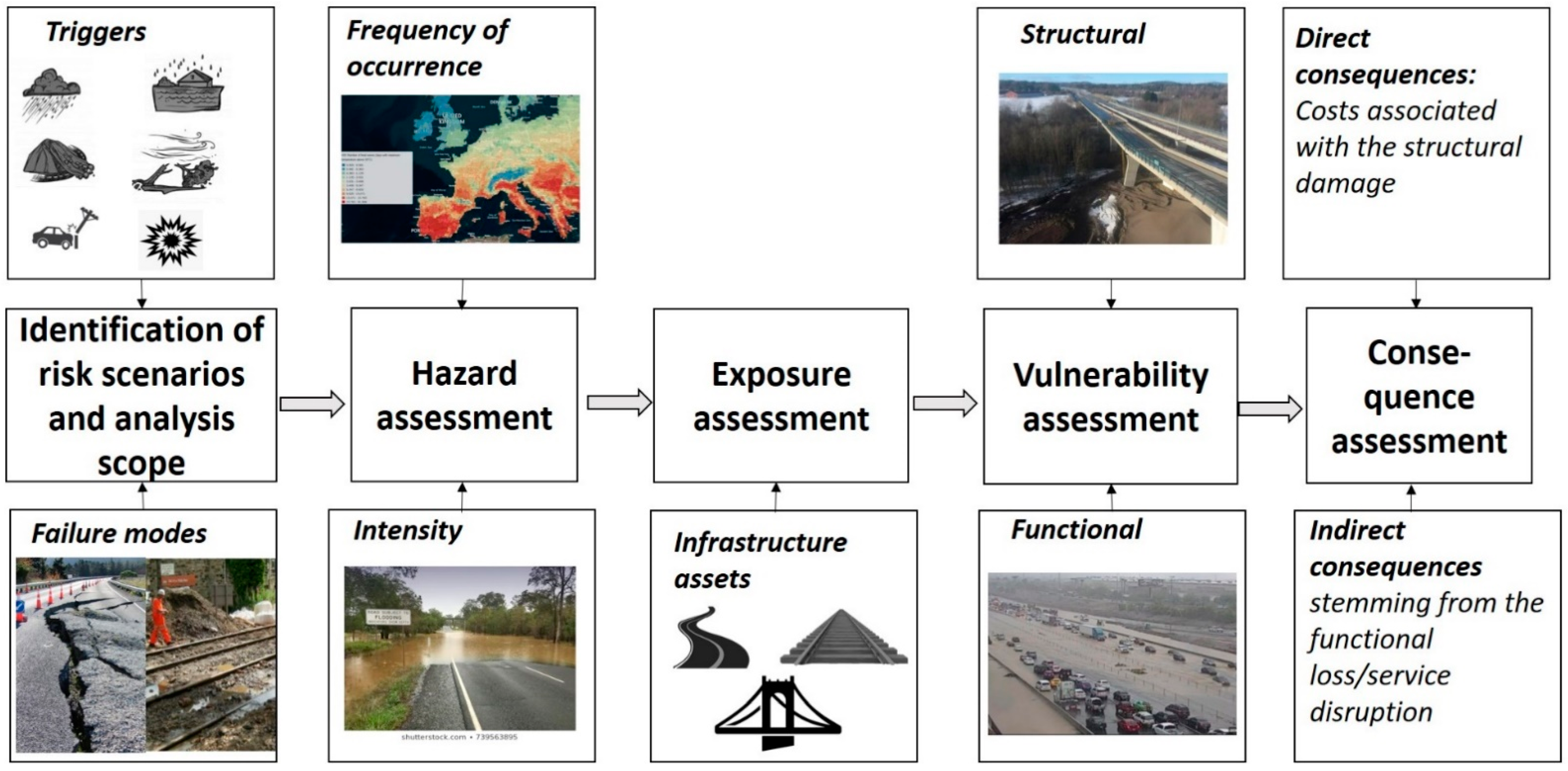
2. Risk Assessment of Terrestrial Transportation Systems—Conceptualization of the Assessment Steps
- What can cause harm? (Potential threats and adverse events are identified.)
- How often may the identified adverse event occur? (What is the frequency of occurrence?)
- What can go wrong? (Which are the exposed elements and what are the consequences?)
- If it goes wrong, how severe are the consequences? (The severity will depend on the robustness/resistance of the exposed elements/assets and the intensity of the hazard.)
2.1. What Can Cause Harm?
2.2. How Often May the Identified Adverse Event Occur?
- FM be the failure mode of interest. The failure mode describes the severity of structural damage and/or functional loss, due to an extreme event;
- EEi be the extreme event of interest that could trigger the failure mode;
- i represent the intensity of the extreme event EEi. The intensity is a single or a composite parameter expressing a damaging potential/action of the extreme event at asset(s) location;
- Ptemporal denote the temporal probability, e.g., annual probability expressing the occurrence probability per year.
- Structural damage to the asset, e.g., a partial failure or an asset collapse;
- Material or obstacles on the transportation line leading to service disruption, e.g., in terms of capacity reductions (e.g., a % of total capacity at an analyzed road section), speed reductions or load postings (e.g., a bridge is closed for freight traffic);
- Failure of supporting systems, where the definition of failure is contained within the detailed failure mode description;
- Dangerous driving conditions leading to restrictions, usually defined as thresholds on intensity parameters.
2.3. What Can Go Wrong?
2.3.1. Assessment of Exposure
2.3.2. Assessing the Conditional Probability of Failure Modes
- SD(FM) be the degree of structural damage of the asset(s) in the failure mode;
- SDcalc be the structural damage estimated from the damage functions.
2.3.3. Recommendations for Development/Adaptation of Structural and Functional Vulnerability Functions
- Verification of existing fragility functions to site-specific conditions, i.e., by examining if the available fragility function appropriately represents the behavior of the asset types representative of the study area.
- Adaptation of existing fragility functions to site-specific conditions, i.e., by calibrating the existing fragility function to observational data or by combining an existing fragility curve with observational data through Bayesian updating.
- Development of new fragility functions based on recommended intensity parameters in Table 3 and using one of the four main approaches to develop vulnerability models [49]:
- ○
- Judgmental: based on expert opinion or engineering judgement.
- ○
- Empirical: based on observations.
- ○
- Analytical: based on analytical or numerical solution methods.
- ○
- Hybrid approach: combining one or more of above approaches.
2.4. If It Goes Wrong: How Severe Are the Consequences?
- C(FM), Cdirect(FM) and Cindirect(FM) denote the consequences, the direct consequences and the indirect consequences respectively associated with a failure mode FM, considering the full range of plausible intensities of EEi.
- RC be the full repair and reconstruction costs of the asset.
- CS be the costs of service disruption per hour.
- D(FM) be the duration of the service disruption in hours associated with a failure mode FM.
2.4.1. Assessment of Direct Consequences
2.4.2. Assessment of Indirect Consequences
- Graph theory and topological properties of the transport network. Such approaches consider networks as a collection of vertices (or nodes) that are connected by arcs (or links) and consider the importance of different links, cascading failures and interdependencies between different networks. Graph-theoretical concepts are useful for the description of transport network characteristics and its connectivity [18].
- Understanding of the dynamic behavior exhibited on networks (e.g., traffic flow) using transportation system models, modelling demand and supply side of the transport system and travelers’ responses to disturbances and disruptions. Most risk frameworks account for traffic-related consequences using a macroscopic model with static user-equilibrium flow formulation. This traffic assignment model presents strong assumptions such as steady traffic conditions during the time of investigation, constant demand, and user’s complete knowledge of the traffic conditions. The traffic flow could be modelled, e.g., considering the traffic as a fluid and using models based on fluid dynamics equations [68]. However, it has been found that traffic demands and changes in travel patterns, i.e., in destination and mode choice, may be significantly altered after the occurrence of hazardous events [4]. Users’ response represents the main capability of the system to adapt to changes when any disruptive event occurs. Recent research has investigated the stochastic user’s behavior in disrupted networks to provide a more realistic mobility pattern [69].
2.5. Proposed Framework for Risk Assessment of Terrestrial Transportation Systems
3. Application Examples
- Ptemporal(EEi), for the extreme event flooding, for a range of flooding intensities i (Section 3.1.2);
3.1. Hazard Assessment Examples
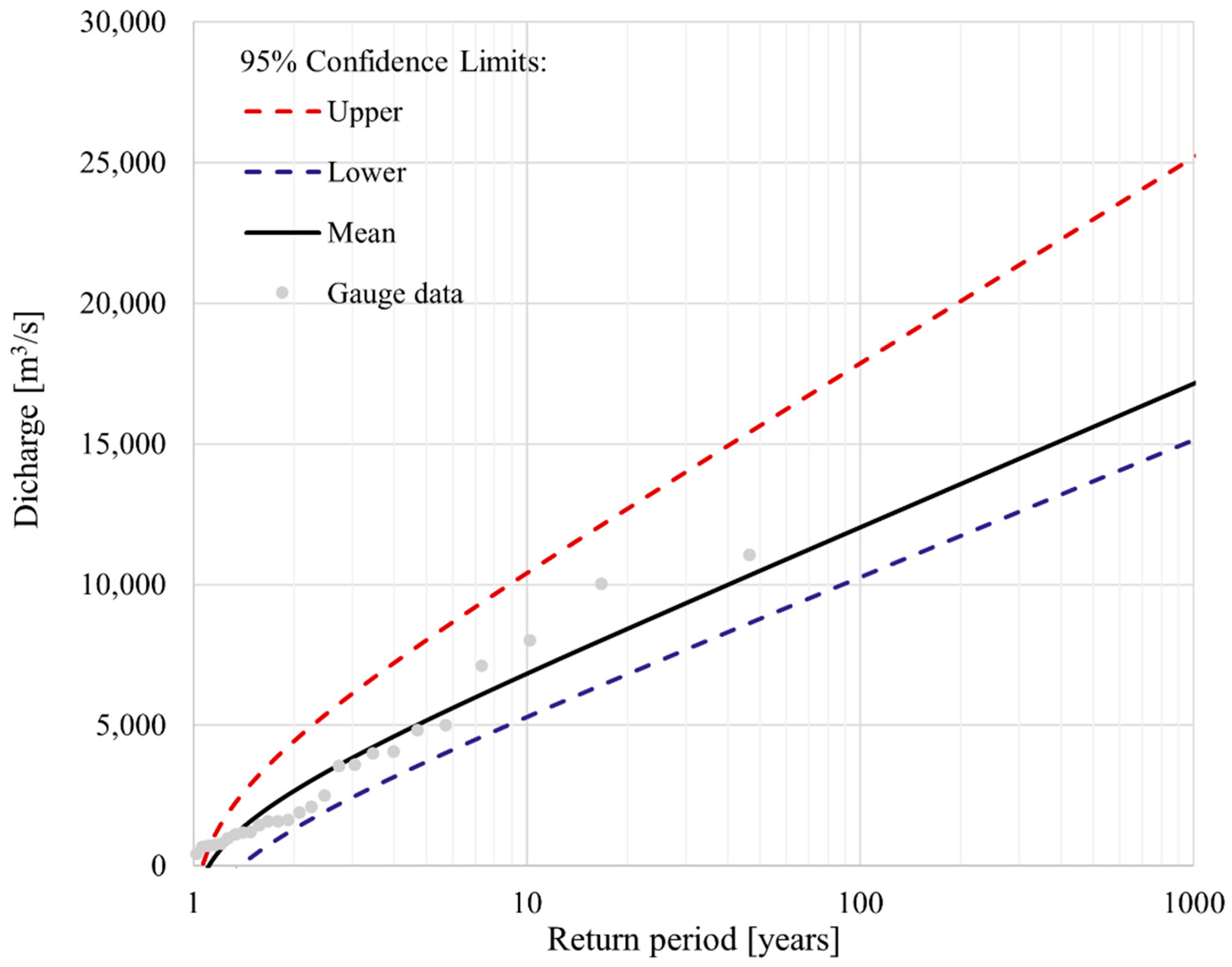
3.1.1. Use of Bridge Failure Data for a Temporal Probability Assessment
3.1.2. Flood Hazard Assessment on a Local Level
3.1.3. Natural Hazards at Regional Level
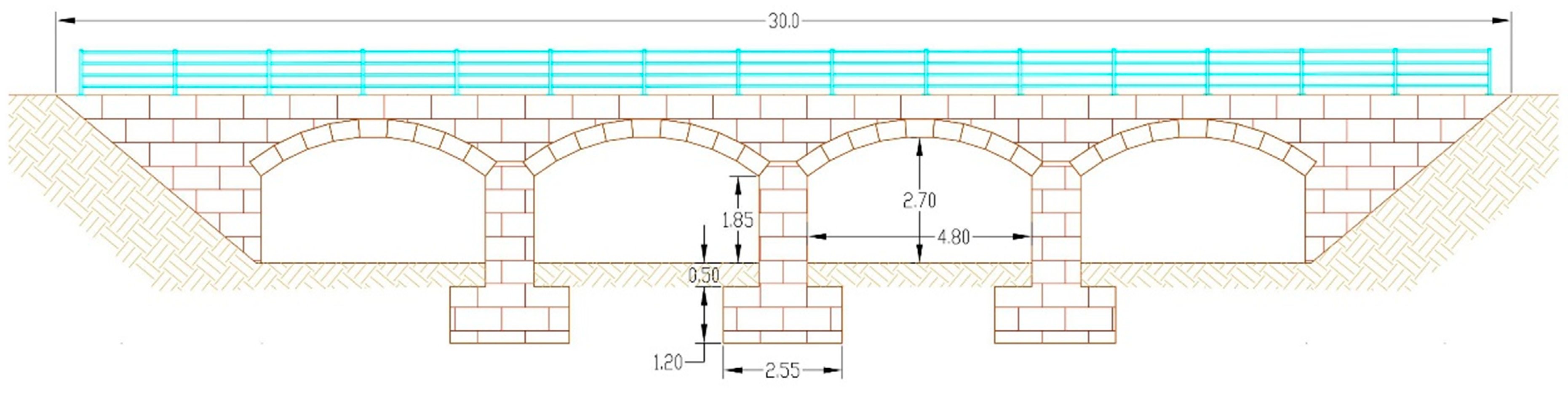
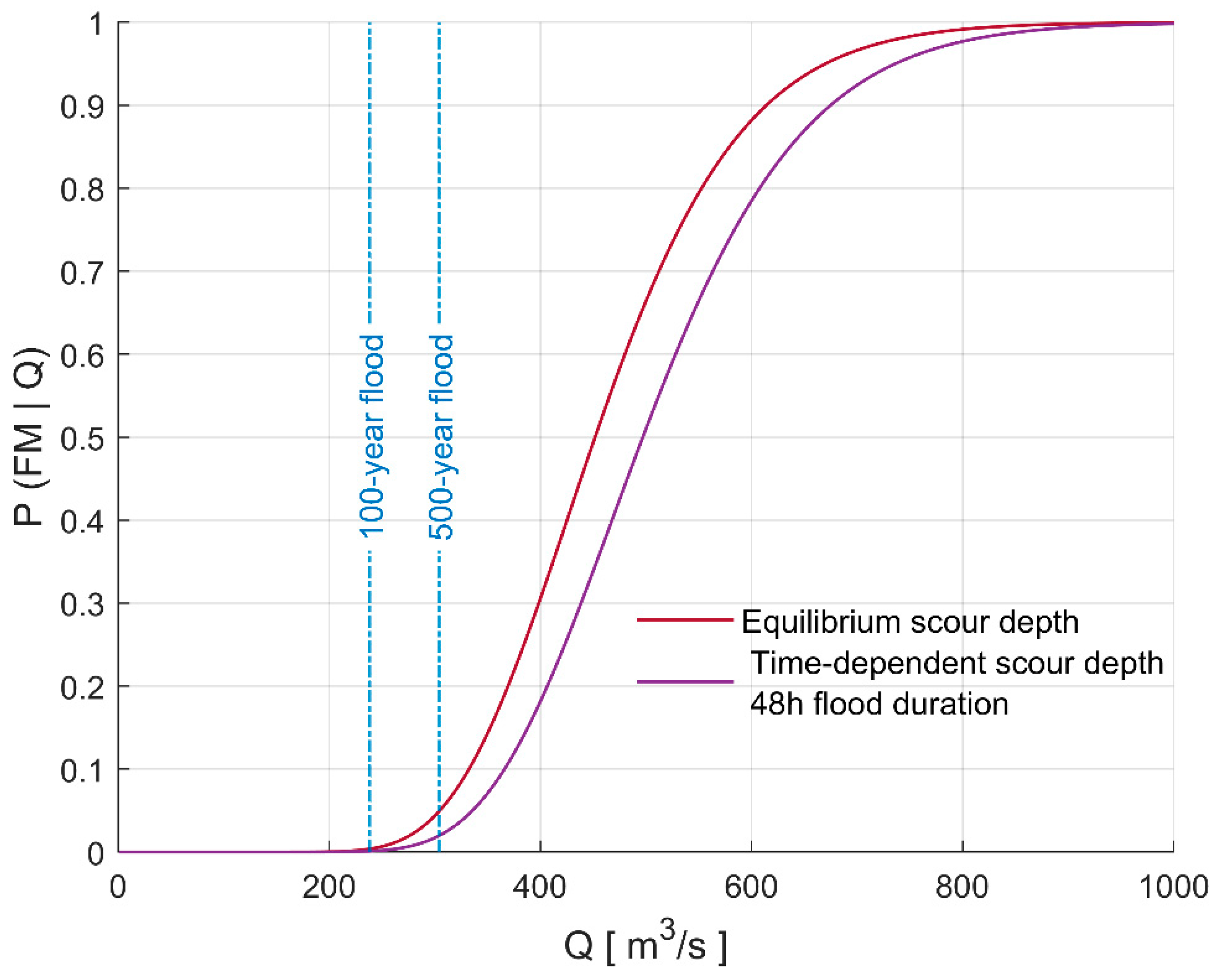
3.2. Vulnerability Assessment Example of an Asset-Specific Assessment of a Fragility Curve—A Case of a Bridge Scour in Portugal
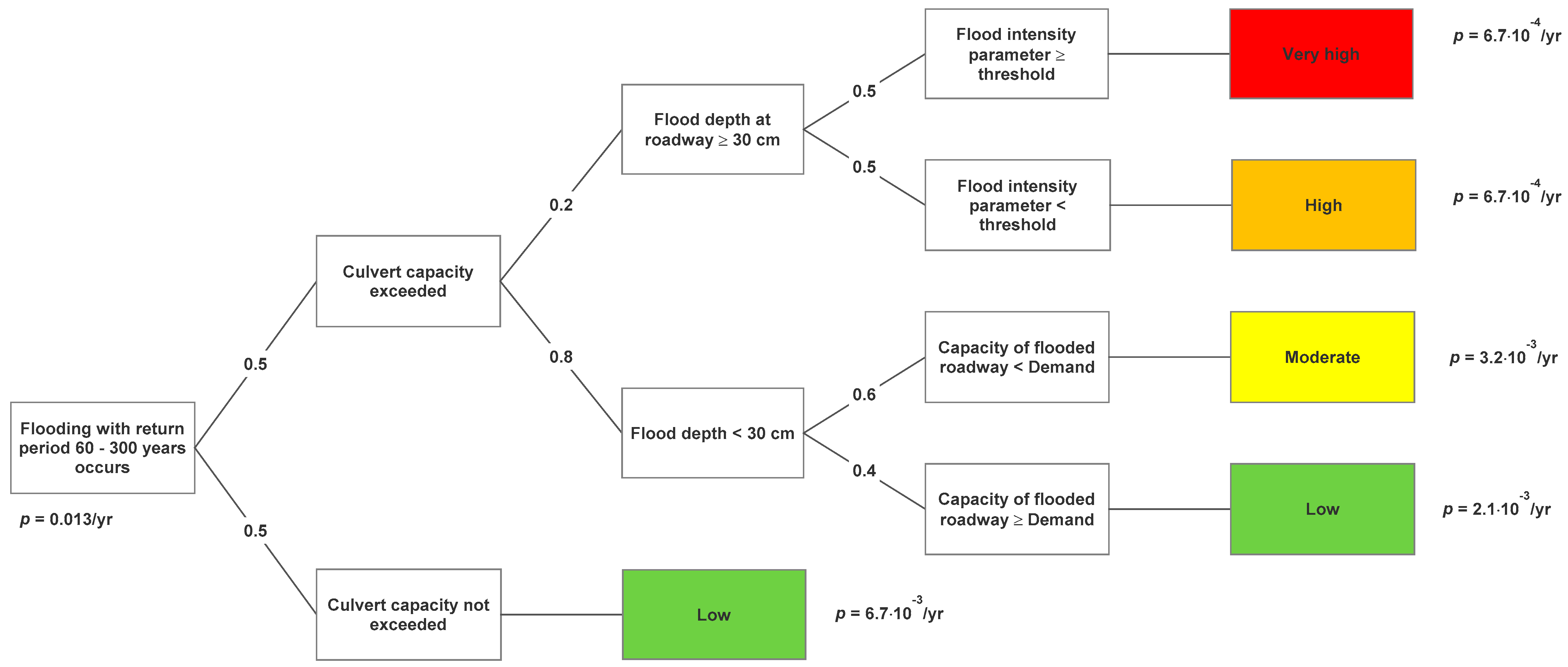
3.3. Risk Assessment Example: Asset Failure and Related Service Disruption
- What is the return period of the flooding event that may pose a threat?
- Is the culvert capacity exceeded?
- Will flooding of the road cause full service disruption?
- Will flooding cause material damage?
- Is the capacity reduced below demand?
- How severe are the consequences?
- Very high consequences: A flood depth higher than 30 cm, velocity of the flooding water high enough to cause material damage to the roadway.
- High consequences: A flood depth higher than 30 cm, velocity of the flooding water not high enough to cause material damage to the roadway.
- Moderate consequences: A flood depth less than 30 cm. The capacity of the roadway is reduced to less than the demand.
- Low consequences: A flood depth less than 30 cm. The capacity of the roadway is larger than the demand (including the case where the culvert capacity is not exceeded).
4. Discussion
5. Conclusions
Author Contributions
Funding
Institutional Review Board Statement
Informed Consent Statement
Data Availability Statement
Conflicts of Interest
Disclaimer
References
- Mattsson, L.G.; Jenelius, E. Vulnerability and resilience of transport systems—A discussion of recent research. Transp. Res. Part A 2015, 81, 16–34. [Google Scholar] [CrossRef]
- Hackl, J.; Lam, J.C.; Heitzler, M.; Adey, B.; Hurni, L. Estimating network related risks, A methodology and an application in the transport sector. Nat. Hazards Earth Syst. Sci. 2018, 18, 2273–2293. [Google Scholar] [CrossRef] [Green Version]
- Dobney, K.; Baker, C.J.; Quinn, A.D.; Chapman, L. Quantifying the effects of high summer temperatures due to climate change on buckling and rail related delays in south-east United Kingdom. Meteorol. Appl. 2009, 16, 245–251. [Google Scholar] [CrossRef]
- Kontou, E.; Murray-Tuite, P.; Wernstedt, K. Duration of commute travel changes in the aftermath of Hurricane Sandy using accelerated failure time modeling. Transport. Res. A Policy Pract. 2017, 100, 170–181. [Google Scholar] [CrossRef] [Green Version]
- Pregnolato, M.; Ford, A.; Wilkinson, S.M.; Dawson, R.J. The impact of flooding on road transport, A depth-disruption function. Transp. Res. Part D 2017, 55, 67–81. [Google Scholar] [CrossRef]
- Eidsvig, U.; Kristensen, K.; Vangelsten, B.V. Assessing the risk posed by natural hazards to infrastructures. Nat. Hazards Earth Syst. Sci. 2017, 17, 481–504. [Google Scholar] [CrossRef] [Green Version]
- Lam, J.C.; Adey, B.T.; Heitzler, M.; Hackl, J.; Gehl, P.; van Erp, N.; D’Ayala, D.; van Gelder, P.; Hurni, L. Stress tests for a road network using fragility functions and functional capacity loss functions. Reliab. Eng. Syst. Saf. 2018, 173, 78–93. [Google Scholar] [CrossRef]
- Winter, M.G.; Smith, J.T.; Fotopoulou, S.; Pitilakis, K.; Mavrouli, O.; Corominas, J.; Argyroudis, S. An expert judgement approach to determining the physical vulnerability of roads to debris flow. Bull. Eng. Geol. Environ. 2014, 73, 291–305. [Google Scholar] [CrossRef]
- Oberndorfer, S.; Sander, P.; Fuchs, S. Multi-hazard risk assessment for roads, probabilistic versus deterministic approaches. Nat. Hazards Earth Syst. Sci. 2020, 20, 3135–3160. [Google Scholar] [CrossRef]
- Mitsakis, E.; Stamos, I.; Papanikolaou, A.; Aifadopoulou, G.; Kontoes, H. Assessment of extreme weather events on transport networks, case study of the 2007 wildfires in Peloponnesus. Nat. Hazards 2014, 72, 87–107. [Google Scholar] [CrossRef]
- EEA. Climate Change, Impacts and Vulnerability in Europe 2016, An Indicator-Based Report; European Environment Agency (EEA), 2017. Available online: www.eea.europa.eu (accessed on 19 September 2018).
- WMO; UNISDR. Disaster Risk and Resilience, UN System Task Team on the Post-2015 UN Development Agenda. 2012. Available online: https://www.un.org/en/development/desa/policy/untaskteam_undf/thinkpieces/3_disaster_risk_resilience.pdf (accessed on 6 June 2021).
- Chen, L.; Wu, H.; Liu, T. Vehicle collision with bridge piers, A state-of the-art review. Adv. Struct. Eng. 2021, 24, 385–400. [Google Scholar] [CrossRef]
- Sha, Y.; Hao, H. Nonlinear finite element analysis of barge collision with a single bridge pier. Eng. Struct. 2012, 41, 63–76. [Google Scholar] [CrossRef]
- Wang, W.; Liu, R.; Wu, B. Analysis of a bridge collapsed by an accidental blast loads. Eng. Fail. Anal. 2014, 36, 353–361. [Google Scholar] [CrossRef]
- Giuliani, L.; Crosti, C.; Gentili, F. Vulnerability of Bridges to Fire. Bridge Maintenance, Safety, Management, Resilience and Sustainability. In Proceedings of the Sixth International Conference on Bridge Maintenance, Safety and Management, Stresa, Lake Maggiore, Italy, 8–12 July 2012. [Google Scholar]
- VTT. Extreme Weather Impacts on Transport Systems. VTT Working Papers 168, EWENT Project Deliverable D1. 2011. Available online: http://www.vtt.fi/publications/index.jsp (accessed on 20 September 2018).
- Erath, A.L. Vulnerability Assessment of Road Transport Infrastructure. Ph.D. Thesis, ETH, Zürich, Switzerland, 2011. Available online: www.research-collection.ethz.ch/handle/20.500.11850/153072 (accessed on 30 October 2019).
- Meyer, V.; Becker, N.; Markantonis, V.; Schwarze, R.; van den Bergh, J.C.J.M.; Bouwer, L.M.; Bubeck, P.; Ciavola, P.; Genovese, E.; Green, C.; et al. Review article, Assessing the costs of natural hazards–state of the art and knowledge gaps. Nat. Hazards Earth Syst. Sci. 2013, 13, 1351–1373. [Google Scholar] [CrossRef]
- Liu, L.; Yang, D.Y.; Frangopol, D.M. Network-level risk-based framework for optimal bridge adaptation management considering scour and climate change. J. Infrastruct. Syst. 2020, 26, 516. [Google Scholar] [CrossRef]
- Santarsiero, G.; Masi, A.; Digrisolo, V.; Picciano, A. The Italian Guidelines on Risk Classification and Management of Bridges, Applications and Remarks on Large Scale Risk Assessments. Infrastructures 2021, 6, 111. [Google Scholar] [CrossRef]
- Pregnolato, M. Bridge safety is not for granted—A novel approach to bridge management. Eng. Struct. 2019, 196, 35. [Google Scholar] [CrossRef]
- Technical Committee ISO/TC 262, Risk Management. In ISO 31000:2018 Risk Management—Guidelines; ISO (The International Organization for Standardization): Geneva, Switzerland, 2018; Available online: https://www.iso.org/standard/65694.html (accessed on 7 July 2021).
- Snelder, M.; Calvert, S. Quantifying the impact of adverse weather conditions on road network performance. Eur. J. Transp. Infrastruct. Res. 2016, 1, 128–149. [Google Scholar]
- Düzgün, H.S.B.; Lacasse, S. Vulnerability and Acceptable Risk in Integrated Risk Assessment Framework. In Landslide Risk Management; A.A. Balkema Publishers: Vancouver, BC, Canada, 2005. [Google Scholar]
- Falermo, S.; Blied, L.; Danielsson, P. Guideline-Part C, GIS-Aided Vulnerability Assessment for Roads–Existing Methods and New Suggestions; Roadapt Report; SGI: Linköping, Sweden, 2015. [Google Scholar]
- Koks, E.E.; Bockarjova, M.; de Moel, H.; Aerts, J.C.J.H. Integrated Direct and Indirect Flood Risk Modeling, Development and Sensitivity Analysis. Risk Anal. 2014, 35, 882–900. [Google Scholar] [CrossRef] [PubMed] [Green Version]
- Kilanitis, I.; Sextos, A. Integrated seismic risk and resilience assessment of roadway networks in earthquake prone areas. Bull. Earthq. Eng. 2019, 17, 181–210. [Google Scholar] [CrossRef] [Green Version]
- Messore, M.M.; Capacci, L.; Biondini, F. Life-cycle cost-based risk assessment of aging bridge networks. Struct. Infrastruct. Eng. 2020, 17, 515–533. [Google Scholar] [CrossRef]
- Pregnolato, M.; Winter, A.O.; Mascarenas, D.; Sen, A.D.; Bates, P.; Motley, M.R. Assessing flooding impact to riverine bridges, an integrated analysis. Nat. Hazards Earth Syst. Sci. Discuss. 2020. preprint. [Google Scholar] [CrossRef]
- Yang, D.Y.; Frangopol, D.M. Physics-based assessment of climate change impact on long-term regional bridge scour risk using hydrologic modeling, Application to Lehigh River watershed. J. Bridge. Eng. 2019, 24, 13. [Google Scholar] [CrossRef]
- Akiyama, M.; Frangopol, D.M.; Ishibashi, H. Toward lifecycle reliability-, risk- and resilience-based design and assessment of bridges and bridge networks under independent and interacting hazards, emphasis on earthquake, tsunami and corrosion. Struct. Infrastruct. Eng. 2019, 16, 26–50. [Google Scholar] [CrossRef]
- Ishibashi, H.; Akiyama, M.; Frangopol, D.M.; Koshimura, S.; Kojima, T.; Nanami, K. Framework for estimating the risk and resilience of road networks with bridges and embankments under both seismic and tsunami hazards. Struct. Infrastruct. Eng. 2020, 17, 494–514. [Google Scholar] [CrossRef]
- Argyroudis, S.A.; Mitoulis, S.A.; Winter, M.G.; Kaynia, A.M. Fragility of transport assets exposed to multiple hazards, State-of-the-art review toward infrastructural resilience. Reliab. Eng. Syst. Saf. 2019, 191, 22. [Google Scholar] [CrossRef]
- Kim, H.; Sim, S.H.; Lee, J.; Lee, Y.J.; Kim, J.M. Flood fragility analysis for bridges with multiple failure modes. Adv. Mech. Eng. 2017, 9, 1687814017696415. [Google Scholar] [CrossRef] [Green Version]
- Lamb, R.; Aspinall, W.; Odbert, H.; Wagener, T. Vulnerability of bridges to scour, insights from an international expert elicitation workshop. Nat. Hazards Earth Syst. Sci. 2017, 17, 1393–1409. [Google Scholar] [CrossRef] [Green Version]
- Tanasic, N. Vulnerability of Reinforced Concrete Bridges Exposed to Local Scour in Bridge Management. Ph.D. Thesis, University of Belgrade, Belgrade, Serbia, 2015. [Google Scholar]
- Tsubaki, R.; Bricker, J.D.; Ichii, K.; Kawahara, Y. Development of fragility curves for railway embankment and ballast scour due to overtopping flood flow. Nat. Hazards Earth. Syst. Sci. 2016, 16, 2455–2472. [Google Scholar] [CrossRef] [Green Version]
- McKenna, G.; Argyroudis, S.A.; Winter, M.G.; Mitoulis, S.A. Multiple hazard fragility analysis for granular highway embankments, Moisture ingress and scour. Transp. Geotech. 2021, 26, 1143. [Google Scholar] [CrossRef]
- Gehl, P.; D’Ayala, D. System loss assessment of bridge networks accounting for multi-hazard interactions. Struct. Infrastruct. Eng. 2018, 14, 1355–1371. [Google Scholar] [CrossRef] [Green Version]
- Starossek, U.; Haberland, M. Disproportionate collapse: Terminology and procedures. J. Perform. Constr. Facil. 2010, 24, 519–528. [Google Scholar] [CrossRef] [Green Version]
- Van Westen, C.J.; Castellanos Abella, E.A.; Sekhar, L.K. Spatial data for landslide susceptibility, hazards and vulnerability assessment, an overview. Eng. Geol. 2008, 102, 112–131. [Google Scholar] [CrossRef]
- Nadim, F. Risk Assessment and Management for Geohazards, Keynote Lecture, 2nd ed.; Symposium on Geotechnical Safety & Risk; CRC Press/Balkema: Gifu, Japan, 2009; pp. 13–26. [Google Scholar]
- Ministerio Para la Transición Ecológica. Available online: https://www.miteco.gob.es/es/agua/temas/gestion-de-los-riesgos-de-inundacion/mapa-peligrosidad-riesgo-inundacion/ (accessed on 5 April 2019).
- AASHTO. LRFD Bridge. Design Specifications; American Association of State Highway and Transportation Officials (AASHTO): Washington, DC, USA, 2012. [Google Scholar]
- Hajdin, R.; Kušar, M.; Mašović, S.; Linneberg, P.; Amado, J.; Tanasić, N. WG3 Technical Report, Establishment of a Quality Control Plan. COST TU 1406. 2018. Available online: https://www.tu1406.eu/wp-content/uploads/2018/09/tu1406_wg3_digital_vf.pdf (accessed on 31 October 2018).
- Li, Z.; Nadim, F.; Huang, H.; Uzielli, M.; Lacasse, S. Quantitative vulnerability estimation for scenario based landslide hazards. Landslides 2010, 7, 125–134. [Google Scholar] [CrossRef]
- Cardona, O.D.; van Aalst, M.K.; Birkmann, J.; Fordham, M.; McGregor, G.; Perez, R.; Pulwarty, R.S.; Schipper, E.L.F.; Sinh, B.T. Determinants of risk, exposure and vulnerability. In Managing the Risks of Extreme Events and Disasters to Advance Climate Change Adaptation. In A Special Report of Working Groups I and II of the Intergovernmental Panel on Climate Change (IPCC); Cambridge University Press: London, UK, 2012; pp. 65–108. [Google Scholar]
- Schultz, M.T.; Gouldby, B.P.; Simm, J.D.; Wibowo, J.L. Beyond the Factor of Safety, Developing Fragility Curves to Characterize System Reliability; Army Corps of Engineers: Washington, DC, USA, 2010. [Google Scholar]
- Schneiderbauer, S.; Calliari, E.; Eidsvig, U.; Hagenlocher, M. The most recent view of vulnerability. In Science for Disaster Risk Management 2017, Knowing Better and Loosing Less; Publications Office of the European Union: Luxembourg, 2017; pp. 70–84. [Google Scholar]
- Chapman, L.; Thornes, J.E.; Huang, Y.; Cai, X.; Sanderson, V.L.; White, S.P. Modelling of rail surface temperatures, a preliminary study. Theor. Appl. Climatol. 2008, 92, 121–131. [Google Scholar] [CrossRef]
- Dobney, K.; Baker, C.J.; Chapman, L.; Quinn, A.D. The future cost to the United Kingdom’s railway network of heat-related delays and buckles caused by the predicted increase in high summer temperatures owing to climate change. Proc. Inst. Mech. Eng. Part F 2009, 224, 25–34. [Google Scholar] [CrossRef]
- NetworkRail. Route Weather Resilience and Climate Change Adaptation Plans, London North. West.; NetworkRail: London, UK, 2014. [Google Scholar]
- Vajda, A.; Tuomenvirta, H.; Juga, I.; Nurmi, P.; Jokinen, P.; Rauhala, J. Severe weather affecting European transport systems, the identification, classification and frequencies of events. Nat. Hazards 2014, 72, 169–188. [Google Scholar] [CrossRef]
- Argyroudis, S.A.; Mitoulis, S.A. Vulnerability of bridges to individual and multiple hazards-floods and earthquakes. Reliab. Eng. Syst. Saf. 2010, 210, 107564. [Google Scholar] [CrossRef]
- ASTRA. Naturgefahren auf den Nationalstrassen, Risikokonzept. Dokumentation ASTRA 89001, Guidelines; Swiss Federal Roads Office (Bundesamt für Strassen): Bern, Switzerland, 2012.
- UNSW. Vehicle Stability Testing for Flood Flows; WRL Technical Report 2017/07; Water Research Laboratory, University of New South Wales: New South Wales, Australia, 2017. [Google Scholar]
- El-Tawil, S.; Severino, E. Vehicle Collision with Bridge Piers. J. Bridge. Eng. 2005, 10, 637–640. [Google Scholar] [CrossRef] [Green Version]
- Pasha, J.; Dulebenets, M.A.; Abioye, O.F.; Kavoosi, M.; Moses, R.; Sobanjo, J.; Ozguven, E.E. A comprehensive assessment of the existing accident and hazard prediction models for the highway-rail grade crossings in the state of Florida. Sustainability 2020, 12, 4291. [Google Scholar] [CrossRef]
- Alos-Moya, J.; Paya-Zaforteza, I.; Garlock, M.E.M.; Loma-Ossorio, E.; Schiffner, D.; Hospitaler, A. Analysis of a bridge failure due to fire using computational fluid dynamics and finite element models. Eng. Struct. 2014, 68, 96–110. [Google Scholar] [CrossRef]
- Lange, D.; Sjöström, J.; Honfi, D. Losses and Consequences of Large Scale Incidents with Cascading Effects. In EU FP 7 Project CascEff Modelling of Dependencies and Cascading Effects for Emergency; CascEff Project: Vienna, Austria, 2015. [Google Scholar]
- Martins, L.; Silva, V. Development of a fragility and vulnerability model for global seismic risk analyses. Bull. Earthq. Eng. 2020, 7, 8851. [Google Scholar] [CrossRef]
- Papathoma-Köhle, M.; Kappes, M.; Keiler, M.; Glade, T. Physical vulnerability assessment for alpine hazards, state of the art and future needs. Nat. Hazards 2011, 58, 645–680. [Google Scholar] [CrossRef]
- Erath, A.; Birdsall, J.; Axhausen, K.W.; Hajdin, R. Vulnerability assessment of the Swiss road network. Transp. Res. Rec. 2009, 2137, 118–128. [Google Scholar] [CrossRef]
- Pregnolato, M.; Ford, A.; Robson, C.; Glenis, V.; Barr, S.; Dawson, R. Assessing urban strategies for reducing the impacts of extreme weather on infrastructure networks. R. Soc. Open Sci. 2016, 3, 160023. [Google Scholar] [CrossRef] [PubMed] [Green Version]
- Tanasic, N.; Ilic, V.; Hajdin, R. Vulnerability assessment of bridges exposed to scour. Transp. Res. Rec. J. Transp. Res. Board 2013, 2360, 36–44. [Google Scholar] [CrossRef]
- Santamaria, M.; Arango, E.; Jafari, F.; Sousa, H. SAFEWAY consortium. In Dynamic Risk-Based Predictive Models; SAFEWAY Deliverable 5.1; SAFEWAY Project: Vigo, Spain, 2021. [Google Scholar]
- Hoogendoorn, S.; Knoop, V. Traffic flow theory and modelling. In The Transport System and Transport Policy; Edward Elgar Publishing: Cheltenham, UK, 2012; pp. 125–159. [Google Scholar]
- Nogal, M.; Honfi, D. Assessment of road traffic resilience assuming stochastic user behaviour. Reliab. Eng. Syst. Saf. 2019, 185, 72–83. [Google Scholar] [CrossRef]
- Wardrop, J.G. Some theoretical aspects or road traffic research. Road Eng. Div. Meet. Road Pap. 1952, 36, 325–378. [Google Scholar] [CrossRef]
- Syrkov, A.; Høj, N.P. Bridge failures analysis as a risk mitigating tool. In IABSE Symposium, Towards a Resilient Built Environment -Risk and Asset; IABSE: Guimarães, Portugal, 2019; pp. 304–310. [Google Scholar]
- Galvão, N.; Matos, J.; Oliveira, D.V. Human Errors induced risk in reinforced concrete bridge engineering. J. Perform. Constr. Facil. 2021, 35, 4. [Google Scholar]
- Proske, D. Bridge. Collapse Frequencies versus Failure Probabilities; Springer International Publishing: Cham, Switzerland, 2018. [Google Scholar]
- CEN. EN 1990, Eurocode 0, Basis of Structural Design; European Committee for Standardization (CEN): Brussels, Belgium, 2002. [Google Scholar]
- Joint Committee on Structural Safety. Probabilistic Model. Code—Part. 1, Basis of Design. 2001. Available online: https://www.jcss-lc.org/jcss-probabilistic-model-code/ (accessed on 3 September 2020).
- Centre for Ecology and Hydrology. Flood Estimation Handbook; Centre for Ecology and Hydrology (Formerly the Institute of Hydrology): Wallingford, UK, 1999. [Google Scholar]
- England, J.F.; Cohn, T.A.; Faber, B.A.; Stedinger, J.R.; Thomas, W.O.; Veilleux, A.G.; Kiang, J.E.; Mason, R.R. Guidelines for determining flood flow frequency—Bulletin 17C (ver. 1.1, May 2019). USA Geol. Surv. Tech. Methods 2019, 5, 148. [Google Scholar] [CrossRef] [Green Version]
- Tejo, A.R.H. Plano de Gestão da Região Hidrográfica do Tejo Relatório Técnico; Agência Portuguesa do Ambiente (APA): Amadora, Portugal, 2012. [Google Scholar]
- Parkes, B.; Demeritt, D. Defining the hundred year flood, A Bayesian approach for using historic data to reduce uncertainty in flood frequency estimates. J. Hydrol. 2016, 540, 1189–1208. [Google Scholar] [CrossRef] [Green Version]
- Eidsvig, U.; Piciullo, L.; Ekseth, K.; Ekeheien, C. SAFEWAY consortium. European critical hazards (natural), GIS Map and identification of hot spots of sudden extreme natural hazard events, including database with impact and return periods. In SAFEWAY Deliverable D2.1; SAFEWAY Project: Vigo, Spain, 2019. [Google Scholar]
- Zampieri, P.; Zanini, M.A.; Faleschini, F.; Hofer, L.; Pellegrino, C. Failure analysis of masonry arch bridges subject to local pier scour. Eng. Fail. Anal. 2017, 79, 371–384. [Google Scholar] [CrossRef]
- Tanasic, N.; Hajdin, R. Management of RC bridges with shallow foundation exposed to local scour. J. Struct. Infrastruct. Eng. 2017, 14, 468–476. [Google Scholar] [CrossRef]
- Scozzese, F.; Ragni, L.; Tubaldi, E.; Gara, F. Modal properties variation and collapse assessment of masonry arch bridges under scour action. Eng. Struct. 2019, 199, 109665. [Google Scholar] [CrossRef]
- Lagasse, P.F.; Ghosn, M.; Johnson, P.A.; Zevenbergen, L.W.; Clopper, P.E. Risk-Based Approach for Bridge Scour Prediction; National Cooperative Highway Research Program Transportation Research Board National Research Council: Washington, DC, USA, 2013. [Google Scholar]
- Uzielli, M.; Lacasse, S.; Nadim, F.; Phoon, K.K. Soil variability analysis for geotechnical practice. Charact. Eng. Prop. Nat. Soils 2007, 22, 1653–1754. [Google Scholar] [CrossRef]
- Conde, B.; Matos, J.; Oliveira, D.; Riveiro, B. Probabilistic-based structural assessment of a historic stone arch bridge. Struct. Infrastruct. Eng. 2020, 17, 379–391. [Google Scholar] [CrossRef]
- Sheppard, D.M.; Renna, R. Bridge. Scour Manual; State of Florida Department of Transportation: Tallahassee, FL, USA, 2010.
- Smith, C.; Gilbert, M. Application of discontinuity layout optimization to plane plasticity problems. Proc. R. Soc. A 2007, 463, 2461–2484. [Google Scholar] [CrossRef] [Green Version]
- LimitState. Geotechnical Analysis Software. 2019. Available online: https://www.limitstate.com/geo (accessed on 30 January 2021).
- Ioannou, I.; Rossetto, T.; Grant, D.N. Use of Regression Analysis for the Construction of Empirical Fragility Curves. In Proceedings of the Fifteenth World Conference on Earthquake Engineering, Lisbon, Portugal, 24–28 September 2012. [Google Scholar]
- ISO. IEC 31010:2019 Risk Management—Risk Assessment Techniques. Technical Committee, ISO/TC 262 Risk Management. 2019. Available online: https://www.iso.org/standard/72140.html (accessed on 7 July 2021).
- Adey, B.; Birdsall, J.; Hajdin, R. Methodology to Estimate Risk Related to Road Links, due to Latent Processes. In Proceedings of the 5th International Conference on Bridge Maintenance, Safety and Management IABMAS, Philadelphia, PA, USA, 11–14 July 2010. [Google Scholar]
- Hajdin, R.; Lindenmann, H. Algorithm for the Planning of Optimum Highway Work Zones. J. Infrastruct. Syst. 2007, 13, 202–214. [Google Scholar] [CrossRef]
- Pyatkova, K.; Chen, A.S.; Butler, D.; Vojinović, Z.; Djordjević, S. Assessing the knock-on effects of flooding on road transportation. J. Environ. Manag. 2019, 244, 48–60. [Google Scholar] [CrossRef] [PubMed]


| Failure Modes/Modes of Malfunctioning | ||||
|---|---|---|---|---|
| Extreme Events | Structural Damage of Assets | Material or Obstacles on the Transportation Line | Failure in Supporting Systems | Other Dangerous Driving Conditions (Including Precautionary Closure) |
| Heat waves | Road: damage to pavement Railway: rail buckling | n.a. | Overheating of equipment | n.a. |
| Forest fires | Damages and deformations due to heat | n.a. | Overheating of equipment | Reduced visibility |
| Heavy precipitation | Damage to slope or embankment due to mass transport by surface water | n.a. | n.a. | Reduced visibility and reduced road surface friction |
| Flooding (urban, river, flash floods, storm surge) | Erosion of embankment, damage to bridge supports (e.g., scour) | Water on transportation line and in underground transport system | n.a. | Reduced road surface friction |
| Gravitational mass movements (Landslides, rock-falls, etc.) | Damage to road/rail sections, damages to bridges, embankments, etc. | Blocking of transportation line by soil/rock masses | Failure of signal systems | Load posting or line closure due to increase in occurrence probability of mass movements |
| Fog | n.a. | n.a. | n.a. | Reduced visibility |
| Storms (thunderstorms, hail, blizzards, i.e., strong wind gusts, intense snowfall) | n.a. | Unavailability of transportation line due to snow or obstacles on the transportation lines (e.g., falling trees) | Damage to support systems (e.g., owing to falling trees) | Reduced visibility and surface friction; strong wind gusts, especially on bridges, may lead to overturning of vehicles |
| Cold spells | “Thermal fatigue”; frost heave; asphalt of pavement Cracking, contractions of components | n.a. | Malfunction of signaling due to low temperatures | Technical failure of vehiclesReduced surface friction |
| Surface motions from, e.g., subsidence, sinkholes, uplift and swelling | Damage to road/rail sections, damages to bridges, tunnels, etc. | n.a. | Failure of signal systems | Load/speed posting or line closure (to prevent potential hazard trigger or reduce potential consequences to users) |
| Ship and vehicle collisions against bridges (or other assets) | Buckling of piers, deck overturning, failure of supports, etc. | Interruption of the underpass and/or overpass | n.a. | Vibrations and/or large deflections |
| Highway-railway grade-crossing accidents/incidents | Damage to the rail track or pavement | Obstacles on the transportation lines (e.g., damaged vehicles, injured people) | Damage to support systems (e.g., rail safety-guards, traffic lights) | Vibrations and/or large deflections |
| Explosion (i.e., gas explosion and vehicles on fire) | Damage to assets (resistance reduction due to high temperatures, dynamic loads) | Interruption caused by debris from the explosion or fire | Damage to support systems (e.g., rail safety-guards, traffic lights) | Reduced visibility caused by smoke |
| Overview of Available Damage, Loss and Fragility Models | |||
|---|---|---|---|
| Extreme Event | Structural Damage of Assets | Material or Obstacles on the Transportation Line | Dangerous Driving Conditions (Including Precautionary Closure) |
| Heat waves | Temperature threshold models for rail buckling: [3,51,52,53] | n.a. | Probability of adverse events for different threshold values of temperature: [54] |
| Flooding (urban, river, flash floods, storm surge) | Bridge scour leading to bridge failure: [35,36,37,55] Ballast scour and failure: [38] Roadway embankment scour: [39] Material damage to roads: [56] | Vehicle speed as function of floodwater depth: [5] Functional capacity loss functions as a function of inundation depth: [2,7] | Thresholds for vehicle stability in floods: [57] |
| Landslides | Material damage to roads: [9,56] | Malfunctioning due to debris on roads as a function of landslide volume: [8] | n.a. |
| Storms | n.a. | Probability of adverse events for different threshold values of wind speed: [54] | Threshold models for wind speed on bridges: [53] |
| Ship and vehicle collisions against bridges | Vehicle collision with bridge piers: [58] Vehicle collision with bridge piers: A state-of-the-art review: [13] Nonlinear finite element analysis of barge collision with a single bridge pier: [14] | n.a. | n.a. |
| Highway-rail grade-crossing accidents/incidents | A comprehensive assessment of the existing accident and hazard prediction models for the highway-rail grade crossings in the state of Florida: [59]. | n.a. | n.a. |
| Explosion (i.e., gas explosion), bombing and vehicles on fire | Vulnerability of bridges to fire: [16] Analysis of a bridge failure due to fire using computational fluid dynamics and finite element models: [60] Analysis of a bridge collapsed by accidental blast loads: [15] | n.a. | n.a. |
| Extreme Event/Hazard | Asset | ||
|---|---|---|---|
| Type | Modelling Variable | Type | Failure Mode |
| Flooding | Water discharge | Bridge | Bridge scour leading to bridge failure |
| Flooding | Water discharge | Culvert | Failure of culvert leading to water overtopping and material damage to road/rail |
| Flooding | Water discharge | Embankment | Failure of embankment caused by erosion |
| Flooding | Water discharge | Roadway or rail track | Wash-out of roadway/rail track |
| Rainfall/urban flooding | Water depth | Roadway | Speed and capacity reductions/service disruption due to water on road |
| Flooding | Volume of debris | Roadway or rail track | Speed and capacity reductions/service disruption due to debris on road/track after flooding |
| Landslide | Volume of landslides | Roadway or rail track | Speed and capacity reductions/service disruption due to landslide masses on road/track |
| Heatwave | Temperature | Rail track | Speed reductions of trains to avoid buckling of tracks |
| Wind | Wind speed perpendicular to the bridge | Bridge | Closed bridges due to strong wind gusts |
| Ship and vehicle collisions against bridges | Impact force | Bridge | Failure, collapse, damaged element |
| Highway-rail grade-crossing accidents/incidents | Down time and restricted lanes | Roadway or rail track | Closed or traffic reduction/failure, collapse, damaged element |
| Explosion (i.e., gas explosion and vehicles on fire) | Pressure-impulse | All types of assets | Closed or traffic reduction/failure, collapse, damaged element |
| Period | Recorded Failures | Percentage | Failure Frequency * | |||
|---|---|---|---|---|---|---|
| NHs | HMHs | D & CEs | OEs | |||
| 1966–1970 | 10 | 1.5% | ||||
| 1971–1975 | 18 | 2.7% | ||||
| 1976–1980 | 38 | 5.8% | ||||
| 1981–1985 | 13 | 2.0% | ||||
| 1986–1990 | 20 | 3.0% | ||||
| 1991–1995 | 16 | 2.4% | ||||
| 1996–2000 | 21 | 3.2% | ||||
| 2001–2005 | 65 | 9.9% | ||||
| 2006–2010 | 108 | 16.4% | ||||
| 2011–2015 | 157 | 23.9% | ||||
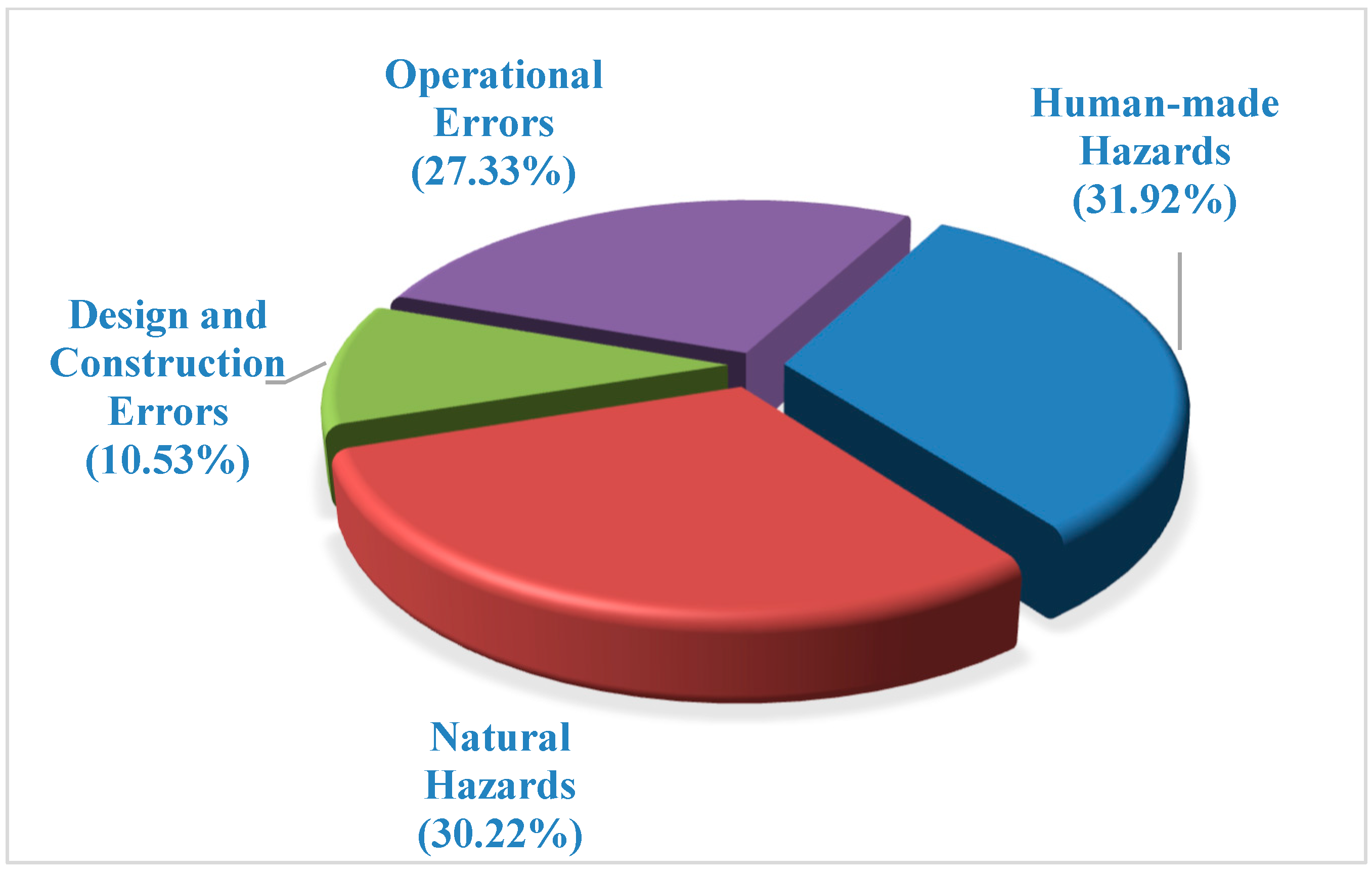
| 2016–2020 | 191 | 29.1% | 1.92 × 10⁻⁵ | 1.86 × 10⁻⁵ | 2.79 × 10⁻⁶ | 1.40 × 10⁻⁵ |
| Total | 657 | 100% ** | ||||
| Total Bridge Stock: 3.225.047 [73] | ||||||
| Parameters | Mean 1 [Units] | COV | Distribution | Reference 2 | |
|---|---|---|---|---|---|
| Local scour action | Peak discharge | 74.6 [m3/s] | 0.70 | Gumbel | [78] |
| Peak flood duration | 48 [h] | - | - | Assumed | |
| Channel width | 30 [m] | 0.05 | Normal | Assumed | |
| Channel bed slope | 0.002 [m/m] | 0.10 | Normal | Assumed | |
| Manning roughness coefficient | 0.035 [s/m1/3] | 0.015 | Lognormal | [84] | |
| Riverbed mean size diameter | 20 [mm] | 0.1 | Lognormal | Assumed | |
| Scour model error | 0.80 | 0.20 | Normal | [84] | |
| Soil properties | Angle of friction | 35 [°] | 0.05 | Normal | [85] |
| Saturated unit weight | 19 [kN/m3] | 0.05 | Normal | [75] | |
| Bridge properties | Pier width | 1.0 [m] | - | - | Assumed |
| Masonry unit weight | 25 [kN/m3] | 0.05 | Normal | [75] | |
| Masonry compressive strength | 3000 [kN/m2] | 0.15 | Normal | [86] | |
| Masonry joints friction coefficient | 0.60 | 0.15 | Normal | [86] | |
| Backfill angle of friction | 35 [°] | 0.10 | Normal | [86] | |
| Backfill cohesion | 30 [kN/m2] | 0.15 | Normal | [86] | |
| Backfill unit weight | 17 [kN/m3] | 0.05 | Normal | [75] | |
| Computational model uncertainty factor | 1.0 | 0.15 | Normal | [75] | |
| Step in Risk Framework | Data, Models and Considerations Necessary for Defining Events and Assessment of Event Probabilities |
|---|---|
| Identification of risk scenarios | Selection of analysis object, hazard type and failure modes for this case: The analysis object (asset) is a road link over a culvert, and the hazard to be considered is flooding. The failure modes encompass flooding of roadway leading to different degrees of capacity reductions (from insignificant reductions to full closure). Exceedance of culvert capacity and structural damage to the roadway are also considered as part of the assessment. |
| Hazard assessment | Data needed for assessment of Ptemporal(EEi): flood hazard maps for selected return periods, showing water depth and velocity, i.e., flood intensity values to be applied in the vulnerability assessment. |
| Exposure | Data needed: flood hazard maps and maps of the road. The road link in study is assumed to be in a flood-prone area. |
| Vulnerability | Tool for assessment of P(FM|EEi): FM: service disruption of the road: functional vulnerability providing vehicle speed as a function of flood depth of road, adopted from [5]. FM: structural damage of roadway: structural vulnerability relations for roadway/pavement exposed to flooding [56]. |
| Consequence | This example encompasses failure modes represented by several sequences of events leading to different consequences. The severity of the consequences is determined by the degree of capacity reductions (e.g., if the road is only partly closed or the traffic is possible with reduced speed) and the duration of the service disruption. Four consequence severity classes are adopted (Table 7). Only capacity reduction below the demand will represent a failure mode. The demand expresses the transport needs, usually expressed in AADT (annual average daily traffic). |
| Consequence Severity Class | Description |
|---|---|
| Very high | Closed road for long duration (weeks–months) |
| High | Closed road for days or severe capacity reduction for weeks |
| Moderate | Moderate capacity reductions with limited durations (hours–days) |
| Low | Insignificant delays or capacity reduction with duration less than a few hours |
| Assessment Steps | Example of Assessment (Explanation of the Choice of Probabilities in the Event Tree in Figure 8) |
|---|---|
| What is the return period of the flooding event? | The event tree in Figure 8 is for the 60–300-year flooding event (represented by/applying data for the 200-year flooding event, Table 9). p = 1/60yr − 1/300yr = 0.013/yr |
| Is the culvert capacity exceeded? | The culvert is designed for the 200-year flood, but we assume there is a long time since the last inspection and the capacity may have been reduced due to debris deposition, P(exceeded culvert capacity) = 0.5. |
| Does the flooding cause full service disruption? (Is the flood depth at the roadway above a threshold for full service disruption?) | A threshold of 30 cm is chosen in accordance with the curve from [5], corresponding to full service disruption. Probability of a flood depth larger than 30 cm could be estimated considering different degrees of culvert capacity reduction. We assume that the critical level of clogging for the circumstances considered in this case occurs in 20% of the cases, i.e., P(flood depth > 30 cm) = 0.2. |
| Does the flooding cause material damage? (Is the intensity of the flooding high enough to cause material damage?) | The intensity of the flooding is compared to flood intensity thresholds for structural damage from [56]. We assume that the flooding intensity is close to the threshold and consequently that P(flood intensity ≥ threshold) = 0.5. |
| Is the capacity reduced below demand? | We assume that application of the functional vulnerability model from [5] indicates that the probability of reducing the capacity below demand is 60% for flood depths below 30 cm. |
| What are the consequences? | Dependent on the sequence of events, the consequences could be very high, high, moderate or low. The probability of one consequence severity class encompasses the probabilities of all sequences of events leading to that consequence class. |
| Return Period Range | Representative Flood Scenario Used in Analyses |
|---|---|
| <10 years | No loss |
| 10–60 years | 50-year |
| >60–300 years | 200-year |
| >300 years | 500-year |
| Consequence Class | Contributions from Each of the Return Period Ranges | Aggregated Probability from All the Assessments | |||
|---|---|---|---|---|---|
| <10 Years | 10–60 Years | 60–300 Years | >300 Years | ||
| Low | 0.9/yr | 0.078/yr | 0.0088/yr | 0.0006/yr | 0.987/yr |
| Moderate | ≈0 | 0.0045/yr | 0.0032/yr | 0.0004/yr | 8.1∙10−3/yr |
| High | ≈0 | 0.0004/yr | 0.0007/yr | 0.0012/yr | 2.3∙10−3/yr |
| Very high | ≈0 | 0.0004/yr | 0.0007/yr | 0.0012/yr | 2.3∙10−3/yr |
| Sum | 0.9/yr | 0.083/yr | 0.013/yr | 0.003/yr | 1/yr |
Publisher’s Note: MDPI stays neutral with regard to jurisdictional claims in published maps and institutional affiliations. |
© 2021 by the authors. Licensee MDPI, Basel, Switzerland. This article is an open access article distributed under the terms and conditions of the Creative Commons Attribution (CC BY) license (https://creativecommons.org/licenses/by/4.0/).
Share and Cite
Eidsvig, U.; Santamaría, M.; Galvão, N.; Tanasic, N.; Piciullo, L.; Hajdin, R.; Nadim, F.; Sousa, H.S.; Matos, J. Risk Assessment of Terrestrial Transportation Infrastructures Exposed to Extreme Events. Infrastructures 2021, 6, 163. https://doi.org/10.3390/infrastructures6110163
Eidsvig U, Santamaría M, Galvão N, Tanasic N, Piciullo L, Hajdin R, Nadim F, Sousa HS, Matos J. Risk Assessment of Terrestrial Transportation Infrastructures Exposed to Extreme Events. Infrastructures. 2021; 6(11):163. https://doi.org/10.3390/infrastructures6110163
Chicago/Turabian StyleEidsvig, Unni, Monica Santamaría, Neryvaldo Galvão, Nikola Tanasic, Luca Piciullo, Rade Hajdin, Farrokh Nadim, Hélder S. Sousa, and José Matos. 2021. "Risk Assessment of Terrestrial Transportation Infrastructures Exposed to Extreme Events" Infrastructures 6, no. 11: 163. https://doi.org/10.3390/infrastructures6110163