
Image Preprocessing for Artistic Robotic Painting
by
 , , , and
Artur Karimov
1,* ,
,
Ekaterina Kopets
1,
Georgii Kolev
1,
Sergey Leonov
2,
Lorenzo Scalera
3 and
and
Denis Butusov
1,*
1
Youth Research Institute, Saint Petersburg Electrotechnical University “LETI”, 197376 Saint Petersburg, Russia
2
Public Relationships Department, ETU “LETI”, 197376 St. Petersburg, Russia
3
Polytechnic Department of Engineering and Architecture, University of Udine, 33100 Udine, Italy
*
Authors to whom correspondence should be addressed.
Inventions 2021, 6(1), 19; https://doi.org/10.3390/inventions6010019
Submission received: 20 December 2020
/
Revised: 10 March 2021
/
Accepted: 11 March 2021
/
Published: 14 March 2021
(This article belongs to the Special Issue Intelligent Control Theory and Applications)
Abstract
:Artistic robotic painting implies creating a picture on canvas according to a brushstroke map preliminarily computed from a source image. To make the painting look closer to the human artwork, the source image should be preprocessed to render the effects usually created by artists. In this paper, we consider three preprocessing effects: aerial perspective, gamut compression and brushstroke coherence. We propose an algorithm for aerial perspective amplification based on principles of light scattering using a depth map, an algorithm for gamut compression using nonlinear hue transformation and an algorithm for image gradient filtering for obtaining a well-coherent brushstroke map with a reduced number of brushstrokes, required for practical robotic painting. The described algorithms allow interactive image correction and make the final rendering look closer to a manually painted artwork. To illustrate our proposals, we render several test images on a computer and paint a monochromatic image on canvas with a painting robot.
1. Introduction
Non-photorealistic rendering includes hardware, software and algorithms for processing photographs, video and computationally generated images. One of the branches of non-photorealistic rendering refers to designing and implementing artistic painting robots, mimicking the human manner in art and creating images with real media on paper or canvas [1,2,3,4]. The topic of robot design covers some special problems: brush control [4,5], paint mixing [6], brushstroke generation [7,8,9,10], edge enhancement [11], gamut correction [11,12], etc. While notable efforts have been made in developing the most general issues in image pre-processing for painterly rendering, some valuable problems remain poorly considered.
The first problem refers to an aerial perspective, which is known to be one of the ways to render the space depth, as well as linear perspective [13]. Aerial perspective is an effect due to scattering of light in the atmosphere and is well observed in mountains or on large water surfaces, when distant objects become apparently bluish and pale. Artists usually amplify the aerial perspective when it is necessary to achieve more depth in the depicted scene. For example, this effect can be artificially enhanced in still-lifes when the distance between objects is too small to let the studio air sufficiently affect the tone of further objects. Well-known by artists and described in scientific publications on arts, the aerial perspective is only paid a little attention in works on non-photorealistic rendering. This study fills this gap by providing a simple algorithm for controlling the extent of aerial perspective in a depicted scene and thus providing an illusion of depth as rendered by human artists.
The second problem considered in this paper is gamut correction. An extensive analysis on a representative set of artworks [14] founds that colors in artworks and photographs are distributed in a statistically different way. Zeng et al. [15] claimed that the spectra of paintings are often shifted to warmer tones than the spectra of photos. These effects may be caused by aging of both paint and varnish in old artworks [16] as well as the influence of artists’ individual manner. In the latter case, it is important to achieve similar effects in robotic painting to accurately mimic special features introduced by humans. The results reported in this paper develop the ideas published in [11], introducing a special type of nonlinear function for gamut correction.
The third problem refers to improving brushstroke coherence. The results based on Herzmann’s algorithm show that when the unprocessed edge map extracted from the image is used for controlling the brushstroke orientation, brushstrokes remain poorly coherent [9,17,18]. To improve brushstroke ordering, interactive tensor field design instead of direct gradient extraction [19] or interactive brushstroke rendering techniques by regions [20] can be used, but this implies manual operations and may be excessively elaborate for the user. Nevertheless, it could provide more accurate results. In this paper, we propose linear gradient filtering, which sufficiently improves brushstroke coherence and thus the rendering quality, as well as reduces the number of brushstrokes.
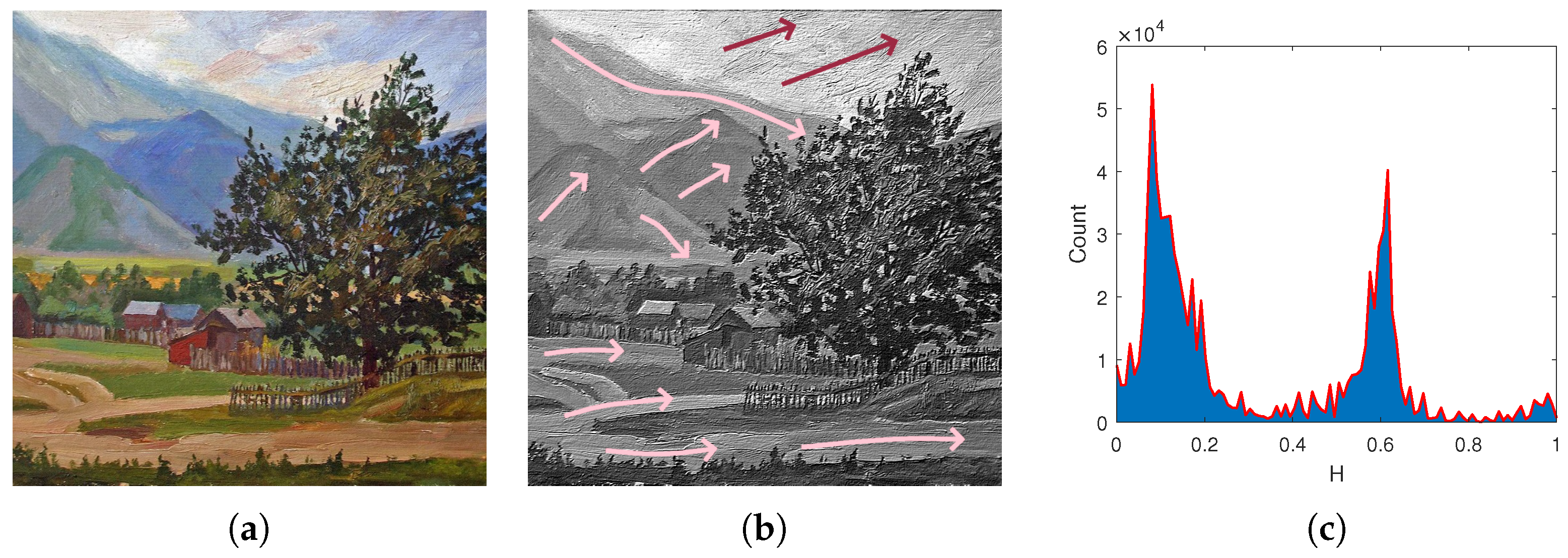
To exemplify how the proposed issues can be implemented in a real painting, we show an etude by S. Leonov given in Figure 1. The painting has a prominent aerial perspective, well-ordered brushstrokes and a specific hue histogram related to the so-called “harmonic gamut”.
In general, image preprocessing might be unnecessary in some cases, but sometimes elaborate preparation might be needed. In our paper, we propose three-stage image processing technique:
- Aerial perspective enhancement
- Gamut correction
- Averaging of the edge field extracted from the image for controlling brushstroke orientation
The image with aerial perspective enhancement, gamut correction and the edge field is then used for brushstroke rendering by the modified Herzmann’s algorithm [6].
The findings of the paper are novel computationally simple algorithms for aerial perspective enhancement, gamut correction and brushstroke coherence enhancement. They are verified via simulated artworks and a painting of a real robot.
The rest of the paper is organized as follows. Section 2 reports the description of the algorithm for aerial perspective enhancement. Section 3 is dedicated to the gamut correction. Section 4 is dedicated to the brushstroke coherence control. Experimental results are presented in Section 5. The conclusions follow in Section 6.
2. Aerial Perspective Enhancement
2.1. Related Work
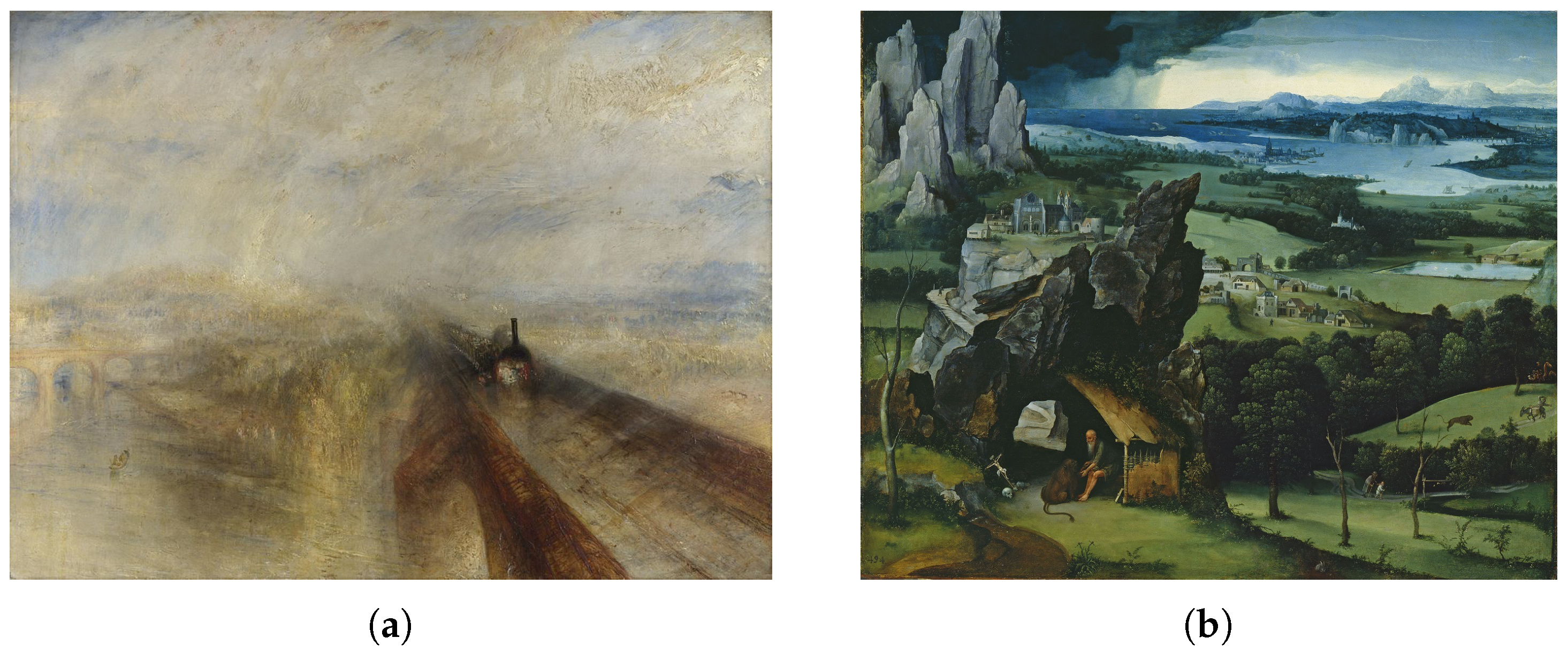
Aerial perspective together with linear perspective comprises one of the two main ways to create an illusion of depth in paintings. It was known since early periods of visual art: examples of aerial perspective are discovered in ancient Greco-Roman wall paintings [21]. In modern figurative art, it plays an important role, providing a way to distinguish overlapped close objects and define the distance to the further objects and figures in 2D image space. Enhancement of aerial perspective improves the artistic impression, examples of which can be found in artworks of many famous artists. Two prominent examples are given in Figure 2.
The examples of aerial perspective may be found even in still lifes when closer objects are intentionally painted with more bright and saturated colors.
In technical applications, atmospheric perspective in photographs caused by air turbidity, mist, dust and smoke is often undesirable because it decreases the contrast of distant objects and makes the image processing difficult [22]. Several techniques have been proposed to reduce haze, including heuristic approaches [22] and physics-based approaches [23]. In the latter work, Narasimhan and Nayar adopted the exponential model of light scattering, also used for aerial perspective rendering [24] in mixed reality applications. Following this approach, we develop an algorithm for aerial perspective enhancement in painterly rendering application.
Artificial aerial perspective may not only be used for artistic purposes but for some technical applications as well. For example, Raskar et al. used a special camera and an image processing algorithm for rendering technical sketches with artificially enhanced contours [25]. The artificial aerial perspective does not introduce additional lines and details into an image and can be useful in some cases: for example, when there are too many lines and small details in the original image, and adding contours would make the image messy and poorly readable.
2.2. Synthetic Aerial Perspective
The exponential model of light scattering is described by the equation
where is the atmospheric scattering coefficient, s is the distance to the object, is the light coming from the object directly, is the light from the infinite background (atmospheric light) and L is the apparent color of the object as perceived by the observer. For the images in RGB colorspace, Equation (1) may be applied to every color channel of each pixel. To determine the distance s, one should use the depth map, which can be obtained using various methods, including 3D scanning approaches [26], artificial intelligence methods [27], atmospheric transparency estimation [23] or constructed manually.
To obtain the coefficient for the real-world scene, air turbidity may be estimated experimentally [24]. For our purposes, one does not need an accurate value of this parameter.
Let us propose a simple method for controlling apparent air transparency. First, we should recall that depth maps are often represented with grayscale images where lighter color refers to closer objects [26,28]. Denote the minimal and maximal values in the depth map as and . Taking d as the depth map pixel brightness, the actual computational formula for aerial perspective derived from (1) is given by:
To compute the scattering parameter , we introduce a control parameter a in range . The value 0 corresponds to ideally transparent air and 1 corresponds to the case . Thus, from (2), we obtain a formula for parameter estimation:
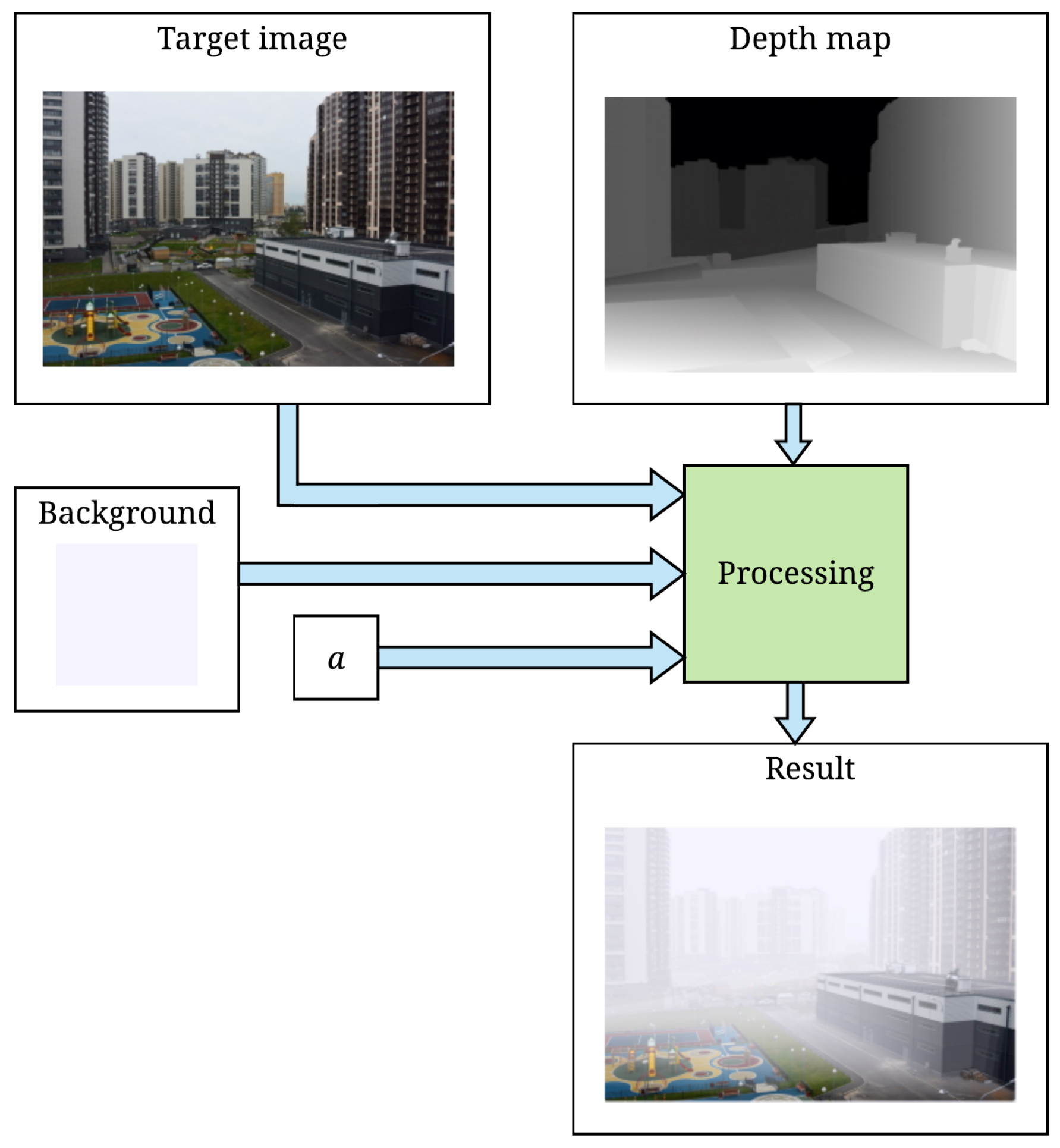
It is possible to render the aerial perspective in an arbitrary scene without connection with real air transparency using this approach. The main condition for obtaining consistent results is using a noiseless and continuous depth map without regions with undefined distances. In Section 5, we render the test images using both real and manually constructed depth maps and show that the visual effect is similar even when the depth is estimated inaccurately, in the case of manually constructed depth maps. The process is described graphically in Figure 3. Input data include source image, depth map, background color and the attenuation coefficient a. These parameters are set by the user. Using Equation (2), the colors of the background and the target image are mixed in proportions controlled by the depth map and the attenuation coefficient.
3. Gamut Correction
3.1. Related Work
Methods for controlling the gamut of the image are useful not only in non-photorealistic rendering but in artistic photography and technical applications as well. The basics of modifying the gamut are described in [12]. Organizing color scheme in a way artists do [11,14,29] may sufficiently enhance the artistic perception of the work and make the robotic painting look closer to real artworks. To perform the gamut correction, several techniques have been proposed. One of the most advanced techniques called “color harmonization” was described by Cohen-Or et al. [29]. The proposed “color harmonization” algorithm optimizes the H channel values of the image in HSV color space to fit one of the pre-defined color templates, compressing the hue histogram into two unequal sectors on opposite sides of the color wheel. The simple linear compression law for this purpose is
where C is the central hue in the color wheel sector, corresponding to a harmonic template, is the hue of the original image pixel, is the length of the arc on the uncompressed color wheel, and w is the length of the color wheel sector, corresponding to a harmonic template. Cohen-Or et al. [29] proposed a more elaborate scheme, implying that the hue update law is nonlinear and smoother than (4):
In (5), is the normalized Gaussian function with mean 0 and standard deviation . It has been proposed to optimize a special cost function referring to the error between the original histogram and one of the pre-defined harmonic schemes and updating the pixel values with the law (4) or (5).
The disadvantage of this method is that the rendered hue transformation is discontinuous, which leads to artifacts in the resulting image and unnatural hue histogram shape. To avoid these artifacts, semantic image information or manual correction is needed.
3.2. Continuous Gamut Correction
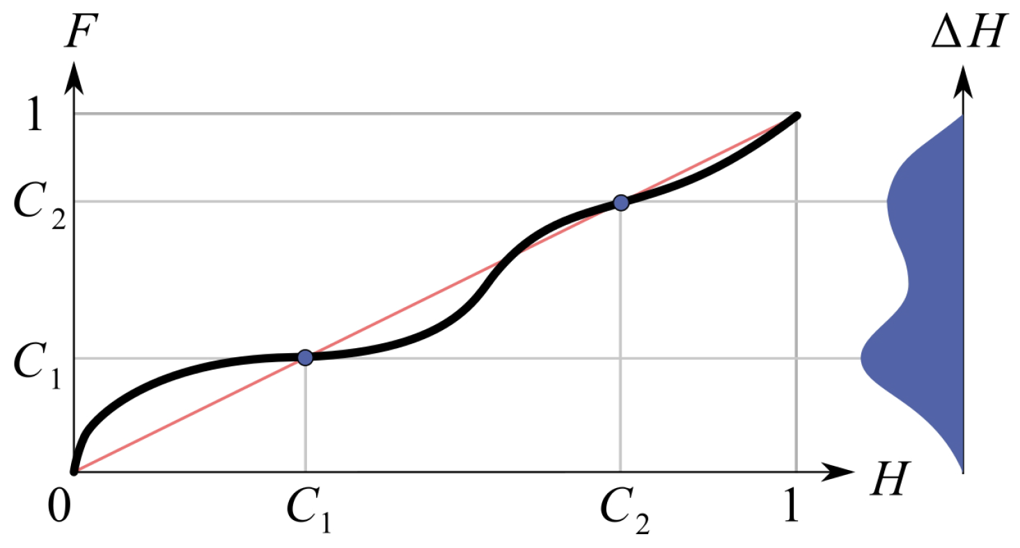
The more natural way is to construct a smooth or piecewise linear function with a small slope by values where k is the number of desired resulting histogram peaks, usually from 1 to 3, and a steep slope near intermediate hues. The possible plot of this function is given in Figure 4.
Several functions have the desired properties, for example, or any other type of sigmoid functions, but the most versatile way for designing and controlling the function is using piecewise linear, polynomial or spline approximations, e.g., the Newton polynomials. Figure 4 illustrates how the shape of the function modifies the histogram, where the plot for gives the difference between the original hue histogram and the resulting histogram . The red line in Figure 4 refers to the identity , which has no impact on the histogram.
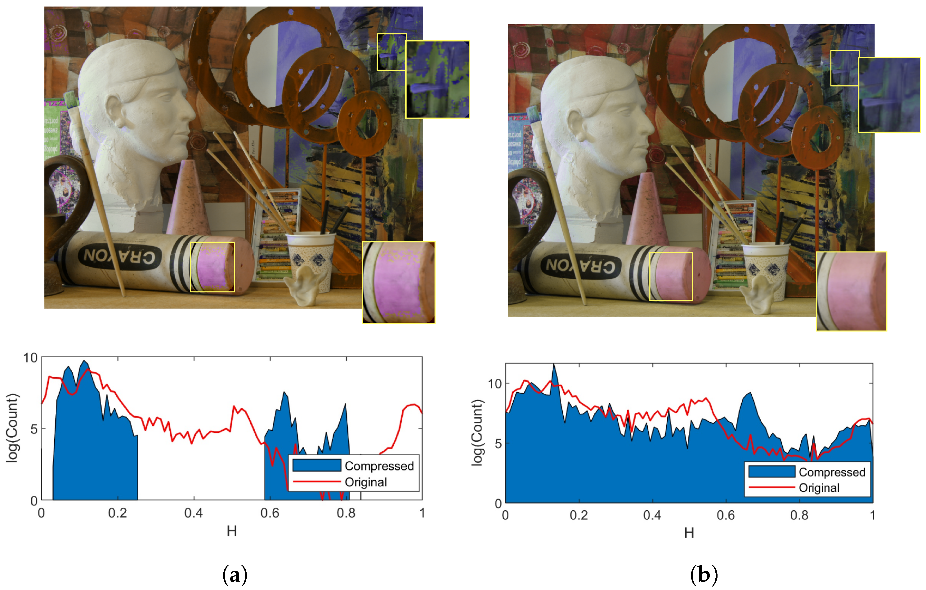
Figure 5 presents the results obtained by the “color harmonization” approach and the proposed technique on the test image “Art” [26]. We used this image because it is a part of the test set for stereo matching algorithms and has a reliable depth map obtained by 3D scanning. Artifacts in the image after color harmonization are given in boxes, while the same regions of the picture preserve natural view when the continuous compression function is applied. The second notable difference is that the hue histogram after harmonization by templates becomes discontinuous, which looks unnatural and can affect the perception of a scene.
In our work, we use a piecewise-linear function composed of n pieces, determined as follows
where are user-defined points and and are bounds of pieces. We use pieces, which is sufficient for almost any gamut correction task.
In Section 5, the results for several test images are given proving that the proposed approach is fruitful and more efficient than “color harmonization”.
4. Brushstroke Coherence Control
4.1. Related Work
Herzmann’s algorithm is probably the most popular algorithm for brushstroke computation [9,17,30,31]. It uses a special edge field projected on the image for controlling brushstroke orientation. It generates long curved brushstrokes using the following scheme.
First, seed points are placed onto an image. Then, from each seed point, a brushstroke grows by segments so that each segment starting from an image point is oriented in accordance with the local orientation of the edge field . For example, when the gradient vector field is used as the edge field, each segment is oriented normally to the local gradient. The brushstroke stops growing when its color stops fitting the underlying source image color or its length exceeds a predefined maximal value. The algorithm finishes when all seed points have been involved.
Herzmann’s algorithm can be easily adapted for using multiple brush sizes and shapes. Since a physical set of brushstrokes is computed, the algorithm is more computationally expensive in comparison with some other non-photorealistic rendering approaches without brushstroke simulation, e.g., coherence-enhancing filtering [32]. The original version of Herzmann’s algorithm allows computing each brushstroke independently and can be parallelized on GPU in a manner proposed by Meier [33] or Umenhoffer et al. [34].
Nevertheless, actual issues in the robotic painting are tended to reduce the number of brushstrokes while retaining dense canvas covering and a predefined brushstroke application order (in our work, it is from dark to light). Generating the next brushstroke needs keeping in mind previously computed ones and therefore parallelization is difficult [9]. Another problem of this painterly rendering approach is that, even if some extra conditions on brushstroke mutual orientation are imposed, the brushstroke orientation remains unnaturally stochastic if the edge field computed from the image is not sufficiently smooth. Thus, special edge field control schemes are required. Before considering them, recall how the edge field is computed.
The first kind of edge fields for controlling brushstroke orientation is the vector-based edge field extracted from the image using numerical differentiation operator [8,17,19]. For example, the Sobel operator can be used for gradient estimation:
The more advanced way to compute gradient is using the rotational symmetric derivative operator [35]
where .
The more elaborate technique for the edge field design is constructing a structure tensor field [32]. The structure tensor components are composed from scalar products of gradients:
The major and minor eigenvalues are then found from the relation:
The corresponding major and minor eigenvectors are:
The major eigenvector points towards the direction of maximum change, while the minor eigenvector is orthogonal to it and shows the direction of maximum uniformity. Major eigenvectors can be used instead of the gradient to control the brushstroke orientation using the tensor-based edge field.
In practice, numerical differentiation is usually undesired since it amplifies noise. When the gradient is computed from the image, even small noise can lead to a sufficient incoherence of the extracted gradient vectors. One of the possible ways to decrease this effect is filtering matrices and C from (9) using Gaussian or any other type of smoothing filters [32]. This operation can also be represented as a convolution with Gaussian matrix G: , where M is a target matrix and is the smoothed matrix. Filtering may suppress artifacts caused by the noise, but it still does not necessarily provide good brushstroke coherence in practical cases. The reason is that images often contain many almost uniform regions where the gradient magnitude is low and numerical gradient computation algorithms do not provide reliable results. A possible solution to this problem is replacing tensors with major eigenvector magnitude lower than a threshold using interpolation between neighboring vectors [32]. This causes discontinuities near borders of regions with a magnitude lower and greater than , and a large number of iterations is needed to achieve appropriate smoothing.
Another way to improve the edge field is the interaction with the user. For example, Zhang et al. proposed an interactive tool for tensor field manual correction by editing tensor field degenerate points [19]. Igno et al. developed an approach based on the natural neighbor interpolation between manually drawn splines following the depicted scene features such as object edges and generatrices [20]. These approaches allow utilizing semantic information accessible to the user and rendering the painting more accurately.
4.2. Coherence Enhancement by Averaging
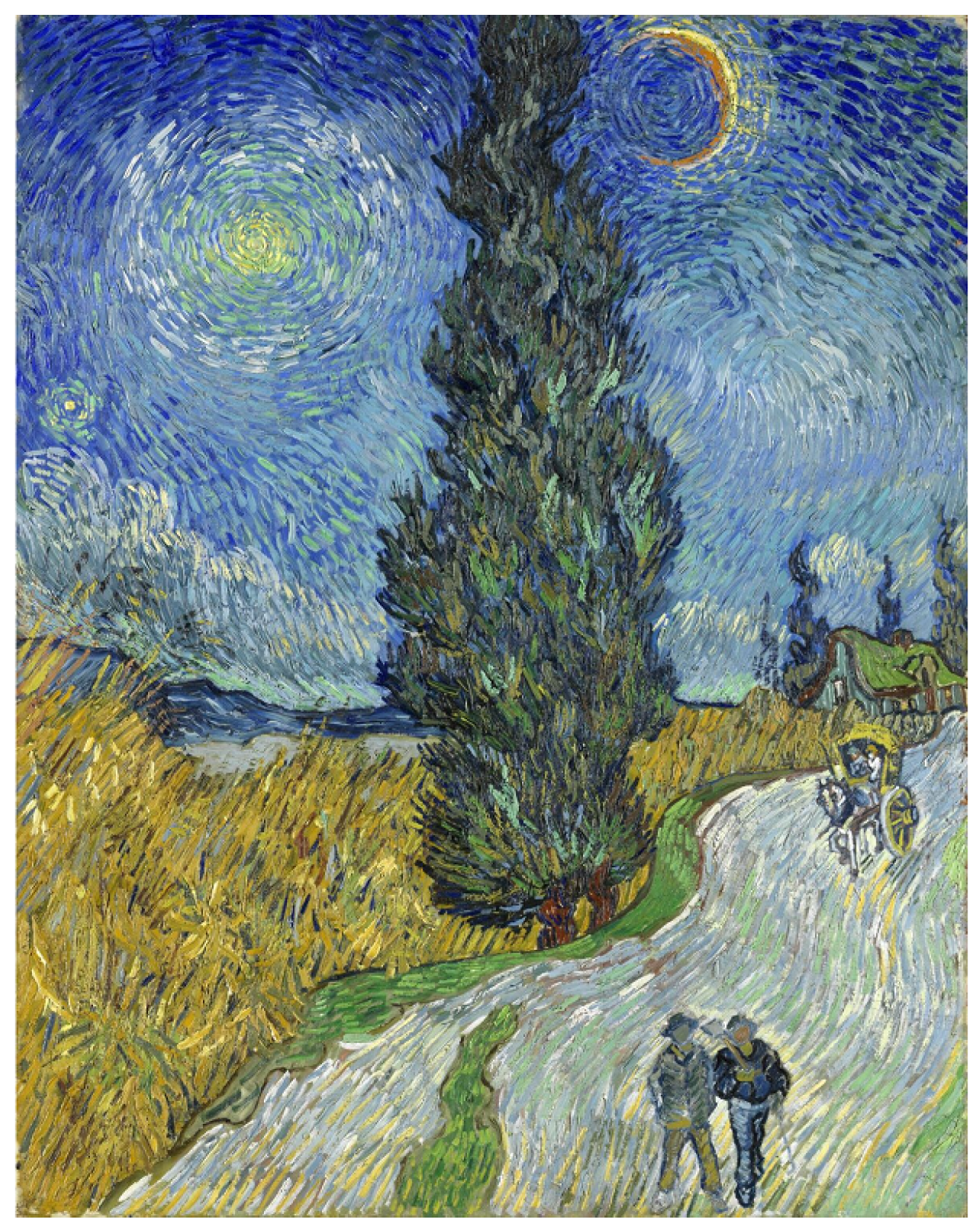
In this work, we propose an automatic coherence enhancement method by averaging. It is based on the observation that the magnitude of eigenvectors on edges or other sufficiently heterogeneous image regions computed by Equations (7)–(11) is notably higher than in nearly uniform regions where these operators give unreliable results. Therefore, linear spatial averaging of x and y vector components will usually preserve the orientation of vectors with large magnitude and suppress erroneous direction components in vectors with small magnitude. This idea is consonant with the artistic painting technique used by many artists when the brushstrokes follow the orientation of edges in the depicted scene. An example of this artistic technique is given in Figure 6.
We use the averaging filter with matrix
Let U and V be matrices of x and y major eigenvector (10) components, respectively, and an edge field is the projection of the tensor field S on the image. The averaging matrix (12) is then convolved with U and V in order to produce smoothened edge field , where
The size m of the matrix W is selected with respect to the brush radius R. Reasonable results are achieved with values . The value can be recommended for the first test on any image, and the values over provide an extremely smoothed brushstroke map which is likely to ignore many local features of the image.
Summarizing, the following coherence enhancement algorithm is proposed (in Algorithm 1):
| Algorithm 1: Obtaining a smoothed edge field from an image |
| input: a bitmap , parameters of matrices output: a vector field Fs // Load a bitmap I ← LoadImage ; // Find derivatives Fx ← ∗ I ; Fy ← ∗ I ; A ← Fx · Fx, B ← Fx · Fy, C ← Fy · Fy ; // Convolve with the Gaussian matrix and processing the tensor field A ← G ∗ A, B ← G ∗ B, C ← G ∗ C ; S ← GetTensorField (A, B, C) [U,V ] ← GetMajorEigenvectors (S); // Convolve with the averaging matrix U ← W ∗ U ; V ← W ∗ V ; // Obtain the final result Fs ← [U, V ]; |
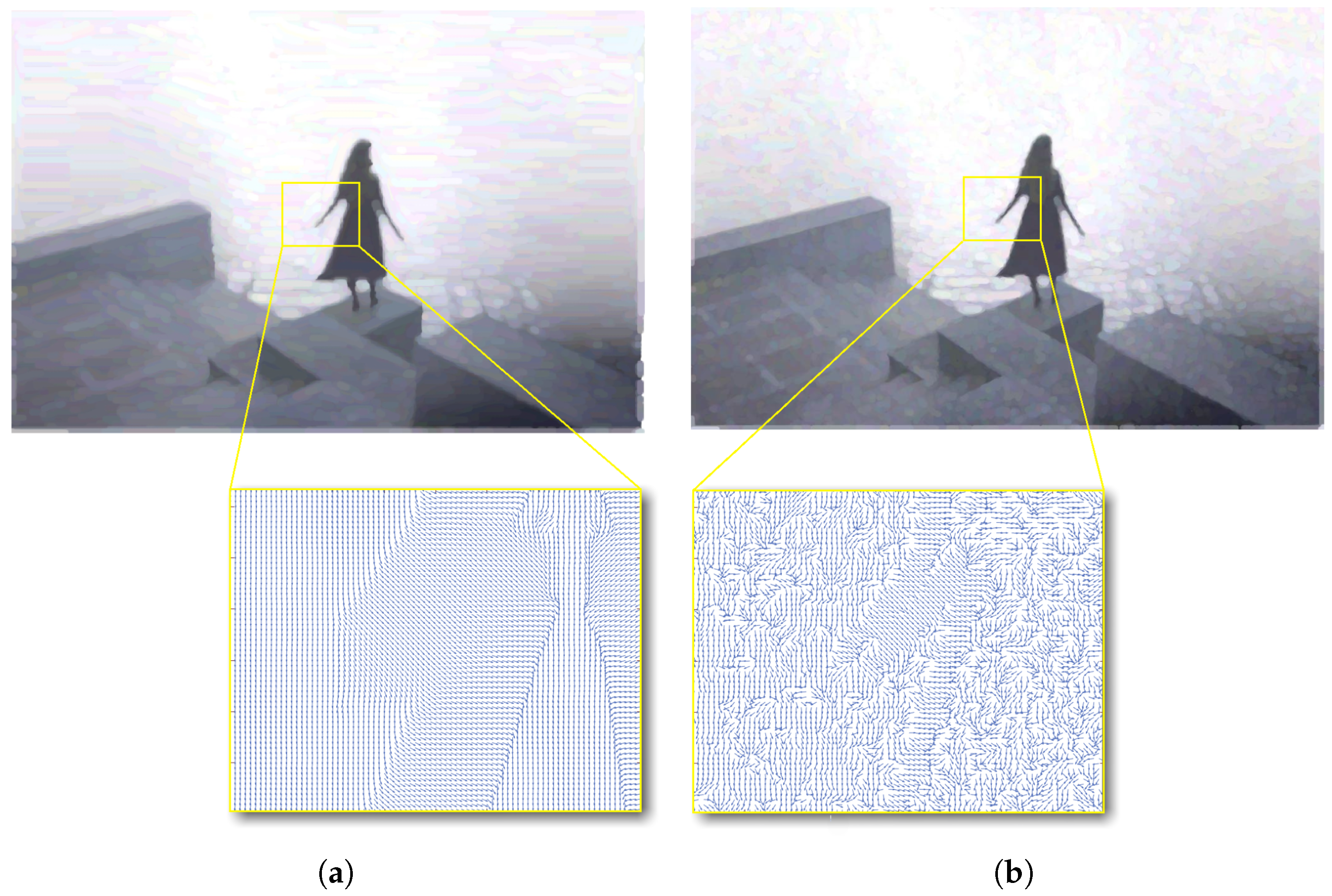
Figure 7 shows the results of the proposed approach in comparison with the results based on Gaussian filtering of and C components of S in (9) only. To obtain brushstroke maps, an algorithm from Karimov et al. [9] was used. Notice the regular behavior of brushstrokes in the image obtained by the proposed approach. The value was used. The brushstrokes in Figure 7b are notably more irregular than in Figure 7a.
5. Experimental Results
In this section, we illustrate the stages of image preprocessing and present some of the results.
5.1. Experiments with Simulated Painting
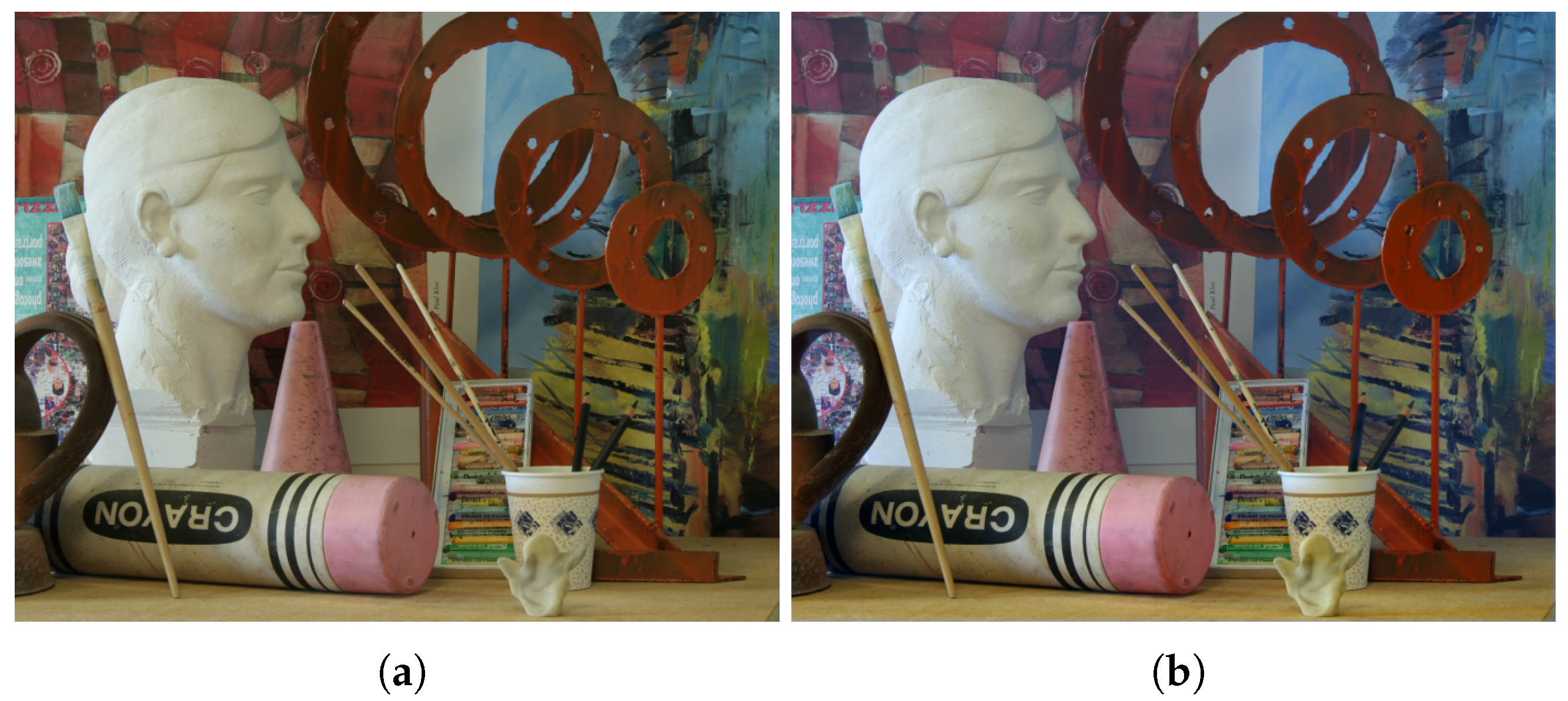
First, let us illustrate how aerial perspective can improve the image depth perception. In the first experiment, we used the “Art” test image for rendering the aerial perspective and enhanced the apparent depth of this still life. Using the provided depth map, we rendered the aerial perspective using light-blue infinite background and the value of attenuation parameter . To eliminate some artifacts contained in the depth map, the original depth map was first filtered with a histogram filter to cut off of the rarest distance values and thus remove artifacts from the depth map, and then blurred with Gaussian filter of size with . Figure 8a shows the original image and Figure 8b shows a resulting image with an aerial perspective. Objects became more distinguishable from the background and each other. The brushstroke rendering results are not shown here.
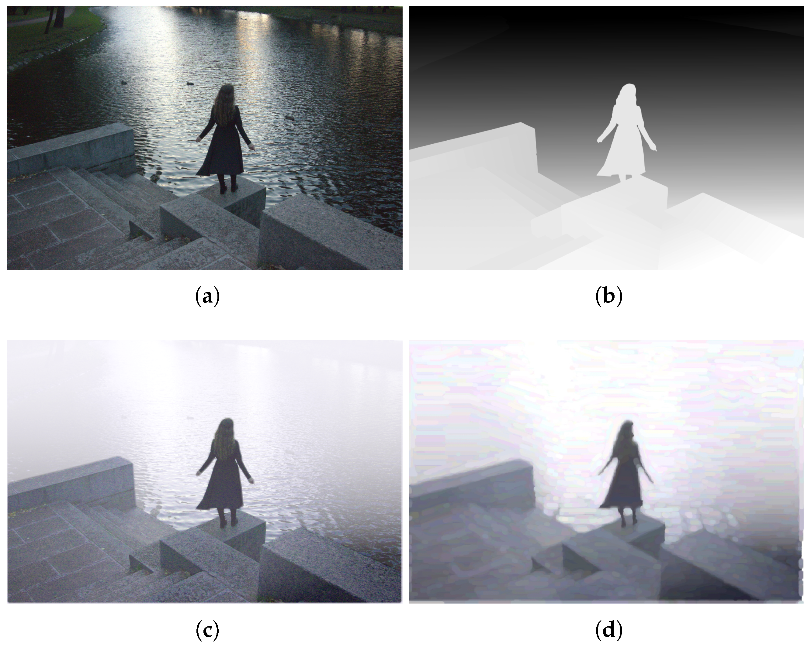
Second, we show that a manually painted depth map does not affect the final image quality. Figure 9a shows a photograph taken in normal air conditions. Suppose an artist inspired by Turner’s “Rain, Steam and Speed” wants to obtain a similar effect. The depth map shown in Figure 9b was constructed manually using the source image, and all distances were estimated approximately. The aerial perspective enhancement leads to an effect of mist, as shown in Figure 9c, an infinite background color was chosen close to white and the attenuation parameter was set . The rendering result is presented in Figure 9d, which is similar to Figure 7a. Averaging also results in the economy of brushstrokes: the render contains 25,865 brushstrokes without coherence enhancement and 24,191 brushstrokes with coherence enhancement, which comprises approximately reduction.
5.2. Experiments with the Robotic Painting
Our experimental robot ARTCYBE is currently capable of monochromatic painting with acrylic paints. It is a three degrees of freedom gantry robot with a working area of 50 cm × 70 cm. It has a block of syringe pumps and a brush as an end effector. The working cycle of the robot starts from injecting fluid acrylic paints into a small paint mixer in a required proportion. An impeller inside the mixer starts rotating and preparing the mixture of the required tint. Then, the robot starts painting brushstrokes of the required tint, extruding the paint from its hollow brush onto a canvas. When the paint ends, it renews the paint mixture. After all strokes of the current tint are painted, it washes the mixer and the brush and proceeds with the next tint. More details of the robot design and its main technical characteristics can be found in [6].
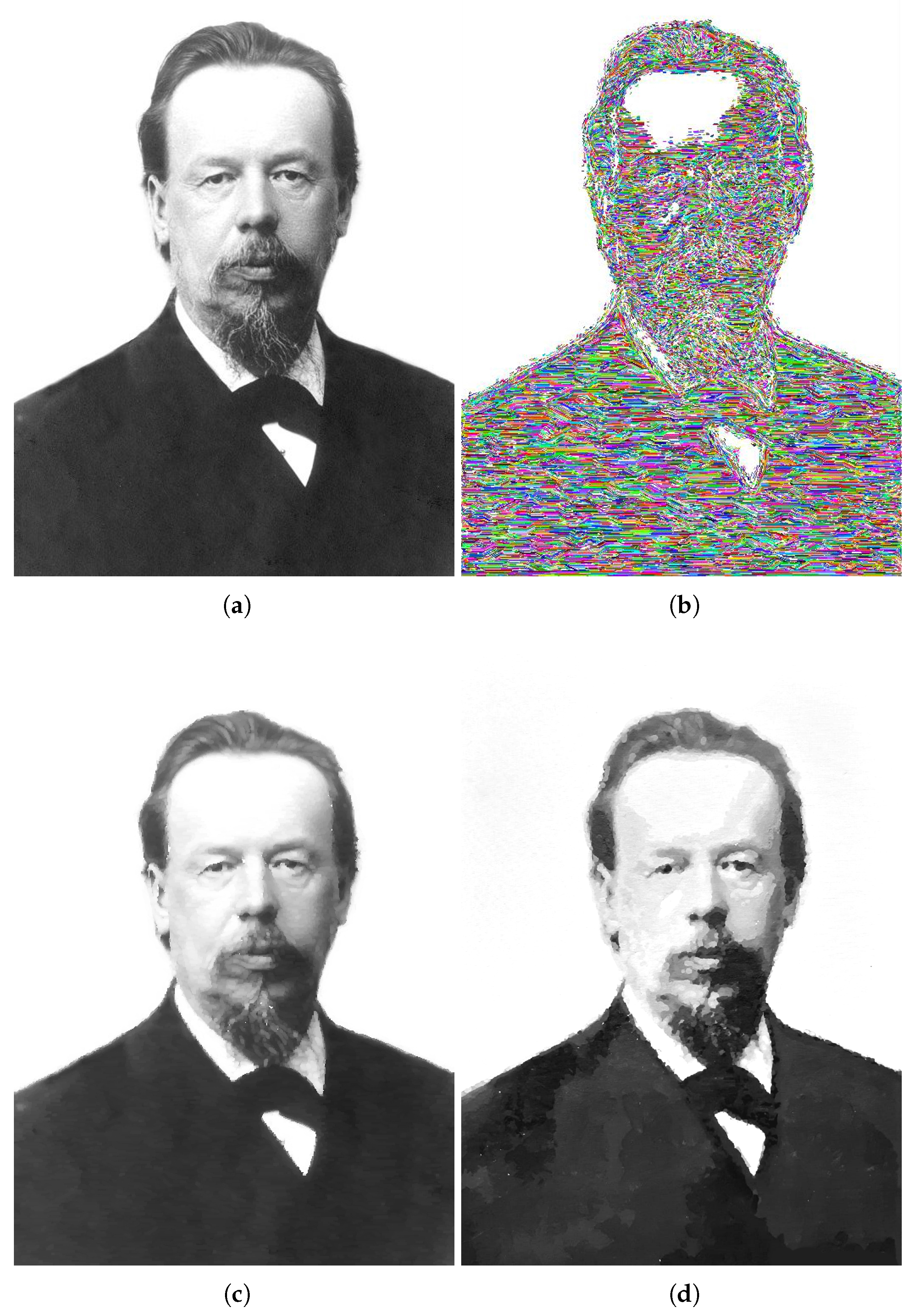
Since the current version of the robot can implement only monochromatic images, the full-scale test with this machine can be performed only with coherence enhancement, because aerial perspective and especially gamut correction require color painting. In this experiment, we render the photo of Aleksandr Popov, known as the inventor of the radio (along with G. Marconi) and the first elected rector of ETU “LETI”. The source image has a size 520 × 706 pixels. The coherence enhancement allows reducing the number of strokes from 35,028 strokes to 33,175 strokes, when the averaging filer with is used, which comprises brushstroke number reduction. Moreover, without coherence enhancement, the generated strokes are fairly stochastic due to the noise in the source image. Figure 11 presents four stages of image processing.
Let us consider the stages of image processing in detail. First, the source image given in Figure 11a is manually corrected to obtain a permanently white background. This sufficiently reduces the required amount of paint needed to cover the canvas covered with the white primer. Next, the brushstroke map (Figure 11b) and the render (Figure 11c) are generated. In Figure 11b, it is clearly seen that uniform regions are rendered with long horizontal strokes. Finally, the painting is implemented on canvas (Figure 11d).
In this experiment, we use 50 cm × 70 cm canvas on cardboard and specially prepared acrylic paints manufactured by a local brand “Nevskaya palitra”. Due to some limitations in tone rendition accuracy, the final image in Figure 11d has slightly fewer tone grades than the render in Figure 11c, but the brushstroke shapes are implemented accurately.
6. Conclusions and Discussion
Image preprocessing for artistic painterly rendering is a non-trivial task since there is no general recipe for how a human artist converts the visual perception into a painting. Our work is based on several principles and traditions in art and proposes three special image processing techniques for making the image look more artistically impressive.
Tests with simulated images and an artistically skilled robot show the applicability of the proposed approaches. We show that the enhanced aerial perspective can increase the image perceived depth; the proposed gamut correction approach allows exact and continuous hue transformation for better artistic impression; and the brushstroke coherence enhancement approach makes the rendered image more orderly and reduces the number of brushstrokes, which results in better painting quality and less working time of the robot.
While we show the benefits of these methods by examples, additional investigation is needed to unveil how these algorithms were implicitly used by artists through the years. Thus, the future work will be focused on "reverse engineering" of these painting techniques from a large database of artistic images with the use of machine learning and artificial intelligence. First, it is of interest to find which characteristics of aerial perspective are most common in arts. Second, one can find an optimal shape of hue correction function after analyzing a certain number of artworks. Third, one can analyze strokes of particular artists and find an optimal algorithm for brushstroke coherence control and imitate the individual style of the artist. For example, van Gogh’s style of highly coherent brushstrokes is of a notable interest [36].
It is also important to compare artificial intuition and artificial creativity as two related branches of artificial intelligence and denote the role of the current work in these fields. As usually emphasized by artists who belong to the traditional realistic schools, technical skills are not less important than personal manner and emotions. Today, it is not entirely clear what makes us feel strong emotions from one painting and remain indifferent to another, even technically more perfect. However, undoubtedly, limited artist’s skills can spoil even a brilliant idea. Artists spend a lot of time to achieve a high technical level but usually have no problems with creativity and transmitting their message to viewers. As for machines, today, they are technically more skilled than human artists in many aspects. Only a few technical problems remain unresolved in machine painting such as performing colored oil painting. However, it is important to note that what we call “intuition” is still a matter of speculations. For example, recent advances with GANs such as StyleGAN2 [37] show that these algorithms can already generate high-grade original images. However, roughly speaking, they combine various fragments of images in beautiful but meaningless combinations and cannot go beyond the boundaries of the style of artists on whose paintings they were trained. Thus, the vector of artificial intelligence development is directed to the technical side of creativity rather than to improving artificial intuition, and this paper also contributes to the technical aspect of the issue.
Author Contributions
Conceptualization, A.K. and S.L.; data curation, A.K. and G.K.; formal analysis, S.L. and D.B.; investigation, A.K., E.K. and D.B.; methodology, A.K., L.S. and D.B.; project administration, A.K. and D.B.; resources, A.K., E.K., S.L. and L.S.; software, A.K., E.K. and G.K.; supervision, S.L. and D.B.; validation, G.K. and L.S.; visualization, A.K., E.K. and G.K.; writing—original draft, A.K. and D.B.; and writing—review and editing, L.S. and D.B. All authors have read and agreed to the published version of the manuscript.
Funding
This research received no external funding.
Institutional Review Board Statement
Not applicable.
Informed Consent Statement
Not applicable.
Conflicts of Interest
The authors declare no conflict of interest.
References
- Cohen, H. How to Draw Three People in a Botanical Garden; AAAI: Menlo Park, CA, USA, 1988; Volume 89, pp. 846–855. [Google Scholar]
- Avila, L.; Bailey, M. Art in the digital age. IEEE Comput. Graph. Appl. 2016, 36, 6–7. [Google Scholar]
- Scalera, L.; Seriani, S.; Gasparetto, A.; Gallina, P. Non-photorealistic rendering techniques for artistic robotic painting. Robotics 2019, 8, 10. [Google Scholar] [CrossRef] [Green Version]
- Gülzow, J.; Grayver, L.; Deussen, O. Self-improving robotic brushstroke replication. Arts 2018, 7, 84. [Google Scholar] [CrossRef] [Green Version]
- Scalera, L.; Seriani, S.; Gasparetto, A.; Gallina, P. Watercolour robotic painting: A novel automatic system for artistic rendering. J. Intell. Robot. Syst. 2019, 95, 871–886. [Google Scholar] [CrossRef]
- Karimov, A.I.; Kopets, E.E.; Rybin, V.G.; Leonov, S.V.; Voroshilova, A.I.; Butusov, D.N. Advanced tone rendition technique for a painting robot. Robot. Auton. Syst. 2019, 115, 17–27. [Google Scholar] [CrossRef]
- Shiraishi, M.; Yamaguchi, Y. An algorithm for automatic painterly rendering based on local source image approximation. In Proceedings of the 1st International Symposium on Non-Photorealistic Animation and Rendering, Annecy, France, 5–7 June 2000; pp. 53–58. [Google Scholar]
- Litwinowicz, P. Processing images and video for an impressionist effect. In Proceedings of the 24th Annual Conference on Computer Graphics and Interactive Techniques, New York, NY, USA, 4 August 1997; Citeseer: State College, PA, USA, 1997; pp. 407–414. [Google Scholar]
- Karimov, A.I.; Pesterev, D.O.; Ostrovskii, V.Y.; Butusov, D.N.; Kopets, E.E. Brushstroke rendering algorithm for a painting robot. In Proceedings of the 2017 International Conference “Quality Management, Transport and Information Security, Information Technologies” (IT&QM&IS), St. Petersburg, Rusia, 24–30 September 2017; pp. 331–334. [Google Scholar]
- Vanderhaeghe, D.; Collomosse, J. Stroke based painterly rendering. In Image and Video-Based Artistic Stylisation; Springer: London, UK, 2013; pp. 3–21. [Google Scholar]
- Zang, Y.; Huang, H.; Li, C.F. Artistic preprocessing for painterly rendering and image stylization. Vis. Comput. 2014, 30, 969–979. [Google Scholar] [CrossRef]
- Morovic, J.; Luo, M.R. The fundamentals of gamut mapping: A survey. J. Imaging Sci. Technol. 2001, 45, 283–290. [Google Scholar]
- Ames, A., Jr. Depth in pictorial art. Art Bull. 1925, 8, 5–24. [Google Scholar] [CrossRef]
- Kim, D.; Son, S.W.; Jeong, H. Large-scale quantitative analysis of painting arts. Sci. Rep. 2014, 4, 7370. [Google Scholar] [CrossRef] [Green Version]
- Zeng, K.; Zhao, M.; Xiong, C.; Zhu, S.C. From image parsing to painterly rendering. ACM Trans. Graph. 2009, 29, 2–11. [Google Scholar] [CrossRef]
- Cotte, P.; Dupraz, D. Spectral imaging of Leonardo Da Vinci’s Mona Lisa: A true color smile without the influence of aged varnish. In Proceedings of the Conference on Colour in Graphics, Imaging, and Vision. Society for Imaging Science and Technology, Leeds, UK, 19–22 June 2006; Volume 2006, pp. 311–317. [Google Scholar]
- Hertzmann, A. A survey of stroke-based rendering. IEEE Comput. Graph. Appl. 2003, 70–81. [Google Scholar] [CrossRef] [Green Version]
- Rosin, P.; Collomosse, J. Image and Video-Based Artistic Stylisation; Springer Science & Business Media: Berlin/Heidelberg, Germany, 2012; Volume 42. [Google Scholar]
- Zhang, E.; Hays, J.; Turk, G. Interactive tensor field design and visualization on surfaces. IEEE Trans. Vis. Comput. Graph. 2006, 13, 94–107. [Google Scholar] [CrossRef] [Green Version]
- Igno-Rosario, O.; Hernandez-Aguilar, C.; Cruz-Orea, A.; Dominguez-Pacheco, A. Interactive system for painting artworks by regions using a robot. Robot. Auton. Syst. 2019, 121, 103263. [Google Scholar] [CrossRef]
- Messina, B.; Pascariello Ines, M. The architectural perspectives in the villa of Oplontis, a space over the real. In Proceedings of the Le vie dei Mercanti XIII International Forum, Aversa, Capri, Italy, 11–13 June 2015. [Google Scholar]
- He, K.; Sun, J.; Tang, X. Single image haze removal using dark channel prior. IEEE Trans. Pattern Anal. Mach. Intell. 2010, 33, 2341–2353. [Google Scholar] [PubMed]
- Narasimhan, S.G.; Nayar, S.K. Contrast restoration of weather degraded images. IEEE Trans. Pattern Anal. Mach. Intell. 2003, 25, 713–724. [Google Scholar] [CrossRef] [Green Version]
- Morales, C.; Oishi, T.; Ikeuchi, K. Real-time rendering of aerial perspective effect based on turbidity estimation. IPSJ Trans. Comput. Vis. Appl. 2017, 9, 1. [Google Scholar] [CrossRef] [Green Version]
- Raskar, R.; Tan, K.H.; Feris, R.; Yu, J.; Turk, M. Non-photorealistic camera: Depth edge detection and stylized rendering using multi-flash imaging. ACM Trans. Graph. (TOG) 2004, 23, 679–688. [Google Scholar] [CrossRef]
- Hirschmuller, H.; Scharstein, D. Evaluation of cost functions for stereo matching. In Proceedings of the 2007 IEEE Conference on Computer Vision and Pattern Recognition, Minneapolis, MN, USA, 17–22 June 2007; pp. 1–8. [Google Scholar]
- Eigen, D.; Puhrsch, C.; Fergus, R. Depth map prediction from a single image using a multi-scale deep network. In Advances in Neural Information Processing Systems; MIT Press: Cambridge, MA, USA, 2014; pp. 2366–2374. [Google Scholar]
- Peris, M.; Martull, S.; Maki, A.; Ohkawa, Y.; Fukui, K. Towards a simulation driven stereo vision system. In Proceedings of the 21st International Conference on Pattern Recognition (ICPR2012), Tsukuba, Japan, 11–15 November 2012; pp. 1038–1042. [Google Scholar]
- Cohen-Or, D.; Sorkine, O.; Gal, R.; Leyvand, T.; Xu, Y.Q. Color harmonization. ACM Trans. Graph. (TOG) 2006, 25, 624–630. [Google Scholar] [CrossRef]
- Hertzmann, A. Painterly rendering with curved brush strokes of multiple sizes. In Proceedings of the 25th Annual Conference on Computer Graphics and Interactive Techniques, Orlando, FL, USA, 19–24 July 1998; ACM: New York, NY, USA, 1998; pp. 453–460. [Google Scholar]
- Hegde, S.; Gatzidis, C.; Tian, F. Painterly rendering techniques: A state-of-the-art review of current approaches. Comput. Animat. Virtual Worlds 2013, 24, 43–64. [Google Scholar] [CrossRef]
- Kyprianidis, J.E.; Kang, H. Image and video abstraction by coherence-enhancing filtering. In Computer Graphics Forum; Wiley Online Library: Hoboken, NJ, USA, 2011; Volume 30, pp. 593–602. [Google Scholar]
- Meier, B.J. Painterly rendering for animation. In Proceedings of the 23rd Annual Conference on Computer Graphics and Interactive Techniques, New Orleans, LA, USA, 4–9 August 1996; Citeseer: State College, PA, USA, 1996; pp. 477–484. [Google Scholar]
- Umenhoffer, T.; Szirmay-Kalos, L.; Szécsi, L.; Lengyel, Z.; Marinov, G. An image-based method for animated stroke rendering. Vis. Comput. 2018, 34, 817–827. [Google Scholar] [CrossRef]
- Jähne, B.; Scharr, H.; Körkel, S. Principles of filter design. Handb. Comput. Vis. Appl. 1999, 2, 125–151. [Google Scholar]
- Li, J.; Yao, L.; Hendriks, E.; Wang, J.Z. Rhythmic brushstrokes distinguish van Gogh from his contemporaries: Findings via automated brushstroke extraction. IEEE Trans. Pattern Anal. Mach. Intell. 2011, 34, 1159–1176. [Google Scholar]
- Karras, T.; Aittala, M.; Hellsten, J.; Laine, S.; Lehtinen, J.; Aila, T. Training generative adversarial networks with limited data. arXiv 2020, arXiv:2006.06676. [Google Scholar]
Figure 1.
(a) The original image. It has a blue pale background due to aerial perspective. (b) The predominant directions of brushstrokes in some regions of the image. In these regions, the brushstrokes are highly coherent. (c) The hue histogram showing that it has two distinct peaks near complementary colors: orange and blue .

Figure 2.
(a) An example of highly enhanced aerial perspective in art: “Rain, Steam and Speed” by J.M.W. Turner, 1844. (b) A piece where aerial perspective is rendered through bluish gamut: “Paisaje con san Jerónimo” by Joachim Patinir, 1515–1519.
Figure 2.
(a) An example of highly enhanced aerial perspective in art: “Rain, Steam and Speed” by J.M.W. Turner, 1844. (b) A piece where aerial perspective is rendered through bluish gamut: “Paisaje con san Jerónimo” by Joachim Patinir, 1515–1519.

Figure 3.
Block diagram of the aerial perspective enhancement process.

Figure 4.
Generalization of the proposed hue modification function: regions with small slope provide histogram compression by the desired peaks and , while continuity of the function in regions with steep slope ensures continuity of the modified histogram. Here, Bezier spline was used for the illustration.

Figure 5.
Gamut correction methods: color harmonization by templates (a); and the proposed method of nonlinear compression (b).
Figure 5.
Gamut correction methods: color harmonization by templates (a); and the proposed method of nonlinear compression (b).

Figure 6.
“Country road in Provence by night” by Vincent van Gogh, 1890. Painterly brushstrokes on the road follow its edges, while brushstrokes in the sky are parallel to edges of the star and the crescent.
Figure 6.
“Country road in Provence by night” by Vincent van Gogh, 1890. Painterly brushstrokes on the road follow its edges, while brushstrokes in the sky are parallel to edges of the star and the crescent.

Figure 7.
Edge field improvement by averaging: (a) a painterly rendered image using a smoothened edge field by the proposed approach; and (b) a rendered image with no averaging. Yellow frames highlight similar fragments of rendered images and show the underlying major eigenvectors used for brushstroke generation in each case.

Figure 8.
(a) The original image, which is apparently more “flat” than the processed one in (b).

Figure 9.
Aerial perspective enhancement of the source image (a) using the manually painted depth map (b) leads to a misty image (c), which is then rendered to obtain an etude-like composition (d) painted with a thick brush.
Figure 9.
Aerial perspective enhancement of the source image (a) using the manually painted depth map (b) leads to a misty image (c), which is then rendered to obtain an etude-like composition (d) painted with a thick brush.

Figure 10.
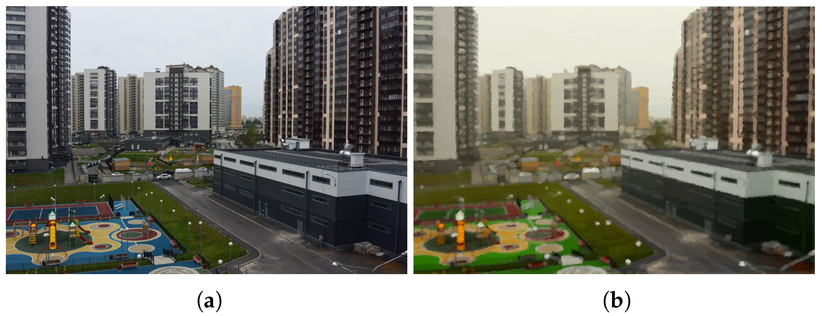
The source image (a) was processed using all four stages: aerial perspective enhancement, gamut compression for achieving an effect of yellowed old paints, contrast-saturation correction and, finally, brushstroke rendering with improved coherence. The rendering result (b) represents a simulation of generated plotter file ready for robotic artistic painting.
Figure 10.
The source image (a) was processed using all four stages: aerial perspective enhancement, gamut compression for achieving an effect of yellowed old paints, contrast-saturation correction and, finally, brushstroke rendering with improved coherence. The rendering result (b) represents a simulation of generated plotter file ready for robotic artistic painting.

Figure 11.
A slightly noisy source image (a) containing a number of monotonic areas can be rendered with well-coherent strokes generated with the technique of coherence enhancement (b). The rendered image (c) is then painted with the robot (d).
Figure 11.
A slightly noisy source image (a) containing a number of monotonic areas can be rendered with well-coherent strokes generated with the technique of coherence enhancement (b). The rendered image (c) is then painted with the robot (d).

Publisher’s Note: MDPI stays neutral with regard to jurisdictional claims in published maps and institutional affiliations. |
© 2021 by the authors. Licensee MDPI, Basel, Switzerland. This article is an open access article distributed under the terms and conditions of the Creative Commons Attribution (CC BY) license (http://creativecommons.org/licenses/by/4.0/).
Share and Cite
MDPI and ACS Style
Karimov, A.; Kopets, E.; Kolev, G.; Leonov, S.; Scalera, L.; Butusov, D. Image Preprocessing for Artistic Robotic Painting. Inventions 2021, 6, 19. https://doi.org/10.3390/inventions6010019
AMA Style
Karimov A, Kopets E, Kolev G, Leonov S, Scalera L, Butusov D. Image Preprocessing for Artistic Robotic Painting. Inventions. 2021; 6(1):19. https://doi.org/10.3390/inventions6010019
Chicago/Turabian StyleKarimov, Artur, Ekaterina Kopets, Georgii Kolev, Sergey Leonov, Lorenzo Scalera, and Denis Butusov. 2021. "Image Preprocessing for Artistic Robotic Painting" Inventions 6, no. 1: 19. https://doi.org/10.3390/inventions6010019