Storm Surge Modeling in Large Estuaries: Sensitivity Analyses to Parameters and Physical Processes in the Chesapeake Bay

Abstract

Large estuaries are especially vulnerable to coastal flooding due to the potential of combined storm surges and riverine flows. Numerical models can support flood prevention and planning for coastal communities. However, while recent advancements in the development of numerical models for storm surge prediction have led to robust and accurate models; an increasing number of parameters and physical processes’ representations are available to modelers and engineers. This study investigates uncertainties associated with the selection of physical parameters or processes involved in storm surge modeling in large estuaries. Specifically, we explored the sensitivity of a hydrodynamic model (ADCIRC) and a coupled wind-wave and circulation model system (ADCIRC + SWAN) to Manning’s n coefficient, wind waves and circulation interaction (wave setup), minimum depth (H₀) in the wetting and drying algorithm, and spatially constant horizontal eddy viscosity (ESLM) forced by tides and hurricane winds. Furthermore, sensitivity analysis to Manning’s n coefficient and the interaction of waves and circulation were analyzed by using three different numerical meshes. Manning’s coefficient analysis was divided into waterway (rivers, bay and shore, and open ocean) and overland. Overall, the rivers exhibited a larger sensitivity, and M₂ amplitude and maximum water elevations were reduced by 0.20 m and 0.56 m, respectively, by using a high friction value; similarly, high friction reduced maximum water levels up to 0.30 m in overland areas; the wave setup depended on the offshore wave height, angle of breaking, the profile morphology, and the mesh resolution, accounting for up to 0.19 m setup inside the bay; minimum depth analysis showed that H₀ = 0.01 added an artificial mass of water in marshes and channels, meanwhile H = 0.1 partially solved this problem; and the eddy viscosity study demonstrated that the ESLM = 40 values reduced up to 0.40 m the peak of the maximum water levels in the upper side of narrow rivers.

1. Introduction

Storm surge is one of the major hazards impacting infrastructure and communities in many coastal areas around the world. The storm surge is an atypical rise in the sea level along the coast caused by wind and pressure of a severe storm that can have devastating effects on coastal areas. In recent history, the United States (US) has been impacted by several storms causing billions of dollars in damage and losses of lives (e.g., Hurricane Katrina (2005), Ike (2008) and Sandy (2012)). However, not only open coastal areas are vulnerable to these natural disasters. The impact of hurricanes surges on large estuaries such as the Chesapeake Bay (CB) and its tributaries (i.e., Potomac River) has been demonstrated by several studies [1,2,3,4,5]. Lin et al. (2010) [2] reported observed water levels of 2.5 m above Mean Sea Level in the Washington D.C. area during Hurricane Isabel (2003) and estimated damages of 3.3 billion dollars.

Among the many tools and strategies to support coastal protection, numerical modelling represents an essential instrument for hindcasting, forecasting and simulating flooding in coastal areas. For example, the Federal Emergency Management Agency (FEMA) relies on numerical models to develop the National Flood Insurance Program (NFIP) Digital Flood Insurance Rate Maps (DFIRMs) for coastal counties (e.g., [6]). Furthermore, the United States Army Corps of Engineers (USACE) recently released the North Atlantic Coast Comprehensive Study (NACCS), a study on risk management strategies for coastal communities based on thousands of numerical model simulations of coastal flooding in the East Coast and Chesapeake Bay area [7]. Equally important, USACE conducted a life-cycle analysis for flood studies in the CB based on numerical simulations of 86 tropical and extratropical storms [8]. The modeling of storm surges has significantly improved during the last decades [9], and a wide number of storms have been successfully validated against observed data [2,3,8,10]. However, the accurate prediction of storm surge is highly dependent on the truthful representation of three aspects: (1) physical processes and its parametrizations; (2) a numerical mesh that represents complex domains and detailed topographies or bathymetries; and (3) an accurate representation of meteorological and tidal forcing [11].

While multiple studies are found in the literature discussing storm surge model responses to these aspects, and although a wide collection of storm surge studies have been developed in the CB [1,2,3,4,5,8], they have not yet comprehensively explored numerical model sensitivity to these aspects in a large estuary such as the Chesapeake Bay.

Parameters used on the momentum equations to simulate physical processes pose an important source of uncertainty in representing the surge response in estuaries. Among other physical processes occurring in a large estuary, Resio and Westerink (2008) [9], for instance, highlighted that bottom roughness or bottom friction, which causes loss of energy in the movement of the water, might have a significant impact on the storm surge flood wave propagation over water ways and over land areas. Moreover, waves breaking at the shoreline generates radiation stress gradients; these gradients or divergences results in an extra elevation of the mean sea level called wave setup. Other significant processes are the evolution of the wetting front in estuaries, especially complex in wide wetland areas [12], and the diffusion and dispersion processes found in water motions that might play an important role in energy dissipation.

This paper aims to examine model response sensitivities to Manning’s n coefficient employed by the bottom friction formulation and the interaction of wind waves and circulation in a large estuary (Chesapeake Bay). Additionally, other parameters affecting water circulation such as minimum depth (H₀ or H_min) of the wetting and drying algorithm and the spatially constant horizontal eddy viscosity (ESLM) used on the momentum diffusion/dispersion equations were examined.

2. Experimental Section

2.1. Study Area

The Chesapeake Bay is the largest estuary of the US, lying between the North American mainland to the west and the Delmarva Peninsula to the east, as it is shown in Figure 1. The bay is approximately 315 km long, and its width varies throughout bay, with 20 km at the mouth of the bay, 45 km near the Potomac River mouth and a few kilometers in the upper bay. The bay main axis entirely runs within Maryland and Virginia, in a north-south direction. The depths are mostly shallow and more than 50% of the system is less than 6.0 m deep. Only 8% of the bay has depths greater than 18.3 m [13]. The CB has a complex shoreline with more than 50 tributary rivers discharging into the bay, sub-estuaries, as well as wide marsh areas in the eastern side of the bay.

2.2. Computational Models

Two computational models were employed in this study: the hydrodynamic model Advanced Circulation model, ADCIRC, version 51.52.27 and the coupled version of ADCIRC with a phase averaged model, Simulating Waves Nearshore (SWAN), hereafter referred as SWAN + ADCIRC. ADCIRC is a computer model for solving the equations of motion for a moving fluid on a rotating earth. These equations have been discretized in space by using the finite element method and in time using the finite difference method. It simulates water levels by solving explicitly or implicitly the depth integrated continuity equation in the generalized wave continuity equation (GWCE) form. In this study, the GWCE was solved explicitly by using the lumped mass matrix form. Currents are obtained from the vertically integrated shallow water momentum equations [11]. The advective terms and the time derivative portion of the advective terms were also included in the computations. These equations were computed with a time step of 1 s. SWAN is a third generation wave model for estimating wave parameters in coastal areas generated by wind. The model is based on the wave action balance equation with sources and sinks, and computes (each 600 seconds in this study) the wave action density spectrum at the vertices of a numerical mesh [14]. As a phase averaged model, SWAN does not attempt to predict physical processes at scales less than a wavelength. The coupled version performs the interaction of wind waves and circulation on the same numerical mesh. In this version, ADCIRC computes water levels, currents, and wind velocities at the computational vertices of the numerical mesh. Then, water levels, currents, and winds are passed to SWAN to calculate all related wave parameters. Finally, this information is sent back to ADCIRC for computing water levels and velocities including the radiation stress gradients as a forcing element. The coupled version has been designed to run in parallel using the domain decomposition technique, and it has been shown to be highly scalable and robust [15].

2.3. Numerical Meshes

ADCIRC and SWAN simulate processes occurring at different spatial scales, from ocean basins to nearshore or floodplain areas. Therefore, model response to some of physical processes (i.e., surface roughness and interaction of wind waves and circulation) was tested for different levels of resolution. In order to evaluate the influence of numerical mesh resolution on model sensitivity and performance, we will apply three numerical meshes, hereafter defined as: (1) high resolution mesh; (2) moderate resolution mesh; and (3) low resolution mesh. The first mesh used in this study (high resolution mesh) was built and validated by the USACE for the FEMA region III studies [16]. It has 1.875 million nodes and the minimum mesh resolution is 14 m. The open ocean tidally forced boundary lies on the 60.00° W meridian. The second mesh (moderate resolution mesh) is a modification of the FEMA region III mesh. The moderate resolution mesh has exactly the same domain than the high resolution mesh, but they differ in the number of nodes (this mesh has 0.344 millions of nodes) and in the level of resolution (minimum resolution is approximately 200 m). The third mesh (low resolution mesh) has 0.075 millions of nodes and the minimum resolution is 500 m. Besides a coarser resolution, this mesh presents two fundamentally different features: (a) the open boundary is located closer to the shore, lying on the 74.25° W meridian and the 35.80° N parallel; and (b) land boundaries are used to describe the coastline and intertidal flats are not included on the mesh. The mesh configurations are provided on

Table 1. Mesh configuration.

Numerical Mesh	Nodes (millions)	Minimum Resolution (m)	Intertidal Zones
High Resolution Mesh	1.875	14	Yes
Moderate Resolution Mesh L	0.344	200	Yes
Low Resolution Mesh	0.075	500	No

. A comparison between the mesh resolutions and computational domains of these meshes are shown in Figure 2. The mesh resolution is computed as the average distance between a node and its neighbors.

2.4. Meteorological and Tidal Forcing

The tidal forcing was estimated and propagated towards the shoreline based on the amplitude, phase, nodal factor, and the equilibrium argument of the eight major constituents at this region (K1, K2, O1, M2, N2, P1, Q1, and S2). This information was extracted from the Le Provost tidal database [17]. The mean tidal range decreases from 0.9 m at the mouth of the CB to a minimum value of 0.3 m at higher latitudes, and then rises again to values of 0.7 m at the head of the estuary. This tidal range on the eastern shore is generally higher than on the corresponding western shore [13]. The tide may be classified as semidiurnal tide almost throughout the CB, except around the area where the minimum tidal range is observed [13]. In order to obtain a more comprehensive understanding of the tidal wave propagation through the CB, the stations in this study were separated into three regions: low, middle and upper bay, as indicated in

Table 2. List of the stations.

Region	Station	Code	Longitude	Latitude
Lower Bay	James River ABV	JRA	−77.08	37.30
	Kiptopeke	K	−76.00	37.16
	CB Bridge Tunnel	CBB	−76.12	36.97
	Sewells Point	SP	−76.34	36.95
	Money Point	MP	−76.30	36.78
	Yorktown USCG TC	YUT	−76.48	37.23
Middle Bay	Windmill Point	WP	−76.29	37.61
	Lewisetta	L	−76.46	37.99
	Bishops Head	BH	−76.04	38.22
	Solomons Island	SI	−76.45	38.32
	Cambridge	C	−76.07	38.58
Upper Bay	Potomac River at C.	PRC	−77.04	38.80
	Washington D.C.	W	−77.02	38.86
	Potomac River at WA	PRW	−77.07	38.90
	Annapolis	A	−76.48	38.99
	Tolchester Beach	TB	−76.26	39.22
	Baltimore	B	−76.58	39.27
	Chesapeake City	CC	−75.81	39.53

. All tidal simulations were performed for 62 days. These simulations comprised a 5-day spin-up function to ramp-up the model, and, consequently, a 57-day period was considered for the tidal constituent harmonic decomposition. Time series of modeled water levels were recorded at all the 18 stations (Table 2) and then, they were decomposed into the eight modeled tidal constituents, (K1, K2, O1, M2, N2, P1, Q1, and S2) using the Pawlowicz et al. (2002) [18] Matlab package called T_TIDE. T_TIDE Matlab tool was employed as well for the harmonic decomposition using the observed data. Further analyses were taken only for the most significant tidal constituents in the CB: M₂ [4].

The storm surge was simulated using the meteorological forcing from two historical storms (Hurricane Irene (2011) and Sandy (2012)) and two synthetic storms (hereafter refereed as Synthetic storm 1 and Synthetic storm 2) derived from Hurricane Isabel (2003) covering a range of possible storm surge scenarios.

Hurricane Irene made its initial east coast landfall at North Carolina (76.60° W, 34.70° N) and re-emerged over the Atlantic Ocean just to the southeast of Norfolk, Virginia, close to the CB mouth, (Figure 3). Then, Irene moved parallel to the Delmarva Peninsula coast to the mid-Atlantic coast before making a secondary landfall along the coast of New Jersey. Storm surge residuals ranging between 0.75 m and 1.48 m were estimated along the southern CB, with these higher values near the mouth of the bay. However, the northern portion of the CB did not exhibit a significant storm surge [19]. Sandy made landfall as a post-tropical cyclone in New Jersey (74.45° W, 39.45° N), but it caused water levels to increase along the entire east coast of the United States from Florida to Maine. A storm surge residual of 1.48 m was measured at the most northern National Ocean Service (NOS) gage station of the CB (Chesapeake City), meanwhile Money Point NOS gage station, lower bay, computed 1.46 m. A value of 1.50 m was calculated on a NOS gage station (Wachapreague) at the eastern shore of Delmarva Peninsula [20]. Synthetic storm 1 was derived from Hurricane Isabel by shifting its path northwards in order to create a more severe wind field in the CB. Synthetic storm 2 followed the same path as the previous storm, but the maximum wind speed of the storm was increased significantly.

Table 3. Storm characteristics.

Storm	Eye Latitude	Eye Longitude	Max Wind Speed (kts)	Radius of Max Wind (nm)	Storm Direction	Storm Speed (kts)
Irene	36.7	75.7	65	45	22	13
Sandy	36.9	71	85	110	346	17
Isabel	35.1	76.4	85	45	325	17
Synthetic 1	35.2	76.1	85	45	325	17
Synthetic 2	35.2	76.1	110	45	325	17

summarizes the storm characteristics during the peak of the storm surge at the lower bay.

The wind velocity and the atmospheric pressure driven by those storms were calculated at exact mesh node locations by using the asymmetric vortex formulation [21,22] based on the Holland gradient wind model [23]. Then, Garratt’s drag formulation [24] was used to compute wind stress over water surface from the wind velocity.

The National Hurricane Center (NHC) tracks tropical cyclones and reported the primary parameters of a hurricane, such as, position of the eye of the storm, radius of maximum wind, minimum central pressure, maximum wind speed, radii at specific wind speeds (34, 50, 60, 100 knots), and heading direction. This information is available on the Hurricane Data 2nd generation (HURDAT2) [25] which is based upon the Automated Tropical Cyclone Forecast (ATCF). This meteorological information was employed to generate storm surge and all related wave processes by using ADCIRC and the coupled version ADCIRC + SWAN.

2.5. Sensitivity Analyses

Multiple simulations were carried out to assess the model response sensitivity at the Chesapeake Bay to: (1) Manning’s n coefficient, (2) the interaction of wind waves and circulation, (3) minimum depth, and (4) spatial constant horizontal eddy viscosity.

2.5.1. Manning’s n Coefficient

The propagation of the long waves over shallow areas is highly influenced by the roughness or friction of the local surface [9]. The roughness of land cover or land type can be parametrized by using Manning’s coefficient [26]. The Manning’s n coefficient is the most widely used scalar parameter to estimate the flow resistance from the bottom friction resistance formulation. The Equation (1) is the quadratic bottom friction formulation implemented on the ADCIRC model [27] as a function of Manning’s n:

$${\mathsf{\tau }}_0=g\times \frac{n^2}{h^{\frac{1}{3}}}\times \frac{\sqrt{U^2+V^2}}{H}$$

(1)

where τ₀ is the bottom stress, U and V are the components of depth integrated velocity, H is the total depth of water column, g is the gravity, h is the bathymetry depth, and n is the Manning’s n coefficient. The Manning’s n coefficient usually correlates to the roughness of the land cover, being spatially specified for every node of the numerical mesh. Manning’s n at each ADCIRC mesh node is derived from existing digital maps of land cover data, and it is approximated as an average of the individual pixels of the those maps surrounding this node [26].

The model response sensitivity to Manning’s n value was evaluated for two different coastal processes: astronomical tide and storm surge with the tide driven by Hurricane Irene and Sandy. The sensitivity to Manning’s n coefficient of the astronomical tide propagation through waterways, as well as the sensitivity of the storm surge with the tide propagation through the waterways and overland is explored in this work. The waterways inside the domain were separated into three regions: (a) rivers, (b) bay and shore, and (c) open ocean, as it is depicted in Figure 4. A specific Manning’ n coefficient was assigned for each level of roughness (low, moderate, and high),

Table 4. Manning’s n coefficient assignments.

Waterways Areas
Category	Low Manning’s n	Moderate Manning’s n	High Manning’s n
Rivers (a)	0.02	0.035	0.06
Bays and shore (b)	0.012	0.02	0.03
Open ocean (c)	0.02	0.02	0.02
Overland Areas
Unique Value	0.03		0.17

.

The selection of the Manning’s n coefficients in waterway areas was based on current literature [4,28,29,30]. For instance, this coefficient was found to be equal to 0.012 in a muddy environment or equal to 0.022 or 0.025 in sandy shorelines [29]. Shen et al. 2006 [4] satisfactorily validated the phase and amplitude of the major astronomical tidal constituents in CB using a Manning’s n coefficient of 0.02. Similarly, the high roughness value agrees with that value used by Passeri et al. 2011 [28]. Also, Cowan (1956) [30] presented a formulation to estimate the roughness coefficients for natural stream channels considering channel conditions such as cross sections irregularities, variations, obstructions, channel vegetation, or degree of meandering. Additionally, Cowan (1956) [30] provided a table describing these channel conditions and associating them a Manning’s n coefficient adjustment based on their level of severity. Therefore, Manning’s n coefficients in rivers were estimated by applying Cowan (1956) [30] and selecting three degrees of severity for each channel condition. The values shown in Table 3 for rivers are reasonably similar to other values observed in the literature [28]. Four stations, JRA, PRC, W, and PRW are located in the area previously categorized as rivers (region “a”), as it is shown in Figure 4.

Waterway areas inside the entire Chesapeake Bay and shore adjacent areas were categorized as “bay and shore” areas excepting the major rivers (Figure 4). Testing the roughness outside the CB was not a goal of this work, and therefore an identical value, 0.02, was employed for the three levels of roughness.

Regarding the overland areas, two levels of roughness were tested (low and high). Manning’s coefficients of overland areas were estimated from the Manning’s n coefficient for 1992 National Land Cover Database classification [31]. The low (0.03) and high (0.17) friction values were selected in order to cover a wide range of model response sensitivity to Manning’s n coefficients.

Hindcasts of Hurricane Irene and Sandy were performed by using ADCIRC + SWAN on the high and moderate resolution meshes to evaluate the sensitivity of water levels, flood extension, and velocities to Manning’s n assignments in waterway and overland areas. Additionally, further analyses were carried out testing the influence of mesh resolution on the sensitivity to bottom roughness.

2.5.2. Interaction of Wind Waves and Circulation

Waves travelling in a specific direction generate radiation stresses, and this term may be defined as the excess flow of momentum due to the presence of the waves [32]. These waves breaking over a sloping beach result in changes in the radiation stress. By the Newton’s second law of the motion, these changes or gradients in these radiation stresses must be balanced by a steady force which leads to an increase of the mean sea level, wave setup, or longshore currents [33]. Wave setup is the super elevation of mean water level owing to the presence of breaking incident waves. Assuming the hypothesis that the wave field changes slowly in time, wave radiation stress gradients could be included in the 2DDI shallow water equation as it is defined in [15]:

$$R_x=\frac{1}{{\mathsf{\rho }}_0}\times [\frac{\partial S_{xx}}{\partial x}+\frac{\partial S_{xy}}{\partial y}]$$

(2)

$$R_y=\frac{1}{{\mathsf{\rho }}_0}\times [\frac{\partial S_{xy}}{\partial x}+\frac{\partial S_{yy}}{\partial y}]$$

(3)

where S_xx, S_yy, and S_xy are the wave radiation stresses proposed by Longuet-Higgins and Stewart (1964) [32], and ρ₀ = density of water.

Wave setup is computed by subtracting water levels estimated by ADCIRC from water levels calculated by the couple version (ADCIRC + SWAN) that included radiation stress as forcing element (R_x and R_y) in the momentum equations. Wave setup, relative contribution of wave setup (wave setup/overall water levels * 100), and significant wave height (H_s) during the peak of three storm surge events were estimated on three numerical meshes. These models were forced with Hurricane Irene and two synthetic storms. This analysis was carried out along eight profiles in the CB (Figure 4).

Profile I, is located in the ocean side of Delmarva Peninsula, and II and III in the lower bay. The topography of Profile I consists of a gentle slope (0.6%) until it emerges on a barrier island, and it is separated from the main land by a flood plain. Profile II is located over the mouth of the bay. It has a deeper section, comprising the main channel of the bay, followed by a steeper slope (4%) until reaching the shoreline. Profile III is located inside the bay, and crosses the main channel of the bay, followed by moderate slope until reaching a peak of around 1 meter below the vertical reference (i.e., −1 NADV88). After this peak, a small channel in the onshore side and a gentle beach slope (0.1%) is found.

Profiles IV, V, and VI are situated in the middle bay. Profile IV exhibits a similar profile as Profile III. Profile V is situated close the Potomac River and CB main axis junction, and the beach slope is approximately 0.4%. Profile VI has a complex morphology. It crosses a small island inside the bay, continues over an 18 km depth channel until reaches a maximum elevation peak of −1 m. Then, it crosses over a shallower channel and finally the beach slope is around 0.3%.

Profiles VII and VIII are located at the upper bay. Profile VII consists of a first section with the beach slope of 0.5% and a second section with 2.0% from −0.5 m to 2.5 m. Profile VIII shows also two sections; the offshore section has a beach slope of around 0.2%, and 0.5% in the second section.

2.5.3. Additional Parameters Affecting Water Circulation

A variety of wetting and drying algorithms have been implemented in different numerical models in order to obtain more physically realistic coastal models [34]. One widely used scheme is the elemental remove algorithm which has been implemented, for instance, on TELEMAC-2D, EFDC, Delft3D-FLOW, MIKE 21, or ADCIRC [35]. Although each model approaches this task in a specific manner, it persuades to properly represent the movement up and down (wetting and drying) of the water over the beach profile, by turning on and off elements from the calculations. One of the parameters controlling this algorithm is the minimum depth, which governs the elimination and inclusion of nodes in the calculations based on the total water depth at each node. This parameter might have a significant impact on the advancing and receding of the storm surge wave and also on numerical stabilities [12,35].

ADCIRC manages the advancing or receding of the flood wave by using the elemental removal wetting and drying algorithm (WD) developed by Luettich and Westerik (1995) [34], and then modified in 2004 [35]. This algorithm requires all nodes of an element to be wet in order to include that element in the computations. The WD algorithm employs two parameters, U_min and H₀. This minimum velocity, U_min, must be exceeded to propagate water from a wet node to a dry node [11]. Dietrich et al. (2005) [12] established that U_min does not have a large effect on the model behavior. Therefore, this work focuses on H₀. H₀ specifies the water depth for a node to be considered as wet. The WD algorithm proceeds examining each element with at least two wet nodes and turning this element on if the depth exceeds 1.2*H₀. The WD algorithm is located after the solution of the continuity equation and before the solution on momentum equation. This revision improved the WD algorithm allowing water to build up on an incline before it is allowed to flow downhill [35].

Sensitivity of water levels to H₀ was explored by using the hindcast of Hurricane Irene performed on the high resolution mesh. The sensitivity was studied by two profiles with different morphologies, and at two specific moments: the peak of the storm and 36 h after that peak. The authors analyzed the water levels 36 h after the peak for two reasons: (1) Allow the flood wave to completely recede from the floodplain; (2) Select the next low tide after the storm. Minimum depth equal to 0.01 and 0.1 m [11,34] were tested in order to explore the model sensitivity to this parameter.

The location of these two profiles is shown in Figure 5. The topography of Profile 1 displays a steep slope, and after that, a wide flat flood plain is found. Profile 2 is located in the middle of a wetland area, and combines deep channels and flat plains. These two study areas were selected because traditionally WD algorithm presents difficulties modeling the advancing and receding of flood wave in places with these kinds of topographical features [32].

The horizontal momentum diffusion and dispersion is usually parameterized by using an eddy viscosity parameter in the two dimensions’ integrated depth hydrodynamic models. The momentum diffusion/dispersion terms in the 2DDI shallow water equation is defined as [36]:

$$D_x=\frac{E_{\mathrm{h}}}{H}\times [\frac{{\partial }^{2}UH}{\partial x^2}+\frac{{\partial }^{2}UH}{\partial y^2}]$$

(4)

$$D_y=\frac{E_{\mathrm{h}}}{H}\times [\frac{{\partial }^{2}VH}{\partial x^2}+\frac{{\partial }^{2}VH}{\partial y^2}]$$

(5)

where E_h is the horizontal eddy viscosity. This concept attempts to account for small scale horizontal turbulent eddies and shear losses which are not considered in a large scale hydrodynamic models [37]. Consequently, E_h can be expected to play a more important role when small scale nearshore flows are considered or the environment is advection dominated [38].

Previous studies such as Bunya et al. (2010) [31] established 5 m⁻²/s in open water and 50 m⁻²/s in marsh, or Martyr et al. (2013) [29] assigned 2 and 20 m⁻²/s, respectively. The model response sensitivity to horizontal eddy viscosity on a high resolution mesh was tested based on Hurricane Irene. This analysis was carried out by quantifying the differences in times series water levels, and maximum elevation and currents simulated by an ESLM low value of 4 and high value of 40. No distinction between marsh and open water was considered, and a constant value for each node of the numerical mesh was specified in this work.

2.6. Synthesis of Simulations

Table 5. Summary of the simulations.

(1) Sensitivity to Manning’s n Value
Astronomical Tide			Storm Irene and Sandy Surge with the Tide
Waterways			Waterways		Overland
High Resolution	Moderate Resolution	Low Resolution	High Resolution	Moderate Resolution	High Resolution
L-M-H Manning’s n *	L-M-H Manning’s n	L-M-H Manning’s n	L-M-H Manning’s n	L-M-H Manning’s n	L-H Manning’s n
3 simulations	3 simulations	3 simulations	3 simulations	3 simulations	2 simulations
ADCIRC	ADCIRC	ADCIRC	ADCIRC+SWAN	ADCIRC+SWAN	ADCIRC
(2) Interaction of Wind Waves and Circulation
Storm Irene, Synthetic 1, and Synthetic 2 Surge with the Tide
High Resolution Mesh		Moderate Resolution Mesh		Low Resolution Mesh
3 × 2 simulations		3 × 2 simulations		3 × 2 simulations
ADCIRC, ADCIRC + SWAN		ADCIRC, ADCIRC + SWAN		ADCIRC, ADCIRC + SWAN
(3) Sensitivity to Minimum Depth (H0)
Storm Irene Surge with the Tide
High Resolution Mesh
H0 = 0.01 m			H0 = 0.1 m
1 simulation			1 simulation
ADCIRC			ADCIRC
(4) Sensitivity to spatially constant horizontal eddy viscosity (ESLM)
Storm Irene Surge with the Tide
High Resolution Mesh
ESLM = 4 m2/s			ESLM = 40 m2/s
1 simulation			1 simulation
ADCIRC			ADCIRC

* Low, moderate and high Manning’s n coefficient assignments according Table 4.

summarizes the characteristics of the simulations, showing the analyzed physical parameter or phenomenon, the energetic processes involved (astronomical tide or storm surge with the tide), the numerical meshes, the tested values, the number of simulations, and the model used to perform each simulation.

Model performance and model response sensitivity to Manning’s n coefficient was estimated by using 2 skill metrics: (1) the mean absolute error (MAE) in meter and; (2) Range of values (m). MAE measures the mean of the differences between the simulated and the observed values with an ideal value of 0 and the range is computed as the by the difference between the calculated variable from the simulations considering the low and high friction scenarios. MAE has been proved to be an acceptable metric determining model performance in meteorology and climate research studies [39,40].

$$\text{MAE}=\frac{{\displaystyle \sum _{i=1}^n}\left|E_i\right|}{n}$$

(6)

Range = M_L − M_H

(7)

where E is the error in terms of modeled minus observed, i is the specific value, n is the length of the dataset, M_L is the calculated variable by using a low friction, and M_H is the calculated variable by using a high friction.

3. Results and Discussion

3.1. Manning’s n Coefficient

Results from the study of the sensitivity of the low and highly energetic circulation processes to Manning’s n coefficient, as well as a comparison between the modeled data and observed data in the CB are presented in the following sections.

3.1.1. Astronomical Tide

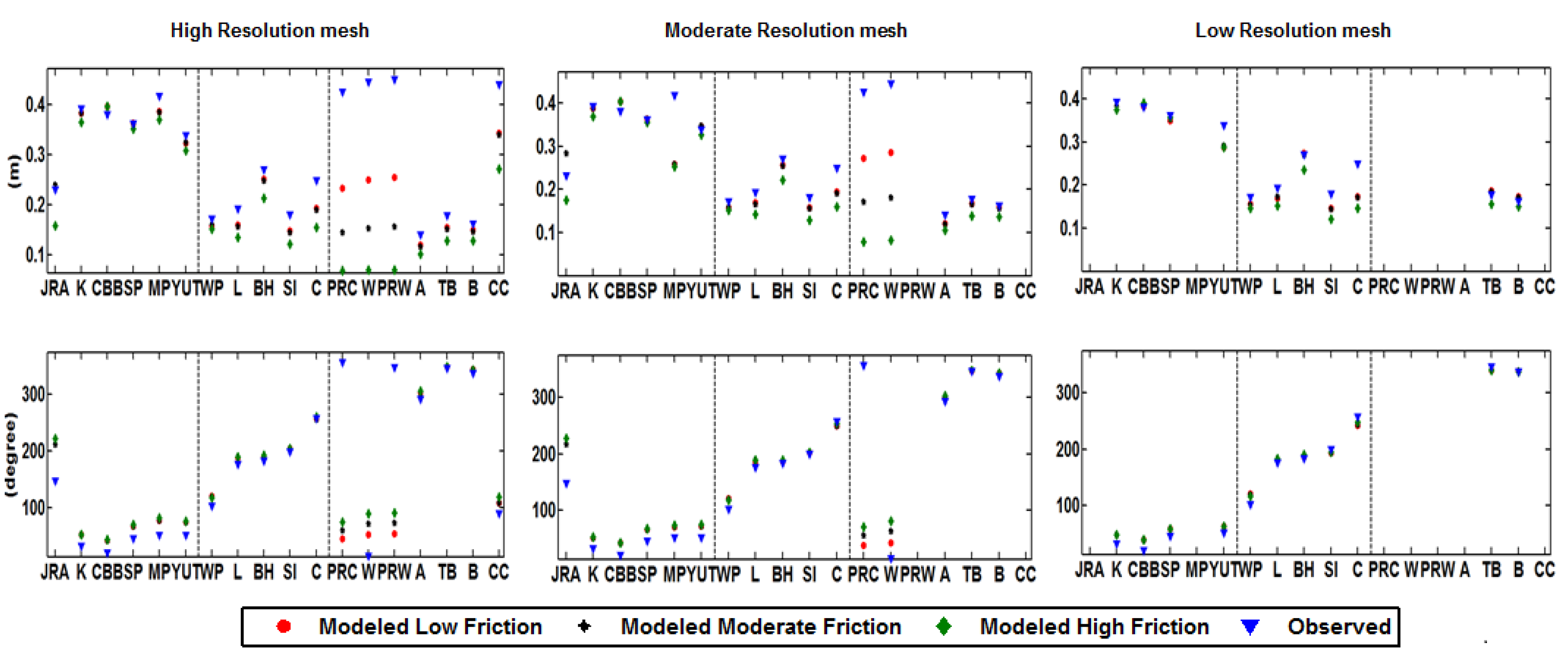
The sensitivity of the amplitude of the major constituent (M₂) is analyzed by quantifying range of the modeled M₂ amplitudes, i.e., the modeled amplitude by using a low Manning’s n coefficient minus modeled amplitude by using a high Manning’s n coefficient. Figure 6 displays the amplitude and phase of the M₂ simulated by using each level of roughness (low, moderate, and high). Furthermore,

Table 6. Average Range of modeled M₂ amplitudes (m).

Numerical Mesh	Lower Bay		Middle Bay		Upper Bay
	Region “a”	Region “b”	Region “a”	Region “b”	Region “a”	Region “b”
High Res. Mesh	0.12	0.01	-	0.03	0.18	0.03
Mod. Res. Mesh	0.16	0.01	-	0.03	0.20	0.02
Low Res. Mesh	-	0.00	-	0.02	-	0.03

summarizes the information provided by Figure 6 for this constituent. At the lower bay, the analysis of the simulations performed on the three meshes showed that the range was around 0.00–0.01 m for all stations, except JRA station that lies on the region “a”, and it varied between 0.12 and 0.16 m. At the middle bay, all meshes performed similarity, showing a minimum degree of sensitivity in all stations for this tidal constituent. BH was the station presenting the largest sensitivity; the range of the modeled amplitudes was 0.04 m. At the upper bay, the range of those stations located in the region “b” varied between 0.02 and 0.03 m for the simulations performed on the three numerical meshes. Conversely, the modeled amplitudes were more sensitive in the region “a”, i.e., a larger range was found for PRC, W, and PRW stations. Here the differences between M₂ modeled amplitudes by using high and low friction varied up to 0.20 m. Table 6 also shows that there is no effect of resolution on the sensitivity of the M₂ amplitude to Manning’s n coefficient since three numerical meshes provided similar ranges in each region.

Authors such as Kerr et al. (2013) [41] have studied the tide amplitude sensitivity to bottom friction formulation (with and without a lower limit on the bottom drag coefficient). They observed that both formulations performed relatively similar, concluding that tidal model is not sensitive to these formulations. Additionally, the control stations were divided into three regions: open, protected and inland. The MAEs obtained from the simulations using the limit and without lower limit formulations are fairly similar in each region. Passeri et al. (2011) [28] studied the astronomical tide response to bottom roughness by the assigning three different levels of roughness in rivers, bays, and marshes in a study case in Florida. They found differences in the modeled M₂ and K₁ amplitudes ranging between 0.00 and 0.04 m by using a high and low friction. However, those values were found in rivers and bays areas indistinctly, i.e., both areas exhibited the same sensitivity. The values found here are consisted with those values reported by Passari et al. (2011) [28] although none of these previous works observed different sensitivity in rivers and bays. The reason of this larger sensitivity in rivers could be explained by the fact that region “a” (river) is shallower (between 1 and 12 m) in comparison with the rest of the bay, region “b”, which reaches up to 30 m. According the Equation (1), the bottom stress is inversely related to the water depth, being more significant in shallow areas. Thus, Manning’s n coefficient is more relevant in shallow areas; bottom stress and water elevation is more sensitivity to this coefficient in the region “a” than region “b”. Previous authors did not provide any information about the morphology or bathymetry of their study areas, therefore authors´ hypothesis cannot be confirmed with their works.

Figure 6 and

Table 7. Mean absolute error (MAE) of the M₂ amplitude (m).

Numerical Mesh	Friction	Lower Bay		Middle Bay		Upper Bay
		Region “a”	Region “b”	Region “a”	Region “b”	Region “a”	Region “b”
High Resolution Mesh	High	0.07	0.02	-	0.06	0.37	0.04
	Mod	0.01	0.01	-	0.03	0.29	0.02
	Low	0.04	0.01	-	0.03	0.19	0.02
Moderate Resolution Mesh	High	0.06	0.02	-	0.05	0.35	0.03
	Mod	0.05	0.01	-	0.03	0.26	0.01
	Low	0.10	0.01	-	0.03	0.16	0.01
Low Resolution Mesh	High	-	0.02	-	0.05	-	0.02
	Mod	-	0.02	-	0.03	-	0.01
	Low	-	0.02	-	0.03	-	0.01

were used to analyze the model performance by comparing against observed data. The results provided by the three meshes present a noteworthy similarity; overall, the simulations underestimated the amplitude of the M₂ tidal constituents. Note that the results from MP, PRW, A, and CC stations were excluded of the calculation of the MAE, Table 7. In the region “b” of the lower bay, this metric showed that all friction simulations performed relatively similar, counting errors between 0.01 and 0.02 m. However, in the region “a”, the moderate friction simulation provided the lower MAE, 0.01 m, against 0.07 m or 0.04 m obtained for high and low friction respectively (high resolution mesh). The MAE of the middle bay stations showed that all frictions performed correctly (the maximum MAE was 0.06 m), but the moderate and low friction simulations produced a slightly lower error (0.03 m). Similarly as the lower bay, an increase of resolution did not lead to a lower error. In the region “b” of the upper bay, according to the MAE, the low and moderate frictions simulations performed similar with a minimum error (MAE equal to 0.01 m). However, Figure 6 clearly displayed that the model did not properly simulate the propagation of the tidal wave throughout one of the CB tributaries, region “a”. This is undoubtedly seen on PRC, W, and PRW stations, where the model highly under predicted the observed data. This region produced the largest errors, and the lower MAE, 0.19 m and 0.16 m, was produced by the low friction simulations.

Previous works using the ADCIRC model to simulate astronomical tide in CB [42] also observed that the model consistently underestimated the recorded data. This analysis was carried out for three stations located throughout the bay: CBB, BH, and TB. Shen et al. (2006) [4] simulated water levels by using the Unstructured, Tidal, Residual Intertidal, and Mudflat model (UnTRIM), and carried out a tidal harmonic analysis. This model, in general, slightly overestimated the observed data, and M₂ amplitude was more accurate predicted in the lower than the upper bay. Unfortunately, these studies excluded some stations such as JRA, PRC, W, or PRW where ADCIRC provided less accurate results. This study demonstrated that large tributaries may need to use different Manning’s n values. For instance, Manning’s n coefficient of 0.035 along James River performed properly, but a value of 0.02 overestimated the M₂ amplitude. Potomac River exhibited a different pattern, and a value of 0.02 widely underestimated this amplitude. Conversely, Manning’s n coefficients of 0.02 or 0.012 were seen to perform similarly and to reduce the error in region “b”. Another significant point is that three meshes displayed same errors, indicating that (1) this level of resolution did have not impact on the results, and (2) the M₂ amplitude was not sensitive to the location of the open boundary.

Figure 6 depicting the modeled and observed phases and

Table 8. Average range of modeled M₂ phase (degree).

Numerical Mesh	Lower Bay		Middle Bay		Upper Bay
	Region “a”	Region “b”	Region “a”	Region “b”	Region “a”	Region “b”
High Res. Mesh	12	2	-	2	34	3
Mod. Res. Mesh	14	2	-	2	32	1
Low Res. Mesh	-	0	-	3	-	1

displaying the range of the modeled M₂ phase, showed that the phase was not sensitive to Manning’s n coefficient in region “b”, independently of the level of resolution or portion of the bay. However, similarly to the modeled amplitude in the region “a”, the phase was more sensitive to Manning’s n coefficient at JRA, PRC, W, and PRW stations. The modeled phase varied around 12–14 degrees in the lower bay, and 30–40 degrees at the upper bay. As Kerr et al. (2013) [41] work argues, we found that the harmonic analysis displayed that the astronomical tide phase is less sensitive to mesh resolution and roughness.

Similarly to the amplitude, the accuracy of the modeled phase is significantly fair for those stations located in the region “b”, and a greater phase lag is observed at the stations located at the region “a”, Figure 6 and

Table 9. Mean absolute error (MAE) of the M₂ phase (degree).

Numerical Mesh	Friction	Lower Bay		Middle Bay		Upper Bay
		Region “a”	Region “b”	Region “a”	Region “b”	Region “a”	Region “b”
High Resolution Mesh	High	75	21	-	9	76	5
	Mod	65	21	-	8	61	5
	Low	63	21	-	8	44	5
Moderate Resolution Mesh	High	80	21	-	8	71	4
	Mod	69	20	-	9	54	4
	Low	66	20	-	9	35	4
Low Resolution Mesh	High	-	14	-	8	-	3
	Mod	-	14	-	9	-	3
	Low	-	15	-	9	-	3

. Thus, at the lower bay, low friction simulations showed the lower gap (63–66 degrees). The model did not either appropriately capture the phase of the M₂ tidal constituents at PRC, W, and PRC stations (upper bay). These stations located on region “a” exhibited a phase lag up to 44° by using a low friction value. The low friction simulations provided better performances in the region “a” in the lower and upper bay.

A noteworthy point is that there was an improvement in the tidal phase lag of this semidiurnal tidal component as the tidal wave propagates throughout the CB for all simulations. For instance, the MAE for high resolution mesh showed that M₂ phase lag at the lower bay is 21 degrees, against the 8 degrees at the middle bay and 5 degrees at the upper bay (region “a”). It is not clear why the model reduced the error simulating tidal phase in the upper bay, and therefore future analysis should be carried out to explore this phenomenon. Another remarkable fact is that the low resolution mesh produced the lower MAE than high resolution mesh.

3.1.2. Storm Surge in Waterways

The sensitivity of the peak of the storm surge is analyzed by quantifying the peak of the storm surge simulated by using a low Manning’s n coefficient minus the peak simulated by using a high Manning’s n coefficient (range),

Table 10. Average range of the modeled peak during Hurricane Irene and Sandy in meter.

Hurricane Irene
Numerical Mesh	Lower Bay		Middle Bay		Upper Bay
	Region “a”	Region “b”	Region “a”	Region “b”	Region “a”	Region “b”
High Res. Mesh	0.29	0.11	-	0.11	0.35	0.10
Mod. Res. Mesh	0.29	0.05	-	0.06	0.33	0.08
Hurricane Sandy
Numerical Mesh	Lower Bay		Middle Bay		Upper Bay
	Region “a”	Region “b”	Region “a”	Region “b”	Region “a”	Region “b”
High Res. Mesh	0.56	0.04	-	0.05	0.43	0.04
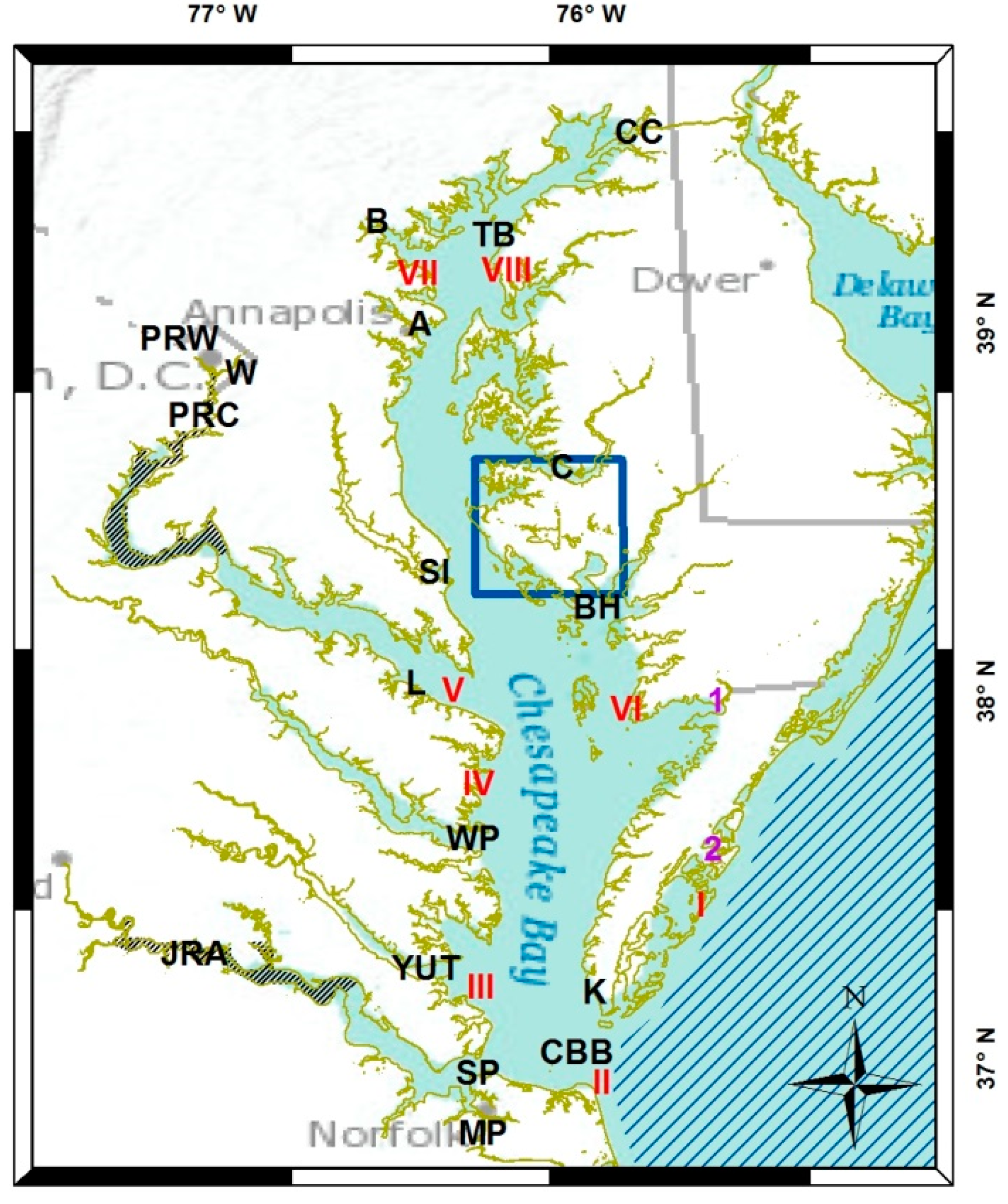
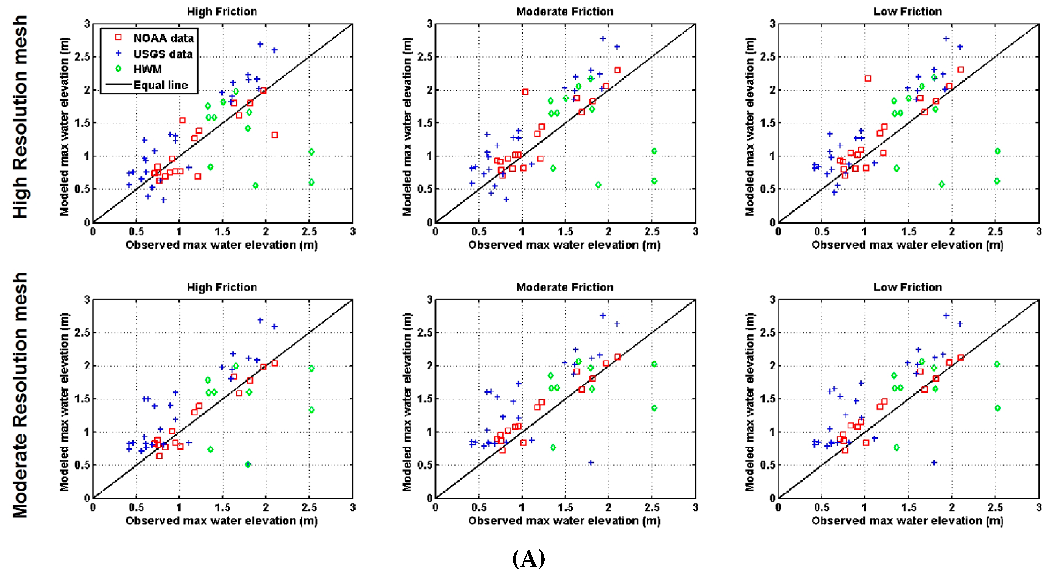
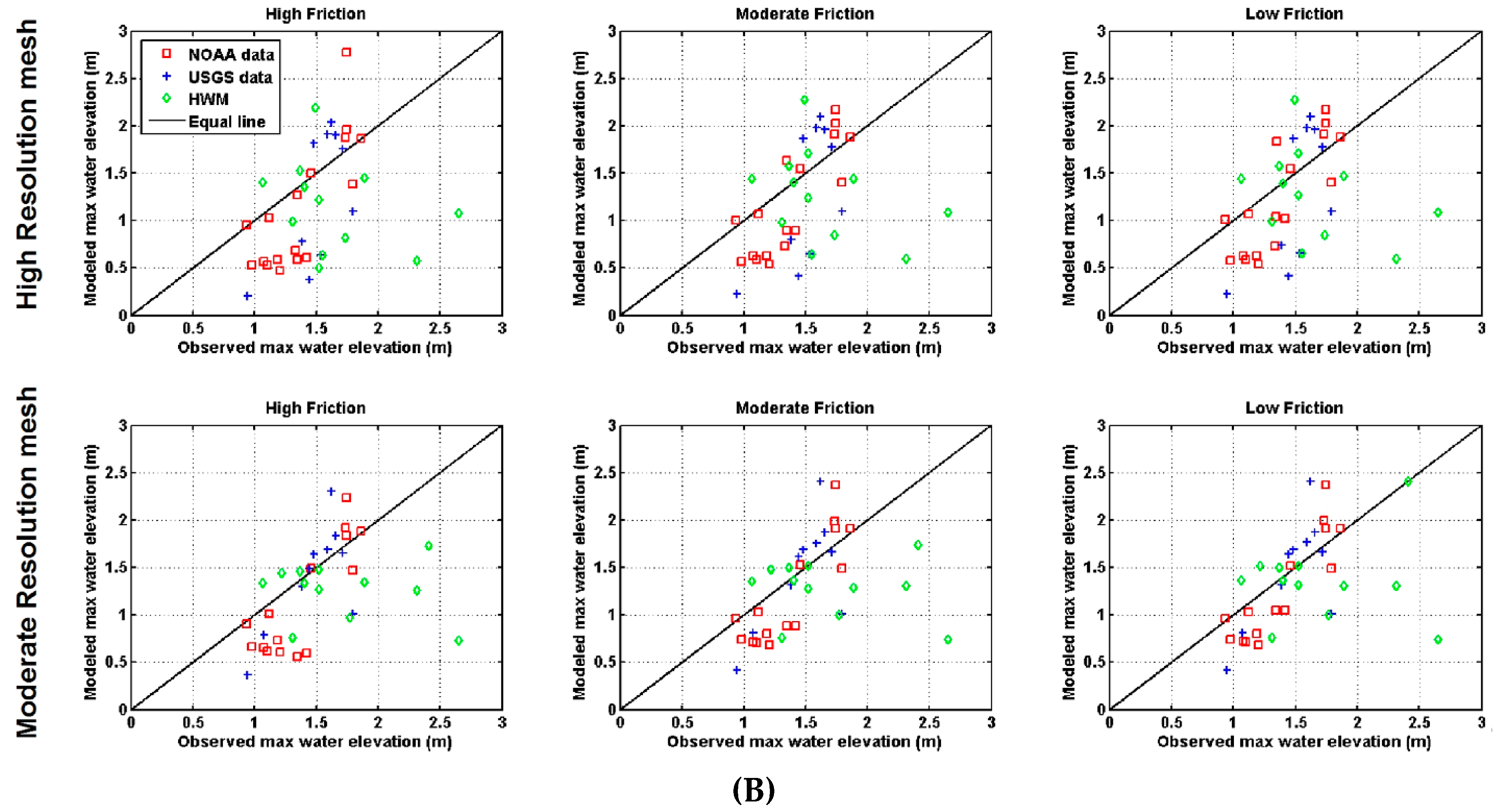
Mod. Res. Mesh	-	0.05	-	0.06	0.47	0.07

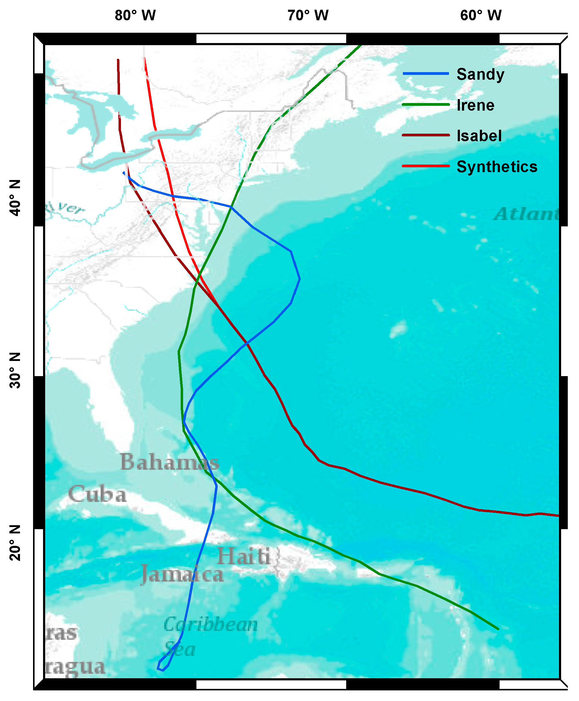
. Besides NOAA stations, US Geological Survey rapid deployment data and High Water Marks (HWM) were included in this study, and they were also categorized as lower, middle and upper bay. In order to preserve the reliability of the results, a validation of the model performance against observed data is shown in Figure 7. Note that Hurricane Irene and Sandy were validated by using high and moderate resolution meshes and the three levels of roughness.

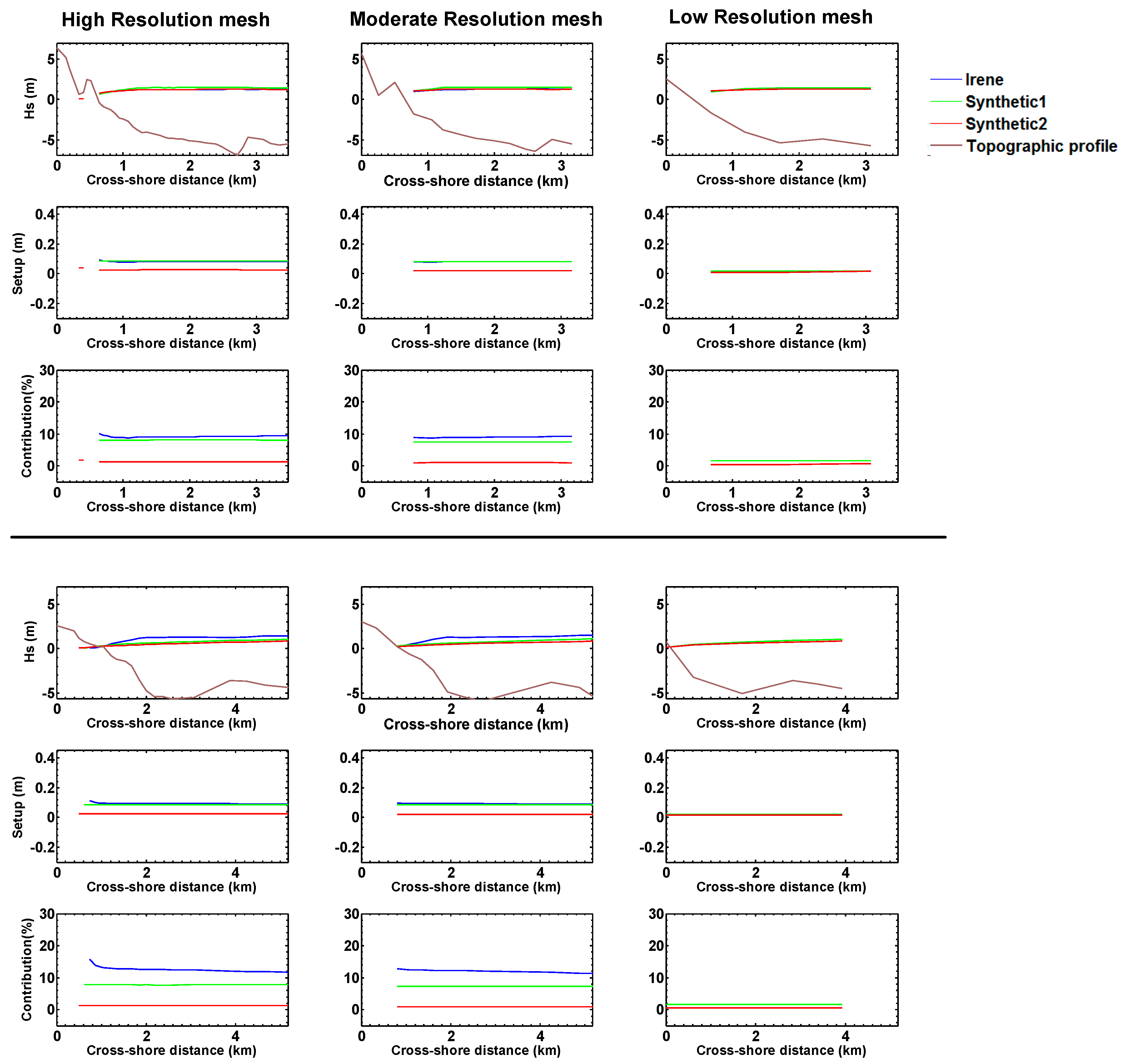
Hurricane Irene hindcast in the lower bay exhibited a range between 0.05 and 0.11 m in the region “b”. Meanwhile, the range in the region “a” increased up to 0.29 m. Note that this range was larger than the range observed in amplitude of M₂ sensitivity analysis (0.12–0.16 m). In the region “b”, the model performed similarly in the middle bay as the lower bay; the range was around 0.11 and 0.06 m. In the upper bay, the range counted for 0.10 and 0.08 m in the region “b”, and 0.33–0.35 m in the region “a”. The range in this region was also larger than the M₂ amplitude (0.18–0.20 m).

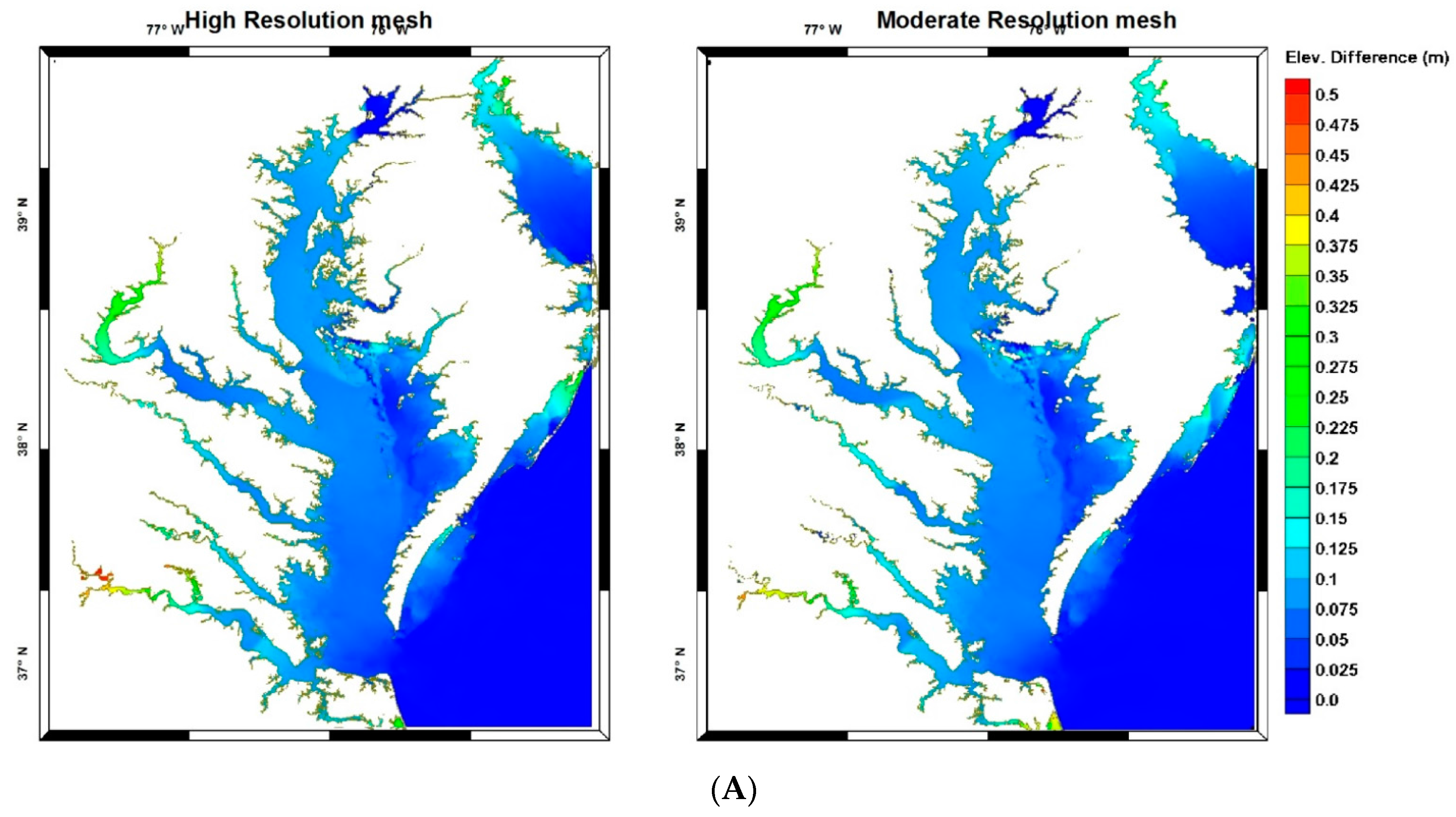
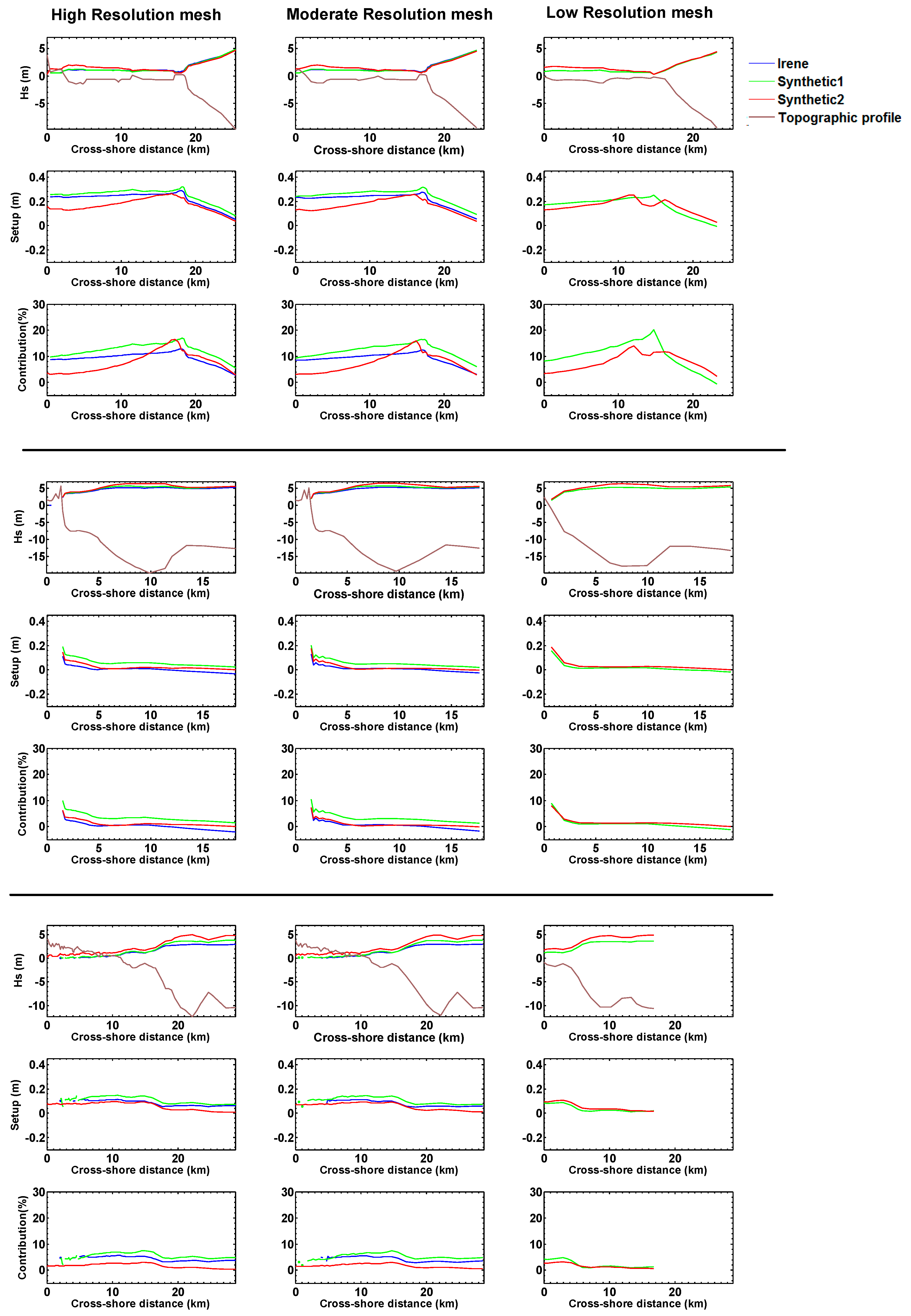
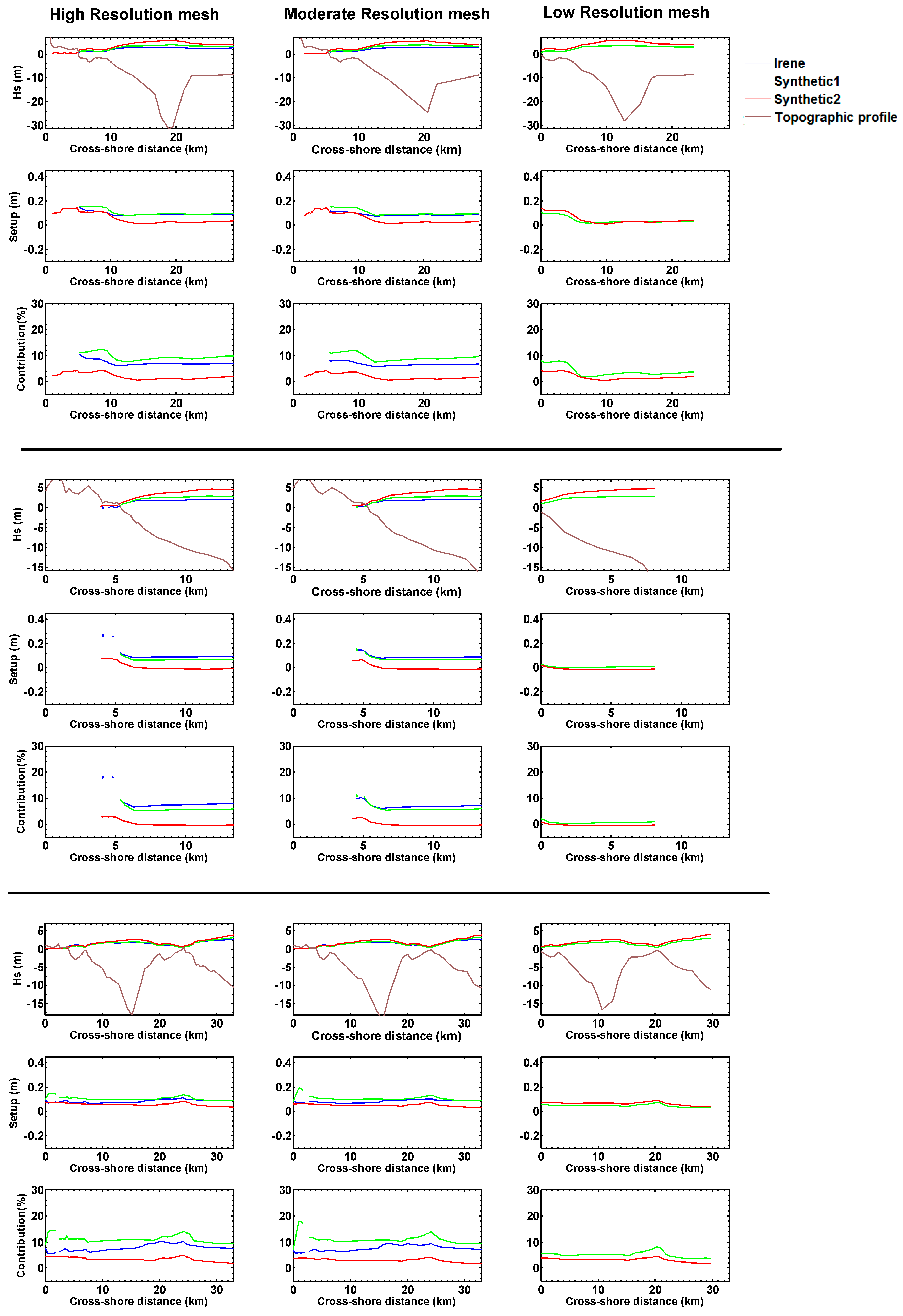
Ranges along the entire CB for Hurricane Irene are shown in Figure 8A. Left plot depicts high resolution mesh and right plot moderate resolution mesh. The high friction case reduced maximum water levels up to 0.15 m in the region “b” for both meshes. The differences were minimal in the lower bay, where the higher storm tide levels were observed. Further, as we discussed earlier, the difference in the upper bay showed the same magnitude. However, those ranges increased in the region “a” up to 0.5 m in James River and around 0.40 m in Potomac River. As it was shown in the Table 10 for certain specific locations, during Hurricane Irene, the level of resolution did have no impact on the storm surge sensitivity.

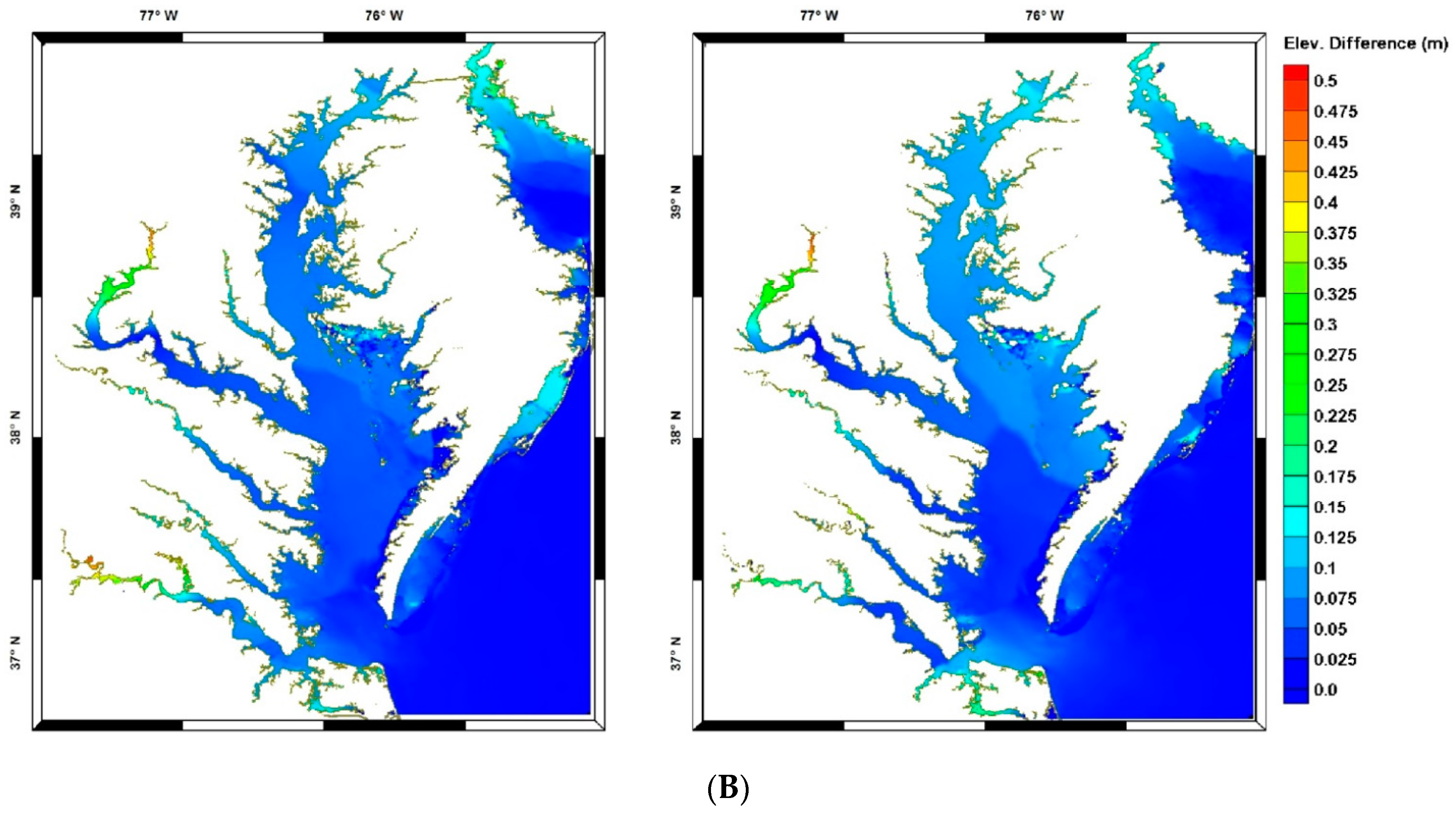
Hurricane Sandy hindcast displayed a larger range than Hurricane Irene in the regions “a”, (Figure 8B). Therefore, this range increased up to 0.56 m in the lower bay and 0.43–0.47 m in the upper bay. The performance of the model in the regions “b” was similar and the peaks ranged between 0.04 and 0.07 m.

Along the entire CB, the high friction scenario reduced maximum water levels in region “b” less than 0.10 m (Figure 8B). Meanwhile, the peak decreased around 0.40–0.60 m along the James River and Potomac River. These results also displayed that rivers exhibited a larger sensitivity to bottom friction than bay and shore adjacent areas. Likewise as Hurricane Irene, no differences were observed between both panels, as it is shown in (B), and therefore, the model displayed the same level of sensitivity of maximum water levels to Manning’s n coefficient for these two degrees of mesh resolution.

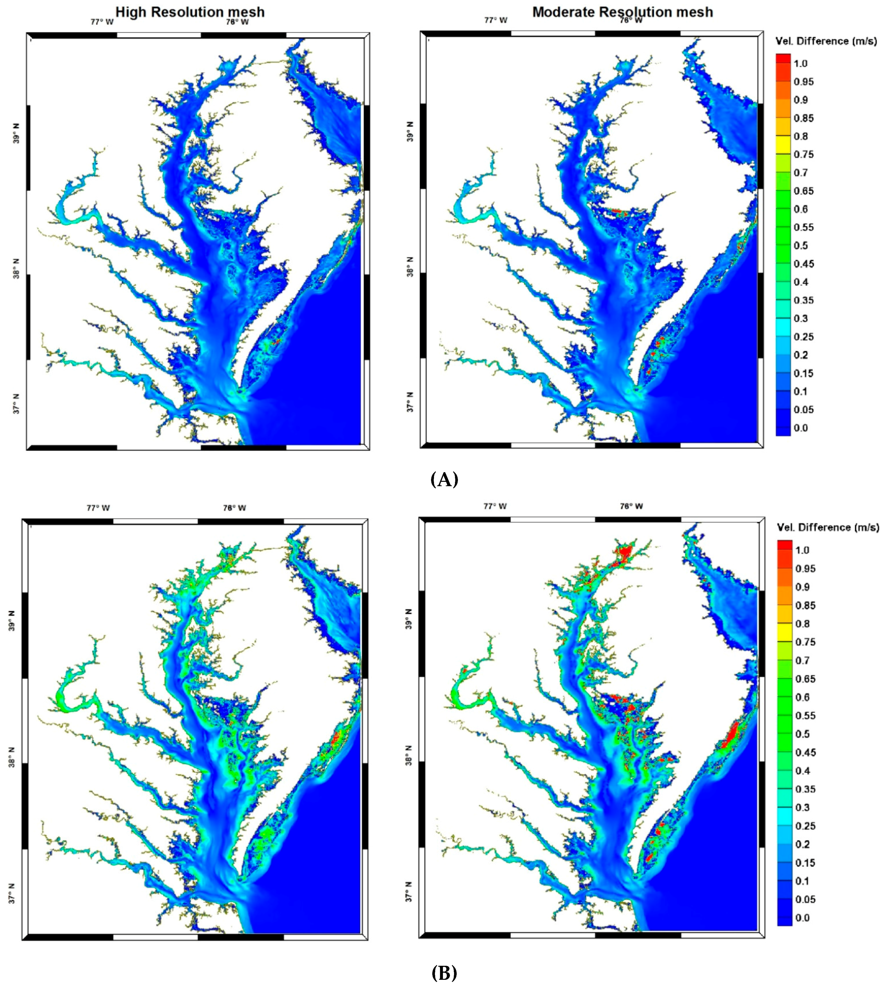
Figure 9A shows the differences between the maximum velocities (low and high friction scenario) simulated on the high and moderate resolution mesh for Hurricane Irene. Overall, both meshes performed moderately similar; the model showed the same level of sensitivity to maximum currents by using different resolutions. Currents were reduced by 0.20–0.30 m/s in the shallower areas of the bay (region “a” and “b”); meanwhile the currents did not decrease along the main axis of the bay. Currents behind the barriers of Delmarva Peninsula were reduced up to 0.80 m/s. No significant current reduction was found at James River and Potomac River.

On the other hand, during Hurricane Sandy high friction attenuated maximum currents up to 0.80–1.00 m/s at the upper bay and marsh areas (high resolution mesh) as it is shown in Figure 9B. This attenuation extended throughout wider areas on the simulations performed on the moderate resolution mesh, indicating that the results produced by this mesh were more sensitive than high resolution mesh. Currents in Potomac River also were attenuated by 0.50–0.70 m/s, meanwhile in James River the high friction reduced currents by up to 0.40 m/s.

In the same study referred previously, Kerr et al. (2013) [41] also studied the sensitivity of the storm tide driven by Hurricane Ike to Manning’s n bottom friction formulation. They reported that a lower limit on the bottom drag coefficient reduced water levels up to 0.75 m in waterways areas respect to the standard quadratic formulation with no limit, which is used in this work as well. Additionally, they estimated that the largest reduction in currents, around 1.00–1.75 m/s, by using the lower limit formulation occurred along the storm track, and away from the storm track this reduction ranged between 0.25 m/s and 1.00 m/s. These reductions in water levels and currents are larger than those that we found in this study. However, it is important to underline that Hurricane Ike was significantly stronger than the storms analyzed here. For example, during Hurricane Ike the maximum water levels and currents simulated reached peaks of 5.00 m and 5.00 m/s. They were considerably larger than the values reached during Hurricane Irene and Sandy in the CB (2.00 m and 1.50–2.00 m/s).

The sensitivity analysis performed by Passeri et al. (2011) [28] by using Hurricane Denis showed the differences between using a high and low friction scenario ranged from 0.00 m to 0.21 m for 203 stations located in inland and waterway area. The maximum water levels observed during this storm were around 1.80–2.70 m, similar values as we observed in this work. Also, they observed the smallest differences occurred along the coastline. These findings are in concordance with the results obtained here, although stations located in rivers showed a larger sensitivity. The fact that the range of Manning’s n assignments in region “a” was wider than region “b” did not explain this higher sensitivity only in riverine areas, and it also could be explained by the lower depth in river regions.

3.1.3. Storm Surge in Overland Areas

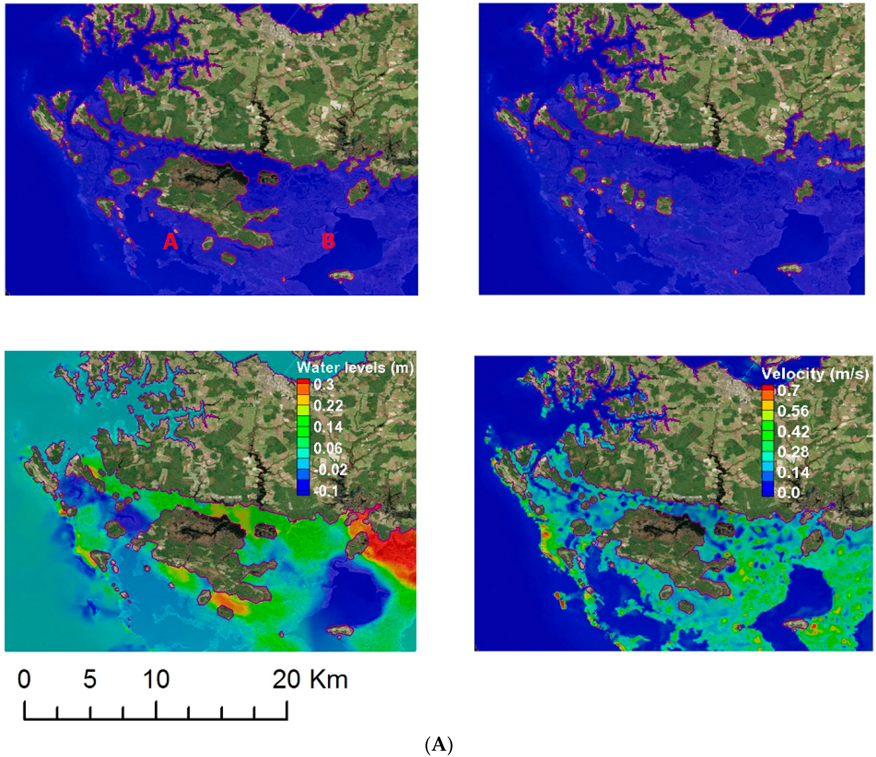
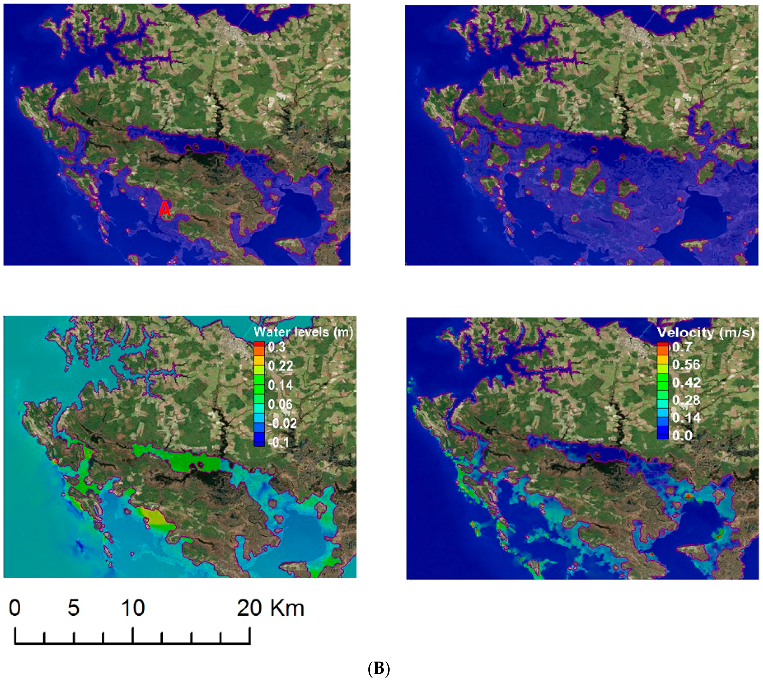
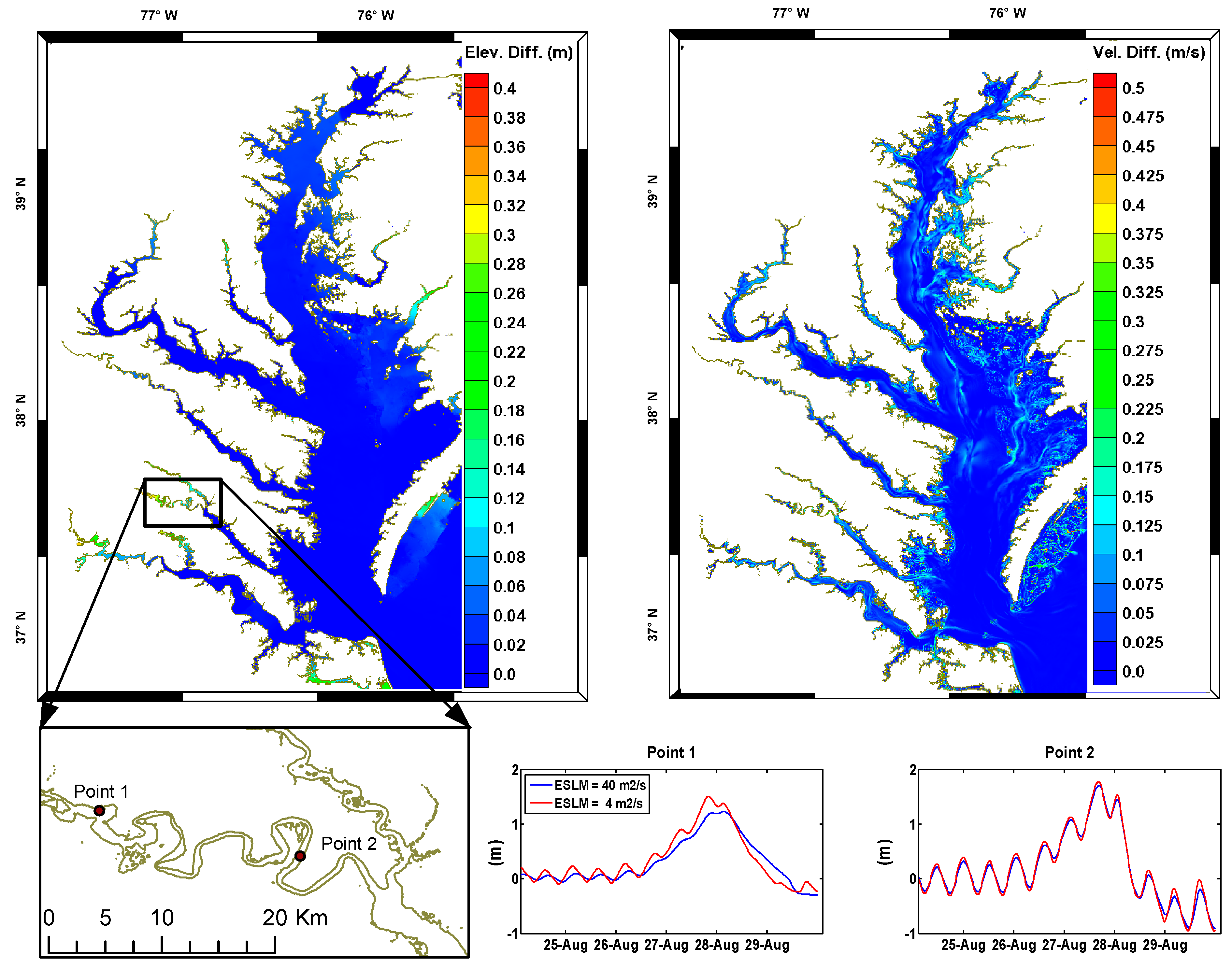
The effect of bottom friction on flood extension, maximum water levels and currents is explored on Figure 10 for Hurricane Irene (A) and Sandy Hindcast (B). It is observed that the low bottom friction simulation produced a larger inundation area during Hurricane Irene; the flooding area increased more than 1100 ha, especially in the central part of the study area, which was not inundated by the high friction scenario. The effect of bottom friction on the peak of the storm, (maximum elevation produced by the low minus high friction runs), was spatially variable, since it is highly dependent on local features and topography [9], and the largest difference was up 0.30 m. The high friction produced also higher water levels at some wet areas adjacent to the shoreline or channels. A higher friction on inland areas produced that the flood wave did not widely inundate inland areas and the water piled up over the shoreline. The currents were reduced by up to 0.70 m/s for the high friction scenario and no changes were observed in open water areas.

The flood extension also exhibited to be sensitive to Manning’s n coefficients for Hurricane Sandy. Flooded zones produced by the high friction run were limited to adjacent areas to the shoreline and channels, as it is shown in Figure 10B; high friction reduced 1500 Ha the flood extension. The largest reduction of the peak of the storm tide produced by the high friction simulation was 0.20 m, and no appreciable accumulation of water is observed in the shoreline as the previous case. Moreover, the high friction simulation led to a maximum reduction of currents around 0.50–0.70 m/s.

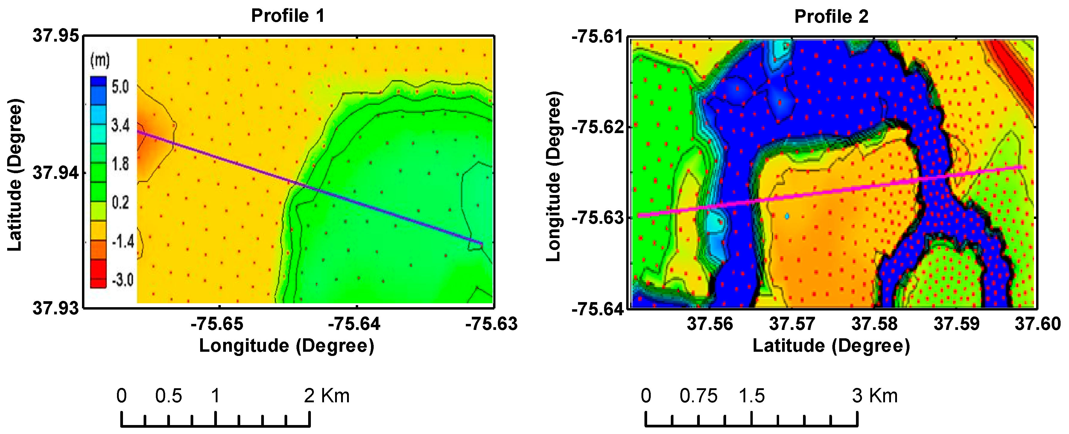
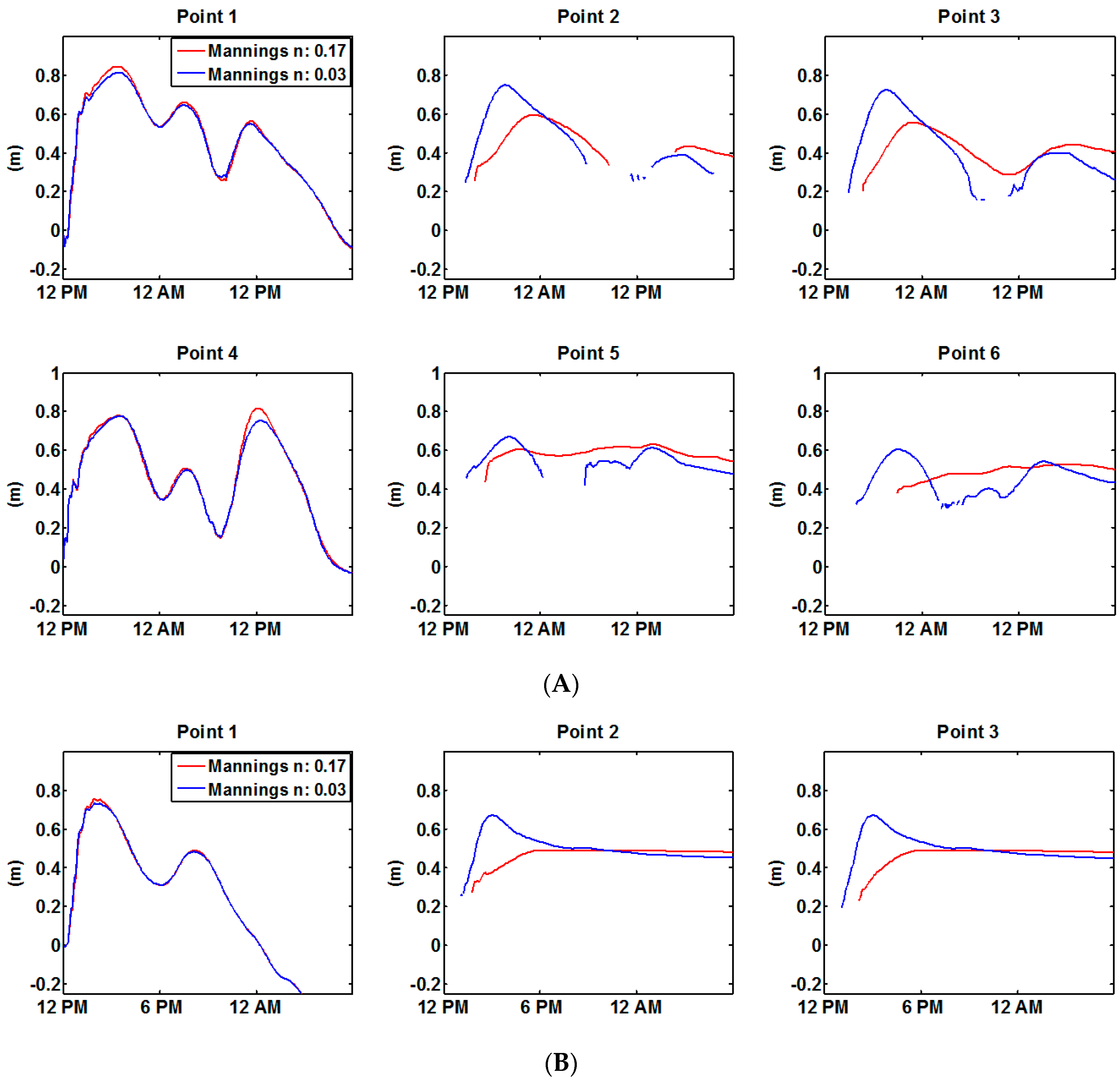
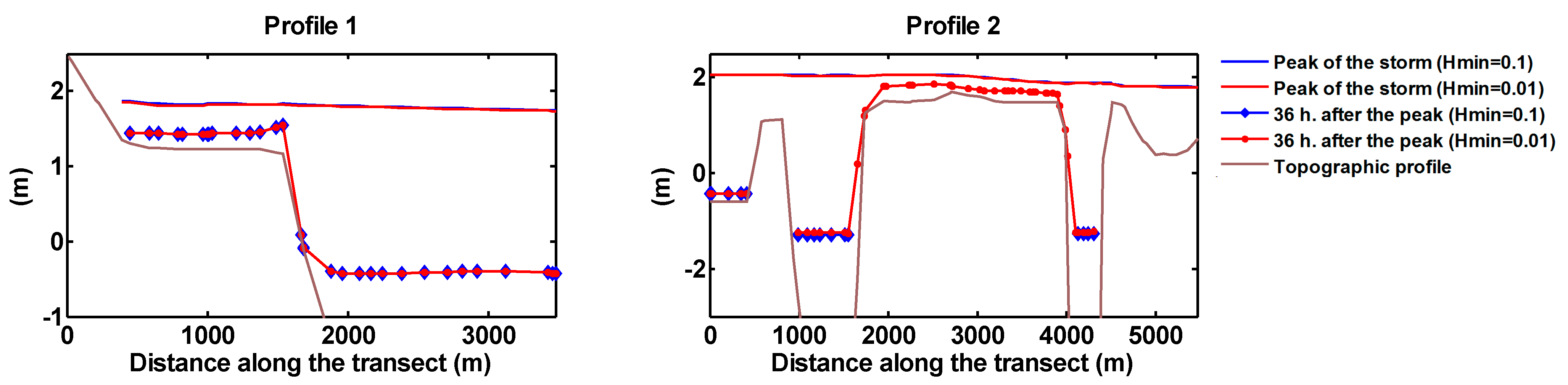
Figure 11A shows water levels time series during Hurricane Irene at three stations along Transect A and B displayed in Figure 10. Points 1 and 4 are found in open water, Points 2 and 5 closely to the shoreline, and Points 3 and 6 are located further inland. These points were spaced between 100 m and 200 m along the each transect. Water levels simulated by the low and high Manning’s n coefficients runs at Points 1 and 4 exhibited slight differences, but it is noteworthy to point out that they were at wet locations. As it was seen in Figure 10A, a higher friction on inland areas increased water levels in wet areas by the shoreline. Point 2 and 3 showed the model is highly sensitive to Manning’s n coefficient. A lower friction resulted in a higher peak of the water levels (0.15 m) and, also this peak was reached about 4–5 h earlier. Point 3 presented a similar behavior, but additionally a higher friction obstructed the receding of the flood wave increasing the flood depth during the low tide.

A higher bottom friction at Point 5 and 6 led to a slower advancing and receding movement of the flood wave; it produced a lower peak and longer flooding duration. The storm surge attenuation observed between Point 2 and 3, and between Point 5 and 6 in the high friction scenario was similar as the storm surge attenuation observed in the low friction scenario.

Figure 11B displays two different time series water levels during Hurricane Sandy. It is readily observed that the flood wave was very sensitive to Manning’s n coefficients in Point 2 and 3. The low friction run showed a noticeable peak and a gradual receding of the flooding. The high friction simulation, instead, significantly dampened the peak and retarded around 8 h this peak respect to the low friction run. Once the water level reached its maximum, the surface level maintained constant (high friction simulation). Finally, note that the points of Transect B are not analyzed because the simulated flood wave by using high friction did not propagate as far as the previous storm tide, and Point 5 and 6 were not inundated.

Passeri et al. (2011) [28] also affirmed that water levels are more sensitive to Manning’s n coefficient in inland areas. Hurricane Irene and Sandy flood wave characteristics (flood extension, wave propagation, maximum water levels, and maximum currents) in inland areas showed to be clearly sensitivity to bottom friction. Manning’s n coefficient of 0.03 and 0.17 might be associated with pasture or grassland and mixed forest [31], therefore, the model is very sensitive to the land cover classification. It might confirm what Ferreira et al. (2014) [43] demonstrated, and an incorrect land cover choice may lead to error in surge of 7.0%. Resio and Westerink (2008) [9] discussed that an increased frictional resistance slows the rate the flood wave moves inland. It could increase water levels in portions of the system, and attenuates the surge amplitude. These processes were observed on Figure 11A.

Previous studies and the present work suggest that the election of Manning’s n coefficient between 0.012 and 0.03 in waterway areas might not have a significant impact on the storm surge propagation in the CB. Conversely, a correct selection in some tributaries is vital to properly simulate storm surge. As Kerr et al. (2013) [41] suggested, an adequate simulation of tidal physics is important in storm surge model because they contribute to water levels and currents during hurricanes. Therefore, this study supports the idea to use a moderate value of Manning’s n coefficient in James River and a low value in Potomac River. Additionally, these findings demonstrated that a correct selection of the Manning’s n coefficient in overland is essential for model accuracy.

3.2. Interaction of Wind Waves and Circulation

Water levels driven by Hurricane Irene, Synthetic storm 1, and Synthetic storm 2 were simulated by using ADCIRC and the couple version (ADCIRC + SWAN) to study the wave radiation stress gradients contribution to overall water levels. Further, these simulations were performed on the three numerical meshes. H_s during the peak of the storm, wave setup, and relative contribution (i.e., the contribution of wave setup to overall water levels in terms or percentage) along eight profiles shown previously in Figure 5 were analyzed.

Profile I shown in Figure 12 showed a gradual reduction in the significant wave height as the waves propagated to the shoreline for the three events. The breaking point, i.e., the location where a reduction of H_s was observed on the Figure 12, Figure 13 and Figure 14, was located offshore of 25 km for all simulations. Additionally, the wave setup was observed to vary roughly linearly to the variation of the depth along this profile (from 25 km to 18 km). Two different slopes are found in the high and moderate resolution meshes, and only one in the low resolution mesh, since this mesh did not capture properly some topographical features such as the barrier island. Both maximum wave setup and relative contribution simulated on high and moderate resolution mesh displayed similar values; wave setup ranged between 25 cm and 32 cm and relative contribution varied between 12% and 16% for these three storms. The low resolution mesh led to a lower wave setup observed during Synthetic storm 1 and Hurricane Irene. However, this mesh produced the maximum relative contribution of wave setup to water levels, around 20%, for the Synthetic storm 1, since this mesh simulated the lowest peak of the storm in this profile. After the barrier island, waves propagated over a deeper area and increased H_s; therefore, a progressive reduction of wave setup was observed.

Profile II shown in the Figure 12 crosses the main channel of the bay, where the waves increased their height. The wave breaking line for all storms simulated on the three meshes was observed around the 5–7 km (cross-shore distance), and wave contribution to water levels begun to have a larger effect. The variation of wave setup along Profile II behaved approximately linear with respect to the variation of the depth with a steeper section close to the shoreline. This was more notorious for the high and moderate resolution mesh. The three meshes provided similar wave setup (10–20 cm) and relative contribution (6%–10%) values. Profile III is located inside the bay and the H_s observed were clearly lower, Figure 12. Beyond the channel, between 21 km and 18 km (high and moderate resolution mesh) and 10 km (low resolution mesh), waves started to break over the beach slope, and the wave setup was more significant reaching at the shoreline round 8–15 cm, with higher values in the two first meshes. Note that the low resolution mesh does not widely cover inland areas, and the first point of this profile has an elevation of 1 meter below the water. It could imply that waves did not totally break over the profile, and therefore, a lower maximum wave setup in this mesh was observed. The relative contribution at the shoreline accounted for around 3%–8% in the high and moderate resolution mesh and 3%–5% in the low resolution mesh.

Profile IV, V, and VI, situated on the middle bay, are shown in Figure 13. Profile IV exhibits a similar profile as Profile III. Synthetic storm 2 drove the highest waves, and its breaking line was found around the 15 km (high and moderate resolution) and 10 km (low resolution mesh). Hurricane Irene and Synthetic 1 storm drove less energetic wind waves, and they broke closer to the shoreline. Therefore, the wave setup for each event increased from these points. The high and moderate resolution mesh provided similar wave setup and relative contribution values, meanwhile the low resolution mesh produced lower values. For example, the estimated wave setup and relative contribution by using those meshes during Synthetic storm 1 was 15 cm and 12%, and by using the low resolution mesh was 10 cm and 8%.

Profile V is situated further from the mouth of the bay (Figure 5) and H_s decreased respect to the previous profile for all the storms. The effect of wave radiation stress gradients on water levels was less significant in this profile for these storms around 8–12 cm (high and moderate resolution), and especially in the low resolution simulations. This profile, similarly as Profile III, does not completely emerge, and it led to a lower maximum wave setup. Profile VI crosses through an island before reaching the main channel and the shoreline. The maximum wave setup was found at this island, where the wave significantly reduced most of their energy, and then, it maintained almost constant. The relative contribution to overall water levels in the shoreline ranged between 4% and 12%, high and moderate resolution mesh; as same as the previous profiles, low resolution mesh simulation produced lower values, 4%–6%.

Profile VII and VIII are located at the upper bay, where the waves arrived after traveling through the entire bay, reducing significantly their H_s (Figure 14). Wave setup along profile VII maintained significantly constant with values between 2 cm and 8 cm for the high and moderate resolution and 2 cm for the low resolution mesh. The relative contribution of wave setup simulated by using those meshes was up to 10%. Profile VIII behaved likewise as Profile VII, although it is important to point out that the relative contribution of wave setup, even at the upper bay, was up to 15% for Hurricane Irene.

Table 11. Wave setup and relative contribution to water levels driven by the Synthetic 1 storm.

Profile	High Resolution Mesh		Moderate Resolution Mesh		Low Resolution Mesh
	Setup (m)	Contribution (%)	Setup (m)	Contribution (%)	Setup (m)	Contribution (%)
1	0.32	17	0.31	16	0.25	20
2	0.19	10	0.20	10	0.16	9
3	0.15	7	0.14	7	0.09	5
4	0.15	12	0.16	12	0.10	8
5	0.12	10	0.13	10	0.02	2
6	0.15	15	0.19	18	0.05	5
7	0.08	8	0.08	7	0.02	2
8	0.08	8	0.08	7	0.02	2

briefly summarizes the results obtained by the Synthetic storm 1 simulation.

Harris (1964) [44] established that the peak of water elevations reported from the shores of an estuary should be less than for those reported from the open coast because the peak of wave heights in the estuary are generally less than those on the open coast. This is consistent with the work of several authors that have demonstrated that the offshore wave height is the primary control on wave setup since it provides the energy available for the production of setup [32,45,46]. This phenomenon was also observed on this work, and the wave setup was lower in the upper bay where the wave energy was reduced due to the shallow depth and limited fetch. Some of the profiles, e.g., Profile 1 clearly showed that wave setup slope inside the surf zone is proportional to the beach slope as expressed by Longuet-Higging and Stewart (1964) [32] and Guza (1981) [46]. Additionally, the effect of the barrier island in this profile was very substantial on the wave setup since its steeper slope inside the breaking area led to a significant increment of wave setup [9]. Stephen et al. (2011) [46] demonstrated that wave setup is also highly influenced by the profile shape. Thus, the wave setup could differ substantially as the result of the variability of the cross-shore profile shape. It could be seen on Profile 1 and 2, both located mainly outside the bay, but the simulated wave setup moderately varied between those two profiles. Further, the smoothed profile from the low resolution mesh significantly reduced the wave setup. Another factor affecting the wave setup is the angle of wave propagation and breaking. The wave radiation stress gradients from waves breaking at an oblique angle to the coast are balanced by a steady force that generates the wave setup, but also a longshore current. The generation of this current parallel to the coast leads to a lower wave setup scenario than those waves breaking parallel to the coast [33,44]. Sheng et al. (2010) [1] observed in their study in the CB and Outer Banks during Hurricane Isabel that comparable wave heights in CB and North Carolina drove different wave-induced water elevation. Thus, in North Carolina, the wind direction was mostly parallel to the coast and it caused a lower generation of wave setup. It might explain that Synthetic storm 2 did not drive the highest wave setup, even with the highest H_s inside the bay. Further analysis should be taken to understand the lower wave setup found on the low resolution mesh, even simulating H_s values equal to those H_s estimated on the high and moderate resolution meshes.

The results obtained in this work present similarity with previous studies. For example, Dietrich et al. (2010) [10] hindcasted Hurricane Katrina and Rita in Louisiana and Mississippi during 2005 hurricane season. They observed that during Hurricane Katrina wave setup increased maximum water levels up to around 25%–35% at Mississippi River Delta, and maximum contribution to overall water levels of about 0.5 m in waves breaking zones induced by the barrier island. They also found that a broader continental shelf reduced the significance of wave setup. During Hurricane Rita the maximum wave setup was seen at Mississippi River Delta as well, and this contribution represented about 40% of the storm tide. The wave setup at the continental shelf and expansive wetlands in southwestern Louisiana increased the maximum water levels by around 0.10–0.30m (5%–15%). Dietrich et al. (2011) [47] also hindcasted water levels driven by Hurricane Gustav 2008 in the same area, and the wave setup accounted for up to 0.50 m in regions near the high gradient shallow water dissipation zones. Sheng et al. (2010) [1] estimated wave setup accounted for 5%–10% of the observed peak surge elevation inside the Chesapeake Bay for Hurricane Isabel.

This study suggests that the effects of wave radiation stress gradients in large estuaries and their tributaries should not be neglected for storm surge simulations. This effect was demonstrated to be considerable in the lower bay and middle bay, but it could also be significant in other portions of the bay if the wind is blowing in an adequate direction. However, the inclusion of waves also represents a significant increase in terms of computational resources.

3.3. Additional Parameters Affecting Water Circulation

3.3.1. Minimum Depth (H₀ or H_min)

H_o equal to 0.01 and 0.1 were used to hindcast Hurricane Irene on the high resolution mesh. No differences and therefore no sensitivity to minimum depth in water levels is observed in the Profile 1 during the peak of the storm and also 36 h after the peak for the two H₀ values tested (Figure 15). However, it is noteworthy that the water surface elevation 36 h after the peak showed an unrealistic behavior for both values of H_min tested here. The flood wave was not able to completely recede the flood plain, and an artificial mass was added to the system. Therefore, a discontinuity in the water surface elevation was observed between the flood plain and the open sea. The water surface elevation inland remained around 2 m higher than in the sea. At Profile 2, the model exhibited sensitivity to H₀ 36 h after the peak. The simulation considering the largest H₀ produced realistic water levels, and after the storm, the flood receded naturally out of the flood plain and remained only in the channels (Figure 15). Water levels simulated by H₀ equal to 0.01 m, instead, showed the same unrealistic behavior as Profile 1, and the water did not totally retreat from the plain. No differences were seen during the peak of the storm.

The reiterative improvements of the WD algorithm have tried to correct the addition of artificial mass in steep slopes. Dietrich et al. (2005) [12] established by using idealized cases or small domains that lower values of H₀ decreased the mass balance error, and it could be decreased even lower than 0.01. The observed behavior of the water 36 h after the peak did not fully agree their statement, and at this point, it is unclear the manner to properly address this mass balance error in steep slopes and channels. Dietrich et al. (2005) [12] concluded that for idealized problems, a finer spatial resolution led to an improvement in accuracy and mass balance error, although it was not evident in a more complex domain.

3.3.2. Spatially Constant Horizontal Eddy Viscosity (ESLM)

Hurricane Irene was hindcasted by a using ESLM equal to 4 and 40 on the high resolution mesh. Figure 16 shows the difference in maximum water elevation and maximum velocities for the high and low ESLM simulations. The simulated peak of the water surface elevation was not sensible to the ESLM variation in open water and in the small tributaries. By contrast, ESLM had a significant impact at the upper stream side of the longer tributaries, especially those tributaries in which their morphology exhibits a very narrow and meandering channel. This phenomenon was very noticeable on the two major tributaries at the lower bay and maximum differences up to 0.40 m were observed. The bottom panels of Figure 16 displays time series of water levels for two points in one of those tributaries. Water levels at Point 1 was highly sensitive to ESLM, even before the storm reached the area, the tidal signal produced by the high ESLM run was dampened with respect to the low ESLM run; the tidal amplitude was reduced by the half, 0.15 m, using a high ESLM value. In the same way, the peak of the storm decreased in 0.30 m. Point 2 was less sensitive, although a reduction of the tidal amplitude of 0.12 m. was found. The peak of the storm similarly decreased in 0.07 m. by using a high ESLM. Accordingly, these topographic details dissipated a large amount of energy, reducing significantly the amplitude of the tidal wave, (from 0.70 m at point 2 to 0.35 m at point 1), and this effect is amplified by using a high ESLM, (from 0.57 m to 0.17 m.).

The sensitivity to maximum currents is also shown in Figure 16. Currents along marsh areas of Delmarva Peninsula were also sensitive to ESLM; they were reduced by using a high ESLM up to 0.5 m/s in comparison to the low ESLM. Likewise, velocities at the axis of the shallow rivers or channels were reduced by 0.1–0.3 m/s.

These results imply that ESLM also plays a role in modeling water levels driven by a low and high energetic process in some tributaries of the CB. However, this could be contrary to what some authors indicated [38,48]. For instance, Bastidas et al. (2015) [48] performed a Delft3D model response sensitivity analysis to horizontal eddy viscosity and they did not observe a discernable effect on hurricane storm surge. Likewise, Blain and Rogers (1998) [38] carried out a sensitivity analysis by selecting ESLM values in the range from 0 to 100, and they did observe no significant effect of the lateral eddy viscosity on ADCIRC tidal simulations. The authors of this work would agree of initially using lower values for ESLM in rivers, but more research and observation data are needed for a specific study area.

4. Conclusions

This study aimed to clarify uncertainties associated with an adequate election of physical parameters or processes involved on coastal and estuarine models by addressing model sensitivities to aspects that owing to the nature of the CB are particularly interesting. Specifically, we explored model response sensitivity to Manning’s n coefficient, the interaction of wind waves and circulation, minimum depth, and spatially constant horizontal eddy viscosity. Further, additional analyses were performed to evaluate the impact of mesh resolution on those aspects. Finally, by comparisons with observed data, and model performance, these findings are employed as recommendations for future work in coastal areas, and especially in CB.

Tidal amplitude and phase did not exhibit a large sensitivity to Manning’s n coefficient at shore adjacent areas; conversely they were very sensitive at the regions categorized as rivers. Along James River, the M₂ amplitude and phase ranged around 0.12–0.16 m and 12–14 degrees by using a high and low friction scenario in region “a”. This range was larger along Potomac River, and the amplitude and phase ranged around 0.18–0.20 m and 34–32 degrees. The moderate friction runs agreed slightly better with observed data in shore adjacent areas and in the James River. However, low friction runs produced closer results to observed data in rivers (region “a”) of the upper bay since the model clearly under estimated the measurements in this area. In areas with enough resolution to correctly simulate the movement of the water driven by tides, the three numerical meshes provided similar results. Therefore, the location of the open boundary did not have impact on the simulations. Maximum water levels simulated during those storms showed low sensitivity in shore adjacent areas (range from 0.05 m to 0.11 m during Hurricane Irene, and from 0.04 m to 0.07 m during Hurricane Sandy); similarly to the tidal wave, the peak of water levels exhibited a larger sensitivity in river regions (region “a”). Here, the range resulted in 0.29–0.35 m and 0.43–0.56 m during Hurricane Irene and Sandy, respectively. Maximum currents were reduced by using a high friction scenario up to 0.80–1.00 m/s during these storms and no significant reduction was observed in river areas. Further, in waterways areas, the effect of this level of resolution on the sensitivity of maximum water levels and currents to bottom friction was not very significant. The model also was very sensitive to Manning’s n coefficient in overland areas; the high friction case reduced maximum elevation and currents up to 0.30 m and 0.70 m/s, respectively, and retarded several hours the peak of the storm respect to the low friction run. Thus, Manning’s n coefficient plays a significant role in model accuracy estimating peak of maximum elevation, currents, flood duration and extension in overland areas.

The wave setup is mainly driven by the H_s offshore and the angle of breaking, but also by the shape of the beach profile. The momentum transfer rate from wave breaking is highly dependent on the slope and depth of the sea bottom, and its variation across the region on interest and from site to site is considerable. The wave setup and the relative contribution to overall water levels varied throughout the study area. For example, for the Synthetic storm 1, the localized maximum wave setup of 0.32 m occurred on the Profile 1 (outside of the bay) and the minimum value, 0.08 m, was observed on the Profile 8 (high and moderate resolution mesh). The maximum wave setup value inside the CB was 0.19 m. This wave setup was sensitive to mesh resolution and the low resolution mesh led to a reduction of these values.

The study of H₀ in the WD algorithm was carried out by hindcasting Hurricane Irene on the high resolution mesh. The model exhibited no sensitivity of maximum water elevation to H₀, but at floodplain marshes or places characterized by abrupt changes in elevation such as channels, this parameter had a significant importance in modeling the receding of the flood wave as demonstrated in Profile 2. Additionally, we discovered that some areas remained artificially flooded, and the water was not able to retreat from the floodplain (Profile 1). Further analysis should be carried to analyze this mass balance error.

The analysis of the ESLM was performed by hindcasting Hurricane Irene on a high resolution mesh. Unexpectedly, it showed that the model was very sensitive at the upstream regions of some of the longest tributaries of CB; the high ESLM simulations reduce up to 0.40 m the peak of the maximum water levels in those narrow rivers. Also, maximum currents were sensitive to ESLM in marsh areas, and they were reduced by 0.50 m/s. For these reasons, a proper selection of ESLM should not be neglected and it is vital for model accuracy.

We expect that these findings will provide guidance and a source of information for future coastal studies in large estuaries or areas displaying similar features as the CB.

References

1. Sheng, Y.P.; Alymov, V.; Paramygin, V.A. Simulation of storm surge, wave, currents, and inundation in the Outer Banks and Chesapeake Bay during Hurricane Isabel in 2003: The importance of waves. J. Geophys. Res. 2010. [Google Scholar] [CrossRef]
2. Lin, N.; Smith, J.A.; Villarini, G.; Marchok, T.P.; Baeck, M.L. Modeling Extreme Rainfall, Winds, and Surge from Hurricane Isabel (2003). Weather Forecast. 2010, 25, 1342–1361. [Google Scholar] [CrossRef]
3. Cho, K.-H.; Wang, H.V.; Shen, J.; Valle-Levinson, A.; Teng, Y. A modeling study on the response of Chesapeake Bay to hurricane events of Floyd and Isabel. Ocean Model. 2012, 49–50, 22–46. [Google Scholar] [CrossRef]
4. Shen, J.; Wang, H.; Sisson, M.; Gong, W. Storm tide simulation in the Chesapeake Bay using an unstructured mesh model. Estuar. Coast. Shelf Sci. 2006, 68, 1–16. [Google Scholar] [CrossRef]
5. Wang, H.V.; Loftis, J.D.; Forrest, D.; Smith, W.; Stamey, B. Modeling Storm Surge and Inundation in Washington, DC, during Hurricane Isabel and the 1936 Potomac River Great Flood. J. Mar. Sci. Eng. 2015, 3, 607–629. [Google Scholar] [CrossRef]
6. Blanton, B.; Stillwell, L.; Hugh, R.; Atkinson, J.; Zou, S.; Forte, M.; Hanson, J.; Luettich, R. Coastal Storm Surge Analysis: Computational System, Report 2: Intermediate Submission No. 1.2. Available online: http://acwc.sdp.sirsi.net/client/search/asset/1000839 (accessed on 26 July 2016).
7. Nadal-Caraballo, N.C.; Melby, J.A.; Gonzalez, V.M. Coastal Storms Hazards from Virginia to Maine. Available online: http://acwc.sdp.sirsi.net/client/en_US/search/asset/1047351 (accessed on 26 July 2016).
8. Demirbilek, Z.; Lihwa, L.; Mark, D.J. Numerical Modeling of Storm Surges in Chesapeake Bay. Int. J. Ecol. Dev. Spec. Issue Coast. Environ. 2008, 10, 24–39. [Google Scholar]
9. Resio, D.T.; Westerink, J.J. Modeling the physics of storm surges. Phys. Today 2008, 61, 33–38. [Google Scholar] [CrossRef]
10. Dietrich, J.C.; Bunya, S.; Westerink, J.J.; Ebersole, B.A.; Smith, J.M.; Atkinson, J.H.; Jensen, R.; Resio, D.T.; Luettich, R.A.; Dawson, C.; et al. A High-Resolution Coupled Riverine Flow, Tide, Wind, Wind Wave, and Storm Surge Model for Southern Louisiana and Mississippi. Part II: Synoptic Description and Analysis of Hurricanes Katrina and Rita. Mon. Weather Rev. 2010, 138, 378–404. [Google Scholar] [CrossRef]
11. Westerink, J.J.; Luettich, R.A.; Feyen, J.C.; Atkinson, J.H.; Dawson, C.; Roberts, H.J.; Powell, M.D.; Dunion, J.P.; Kubatko, E.J.; Pourtaheri, H. A basin- to channel-scale unstructured mesh hurricane storm surge model applied to southern Louisiana. Mon. Weather Rev. 2008, 136, 833–864. [Google Scholar] [CrossRef]
12. Dietrich, J.C.; Kolar, R.L.; Westerink, J.J. Refinements in continuous Galerkin wetting and drying algorithms. Estuar. Coast. Model. 2005. [Google Scholar] [CrossRef]
13. Xiong, Y.; Berger, C.R. Chesapeake Bay Tidal Characteristics. J. Water Res. Prot. 2010, 2, 619–628. [Google Scholar] [CrossRef]
14. Booij, N.; Ris, R.C.; Holthuijsen, L.H. A third-generation wave model for coastal regions: 1. Model description and validation. J. Geophys. Res. 1999, 104, 7649–7666. [Google Scholar] [CrossRef]
15. Dietrich, J.; Zijlema, M.; Westerink, J.; Holthuijsen, L.; Dawson, C.; Luettich, R.A., Jr.; Jensen, R.; Smith, J.; Stelling, G.; Stone, G. Modeling hurricane waves and storm surge using integrally-coupled, scalable computations. Coast. Eng. 2011, 58, 45–65. [Google Scholar] [CrossRef]
16. Hanson, J.L.; Wadman, H.M.; Blanton, B.; Roberts, H. Coastal storm surge analysis: Modeling system validation. Report 4: Intermediate Submission No. 2.0. Available online: http://acwc.sdp.sirsi.net/client/search/asset/1028321 (accessed on 26 July 2016).
17. Le Provost, C.; Genco, M.L.; Lyard, F.; Vincent, P.; Canceil, P. Spectroscopy of the world ocean tides from a finite element hydrodynamic model. J. Geophys. Res. Ocean. 1994, 99, 24777–24797. [Google Scholar] [CrossRef]
18. Pawlowicz, R.; Beardsley, B.; Lentz, S. Classical tidal harmonic analysis including error estimates in MATLAB using T_TIDE. Comput. Geosci. 2002, 28, 929–937. [Google Scholar] [CrossRef]
19. Fanelli, C.; Fanelli, P. NOAA Water Level and Meteorogical Data Report Hurricane Irene. Available online: https://tidesandcurrents.noaa.gov/publications/Hurricane_Irene_Water_Level_and_Meteorological_Data_Report.pdf (accessed on 26 July 2016).
20. Blake, E.S.; Kimberlain, T.B.; Berg, R.J.; Cangialosi, J.P.; Beven, J.L., II. Tropical Cyclone Report Hurricane Sandy (AL182012) 22–29 October 2012. Available online: http://www.nhc.noaa.gov/data/tcr/AL182012_Sandy.pdf (accessed on 26 July 2016).
21. Mattocks, C.; Forbes, C.; Ran, L. Design and implementation of a real-time storm surge and flood forecasting capability for the State of North Carolina. UNC CEP Tech. Rep. 2006, 103. Available online: http://www.unc.edu/ims/adcirc/publications/2006/2006_Mattocks.pdf (accessed on 26 July 2016). [Google Scholar]
22. Mattocks, C.; Forbes, C. A real-time, event-triggered storm surge forecasting system for the state of North Carolina. Ocean Model. 2008, 25, 95–119. [Google Scholar] [CrossRef]
23. Holland, G.J. An analytic model of the wind and pressure profiles in hurricanes. Mon. Weather Rev. 1980, 108, 1212–1218. [Google Scholar] [CrossRef]
24. Garratt, J.R. Review of drag coefficients over oceans and continents. Mon. Weather Rev. 1977, 105, 915–929. [Google Scholar] [CrossRef]
25. Landsea, C.; Franklin, J.; Beven, J. The revised Atlantic hurricane database (HURDAT2). Available online: http://www.nhc.noaa.gov/data/hurdat/hurdat2-format-atlantic.pdf (accessed on 26 July 2016).
26. Atkinson, J.; Roberts, H.; Hagen, S.C.; Zhou, S.; Bacopoulos, P.; Medeiros, S.; Weishampel, J.; Cobell, Z. Deriving Frictional Parameters and Performing Historical Validation for an ADCIRC storm surge model of the Florida Gulf Coast. Fla Watershed J. 2011, 4, 22–27. [Google Scholar]
27. Luettich, R.A.; Westerink, J.J.; Scheffner, N.W. ADCIRC: An Advanced Three-Dimensional Circulation Model For Shelves, Coasts, and Estuaries, I: Theory and Methodology of ADCIRC-2DDI and ADCIRC-3DL. Available online: http://citeseerx.ist.psu.edu/viewdoc/download?doi=10.1.1.472.429&rep=rep1&type=pdf (accessed on 26 July 2016).
28. Passeri, D.; Hagen, S.; Smar, D.; Alimohammadi, N.; Risner, A.; White, R. Sensitivity of an ADCIRC tide and storm surge model to Manning’s n. Estuar. Coast. Model. 2011. [Google Scholar] [CrossRef]
29. Martyr, R.C.; Dietrich, J.; Westerink, J.; Kerr, P.; Dawson, C.; Smith, J.; Pourtaheri, H.; Powell, N.; van Ledden, M.; Tanaka, S.; et al. Simulating hurricane storm surge in the lower Mississippi River under varying flow conditions. J. Hydraul. Eng. 2012, 139, 492–501. [Google Scholar] [CrossRef]
30. Cowan, W.L. Estimating hydraulic roughness coefficients. Agric. Eng. 1956, 7, 473–475. [Google Scholar]
31. Bunya, S.; Dietrich, J.C.; Westerink, J.J.; Ebersole, B.A.; Smith, J.M.; Atkinson, J.H.; Jensen, R.D.; Resio, T.; Luettich, R.A.; Dawson, C.; et al. A High-Resolution Coupled Riverine Flow, Tide, Wind, Wind Wave, and Storm Surge Model for Southern Louisiana and Mississippi. Part I: Model Development and Validation. Mon. Weather Rev. 2010, 138, 345–377. [Google Scholar] [CrossRef]
32. Longuet-Higgins, M.S.; Stewart, R.W. Radiation stress in water waves; a physical discussion, with applications. Deep Sea Res. 1964, 11, 529–562. [Google Scholar]
33. Dean, R.G.; Dalrymple, R.A. Water Wave Mechanics for Engineers and Scientists, 1st ed.; World Scientific: Hackensack, NJ, USA, 1991; pp. 1–353. [Google Scholar]
34. Luettich, R.A.; Westerink, J.J. Implementation and testing of elemental flooding and drying in the ADCIRC hydrodynamic model. Dep. Army 1995. Available online: http://www.unc.edu/ims/adcirc/publications/1995/1995_Luettich03.pdf (accessed on 26 July 2016). [Google Scholar]
35. Medeiros, S.C.; Hagen, S.C. Review of wetting and drying algorithms for numerical tidal flow models. Int. J. Numer. Method. Fluid. 2013, 71, 473–487. [Google Scholar] [CrossRef]
36. Kolar, R.L.; Gray, W.G.; Westerink, J.J.; Luettich, R.A., Jr. Shallow Water Modeling in Spherical Coordinates: Equation Formulation, Numerical Implementation and Application. J. Hydraul. Res. 1994, 32, 3–24. [Google Scholar] [CrossRef]
37. Deltares. Delft3D-Flow—Simulation of multi-dimensional hydrodynamic flows and transport phenomena, including sediments, User Manual. Version: 3.15, Revision 36209. 2014. [Google Scholar]
38. Blain, C.A.; Rogers, W.E. Coastal Tide Prediction Using the ADCIRC-2DDI Hydrodynamic Finite Element Model: Model Validation and Sensitivity Analyses in the Southern North Sea/English Channel 1998; Naval Research Laboratory Stennis Space Center: Hancock, MS, USA, 1998. [Google Scholar]
39. Chai, T.; Draxler, R.R. Root mean square error (RMSE) or mean absolute error (MAE)?—Arguments against avoiding RMSE in the literature. Geosci. Model Dev. 2014, 7, 1247–1250. [Google Scholar] [CrossRef]
40. Willmott, C.; Matsuura, K. Advantages of the Mean Absolute Error (MAE) over the Root Mean Square Error (RMSE) in assessing average model performance. Clim. Res. 2005, 30, 79–82. [Google Scholar] [CrossRef]
41. Kerr, P.C.; Donahue, A.S.; Westerink, J.J.; Luettich, R.A., Jr.; Zheng, L.Y.; Weisberg, R.H.; Huang, Y.; Wang, H.V.; Teng, Y.; Forrest, D.R.; et al. U.S. IOOS coastal and ocean modeling testbed: Evaluation of tide, wave, and hurricane surge response sensitivities to mesh resolution and friction in the Gulf of Mexico. J. Geophys. Res. Ocean. 2013, 118, 4633–4661. [Google Scholar] [CrossRef]
42. Walters, G.G; Klein, F. Modeling Tides in the Chesapeake Bay. Available online: http://www.engr.psu.edu/ce/hydro/hill/teaching/chesbay_report.pdf (accessed on 26 July 2016).
43. Ferreira, C.M.; Irish, J.L.; Olivera, F. Uncertainty in hurricane surge simulation due to land cover specification. J. Geophys. Res. Ocean. 2014, 119, 1812–1827. [Google Scholar] [CrossRef]
44. Harris, D.L. Characteristics of the hurricane storm surge. Available online: https://coast.noaa.gov/hes/images/pdf/CHARACTERISTICS_STORM_SURGE.pdf (accessed on 26 July 2016).
45. Stephens, S.A.; Coco, G.; Bryan, K.R. Numerical Simulations of Wave Setup over Barred Beach Profiles: Implications for Predictability. J. Waterw. Port Coast. Ocean Eng. 2011, 137, 175–181. [Google Scholar] [CrossRef]
46. Guza, R.T.; Thornton, E.B. Wave set-up on a natural beach. J. Geophys. Res. 1981, 86, 4133–4137. [Google Scholar] [CrossRef]
47. Dietrich, J.C.; Westerink, J.J.; Kennedy, A.B.; Smith, J.M.; Jensen, R.E.; Zijlema, M.; Holthuijsen, L.H.; Dawson, C.; Luettich, R.A., Jr.; Powell, M.D. Hurricane Gustav (2008) Waves and Storm Surge: Hindcast, Synoptic Analysis, and Validation in Southern Louisiana. Mon. Weather Rev. 2011, 139, 2488–2522. [Google Scholar] [CrossRef]
48. Bastidas, L.A.; Knighton, J.; Kline, S.W. Parameter sensitivity and uncertainty analysis for a storm surge and wave model. Nat. Hazard. Earth Syst. Sci. Discuss. 2015, 3, 6491–6534. [Google Scholar] [CrossRef]
Figure 1. Location map. Study area map displaying the shoreline of the Chesapeake Bay.
Jmse 04 00045 g001
Figure 2. Numerical meshes domain extents and mesh resolution for the Chesapeake Bay region (meters). (a) High resolution; (b) moderate resolution; and (c) low resolution mesh.
Jmse 04 00045 g002
Figure 3. Path of the historical and synthetic tropical cyclones.
Jmse 04 00045 g003
Figure 4. Map displaying NOAA stations, the location of the eight profiles (I-VIII) for the wave setup analysis, study areas (1 and 2) for the H0 analysis. Further, the black striped area represents region “a”, and blue striped area depicts region “c”. The rest of the waterways areas are categorized as region “b” in the Manning’s n analysis. The box depicts the study area for the sensitivity analysis to Manning’s n coefficients in overland areas.
Jmse 04 00045 g004
Figure 5. Bathymetric map and locations of the nodes of the numerical mesh. Positive values represent wet areas and negative values mean dry areas.
Jmse 04 00045 g005
Figure 6. Observed and modeled amplitude and phase M2 constituent at those stations described in Table 4. The simulations were performed on three levels of roughness and three levels of resolution.
Jmse 04 00045 g006
Figure 7. Maximum observed water elevation versus maximum modeled water elevation of Irene (A) and Sandy (B). Upper panels show the simulations performed on the high resolution mesh and lower panels display the simulations performed on the moderate resolution mesh. Left side plots correspond to high friction, middle panel moderate friction and right side low friction.
Jmse 04 00045 g007aJmse 04 00045 g007b
Figure 8. Effects of high friction and low friction on maximum water levels for Hurricane Irene (A) and Sandy (B). The left panels show the results performed on the high resolution mesh and the right panels show the result performed on the moderate resolution.
Jmse 04 00045 g008aJmse 04 00045 g008b
Figure 9. Effects of high friction and low friction on maximum velocities for Hurricane Irene (A) and Sandy (B). The left panels show the results performed on the high resolution mesh and the right panels show the result performed on the moderate resolution.
Jmse 04 00045 g009
Figure 10. Upper panels displays flood extension simulated during Hurricane Irene (A) and Sandy (B) for a high level of friction (left) and low level of friction (right). Lower panels display the effect of roughness on maximum water elevation and currents. A and B represent the location of two transects where time series analyses were carried out.
Jmse 04 00045 g010aJmse 04 00045 g010b
Figure 11. Time series water levels modeled for the high friction and low friction cases during Hurricane Irene (A) and Sandy (B). Y axis represents water level referred to NADV88 and, x axis depicts the GMT time during those events. Point 1, 2, and 3 are located along Transect A, transiting from the shoreline to inland. Point 4, 5, and 6 lie on Transect B.
Jmse 04 00045 g011
Figure 12. Maximum significant wave height, wave setup and relative contribution of wave setup to the overall water levels during the peak of the storm at Profile I, II, and III.
Jmse 04 00045 g012
Figure 13. Maximum significant wave height, wave setup and relative contribution of wave setup to the overall water levels during the peak of the storm at Profile IV, V, and VII.
Jmse 04 00045 g013
Figure 14. Maximum significant wave height, wave setup and relative contribution of wave setup to the overall water levels during the peak of the storm at Profile VII and VIII.
Jmse 04 00045 g014
Figure 15. Water levels during the peak of the storm (solid line) and 36 h after the peak (dash dot line) along Profile 1 and 2. Red lines represent Hmin or H0 equal to 0.01 and blue lines H0 equal to 0.1.
Jmse 04 00045 g015
Figure 16. Effect of horizontal eddy viscosity on water levels and velocities.
Jmse 04 00045 g016