Article

Monitoring of a Reinforced Concrete Wharf Using Structural Health Monitoring System and Material Testing

1
Laboratoire GeM (UMR CNRS 6183), Université de Nantes, CNRS, École Centrale de Nantes, 2, rue de la Houssinière, 44322 Nantes CEDEX 3, France
2
Laboratoire GeM (UMR CNRS 6183), École Centrale Nantes, CNRS, Université de Nantes, 1 Rue de la Noë, 44321 Nantes CEDEX 3, France
3
Laboratoire GeM (UMR CNRS 6183), ICAM, Département Génie Electrique, 35 Avenue du champ de Manœuvres, 44470 Carquefou, France
*
Author to whom correspondence should be addressed.
J. Mar. Sci. Eng. 2019, 7(4), 84; https://doi.org/10.3390/jmse7040084
Submission received: 25 February 2019 / Revised: 16 March 2019 / Accepted: 21 March 2019 / Published: 27 March 2019
(This article belongs to the Special Issue Monitoring of Coastal and Offshore Structures)

Abstract

:
This paper presents the Structural Health Monitoring (SHM) system developed for a port wharf of a freight terminal, in Saint-Nazaire, France. This concrete structure has been equipped with a multi-sensor system for the monitoring of concrete ageing. The measurement chain is designed to detect the penetration of chloride ions in order to quantify the risk of reinforcement bars corrosion. Modifications of the mechanical behavior of the structural elements of the wharf are also monitored. At first, the sensors embedded within the structure and the acquisition devices are described. The data from the monitoring performed during the first months of the structure service life are then presented. The concrete monitoring at early age providing data like temperature history, strain and resistivity is useful both for the wharf owner and the construction company since it indicates where concrete shrinkage is likely to cause cracking and gives an indicator of material hardening. These data were compared to the results of material tests carried out on concrete. The study shows that a measurement chain dedicated to the SHM could be a useful tool for validating the quality of the construction of a reinforced concrete structure before being used in the framework of long-term monitoring.

1. Introduction

Concrete harbor infrastructures are designed to perform their functions for a long period of service (100 years for the studied structure) while they are exposed to severe conditions (environment and loading) and they are often very sensitive to deterioration. Their design and maintenance strategy must be optimal in a highly competitive market and in the sense of a life-cycle management approach [1,2]. The monitoring of these structures can be of added value when consequences of the failure are severe, but also when the building method is innovative or when the maintenance is complex and costly. Within EC COST Action 14021 a review of published papers and reports concerning monitoring of wharves was carried out. It embraces only 15 structures in the world and less than 30 papers. The monitoring was largely devoted to the control of behavior (forces measurement in tie-rods or strain/displacement measurement performed on wall). More rarely, its objective is to improve structural models (less than half) or the identification of their parameters (less than 30%). All the papers dealing with material properties are focusing on soil structure interaction [3,4] or partially with the effect of environment on concrete properties [5].
The multi-sensor instrumentation presented here falls within the framework of the project iMARECO2 (french acronym for Monitoring for Maintenance, Reassessment and Optimal Design). It is a project approved by the Sea Innovation Cluster and managed by Keops Automation. The other partners are Université de Nantes, Nantes—Saint Nazaire Port and Bouygues Construction. It relies on the monitoring of the “Grand Quai” (main wharf) during its construction commissioned by Nantes—Saint Nazaire Port (Nantes—Saint Nazaire harbor, France). This has been built as an extension of an existing wharf at Montoir de Bretagne on the Loire estuary. The benefits of this project are multiple. First of all, the instrumentation will be used to optimize maintenance procedures. The real-time monitoring is generally of interest for the owner. In the long term, he can expect substantial costs saving in maintenance and a lifespan extension of the structure using relevant data for its decision support tools [6]. Secondly, the use of measurements during the construction stage could help the construction company to improve its building procedures. For the owner, the structural monitoring at early age associated with materials testing is useful to assess the actual performance of the structure delivered and its initial state (and not those of the specifications). Last, the instrumentation contributes to experience feedback. It should be emphasized that on pile wharf is a rare and prototype structure placed in complex environment generating multiple zones of degradation which causes additional costs as compared to conventional structures. During the design stage, the additional costs are generated by the lack of knowledge of several effects (environmental for example) and because construction standards do not take into account combined pathologies. After construction, additional maintenance costs are related to the difficulty of inspection, the complexity of the pathologies and the lack of experience feedback. In this context, there is a real need for experience feedback to optimize the operating costs including the cost of the measurement chain. Some studies [5,7,8,9,10] already contributed to this task but none took into account the benefit of the measurement performed at early age and during the first months of service life as it is done here in the framework of concrete coastal structures. The article presents the data provided by the measurement chain to monitor the structure at early age, evaluate its performance and monitor the evolution of concrete. Some sensors installed on the structure to detect long-term disorders are also sensitive to changes in the concrete occurring during the first months. These data are discussed and compared with the results of tests carried out on concrete in laboratory which allows to identify the most relevant methods and data for manufacturing monitoring.
In the first part of the article, the structure, the sensors (technology and positioning), and concrete testing methods are described. The second part presents the methods used to analyze the data from structural monitoring and material testing. Finally, the results are compared and discussed to identify useful data during the monitoring of the manufacturing process.

2. Materials and Methods
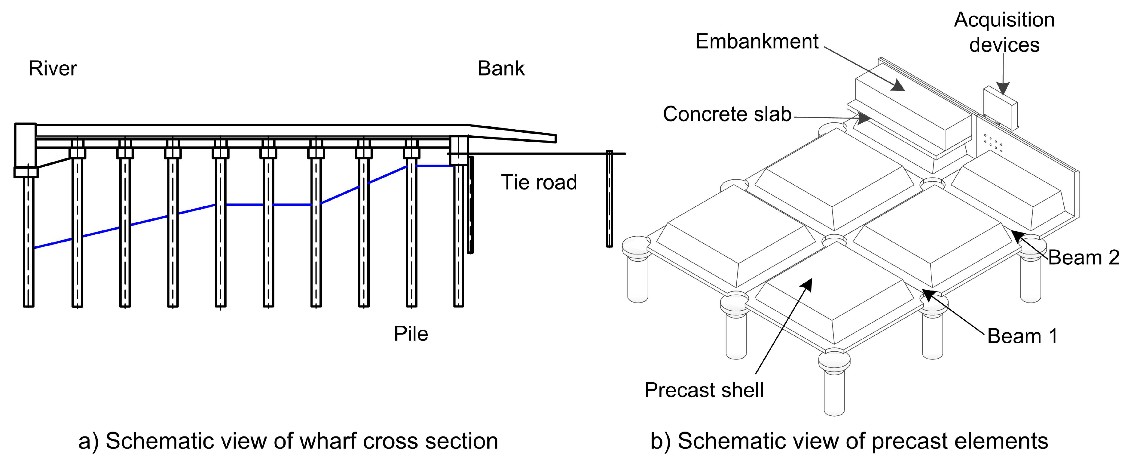
2.1. The Structure

The wharf is a 350 m long, 50 m wide on pile structure. It is composed of partly precast reinforced concrete elements. Precast parts are supported by a mesh of 579 steel piles distributed over 10 longitudinal rows and 56 transverse rows. Depending on the areas of the wharf, different service loads for parcel storage (offshore wind turbine nacelles) are planned (6, 10 or 15 ton/m 2 ) as well as crane tracks. The reinforced concrete platform is covered with a layer of embankment and asphalt. The platform is also equipped with bollards and berths. To stabilize the banks on which the platform is built, concrete inclusions and a system comprising a double sheet pile wall and tie rods have been installed (see Figure 1). The construction took over two years for a cost of around 40 million Euros and was achieved at the end of 2017.
The precast elements are concrete shells. They are embedded in the heads of steel piles (see Figure 1 and Figure 2).
The structural elements of the wharf called “beams” are delimited by the volumes between the prefabricated shells. Reinforcements are installed in this volume and then it is filled with concrete during the construction phase. Two structural elements located at the end of the platform are equipped with sensors (see Figure 1b and Figure 3).

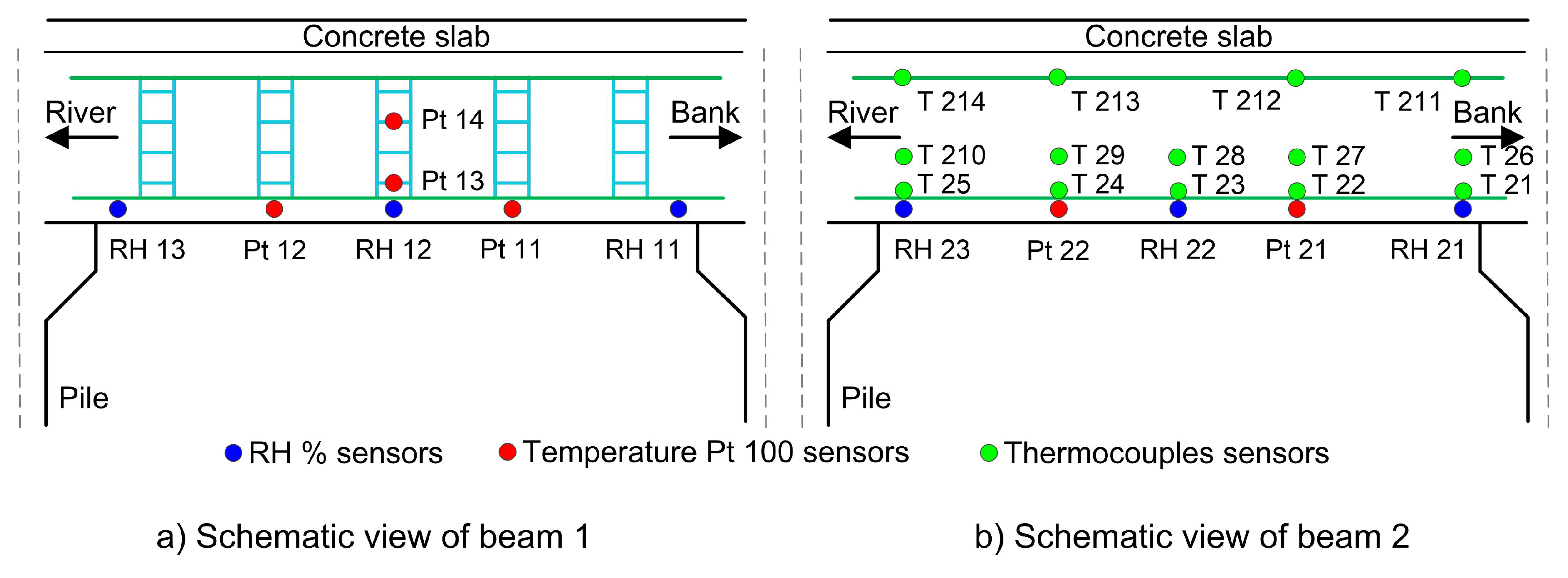
2.2. Technology and Positioning of the Sensors

The two beams in the instrumented zone are equipped with a multi-sensor system for monitoring chloride ion penetration and ageing according to the drawings in Figure 4.
Each beam is equipped with:
  • 2 resistivity sensors of the same technology as those used in [11];
  • 3 chloride sensors (physicochemical sensors with 3 electrolyte levels);
  • 3 sensors for the measurement of Direct Current (DC) electrical potential of reinforcement bars;
  • 3 combined humidity and temperature probes;
  • 6 Temperature probes Pt 100 and 14 thermocouples;
  • 2 optical fibers for simultaneous measurement of strain and temperature with a Brillouin—Rayleigh optical fiber interrogator.
These sensors are selected to measure changes in concrete related to the aging of the structure. Electrical DC resistivity measurement aims to detect the penetration of chloride ions into the concrete cover [12,13,14,15]. The resistivity depends on the porosity of the concrete, the water content, the concentration of chloride ions in the electrolyte and the temperature of the medium. Resistivity sensors are therefore used in combination with humidity and temperature sensors. Chloride sensors are designed to detect the front of chloride ion when it first reaches the reinforcement. The objective is to detect the presence of chloride before the corrosion process begins. DC electrical potential measurement is then used to predict the initiation of corrosion, before cracking appears. Finally, optical fibers are used to localize concrete cracking due to thermal changes or corrosion. This instrumentation is deliberately redundant in order to be able to compare the performance of the sensor technologies in the long term.
The Pt 100 probes and thermocouple sensors have been calibrated in temperature chambers. Humidity sensors were placed in temperature chambers in sealed containers containing saturated saline solutions according to standard [16]. The resistivity sensors were calibrated in a homogeneous medium including the actual reinforcement bars (see Figure 5) as described in Section 3.2.
Beam 1 (see Figure 4) is also equipped with 15 optical fiber extensometers (see Figure 6). Extensometers are positioned according to the symmetry plane of the beam at different distances of the neutral fiber. The objective of the strain measurements is to understand the actual behavior of the structural element. Because of its proportions, its behavior no longer falls within the validity domain of beam theory. Strain gauges are combined with strain-free Bragg gratings to measure temperature. The entire chain is calibrated by performing heating and cooling cycles in a thermal chamber.
Thermocouple or Pt 100 temperature sensors are positioned near resistivity sensors and strain gauges. They are used for the compensation of thermal effects on strain and resistivity measurements. Thermocouples, used in large numbers due to their low cost, are used to measure thermal gradients. The sensors whose data are analyzed in the following are marked on Figure 7.
The references of the sensors used and the names of the suppliers are listed in Table A1 in the Appendix A.

2.3. Acquisition Device

Data acquisition for chloride, temperature, potential and humidity sensors is carried out with a NI cDAQ-9133 acquisition unit which includes several acquisition cards. The central acquisition unit records:
  • Voltages from chloride sensors with an accuracy (for the acquisition device only) of 10 nV,
  • Thermocouple data: after thermocouple calibration and cold junction compensation, the maximum temperature uncertainty given by the thermocouples over the measuring range [−20 C; 40 C] is 0.9 C (defined as maximum to minimum deviation).
  • Voltages from temperature and humidity sensors with a maximum temperature uncertainty over the measuring range [−20 C; 40 C] of 0.25 C. The humidity measurement uncertainty over the same range is 1%.
  • Data from platinum resistance thermometers of type Pt 100 whose maximum temperature uncertainty over the measuring range [−20 C; 40 C] is 0.2 C.
The acquisition unit requires a 24 V DC power supply. It has been connected to an autonomous circuit. The 24 V DC came from batteries regularly replaced and connected to the acquisition unit via a converter, ensuring stable DC voltage during the initial connection of the installation. In a second stage, photovoltaic panels of about 0.5 m 2 were installed, in order to provide a maximum power of about 100 W.
The acquisition unit has an embedded operating system. It has a 2 GB memory and offers the possibility to connect an SD card. A Labview-coded program was developed in laboratory to record data from all the acquisition cards simultaneously at a desired frequency. The data is recorded on an SD card connected to the control unit. The acquisition of the signals of the Bragg grating optical fiber sensors (FBG) during the first months is carried out punctually with a portable device (HBM FS42 Portable BraggMETER). The resistivity measurement is carried out punctually with a resistivimeter ABEM terrameter LS, which is used as standard by geophysicists and is suitable for civil engineering applications [11,17].
The whole installation (batteries, electronics, central unit, etc.) allowing data acquisition has been integrated into waterproof boxes to protect it from external aggressions (wind, rain, tide, etc.). The boxes are positioned at the end of the platform as shown in Figure 3 and Figure 4.

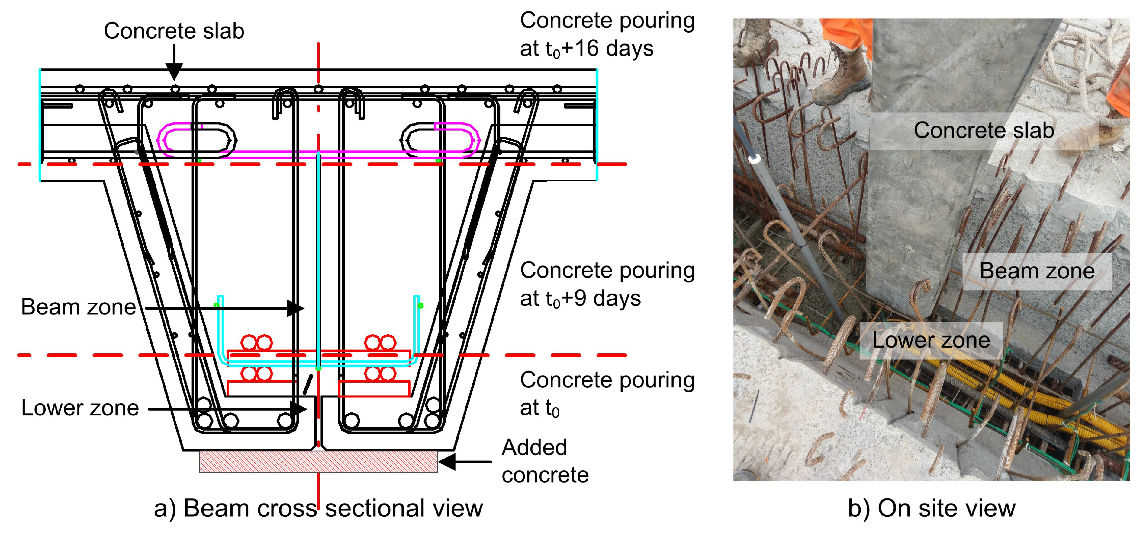
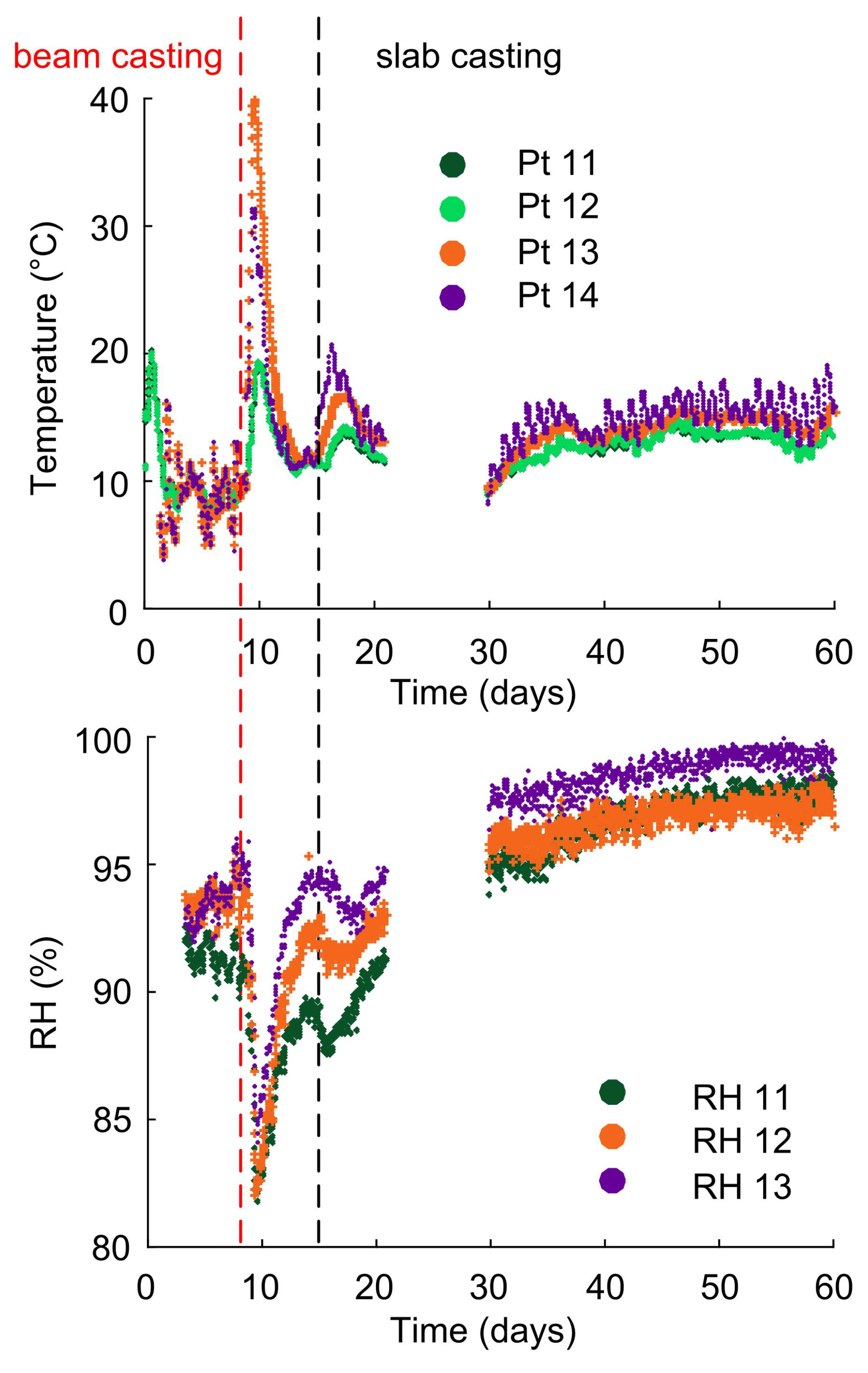
2.4. Construction Program

The installation of the measuring chain was carried out in conjunction with the progress of the construction works according to the following program:
  • t 0 - 3 days, the precast concrete shells are positioned on the pile heads;
  • t 0 - 3 days < t < t 0 , the reinforcement bars are placed in the lower part of the precast concrete shell in parallel with the installation of the sensors dedicated to corrosion measurement;
  • t = t 0 , the concrete is poured in the lower area (zone of resistivity sensors). Data acquisition is started at time t 0 ;
  • t 0 < t < t 0 + 2 days, the reinforcement bars are placed in the beams in parallel with the installation of the strain measurement sensors;
  • t = t 0 + 9 days, the concrete is poured at the junction of the concrete shells to form the beams;
  • t = t 0 + 16 days, the concrete slab is poured over the concrete shell.
The different areas listed above are shown in Figure 8 and limited by dashed red lines.

2.5. Materials and Mixture Used on Site

The composition of cast-in-place concrete is given in Table 1. The strength class was C40/50 and the mixture complied with the requirements of French Standard NF EN 206-1 for XA2 exposure class; i.e., minimum binder content of 350 kg/m 3 and maximum Effective water to Binder (Weff/Beq) ratio of 0.50. Portland cement CEM I 52.5 N SR3 was used to provide sulfate resistance. The actual Weff/Beq ratio was 0.45.

2.6. Material Tests Performed in Laboratory

In parallel with in-situ measurements, material tests were performed in controlled laboratory conditions in order to characterize the concrete used in the beams. On site, during the casting of the beams, 40 cylindrical samples of 110 mm diameter and 220 mm height, and one concrete prism of 70 × 70 × 280 mm 3 were also made with the same concrete. After one day, they were stored in water at 3 different temperatures: 4 were stored at 10 C, 4 at 40 C and the other at 20 C in order to perform maturity analysis and to determine activation energy. These samples were used to perform the following measurements:
  • Porosity accessible to water;
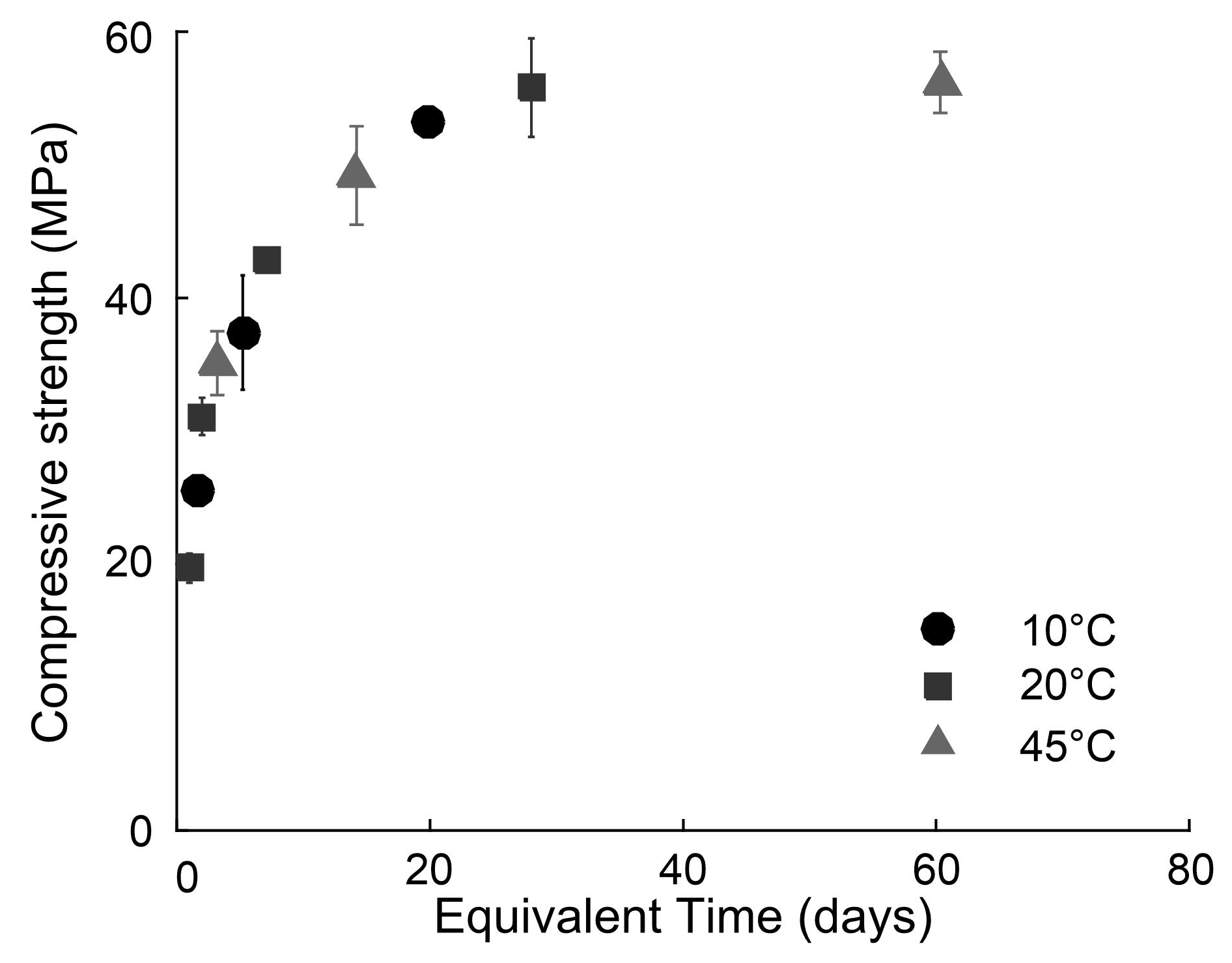
  • Compressive strength, (Maturity method [18]);
  • Elastic modulus.
Moreover, the same day, a piece of the concrete poured in the beam was taken and brought to the laboratory in less than one hour, in order to cast a 7 × 7 × 28 cm 3 specimen used to measure the autogenous deformation [19].

2.6.1. Porosity

An essential characteristic of reinforced concrete is its porosity since the pore structure has a strong influence on the diffusivity of chloride ions in concrete. It is therefore a determining factor in the durability of concrete [20]. After 90-day wet curing, water porosity P(%) was assessed on three concrete discs by the vacuum water saturation method, according to French standard NF P18-459 [21]. It is then deduced from mass measurements and Equation (1):
P = M sat - M d M sat - M w
where M sat is the mass of saturated sample in air, M d is the mass of oven-dried sample and M w is the mass of saturated sample in water.

2.6.2. Compressive Strength and Elastic Modulus

The compressive strength was assessed after 1, 2, 7, and 28 days on the specimens stored in water at different temperatures. Three specimens for each storage temperature were tested at each age. A non-destructive method based on the frequency of vibration was used to monitor the evolution of elastic properties on the set of specimens stored at 20 C. The natural frequencies of the concrete cylinders were measured with the Grindosonic equipment. The elastic modulus E was deduced by using the Spinner and Tefft model [22].

2.6.3. Autogenous Deformation

Autogenous deformation has been defined as the bulk deformation of a closed, isothermal, cementitious material system not subjected to external forces [23]. It mainly results from the hydration of cement. As studied concrete is located in the central part of the beam and in a relatively wet environment, drying is not expected to have a significant influence (at least during the presented study). Thus the laboratory monitoring consisted in measuring the length variations of 7 × 7 × 28 cm 3 specimen in sealed conditions. The sample was casted in laboratory with concrete taken on the construction site one hour before. After 24-h sealed curing at 20 C, the specimen was removed from formwork and immediately covered with a double-layer of adhesive aluminum tape. The autogenous deformation was monitored during one year. The mass-loss did not exceed 0.2% of initial mass.

3. Post-Treatment of Data for Comparison and Analysis

3.1. Analysis of Strain Measurement Performed with Fiber Bragg Gratings

Extensometer with Bragg grating optical fiber provides a Bragg wavelength λ 0 . The offset Δ λ with respect to a reference state is linked to thermal and mechanical strain. According to Equation (2):
Δ λ λ 0 = 1 - n eff 2 2 p 12 - ν f ( p 11 + p 12 ) ε + ξ Δ t
where Δ t is temperature change, ε is the axial strain of the FBG, n eff is the effective index of the mode propagating in the core of the fiber, ν f is the Poisson coefficient of the fiber, p 11 and p 12 are photo-elastic coefficients while ξ is the thermo-optic coefficient. Equation (2) can also be written in a condensed form:
Δ λ λ 0 = K ε + ξ Δ t
The value of K is given by the sensor supplier in the calibration report. According to Ferdinand [24], ξ = 1 n eff d n eff d T 7 × 10 - 6 K - 1 . It has been evaluated by thermal calibration for each sensor. In addition to the strain measurements, strain-free FBGs are positioned between top and middle levels (see Figure 6) to ensure thermal compensation of the system. During the first days, the relevant information that can be calculated using these extensometers is the shrinkage of the concrete at the core of the structure. It is calculated from the Equation (4) knowing the thermal dilatation coefficient of the concrete α concrete (with α concrete = 10 × 10 - 6 / C)
ε = α concrete Δ T + ε shrinkage

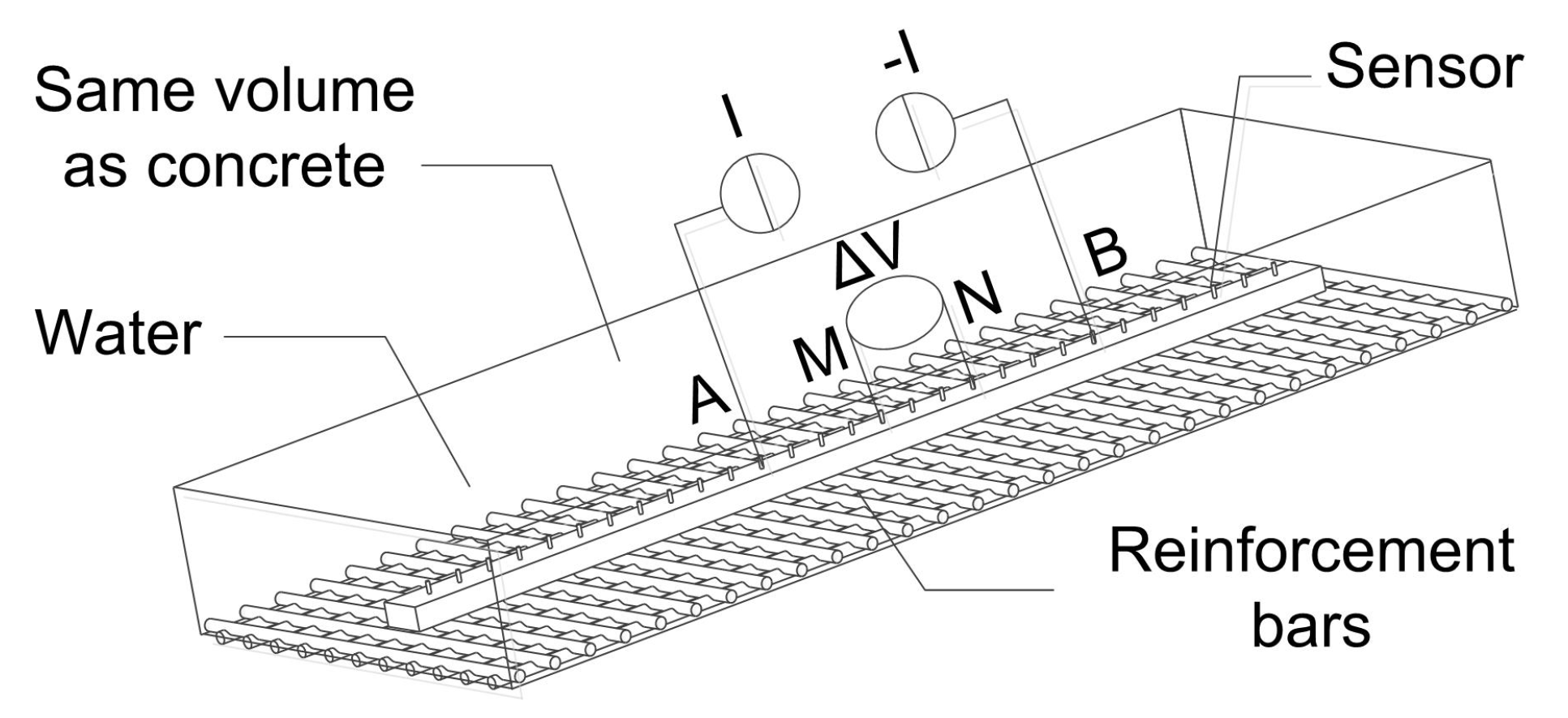
3.2. Analysis of Resistivity Measurement Performed with a Multi Electrodes Wenner Probe Embedded in Concrete

Concrete resistivity is measured in this study by electrical tomography. The resistivity noted ρ ( Ω . m ) , quantifies the propagation in a medium of an electric current I (A) continuously injected by an electrode embedded in concrete (see Figure 9). The usual electrical prospecting devices generally consist of two injection electrodes (A and B) and two electrodes M and N, allowing the measurement of the potential difference Δ V . The apparent resistivity for a 4-electrodes system is computed as follows:
ρ a = G Δ V I
G (m - 1 ) is the geometric factor that can be analytically calculated for a semi-infinite medium. For a Wenner [25] device as shown in Figure 9 and used for concrete beam monitoring, the inter-electrode distance is AM = MN = NB = a (with a = 25 mm). The sensor used on the wharf has 32 electrodes. Using a Wenner sequence of 4 electrodes [11,17], 129 different measurements can be carried out. Thanks to these measurements, a mapping of the apparent resistivities in a plane located under the sensor (called pseudo section of apparent resistivity) is obtained.
When the medium is of finite dimension such as studied beams, the geometric factor cannot be analytically computed (contrary to what is done in Geophysics [26]). Indeed, the latter depends on the geometry of the concrete beam and the reinforcement. As proposed by Du Plooy and al. [17], a numerical assessment of G was performed. The sensors have been calibrated in a homogeneous medium (here water of known resistivity) of the same volume as the concrete with reinforcement bars used on site (see Figure 5 and Figure 9).

3.3. Equivalent Age

Significant temperature gradients are likely to be generated in the studied beam due to dimensions of cross section of the wharf structural elements [27]. Early-age thermal cracks result from either differential expansion within a concrete element during heating causing internal restraint or by external restraint due to contraction during cooling stage. The main parameters involved in early age thermal cracking, i.e., strength, modulus, shrinkage, and creep, depend on concrete temperature history. Maturity method [18] allows estimating the properties of concrete from the measured temperature evolution of in-place concrete and laboratory tests in controlled conditions. This method is based on the measurements performed at different times of the compressive strength of the samples stored at different temperature (see Section 2.6.2). First, the evolution of the compressive strength of the samples stored at 20 C is fitted with a function adapted from the mathematical expression given in Eurocode 2:
f c T ref = f c 28 d e s 1 - 28 t
where f c 28 d is the compressive strength measured at 28 days, T ref = 20 C is the reference temperature and s is the adjustable parameter. In Eurocode 2 (NF EN 1992-1-1, 2005 [28]), the coefficient s takes into account the type of cement, from rapid hardening cements to low heat cements:
  • 0.20 for cements CEM 42.5 R, CEM 52.5 N, and CEM 52.5 R (Class R);
  • 0.25 for cements CEM 32.5 R, CEM 42.5 N (Class N);
  • 0.38 for cements CEM 32.5 N (Class S).
In the paper the coefficient s was adjusted to fit the actual strength development of the studied concrete. The value s = 0.21 was chosen to obtain the exact value of the strength measured at 2 days (see Table 2). The value is consistent with the intervals of Eurocode. The evolution of the compressive strength of the samples stored at 20 C serves as a reference. The underlying idea of the maturity method is to superimpose the evolutions of compressive strength with time at temperature T to this reference with the help of an equivalent age:
f c T ( t ) = f c T ref ( t e q ( T ) )
Equivalent age is the duration when concrete has to be stored at temperature in order to reach the same level of maturity as it would reach in the curing conditions defined by the temperature history T ( t ) . The influence of temperature on cement hydration and related properties can be taken into account through Arrhenius equation and activation energy E a . This allows calculating the equivalent age t e q from the Equation (8), given by Freiesleben Hansen et Pedersen [29]:
t e q ( T ) = 0 t e - E a R 1 T ( τ ) - 1 T ref d τ
where t e q is the equivalent age at reference temperature (days), E a is the apparent activation energy [J/mol], R is the gas constant 8.314 J/mol·K and T is the average absolute temperature of concrete [K]. E a is often referred to as “apparent activation” energy as hydration is the combination of several physical and chemical phenomena overlapping in time, thus it does not show a constant value [30,31]. However, for defined ranges of hydration degrees (or strengths) it can be assessed as a single value. In this study the apparent activation energy was determined using the method of superposition which consists in adjusting the value of activation energy E a , through Equations (7) and (8), in order to superpose the evolutions with time of the compressive strengths measured at 10 C and 45 C with the reference evolution over an interval [ f c min ; f c max ] . The value of E a has been calculated by the method of least squares in order to provide the best overlap of the data sets corresponding to the three testing temperatures.
First the equivalent age of the three sets of specimens was assessed for the different temperatures of 10, 20, and 45 C. The specimens were stored at 20 C during the first 24 h thus their common equivalent age at this time was 1 day. Then their equivalent ages were calculated using Equation (8). The values are given in Table 2. Their strengths at these equivalent ages were determined using Equation (6), with parameters f c 28 d = 55.8 and s = 0.21, as equivalent age is the duration when concrete has to be stored at reference temperature (here 20 C) to reach the same level of maturity. The value of E a R ratio was adjusted to minimize the differences between the measured strength and the calculated strength at each equivalent age. The values given in the Table 2 correspond to the best fit obtained with E a R = 2936 K. The highest strength value of 56.2 MPa at t e q = 60 days was not taken into account as the method is not well suited for predicting the evolution of hydration and strength at long-term.

4. Results and Discussion

4.1. Assessment of the Operability of the Embedded Sensors

The installation of a measuring system on a construction site in a moist environment is a challenging task. The risks of failure, particularly of the connectors, are significant. After the end of the construction stage, the number of defective sensors continues to increase. Failures are mainly caused by short circuits (leaking connections [26]). For the installation carried out on the on pile wharf, an assessment of the sensors in operation after one year is summarized in Table 3.
In the resistivity sensor “partially operable” (RS 12), short-circuits occurred between some electrodes. These short-circuits are easy to identify since they give negative potentials or values close to zero. So they reduce the number of useable sequences of measurement and consequently induce an increase in the measurement error of the average resistivity.
The optical fiber partially operable is broken, so the light cannot be transmitted from one end to the other. This means that it cannot be interrogated using the amplified Brillouin scattering method which is the most sensitive Brillouin method. However, it can be probed by reflection from each end by Brillouin optical time domain reflectometry or optical Rayleigh back scattering.
In addition to the sensors broken during installation, the number of operational sensors will decrease over the years for many reasons. The life expectancy of the embeddable chloride depth electrode is certified 10 years as well as the reference electrode type Silver/Silver, Chloride/Potassium. Indeed, these sensors will stop working when all reagents are consumed.
For the other sensors, their life expectancy in a corrosive environment is not known. The estimation of the life expectancy of each sensor will be an important result of this project. However, the following events can be assumed:
  • the filters of the humidity sensors may become clogged, preventing measurement (particularly due to the presence of chlorides);
  • before this deadline, since these probes require recalibration every 2 years, the risk is that the sensor signal drifts slowly;
  • Thermocouples type K and PT 100 probes are also susceptible to losing their calibration.
The drift of the measurements is a critical phenomenon since the measured temperature seems a priori correct. The drift of thermocouple measurements is, among other things, the result of the diffusion of atmospheric or metallic particles in thermocouple metals, most often caused by high temperatures. In the case of installation on a port wharf, the probable causes of measurement drift will be corrosion and strain-hardening of the sensors. These phenomena will also affect PT100 probes.
Finally, aberrant measures are likely to be recorded on all electrical sensors. Let us take the example of reference electrodes, These sensors should not normally be affected by external conditions since these sensors are designed to be embedded. However, the cable lengths are about 10 m and the measured potentials very low. Even with shielded cables, the low signal-to-noise ratio can have a negative influence on the measurement. Being able to identify sensors that provide incorrect information will be a major issue in this project for years to come.
Conversely, a long service life is expected for Bragg grating strain sensors. Since the information is coded in wavelength and not in amplitude, the signal should not drift. The measurement will therefore be usable as long as the optical fiber is mechanically protected by the stainless steel cladding. Thus, for future structural monitoring projects in harsh environments, it is expected that sensors based on fibre optic technologies will largely replace electrical sensors once the technology is available and affordable. This is, for example, what is emerging in the context of application to the monitoring of nuclear waste storage structures [32].

4.2. Material Parameters

The porosity of the concrete used on site was 12%. This porosity value is relatively low [20] and in line with the class of concrete used during construction.
In this research, the interval [ f c min ; f c max ] chosen to determine the activation energy, following Equation (8) was [29 MPa; 54 MPa]. Data are analyzed after the first 24 h during which all specimens are stored at the same temperature. Figure 10 and Figure 11 show the time-temperature transformation based on the calculation of equivalent age. The bars on the graph correspond to the standard deviation of experimental measurements.
The highest strength of 56.2 MPa resulted from 28-day curing at 45 C. The value of activation energy deduced from the superposition method was 24.4 kJ/mol. This value was used to assess equivalent time for the specimens cured at 10 C and 45 C on the graph of Figure 11.
Activation energy can be used to estimate concrete properties such as strength, modulus, and to a certain extent autogenous shrinkage [33,34] at different locations of the studied beam from their temperature history measured in situ and the activation energy determined from compressive tests in laboratory (Figure 11). Yikici et al. [35] compared the strengths predicted by the maturity method and the actual strength measured on drilled cores. The predicted strength values were comparable to the core strength. Equations (6)–(8) have been used to assess the evolution of actual strength in the beam from the evolution of the actual temperature T ( t ) (Figure 12). The Pt 14 sensor is located in the center on the beam, Pt 11 at the bottom (Figure 7). The difference between both strength evolutions in relatively low, which is in line with relatively low temperature gradients measured across the section of the beam.
The evolution of Young’s modulus provided by dynamic testing is plotted on the graph of Figure 13.
Although this method is known to overestimate this property [36], the experimental results show relatively high values of elastic modulus from the age of 1 day, which suggests that relatively low shrinkage or thermal strains are likely to generate significant stresses from early-age. Consequently, the shrinkage values and thermal gradients measured on site require a careful monitoring and analysis in relation to the mechanical resistances and the evolution of the modulus of elasticity.

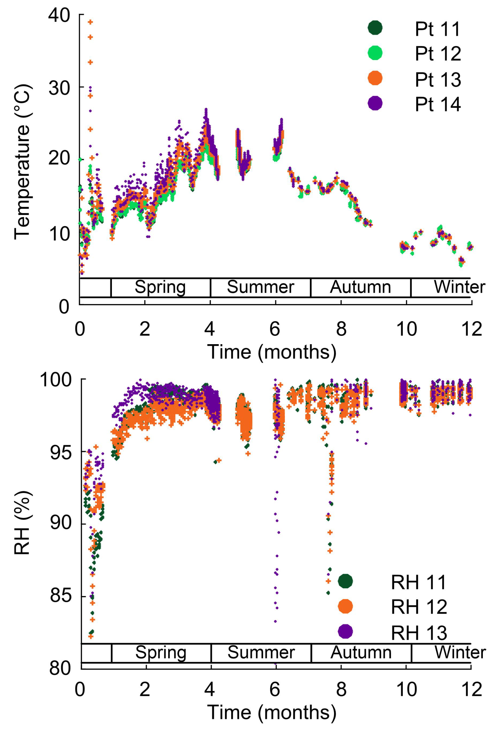
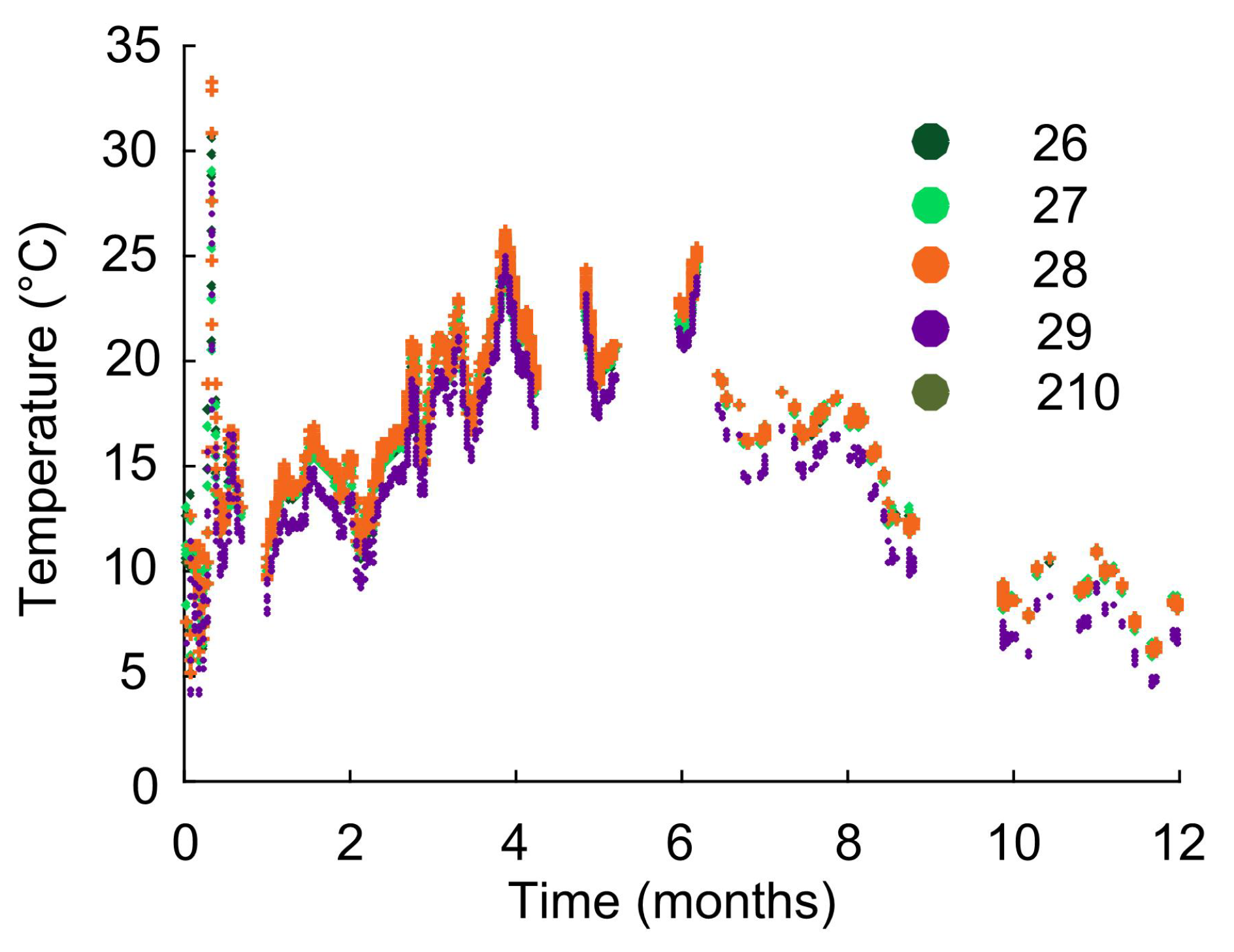
4.3. In Situ Measurement of Relative Humidity and Temperature

The on-site temperature measurement is a mean for evaluating, the risks of cracking at early age, or the time required before removing the formwork [37,38]. In the present study, temperature measurement is an input for maturity method. Another use is the correction of the sensors’ measurements, all sensitive to temperature (resistivity, strain and rebar potential). The different stages of the construction process are visible on the temperature evolution during the 60 first days (see Figure 14). The first peak on day 0 recorded by the two low level probes (Pt 11 and Pt 12) corresponds to the casting of the lower part of the beam. The second with a peak at 40 C for Pt 13 (and 30 C for Pt 14) corresponds to the casting of the central zone of the beam that affects also the temperature of the lower zone (peak at 20 C). Finally, the peak at 16 days corresponds to the pouring of the slab.
Figure 15 gives the evolution of temperature during the first 12 months. Daily variations (day-night cycle) and seasonal variations are visible respectively on Figure 14 and Figure 15. However, there is no visible variation linked to the tidal cycle.
High temperature at early age must be avoided as it is likely to trigger cracking during the first days and delayed ettringite formation at long term. Note that here the maximum temperature during beam casting did not exceed 40 C. Above 48 C, ettringite produced by the hydration of cement becomes less stable than monosulfate [39]. Thus the maximum temperature reached in the beam did not affect the stability of the main hydration products and delayed ettringite formation will be avoided [40]. Figure 14 also shows that the temperature gradients across the beam are acceptable in terms of thermal cracking mitigation. The maximum difference recorded between center and surface temperatures in beam 2 was approximately 10 C, which is low enough to prevent cracking due to internal restraint [41]. The measurements provided by the sensors thus confirm that the design of construction sequence was relevant to mitigate the pathologies due to temperature increase in concrete at early-age.
On the same beam, the relative humidity measured in concrete in the lower zone is shown in Figure 14 and Figure 15.
Recording began 48 h after the concrete was poured. The humidity probes are positioned at 80 mm depth in concrete openings recapped immediately after insertion of the sensors. It is therefore a measure of the relative humidity inside a cavity of a few cubic centimeters (about 10 cm 3 ) in the concrete. This is not a direct measure of water content in the porosity. The relation between relative humidity measurement and concrete degree of saturation is not direct. It is given by the sorption-desorption isotherm of the studied concrete (see for example the studies of Harmathy [42] and Baroghel-Bouny [43]). Obtaining these curves requires maintaining samples in a controlled environment (RH% and T C) until the mass of the sample has stabilized and then gradually varying the relative humidity of the ambient air. These measurements are not complex but require several months or years of testing since the time required to stabilize the samples is very long. This time is comparable to hydration characteristic times thus both phenomena are coupled during the period of interest, and it is not possible to deduce the water saturation from relative humidity measurements since casting time. The desorption curves published in the literature show that a concrete subjected over the long term to a very humid environment (between 98 and 100% of relative humidity) is nearly saturated with water. Several factors actually influence concrete saturation, mainly hydration and external drying. Given the water-to-cement ratio of 0.45 (see Table 1), free water remains in the pores even after the complete hydration of cement [44]. The decrease of relative humidity in concrete due to external drying is a relatively slow phenomenon, even at a depth of a few centimeters (see [45]). Given the stability of RH over the long term (here between 98% and 100% of relative humidity), the RH of studied beam was still not affected by external drying. The underside elements of the structure are regularly submerged or splashed during tidal cycles. A decrease of this relative humidity to 95% after four months corresponds to the summer season with higher temperature in concrete (see Figure 15 where the 5th month corresponds to the beginning of July 2017).The relatively humidity in concrete bean was actually affected by the diffusion of heat as the decreases of relative humidity can be correlated with temperature peaks (see Figure 15). Although it is not possible to state that concrete is saturated with water only on the basis of a relative humidity measurement in a cavity, the water saturation of concrete is likely very high. This assumption is consistent with the low resistivity values measured on site (see Section 4.5) while the porosity is low (see Section 4.2). The underside elements of the structure are regularly submerged or splashed during tidal cycles which probably explains this relative humidity value in the concrete.
Alternative measurement methods could also have been used to directly measure the degree of saturation of a given concrete after a calibration operation. Resistivity measurement is an example, but capacitance probes or Time-Domain Reflectometer (TDR) probes can also be mentioned. The disadvantage of these technologies lies in their sensitivity to pollutants, particularly chlorides.

4.4. Strain Measurement

The shrinkage measurements (considering correction of thermal effect and equivalent age of concrete) are presented for the sensors located on the middle level in Figure 16. The extensometer supporting frame 1 is near the bank and the 5 on the river side (see Figure 6). For the sensors of the high and low level, plots are given in the appendix because the trends are similar. The mean value of each level is also considered for analysis. Similar shrinkage rates can be observed for the different levels (low, middle and top in Appendix B). The shrinkage was systematically higher in the center of the beam, in the most massive part. In absence of service loading, the strain measurement could appear of fair interest. Nevertheless, after taking into account the temperature evolution and once associated with the results of the material tests (modulus, strength, shrinkage in laboratory), shrinkage is one of the main parameters affecting the risk of cracking at early age.
The strain of concrete at 20 C in laboratory conditions has been plotted on Figure 16 and Figure 17 as a function of equivalent time. This takes into account the influence of measured temperature on equivalent age of concrete (see Section 3). Equivalent age is often used to predict the actual strength of concrete knowing its temperature history. This concept has been used for the prediction of autogenous shrinkage [33]. These authors actually showed that maturity can be used for isothermal and realistic conditions as long as temperatures remain between 10 and 40 C. The conditions of the evolution of the structural concrete can be considered as similar to autogenous shrinkage as the relative humidity in concrete remained close to 100% (see Figure 14 and Figure 15). This allowed the hydration of cement to continue, thus the observed shrinkage was mainly due to self-desiccation. The strains obtained from laboratory experiments are of the same order of magnitude as the values determined from the measurements on the construction site. The 100 μ m/m is the typical magnitude of the autogenous shrinkage of normal strength concrete.
In both series of results (laboratory and in situ) a slight swelling can be observed during the first 20 days. This cannot be attributed to thermal dilation as the peak due to hydration appeared much earlier. Casting took place at 8.9 days and the temperature actually came back to casting temperature at 11.7 days (Figure 14). This swelling has already been observed in previous experimental studies [46]. This could be due to the rapid growth of hydration products at early age and the resulting crystallization pressure exerted on the pore walls [47,48,49].
Sensors located on the supporting frame 3 showed higher deformation. They were located in the center of the beam, where the temperature increase was the highest according to the measurement performed in beam 2 (see Figure 18). Peak temperature was 34 C in the center and between 27 and 31 C in the four other locations (see Figure 7 and Figure 18). The temperature decrease causes the buildup of tensile stresses due to the increase of elastic modulus during concrete hardening, and the restraint is higher in the central part, thus higher tensile stress could be expected at frame 3. The higher values given by sensors located on the supporting frame 3 would result not only from material parameter related to autogenous shrinkage, but also from structural effect. The evolutions of the deformations at the four other locations were averaged and plotted on the same graph on Figure 17 as the deformation measured in the laboratory. Both series of data are globally in good agreement. Lower values are given by the sensors located at the top of the beam. This can be interpreted by the effect of compressive load induced by bending.

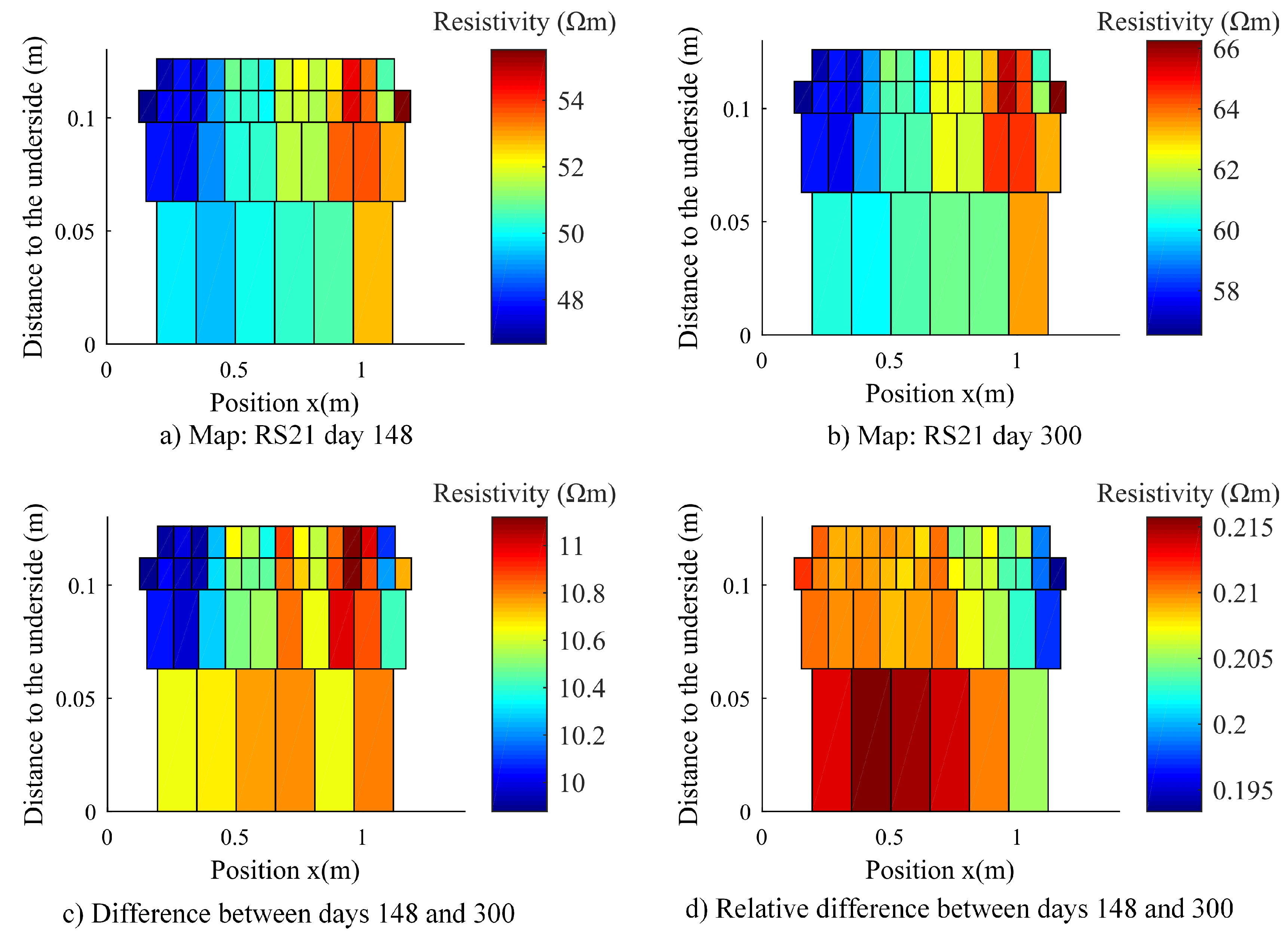
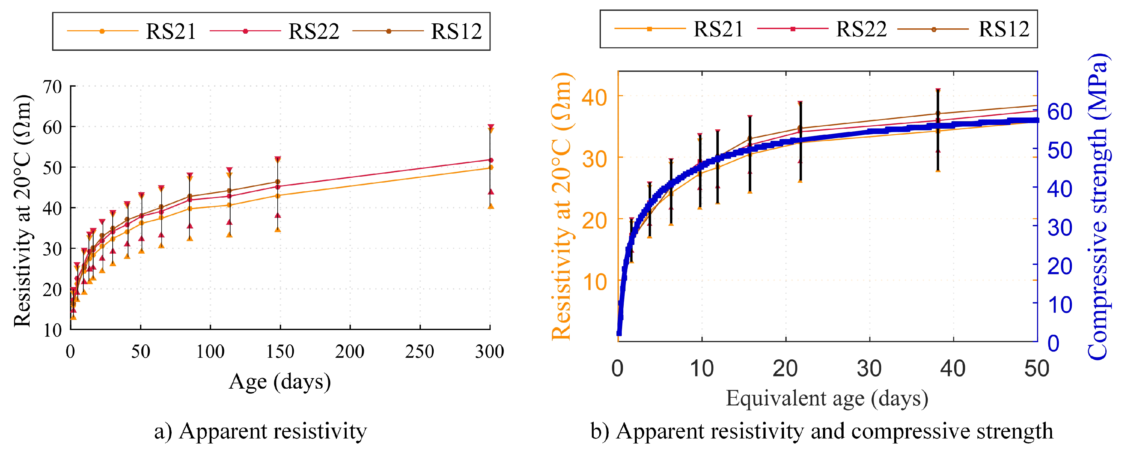
4.5. Measurement of Apparent Resistivity

Resistivity measurement is plotted on a map of apparent resistivity of the area between the sensor and the surface exposed to the sea. Figure 19 presents an example of resistivity map measured in beam 1 with sensor RS21, respectively 148 and 300 days after casting in concrete. In this case, the resistivity is about 51 Ω ·m with erratic variations between 47 Ω ·m and 55 Ω ·m for the measurement performed the day 148 while it is about 62 Ω ·m with erratic variations between 57 Ω ·m and 66 Ω ·m for the measurement performed the day 300.
The apparent resistivity depends mainly on the temperature, the porosity of the medium, the electrolyte content of the pores and the conductivity of the porous solution. By comparing the pseudo section measured at different dates, it will be possible to detect a drop in resistivity and the probable progress of a chloride front. An example is provided in Figure 19b,c. In this case the difference is positive, which indicates a possible drying of the concrete.
At early age, the chloride ions have not significantly penetrated inside the beams. The spatial dispersion of measured resistivity is mainly due to the heterogeneity of the material. It is then reasonable within the framework of process monitoring to use the mean value of the measured resistivity as the value of the global resistivity of concrete. An example is given for beam 1 in Figure 20. Each point on this curve represents the average of the 129 resistivity values measured on site at a given equivalent age (according to the computation explained in Section 3.3). The error bar represents the standard deviation of the resistivity values around the average value of the measurements taken for a sensor. Finally, since the resistivity changes with temperature, a thermal correction was performed to compute the resistivity for the reference temperature T ref = 20 C according to Equation (9):
ρ T mes = ρ T ref 1 + α T mes - T ref
where ρ T mes is the apparent resistivity measured at the temperature T mes and ρ T ref is the apparent resistivity computed for the temperature T ref . Finally, α is the correction factor of temperature effects. In this study, the coefficient is set at 0.022 C - 1 as proposed by Whittington and al. [50].
The corrected curves are shown on Figure 20a. With the thermal correction, the curves are similar to those describe by the authors who performed resistivity measurement in laboratory on concrete specimens, most often with Wenner portable devices [13,51]. This result validates the relevance of the measurements obtained with the in-situ device. Moreover, the two sensors embedded in beam 2 (RS21 and RS 22) about 20 cm apart and 1 m long each, give almost the same average values.
As shown in Figure 20b, there is a strong correlation between resistivity and compressive strength evolution. The resistivity of concrete is dependent on many factors, e.g., pore structure, pore solution, temperature and degree of water saturation. However, for a given concrete (same chemical composition), whose degree of saturation remains stable and after a correction of thermal variation on measurement, the only variable parameter is the porosity. In this study, it is reasonable to consider that the degree of hydration changes only slightly (see the value of RH% always close to 100% during the first year of structure service life). Additionally, it is recognized that the strength of concrete is mainly determined by porosity instead of other factors, e.g., pore solution and water saturation. Since the porosity evolves with hydration [52] thus modifying the resistivity value and the mechanical strength of concrete, the resistivity measurement can be considered as an indicator of material hardening. As a consequence, when the resistivity has reached its asymptotical value, it is probable that compressive strength is close to the maximum.

4.6. Discussion

The analysis of the experimental data collected in-situ shows that to obtain exploitable information, it is necessary to analyze simultaneously measurements from the various sensors and the results of tests carried out in laboratory. With the exception of temperature, data from a single type of sensor does not contain information that can be used directly to monitor manufacturing processes. An example is the strain measurement. Combined with temperature measurement and material testing, it can detect areas where concrete shrinkage is likely to cause cracking of the structure at early age. It is easier to estimate the behavior of concrete from laboratory tests. The humidity measurements performed in situ confirmed that the shrinkage was mainly due to self-desiccation, thus laboratory tests in sealed conditions can be considered as relevant.
In addition to the simultaneous analysis of several measurands, it is important to underline the importance of the measurement history. The knowledge of the initial state of each sensor is particularly crucial. This is the case, for example, for calculating concrete shrinkage based on strain measurements. More generally, a continuous or regular measurement is easier to interpret than a punctual measurement giving the state of the structure. Whenever possible, it is therefore interesting to start data acquisition before concreting.
The resistivity measurement provides another illustration. In the scientific literature, a threshold value is retained as an indicator of corrosion. The probability of initiation of corrosion is considered high for a value of 100 Ω ·m [13]. Within the wharf, on a new structure, and after several months of measurement, the resistivity is still below this threshold. As explained above, since concrete is not very porous, only a high water content of the material, due to the location of the structure (on the riverside) can explain this measure. To have relevant information on the evolution of the corrosion risk and to be able to detect the progress of the chloride front in a particular area, the exploitable information is the relative difference between two states [53], i.e., between two pseudo sections of apparent resistivity as presented in Figure 19. If this relative difference shows a decreasing resistivity value near the surface of the structure, one possible conclusion is that it is caused by the penetration of a chloride front. A strong correlation was observed between increased resistivity and mechanical strength. The study of Liu et al. [54] actually showed that after the de-percolation time of capillary pores, the resistivity of cement paste is controlled by the volume fraction of C–S–H, which is also the main hydration product for its contribution to mechanical strength. The measurement of resistivity could thus be used as part of material monitoring. The “ageing factor” which characterizes the time evolution of the chloride diffusion coefficient can be determined from resistivity measurements on saturated specimens [55]. The resistivity has the advantage of being a non-destructive technique, thus it allows a continuous monitoring in the same specimen (laboratory) or at the same location of a structure (in-situ). The maturity analysis and the determination of activation energy allow correlating the evolutions of strength, resistivity, and temperature.

5. Conclusions

This article relates the instrumentation with a multi-sensor measurement chain of a wharf in Saint-Nazaire, France. The structural health monitoring system had two objectives: on the one hand, to contribute to feedback on the operation of the structure in service and, on the other hand, to extend the service life of the structure. The monitoring started in the instrumented area at the same time as the in-situ concreting. The analysis of the parameters assumed as the most sensitive to concrete changes, and therefore to the manufacturing process, was thus carried out during the first months of the structure’s life thanks to the following sensors:
  • Fiber optic extensometers (FBG);
  • Pt 100 and thermocouple sensors;
  • Relative humidity sensors;
  • Embedded resistivity sensors.
These measurements were supplemented by material testing in the laboratory: 40 samples were casted with the concrete used in the instrumented beams and submitted to several mechanical tests. The porosity of the concrete was found equal to 12%. Porosity value can be considered as low [20]. This is consistent with the use of high performance concrete with high mechanical strength. The compressive strength was close to 60 MPa after 50 days. The Young modulus was greater than 30 GPa after 1 day and tended to 45 GPa. Significant stress is likely to appear at early age due to this high value of Young Modulus, which reinforces the need for a careful monitoring. The construction sequence allowed mitigating the early-age thermal cracking as the maximum temperature and the thermal gradient did not exceed 40 C and 30 C respectively.
After one year, 53 sensors over 59 are fully operable, and 2 are partially operable. This has made possible a thorough characterization of the evolution of the structure at early stage. First of all, the relative humidity measured in small cavities inside the beams remains close to 98% during the first year. This slow evolution is probably due to the fact that the lower part of the wharf is cyclically submerged. The temperature exhibits a peak at 40 C in the center of the beams during casting. Then it is mainly driven by external temperature. Seasonal and daily variations were observed but no variation linked to the tidal cycle. The in-situ strain measurements show that the extremities of the beam experience a strain similar to the autogenous strain measured in laboratory, whereas the central part is twice strained. This higher value of strain is influenced by structural effects. At early age, the resistivity of the concrete is almost uniform and remains lower than 70 Ω ·m. This value is smaller than the value of 100 Ω ·m classically considered as the threshold value corresponding to high probability of corrosion. Beyond this risk of corrosion due to the environment of the structure, it will be interesting to compare the resistivity values at different times, to be able to identify a possible modification of the corrosion risk. Calculating the difference between two pseudo-sections of apparent resistivity will thus be a method allowing the detection of an area potentially contaminated with chloride ions. Moreover, it has been shown that the resistivity is a good indicator of material hardening. It indicates especially when the concrete has reached its long-term compressive strength.
The simultaneous start of the acquisition with concreting made it possible to validate the operation of the measuring chain and the identification of the malfunction of failed sensors. Analysis of the data at early age showed that strain and resistivity measurements could be directly exploited within the framework of manufacturing process monitoring. However, to be fully exploitable, these measurements must be combined with temperature measurements. Moisture measurements and material testing also provide interesting additional information for analysis. Strength measurements combined with the determination of activation energy, and the monitoring of resistivity, allow comparing the development of mechanical and physical concrete properties and showing their correlation.
The study presented here proposes a multi-physical database of in situ measurements or material tests collected during one year. The initial state of the structure and the material are therefore perfectly known. The data presented in this paper is meant to be updated within five to 10 years once the degradation process has begun. The knowledge of the complete measurement history will promote a better understanding of degradation processes. Additionally, the study shows that a measurement chain dedicated to the SHM could be a tool for validating the quality of the construction of a reinforced concrete structure. The measuring chain allows early detection of structural disorders, thus limiting the risk of costly repairs during the operating phase.
The data collected on site and the results of the material tests presented in this article are available in the Supplementary Materials. The aim is to propose a database to analyze the link between measurements carried out in laboratory with data recorded during the construction of a real structure.

Supplementary Materials

The Supplementary Materials are available online at https://www.mdpi.com/2077-1312/7/4/84/s1.

Author Contributions

Conceptualization, Y.L. and E.R.; Funding acquisition, F.S.; Investigation, M.C., V.G., R.G., Y.L., D.L., C.L., J.P. and E.R.; Project administration, Y.L. and F.S.; Writing—original draft; V.G., Y.L., D.L., J.P. and E.R.; Writing—review & editing M.C., C.L. and F.S.

Funding

This research was funded by the Pays de la Loire region within the framework of IMARECO2 project.

Acknowledgments

The authors would like to thank all the partners of iMAREO2 project: Keops Automation (D. Follut, D. Olivier), Université de Nantes (M. Roche), Nantes—Saint Nazaire Port (P. Lijour, M. Labegorre) and Bouygues Construction (the teams of Bouygues Travaux Publics Régions France). Special thanks are due to Thierry Giorgetti (acquisition unit installation) and Antoine Bassil (sensors installation) for their help in this project. The authors would like to thank the Pays de la Loire region for its financial support.

Conflicts of Interest

The authors declare no conflict of interest.

Appendix A. Sensor References

Table A1. Sensor used on site: references and suppliers.
SensorReferenceSupplier
Embedded Strain SensorFS62 length 100 mmHBM
Optical cableBRUsens DSS 2.8 mm V1 non-metallicSOLIFOS
T C and RH% probesHC2-C05ROTRONIC
PT 100 probeROF-PT100 Class AROTRONIC
Embeddable chloride depth electrodeCP80C-Probe Systems
Reference electrodeCP10P ElectrodeC-Probe Systems
Silver/Silver Chloride/Potassium

Appendix B. Strain Measurement in Laboratory and Beam 1

Figure A1. Strain measurement in concrete during concrete shrinkage for the whole sensors. (a) Strain measurement in the top level; (b) Strain measurement in the middle level; (c) Strain measurement in the bottom level.
Jmse 07 00084 g0a1aJmse 07 00084 g0a1b

References

  1. Boero, J.; Schoefs, F.; Capra, B.; Rouxel, N. Technical management of French harbour structures—Part 1: Description of built assets. Rev. Paralia 2009, 2, 6.1–6.11. [Google Scholar] [CrossRef]
  2. Boero, J.; Schoefs, F.; Capra, B.; Rouxel, N. Technical management of French harbour structures—Part 2: Current practices, needs—Experience feedback of owners. Rev. Paralia 2009, 2, 7.1–7.12. [Google Scholar] [CrossRef]
  3. von Wolffersdorff, P. Workshop Sheet Pile Test Karlsruhe; Technical Report; Delft University: Delft, The Netherlands, 1994. [Google Scholar]
  4. Finno, R.J.; Roboski, J.F. Three-Dimensional Responses of a Tied-Back Excavation through Clay. J. Geotech. Geoenviron. Eng. 2005, 131, 273–282. [Google Scholar] [CrossRef]
  5. Del Grosso, A.; Lanata, F.; Brunetti, G.; Pieracci, A. Structural health monitoring of harbour piers. In Proceedings of the 3rd International Conference on Structural Health Monitoring of Intelligent Infrastructure, Vancouver, BC, Canada, 13–16 November 2007. [Google Scholar]
  6. Catbas, F.N.; Aktan, A.E. Condition and Damage Assessment: Issues and Some Promising Indices. J. Struct. Eng. 2002, 128, 1026–1036. [Google Scholar] [CrossRef]
  7. Delattre, L.; Duca, V.; Sherrer, P.; Rivière, P. Anchoring efforts on Osaka quay wall at LeHavre harbour. In Geotechnical Engineering for Transportation Infrastructure; Balkema, A.A., Ed.; A.A. Balkema: Rotterdam, The Netherlands, 1999; Volume 2, pp. 713–718. [Google Scholar]
  8. Schoefs, F.; Yáñez-Godoy, H.; Lanata, F. Polynomial Chaos Representation for Identification of Mechanical Characteristics of Instrumented Structures. Comput. Aided Civ. Infrastruct. Eng. 2011, 26, 173–189. [Google Scholar] [CrossRef]
  9. Schoefs, F.; Le, K.T.; Lanata, F. Surface response meta-models for the assessment of embankment frictional angle stochastic properties from monitoring data: An application to harbour structures. Comput. Geotech. 2013, 53, 122–132. [Google Scholar] [CrossRef] [Green Version]
  10. Liu, H.B.; Zhang, Q.; Zhang, B.H. Structural health monitoring of a newly built high-piled wharf in a harbor with fiber Bragg grating sensor technology: Design and deployment. Smart Struct. Syst. 2017, 20, 163–173. [Google Scholar] [CrossRef]
  11. Lecieux, Y.; Schoefs, F.; Bonnet, S.; Lecieux, T.; Lopes, S.P. Quantification and uncertainty analysis of a structural monitoring device: Detection of chloride in concrete using DC electrical resistivity measurement. Nondestruct. Test. Eval. 2015, 30, 216–232. [Google Scholar] [CrossRef]
  12. Saleem, M.; Shameem, M.; Hussain, S.E.; Maslehuddin, M. Effect of moisture, chloride and sulphate contamination on the electrical resistivity of Portland cement concrete. Construct. Build. Mater. 1996, 10, 209–214. [Google Scholar] [CrossRef]
  13. Polder, R.B. Test methods for on site measurement of resistivity of concrete—A RILEM TC-154 technical recommendation. Construct. Build. Mater. 2001, 15, 125–131. [Google Scholar] [CrossRef]
  14. Morris, W.; Vico, A.; Vazquez, M.; de Sanchez, S.R. Corrosion of reinforcing steel evaluated by means of concrete resistivity measurements. Corros. Sci. 2002, 44, 81–99. [Google Scholar] [CrossRef]
  15. Andrade, C.; d’Andrea, R.; Rebolledo, N. Chloride ion penetration in concrete: The reaction factor in the electrical resistivity model. Cem. Concr. Compos. 2014, 47, 41–46. [Google Scholar] [CrossRef]
  16. AFNOR. Mesure de l’Humidité de l’air—NF X15-119; Technical Report NF X15-119; AFNOR: Paris, France, 1999. [Google Scholar]
  17. du Plooy, R.; Palma Lopes, S.; Villain, G.; Dérobert, X. Development of a multi-ring resistivity cell and multi-electrode resistivity probe for investigation of cover concrete condition. NDT E Int. 2013, 54, 27–36. [Google Scholar] [CrossRef]
  18. LCPC. Guide Technique La Résistance du Béton Dans L’ouvrage; Technical Report; LCPC: Chapel Hill, NC, USA, 2003. [Google Scholar]
  19. Samouh, H.; Rozière, E.; Wisniewski, V.; Loukili, A. Consequences of longer sealed curing on drying shrinkage, cracking and carbonation of concrete. Cem. Concr. Res. 2017, 95, 117–131. [Google Scholar] [CrossRef]
  20. Baroghel-Bouny, V. Conception Des Bétons Pour une Durée de Vie Donnée des Ouvrages; Technical Report; Association Française de Génie Civil: Paris, France, 2004. [Google Scholar]
  21. AFNOR. Essai Pour Béton Durci —Essai de Porosité et de Masse Volumique—NF P18-459; Technical Report NF P18-459; AFNOR: Paris, France, 2010. [Google Scholar]
  22. Spinner, S.; Tefft, W. A Method for Determining Mechanical Resonance Frequencies and for Calculating Elastic Moduli from These Frequencies; ASTM: West Conshohocken, PA, USA, 1961; pp. 1221–1238. [Google Scholar]
  23. Jensen, O.M.; Hansen, P.F. Autogenous deformation and RH-change in perspective. Cem. Concr. Res. 2001, 31, 1859–1865. [Google Scholar] [CrossRef]
  24. Ferdinand, P. Capteurs à Fibres Optiques à Réseaux de Bragg. Available online: https://www.techniques-ingenieur.fr/base-documentaire/mesures-analyses-th1/cnd-methodes-surfaciques-42586210/capteurs-a-fibres-optiques-a-reseaux-de-bragg-r6735/ (accessed on 27 March 2019).
  25. Wenner, F. A method of measuring earth resistivity. J. Wash. Acad. Sci. 1915, 5, 561–563. [Google Scholar] [CrossRef]
  26. Barker, R. Depth of investigation of collinear symmetrical four-electrode arrays. Geophysics 1989, 54, 1031–1037. [Google Scholar] [CrossRef]
  27. Lanata, F.; Schoefs, F. Multi-algorithm approach for identification of structural behavior of complex structures under cyclic environmental loading. Struct. Health Monit. 2011. [Google Scholar] [CrossRef]
  28. CEN. NF EN 1992-1-2—Octobre 2005—Calcul des Structures en béton—Partie 1-1: Règles Générales et Règles Pour les Batiments; Technical Report; CEN: Bruxelles, Belgium, 2005. (In French) [Google Scholar]
  29. Freiesleben Hansen, P.; Pedersen, E. Maleinstrument til Kontrol af betons haerdning. Nordisk Betong 1977, 1, 21–25. [Google Scholar]
  30. D’Aloia, L.; Chanvillard, G. Determining the “apparent” activation energy of concrete: Ea—Numerical simulations of the heat of hydration of cement. Cem. Concr. Res. 2002, 32, 1277–1289. [Google Scholar] [CrossRef]
  31. Carette, J.; Staquet, S. Monitoring and modelling the early age and hardening behaviour of eco-concrete through continuous non-destructive measurements: Part I. Hydration and apparent activation energy. Cem. Concr. Compos. 2016, 73, 10–18. [Google Scholar] [CrossRef]
  32. Piccolo, A.; Lecieux, Y.; Delepine-Lesoille, S.; Leduc, D. Non-invasive tunnel convergence measurement based on distributed optical fiber strain sensing. Smart Mater. Struct. 2019, 28, 045008. [Google Scholar] [CrossRef]
  33. Turcry, P.; Loukili, A.; Barcelo, L.; Casabonne, J.M. Can the maturity concept be used to separate the autogenous shrinkage and thermal deformation of a cement paste at early age? Cem. Concr. Res. 2002, 32, 1443–1450. [Google Scholar] [CrossRef]
  34. Kamen, A.; Denarié, E.; Sadouki, H.; Brühwiler, E. Evaluation of UHPFRC activation energy using empirical models. Mater. Struct. 2009, 42, 527–537. [Google Scholar] [CrossRef]
  35. Yikici, T.A.; Chen, H.L.R. Use of maturity method to estimate compressive strength of mass concrete. Const. Build. Mater. 2015, 95, 802–812. [Google Scholar] [CrossRef]
  36. Neville, A. Properties of Concrete, 5th ed.; Prentice Hall: Englewood Cliffs, NJ, USA, 2011. [Google Scholar]
  37. American Concrete Institute. Cold Weather Concreting—ACI 306R; Technical Report ACI 306R; American Concrete Institute: Detroit, MI, USA, 2002. [Google Scholar]
  38. American Concrete Institute. Standard Specification for Cold Weather Concreting—ACI 306; Technical Report ACI 306; American Concrete Institute: Detroit, MI, USA, 2002. [Google Scholar]
  39. Lothenbach, B. Thermodynamic equilibrium calculations in cementitious systems. Mater. Struct. 2010, 43, 1413–1433. [Google Scholar] [CrossRef]
  40. Collepardi, M. A state-of-the-art review on delayed ettringite attack on concrete. Cem. Concr. Compos. 2003, 25, 401–407. [Google Scholar] [CrossRef]
  41. Bamforth, P.B. Early-Age Thermal Crack Control in Concrete; CIRIA: London, UK, 2007. [Google Scholar]
  42. Harmathy, T. Effect of Moisture on the Fire Endurance of Building Elements. Moisture Mater. Relat. Fire Tests 1965. [Google Scholar] [CrossRef]
  43. Baroghel-Bouny, V. Caractérisation Microstructurale et Hydrique des Pâtes de Ciment et des Bétons Ordinaires et à Très Hautes Performances. Ph.D. Thesis, Ecole Nationale des Ponts et Chaussées, Paris, France, 1994. [Google Scholar]
  44. Powers, T.C. A discussion of cement hydration in relation to the curing of concrete. Highw. Res. Board Proc. 1948, 27, 178–188. [Google Scholar]
  45. Samouh, H.; Rozière, E.; Loukili, A. The differential drying shrinkage effect on the concrete surface damage: Experimental and numerical study. Cem. Concr. Res. 2017, 102, 212–224. [Google Scholar] [CrossRef]
  46. Lura, P. Autogenous Deformation and Internal Curing of Concrete; Delft University Press: Delft, The Netherlands, 2003. [Google Scholar]
  47. Sellevold, E.; Bj øntegaard, O. Driving forces to cracking in hardening concrete: Thermal and autogenous deformations. In Proceedings of the 2nd International Symposium on Advances in Concrete through Science and Engineering, Quebec City, QC, Canada, 11–13 September 2006. [Google Scholar]
  48. Darquennes, A.; Staquet, S.; Delplancke-Ogletree, M.P.; Espion, B. Effect of autogenous deformation on the cracking risk of slag cement concretes. Cem. Concr. Compos. 2011, 33, 368–379. [Google Scholar] [CrossRef]
  49. Darquennes, A.; Rozière, E.; Khokhar, M.I.A.; Turcry, P.; Loukili, A.; Grondin, F. Long-term deformations and cracking risk of concrete with high content of mineral additions. Mater. Struct. 2012, 45, 1705–1716. [Google Scholar] [CrossRef]
  50. Whittington, H.W.; McCarter, J.; Forde, M.C. The conduction of electricity through concrete. Mag. Concr. Res. 1981, 33, 48–60. [Google Scholar] [CrossRef]
  51. Brameshuber, W.; Dauberschmidt, C.; Schröder, P.; Raupach, M. Non-Destructive Determination of the Water Content in the Concrete Cover Using the Multi-Ring-Electrode; Technical Report RWTH-CONV-006116; DGZfP: Potsdam, Germany, 2003. [Google Scholar]
  52. Burlion, N.; Bourgeois, F.; Shao, J.F. Effects of desiccation on mechanical behaviour of concrete. Cem. Concr. Compos. 2005, 27, 367–379. [Google Scholar] [CrossRef]
  53. McCarter, W.J.; Chrisp, T.M.; Starrs, G.; Basheer, P.A.M.; Blewett, J. Field monitoring of electrical conductivity of cover-zone concrete. Cem. Concr. Compos. 2005, 27, 809–817. [Google Scholar] [CrossRef] [Green Version]
  54. Liu, Z.; Zhang, Y.; Jiang, Q. Continuous tracking of the relationship between resistivity and pore structure of cement pastes. Const. Build. Mater. 2014, 53, 26–31. [Google Scholar] [CrossRef]
  55. Andrade, C.; Castellote, M.; d’Andrea, R. Chloride aging factor of concrete measured by means of resistivity. In Proceedings of the Proceedings of the XII-International Conference on Durability of Building Materials and Components, Porto, Portugal, 12–15 April 2011. [Google Scholar]
1.
https://www.cost-tu1402.eu (November 2014–April 2019).
Figure 1. Schematic view of the wharf.
Jmse 07 00084 g001
Figure 2. The wharf during construction (precast shell elements and metal piles).
Jmse 07 00084 g002
Figure 3. Zone of interest.
Jmse 07 00084 g003
Figure 4. Location of potential, chloride and resistivity sensors (referenced RS i).
Jmse 07 00084 g004
Figure 5. View of reinforcement bars and resistivity sensors for on-site measurement (bottom view).
Jmse 07 00084 g005
Figure 6. Instrumentation for strain measurement (beam 1).
Jmse 07 00084 g006
Figure 7. Temperature and humidity sensors in beam 1 and beam 2.
Jmse 07 00084 g007
Figure 8. Identification of zones of the structure cast at different times.
Jmse 07 00084 g008
Figure 9. Principle of measurement and schematic view of the experimental set-up.
Jmse 07 00084 g009
Figure 10. Influence of curing temperature on compressive strength.
Jmse 07 00084 g010
Figure 11. Compressive strength as a function of equivalent time.
Jmse 07 00084 g011
Figure 12. Modelling of concrete compressive strength evolution in beam 1.
Jmse 07 00084 g012
Figure 13. Elastic modulus of concrete specimens stored at 20 C.
Jmse 07 00084 g013
Figure 14. Temperature and relative humidity measured in beam 1 during the first two months.
Jmse 07 00084 g014
Figure 15. Temperature and relative humidity measured in beam 1 during the first year.
Jmse 07 00084 g015
Figure 16. Temperature (dashed red line), strain of structural concrete in the middle level of frames 1 to 5 and strain at the material scale from laboratory measurement (solid black line).
Jmse 07 00084 g016
Figure 17. Temperature (solid red line), average strain over four frames of structural concrete at the top, middle and bottom levels of the frames (average value of extensometers located on the supporting frames 1, 2, 4 and 5) and strain at the material scale from laboratory measurement (solid black line).
Jmse 07 00084 g017
Figure 18. Measurement of the temperature using thermocouples sensors in beam 2 at the locations of the strain sensors on beam 1.
Jmse 07 00084 g018
Figure 19. Example of pseudo section of apparent resistivity measured in beam 1 by sensor RS 11, 148 days after casting in concrete (a), 300 days after casting in concrete (b,c) is the difference between the two pseudo sections of resistivity and (d) the relative difference.
Jmse 07 00084 g019
Figure 20. Evolution of the average value of the apparent resistivity computed at 20 C vs concrete age [0–300 days] (a) and apparent resistivity computed at 20 C vs. concrete equivalent age [0–50 days] (b) plotted with evolution of compressive strength. Error bars represent the standard deviation σ of measurements.
Jmse 07 00084 g020
Table 1. Composition of concrete mix.
ComponentContent (kg/m3)
Gravel 11/22740
Gravel 2/10300
Sand 0/4810
Cement CEM I 52.5 N SR3 (C)360
Plasticizer3.8
Water effective161
Table 2. Determination of apparent activation energy from compressive strengths.
AgeEquivalent AgeStrength f c T Strength f c T ref ( t eq ( T ) )
Temperature t t eq
(Equation (8))
Compression TestingComputation
(Equation (6)
10 C1119.722.3
21.725.629.1
75.2137.442.1
2819.9553.253.6
20 C1119.722.3
2231.131.1
7742.845.1
282855.855.8
45 C1119.722.3
23.235.136.8
714.1949.251.2
2860.3656.259.7
Table 3. Sensors in operation.
Type of SensorNumber of Embedded SensorsNumber of Sensors in Operation
FBG for strain measurement1513 (2 broken wires)
Resistivity42 with measurements fully available
1 with measurements partially available (water in connections)
1 inoperable
RH%65 (broken wire)
Pt 10066
Reference electrode Ag+66
Chlorides66
Optical fiber for strain and temperature measurement (crack detection)21 fully operable
1 partially operable
Thermocouples1414

