Cavitation Prediction of Ship Propeller Based on Temperature and Fluid Properties of Water

Abstract

Cavitation is a complex phenomenon to measure, depending on site conditions in specific regions of the Earth, where there is water with various physical properties. The development of ship and propulsion technology is currently intended to further explore territorial waters that are difficult to explore. Climate differences affect the temperature and physical properties of water on Earth. This study aimed to determine the effect of cavitation related to the physical properties of water. Numerical predictions of a cavitating propeller in open water and uniform inflow are presented with computational fluid dynamics (CFD). Simulations were carried out using Ansys. Numerical simulation based on Reynolds-averaged Navier–Stokes equations for the conservative form and the Rayleigh–Plesset equation for the mass transfer cavitation model was conducted with turbulent closure of the fully turbulent K-epsilon (k-ε) model and shear stress transport (SST). The influence of temperature on cavitation extension was investigated between $0 \mathrm{and} 50 \text{°}\mathsf{C}$. The results obtained showed a trend of cavitation occurring more aggressively at higher water temperature than at lower temperature.

1. Introduction

Along with the development of technology, the development of transportation facilities for people and logistics can be done quickly at large scale. The shipping and maritime sector also cannot be separated from technological developments in the context of exploration in new potential areas. The opening of the Northern Sea Route (NSR) for ship transportation, which connects the Atlantic and Pacific Oceans through the Arctic Sea, presents opportunities for ocean exploration and shipping line efficiency [1,2]. Vessels, as a means of sea transportation, must be designed following the terrain to be traversed, to improve ship performance and shipping safety [3,4]. It is known that climate differences on Earth affect the characteristics of the water in the ocean, so there is a need for comprehensive research on the performance of ships to overcome these conditions.

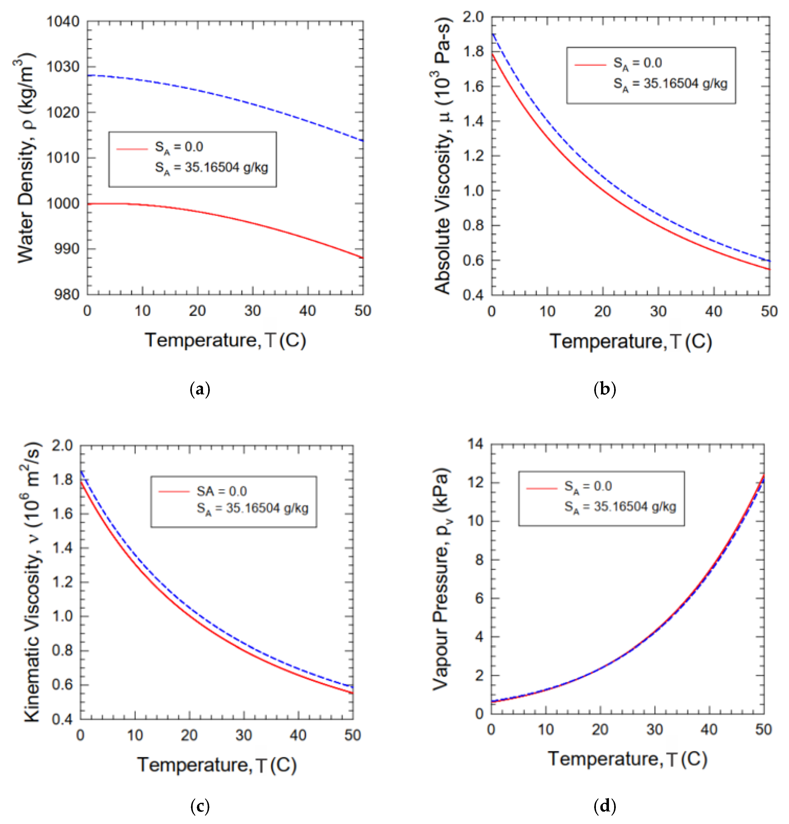
Cavitation is one of the severe problems that occur in every marine application. The basic theory of fluid mechanics says that every object that moves in a fluid will be impacted by the influence of viscosity, even more if the object is operating at high speed. Ship propellers, as part of ship propulsion systems that interact directly with water at high speed, are the most prone to erosion due to cavitation. Cavitation is a phenomenon in which vapor forms in low-pressure regions of freestream fluid. Bursting cavitation bubbles cause pitting of the blade surfaces. Substantively, the most extensive problem caused by cavitation is the material damage when the bubbles burst near the propeller surface, an undesirable occurrence [5]. Inception from small empty cavities develops, and they expand to larger size. The formation and disappearance of the vapor phase in liquid happens when the local pressure drops below the saturated vapor pressure. During the cavitation process, the fluid fraction of both water and vapor will move to a higher pressure region. This makes the bubbles implode and generate an intense explosion [6]. Subsequently, the bubble cavities collapse near a solid surface, and they can cause material damage. Cavitation erosion has been recognized as a major problem in the engineering design and operation of high-speed flow systems, especially in turbomachinery. This phenomenon is a complex problem and requires a deeper understanding of the mechanism. Cavitation is also widely found in ship propellers. It is an important phenomenon because of the effect, which can cause component failure, reduced efficiency, vibration instability of operation, and noise. Decreased performance is characterized by cavitation, which can be seen from decreased propeller thrust and the torque produced [7]. Because of this, cavitation becomes a crucial parameter that must be considered in ship propulsion design, including its interaction with environmental conditions, e.g., water density, viscosity and vapour pressure (see Figure 1).

The background of this research also began with the study of the cavitation phenomenon in a pump, which has the same working principle as a rotating machine. Pumps are used in industry, for example, in oil processing plants. They can perform with different temperatures and different types of fluids. From some cavitation studies with variable fluid temperature and type of fluid in the pump, it is known that these variables affect the occurrence of cavitation. Sparker [9], with the collaboration of experiment and analytical calculation, found that additional reduction in net positive suction head (NPSH) for hydrocarbon compared with cold water NPSH. Alarabi [10], with experimental works, concluded that NPSH inception increases as temperature increases, reaching nearly 30 °C, then decreases with decreasing temperature, and increasing water temperature accelerates cavitation inception. Hosien and Selim [11] found that experimental and theoretical results had good agreement, and experimental results indicated that at low water temperature, breakdown blade cavitation number increased with increasing temperature. Jan Meijn [12], who used numerical CFX-TASCflow (AEA Technology, Waterloo, Canada) with constant enthalpy vaporization (CEV) model, found that different types of fluids greatly affect the growth pattern of cavitation bubbles, and stability of turbulent model is an important parameter to consider. Chivers [13], on other hand, who used numerical and experimental studies, noted that at higher operational water temperatures, total upstream head minus vapor pressure, which can be achieved, was lower. Based on the conclusions of all the studies, the authors were encouraged to apply various temperatures to predict the cavitation phenomenon on ship propellers. The temperature difference affects water and water vapor properties, as presented in Figure 1.

In this study, numerical prediction of cavitation flows over marine propeller was carried out. We investigated the flow around a model scale propeller called the Potsdam Propeller Test Case (PPTC), in this study PPTC model VP1304, in oblique flow. The simulations were validated with the available experimental data provided by the Schiffbau-Versuchsanstalt Potsdam (SVA) Propeller workshop (International Symposium on Marine Propulsors - SMP’15) [14]. The multi-phase flow was modeled with approaches to heat transfer. We assumed that the two phases are always in a thermodynamic equilibrium process. It can be considered that heat transfer occurs instantaneously and the phases are in perfect thermal contact. The mixture is an assumed homogenous model with total energy for the heat transfer process. All simulations were carried out using Ansys CFX (ANSYS Inc., Canonsburg, PA, USA) commercial computational fluid dynamics (CFD) solver. The simulation was carried out at a temperature range of $0 \mathrm{to} 50 \text{°}\mathsf{C}.$ Even though the water in the ocean does not reach $50 \text{°}\mathsf{C}$, this was intended to see the impact of temperature on cavitation more clearly. Because the nature of seawater is more complex, the physical properties of water were simplified by defining material properties based on the physical properties of freshwater. The physical property parameters, thermodynamic parameters, and transport properties were specified with values using the CFX-Pre user materials. To assess the influence of transition turbulent flow, first we used the shear stress transport (SST) with automatic wall treatment, then we applied the standard k-ε for the fully turbulent model with scalable wall function.

2. Literature Review

2.1. Numerical Method of Cavitation Phenomenon

Now, along with the advances in computational dynamics, several approaches for modeling flow physics have been developed. These approaches are the Reynolds-averaged Navier–Stokes (RANS) method, large eddy simulation (LES) technique, detached eddy simulation (DES), and direct numerical simulation (DNS). In 1999, Kunz et al. [15] obtained a prediction of cavitation on a propeller by computing two viscous flows with the RANS equation for multi-phase flow. In addition, Salvatore et al. used blade element momentum (BEM) to predict the performance of an Istituto Nazionale per Studi ed Esperienze di Architettura Navale (INSEAN) propeller in inviscid flow [16], modeling cavitating flow as a homogeneous mixture model of two fluids. The applied governing equations consist of momentum equations and continuity (volume) for the mixture of these fluids, along with a transport equation for the water volume fraction. The mass transfer rate due to cavitation uses the same equation. Modeling cavitation in CFX automatically uses the default mass transfer model presented by Zwart [17]. Kunz et al. [15] and Singhal et al. [18] also applied the mass transfer model for cavitating flow, known as the Kunz model and full cavitation model (FCM), respectively. The models were added to the CFX solver using CFX Expression Language (CEL), considering that the mass transfer model is needed to improve the accuracy and stability of numerical simulations by providing empirical coefficients to adjust the mass transfer rate due to evaporation and condensation [19]. Lungu [20] performed cavitation modeling on the PPTC model VP1304 using a numerical approach based on the finite volume method with the turbulent closure approach through Detached Eddy Simulation (DES). Regener [21] performed a numerical analysis of cavitation on propellers by considering the interaction of flow between the water and the ship’s hull. The non-uniform inflow to the propeller was simulated using the RANS method.

2.2. Related Research

Vapor formation is different from boiling because the process occurs at a more or less constant temperature, and the evaporation process is caused by lowering the pressure below the saturation pressure at a certain temperature. Cavitation can be defined as a thermodynamic change of phase with mass transfer from liquid to vapor phase, and bubbles will implode when the pressure increases [16]. It means that in the phase change between liquid and fluid, not only mass is transferred, but also heat is transferred between the phases from liquid to vapor. Brennen [19] explained that the phenomenon of cavitation occurs at a constant temperature, assuming that the process is at a thermodynamic equilibrium. These assumptions mean that the energy equation is important for a closed system. Rodio et al. [22] explained that the effect of temperature in a cavitation model that assumes isothermal processes must be added to other assumptions, to be in either thermal or non-thermal equilibrium. Assuming thermal equilibrium means that the temperature is the same for each liquid–vapor phase and the system is closed with regard to temperature. Thus, the assumption neglects the change in temperature at the interface between the two phases, while assuming no thermal equilibrium means that the phase interface has a temperature difference. The vapor bubbles absorb heat from the bulk liquid when cavitation occurs, so vaporization results in reduced temperature near the liquid–vapor interface. This phenomenon, called the thermal effect, delays the development of cavitation. Several studies have analyzed the thermal effect on cavitation by making model equations based on the Rayleigh–Plesset equation. Franc and Pellone [23] implemented a simple model to analyze the thermal effect in a cavitation inducer based on the Rayleigh–Plesset equation with convective and conductive approaches to model the heat transfer near the liquid–vapor interface. Viitanen et al. [24] simulated cavitation on a propeller in open water conditions. The simulation method was carried out assuming homogeneous and compressible flow for multi-phase flow. The combined approach of RANS and hybrid RANS/LES was applied. The results of the simulation using this approach provided a good picture of the cavitation pattern. In addition to numerical predictions, cavitation on propellers can also be observed experimentally. Pereira et al. [25] conducted experimental research to find out the relationship between the near pressure field and the cavitation pattern on an INSEAN E779A propeller. The experiments obtained accurate data, although there were limitations to the analysis.

Based on data from the International Association for the Properties of Water and Steam (IAPWS), the nature of water is a function of temperature $\left(S_A=0\right)$, pressure $\left(P\right)$, and absolute salinity ${(S}_A)$. The data in the IAPWS table is calculated based on one standard atmospheric pressure with variable temperature and salinity values in freshwater $\left(S_A=0\right)$ [8]. Sharqawy et al. [26] wrote that fluid is a single-phase thermodynamic system with variable physical properties based on mass, volume, pressure, temperature, and salinity. In this regard, temperature and salinity are the independent properties of heat and desalination, and most of the properties examined are given in the temperature range of $0$ to $120 \text{°}\mathsf{C}$ and salinity range of 0 to 120 g/kg. However, the surface tension data and correlations are limited to an oceanographic temperature range of $0$ to $40 \text{°}\mathsf{C}$ and salinity of 0 to 40 g/kg. Other parameters, such as thermal conductivity, specific heat capacity, and evaporation heat in seawater, have different values in freshwater. Latent heat, which has an important influence on the evaporation event between the water surface and water vapor, is also affected by the level of salinity. Unlike the nature of saltwater, the nature of freshwater is calculated at an absolute pressure of 1 atm (0.101325 MPa).

3. Propeller Model and Test Case

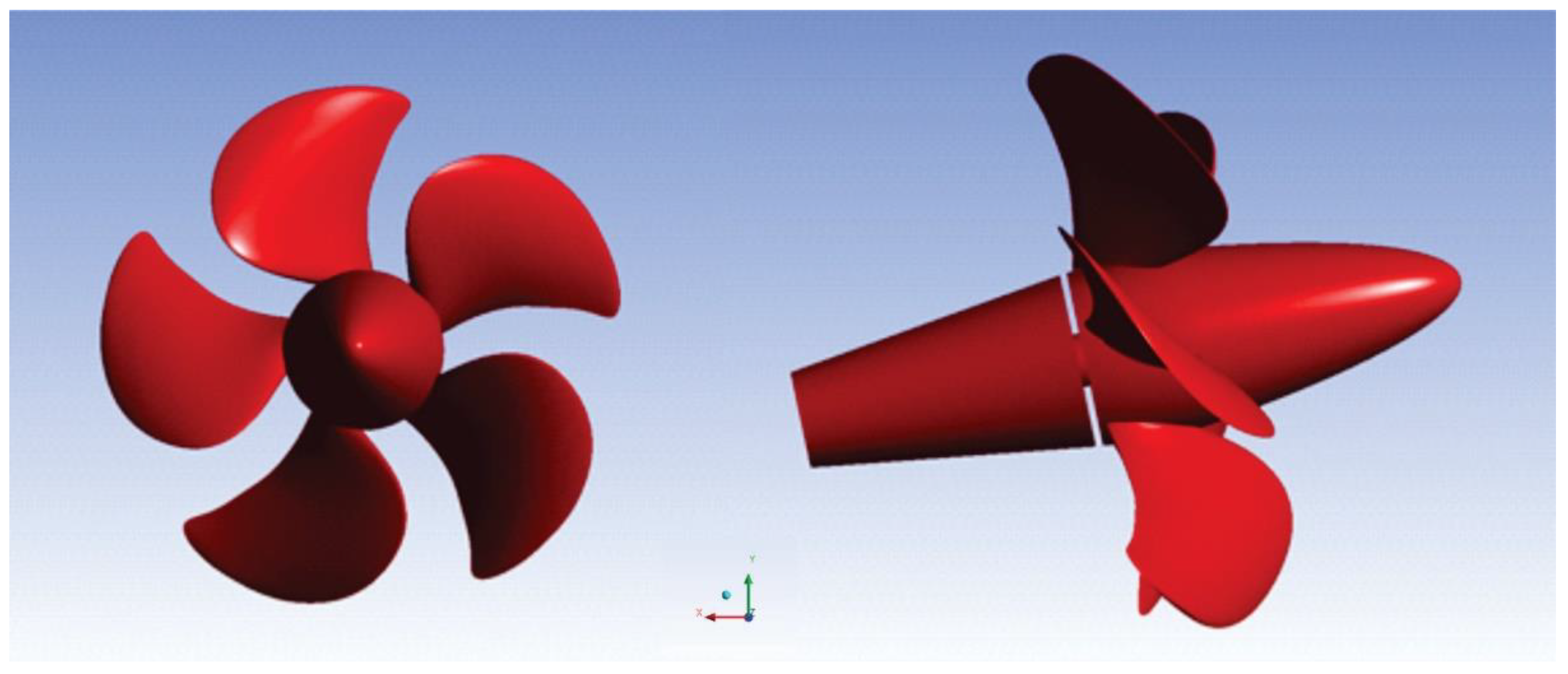
Schiffbau-Versuchsanstalt Potsdam (SVA) created a propeller design known as the PPTC1 model VP1304 for research and validation purposes. The experimental data and geometries are published on the company’s website (www.sva-potsdam.de/pptc). Previous research used the VP1304 model for numerical simulation and validation data, and it was used at the Fourth International Symposium on Marine Propulsors 2015 (SMP’15) [27]. The significant advancement of computer performance has made more numerical simulation possible. Numerical prediction of propeller performance under cavitating flows using CFD simulation has become a good alternative to experimental study. The VP1304 propeller was applied to simulation cases 1–3, displayed in

Table 1. Case properties.

Parameter	Symbol	Unit	Case 1	Case 2	Case 3
Advance Coefficient	$J$	-	1.019	1.269	1.408
Cavitation Number	${\sigma }_n$	-	2.024	1.424	2.000
Rotational Speed	$n$	rps	20	20	20
Saturated Pressure	$P_v$	$\mathrm{bar}$	0.029	0.029	0.029
Water Temperature	$T$	°C	23.7	23.7	23.7

. The 3D model was downloaded from the website. The VP1304 five-bladed, controllable pitch propeller has a right-handed direction of rotation (see Figure 2). The propeller has a pulling configuration positioned with $12\text{°}$ inclination toward the flow direction.

The simulation consisted of two case sections. First, the test case was the simulation of cavitating flow in existing conditions, used for validation. Fluid properties of water and vapor were set at a temperature of $23.7 \text{°}\mathsf{C}$. The physical properties used in numerical simulations assume that water is a pure substance. Saturation vapor pressure is the value of the reference temperature. This section consisted of three operational conditions, as shown in

Table 2. Overview of parameters used for observation.

Fluid	Unit	$0 \text{°}\mathbf{C}$	$12 \text{°}\mathbf{C}$	$25 \text{°}\mathbf{C}$	$37 \text{°}\mathbf{C}$	$50 \text{°}\mathbf{C}$
$P_v$	$\mathrm{bar}$	0.006	0.014	0.032	0.063	0.124
${\rho }_l$	${\mathrm{kg}/\mathsf{m}}^3$	999.793	999.452	997.004	993.294	988.009
${\rho }_v$	${\mathrm{kg}/\mathsf{m}}^3$	0.005	0.011	0.023	0.044	0.083
${\text{µ}}_l$	$\mathrm{Pa}. \mathsf{s}$	1.79 × 10−3	1.23 × 10−3	8.90 × 10−4	6.91 × 10−4	5.47 × 10−4
${\text{µ}}_v$	$\mathrm{Pa}. \mathsf{s}$	9.22 × 10−6	9.51 × 10−6	9.87 × 10−6	1.02 × 10−5	1.06 × 10−5
$h_l$	$\mathrm{kJ}/\mathrm{kg}$	−0.042	50.410	104.838	155.004	209.336
$h_v$	$\mathrm{kJ}/\mathrm{kg}$	2500.893	2522.886	2546.544	2568.173	2591.310
$s_l$	$\mathrm{kJ}/\mathrm{kg} \mathsf{K}$	−1.55 × 10−4	0.181	0.367	0.532	0.704
$s_v$	$\mathrm{kJ}/\mathrm{kg} \mathsf{K}$	9.156	8.851	8.557	8.313	8.075
$C_{p, l}$	$\mathrm{kJ}/\mathrm{kg} \mathsf{K}$	4.220	4.193	4.182	4.179	4.180
$C_{p, v}$	$\mathrm{kJ}/\mathrm{kg} \mathsf{K}$	1.888	1.898	1.912	1.928	1.948
${\alpha }_l$	$\mathsf{W}/\mathsf{m} \mathsf{K}$	0.561	0.584	0.607	0.626	0.644
${\alpha }_v$	$\mathsf{W}/\mathsf{m} \mathsf{K}$	0.017	0.018	0.019	0.019	0.020

Note: $P_v$ is fluid and vapor pressure at reference temperatures; ${\rho }_l$ is water density; ${\rho }_v$ is vapor density, ${\text{µ}}_l$ and ${\text{µ}}_v$ are dynamic viscosity of water and vapor; $h_l$, $h_v$, $s_l$, and $s_v$ are thermodynamic parameters consisting of enthalpy and entropy of liquid and vapor; $C_{p, l}$ and $C_{p, v}$ are isobaric heat capacity of fluids; and ${\alpha }_l$ and ${\alpha }_v$ are thermal conductivity of water and vapor.

.

Section 2 was the simulation as a case to be observed, i.e., the observation case. The simulation used fixed parameters of $J$, ${\sigma }_n$, and $n$, while other parameters were functions of temperature and were the main parameters to be observed. Water temperature varied at $0 \text{°}\mathsf{C}$, $12 \text{°}\mathsf{C}$, $25 \text{°}\mathsf{C}$, $37 \text{°}\mathsf{C}$, and $50 \text{°}\mathsf{C}$. Fluid properties at $23.7 \text{°}\mathsf{C}$ were applied to the current cavitating flow for the test case. New material of water with certain physical properties was set to define the thermodynamic and transport properties of water and vapor.

To avoid uncertainty surrounding the fluid properties, Table 2 provides a full overview of all physical properties of fluid used. All fluids were evaluated based on the temperature of the water using FluidProp (Asimpote BV, Heeswijk-Dinther, the Netherlands) [28]. All parameter values are displayed at the bottom of the table, with the new outlet boundary conditions as the static pressure option, calculated using the cavitation number equation.

4. Theoretical Analysis and Numerical Methods

4.1. Performance Characteristics of Marine Propellers

Performance parameters of a propeller can be conveniently divided into open water and behind-hull properties. In this study, we simulated the propeller performance characteristics in open water. These relate to the description of a propeller operating in a uniform fluid stream except for inclined flow problems. The thrust $F (N)$ and torque $Q (\mathrm{Nm})$ produced by the propeller are expressed in a series of nondimensional characteristics, with variation of the advance coefficient $J$. These general open water parameters are introduced as follows [29]:

$$K_T=\frac{F}{{\rho n}^2{D}^4}$$

(1)

$$K_Q=\frac{Q}{{\rho n}^2{D}^{5 }}$$

(2)

$$ƞ=\frac{J K_T}{2\pi K_Q}$$

(3)

$$J=\frac{V_A}{n D}$$

(4)

where $K_T$ and $K_Q$ are the propeller thrust and torque coefficient, $n \left(\mathrm{rps}\right)$ is the propeller rotational speed, $D (\mathsf{m})$ is the propeller diameter, and $\rho$ (${\mathrm{kg}/\mathsf{m}}^3$) is the water density.

4.2. Cavitation Calculations

Based on the given advance coefficient value, a specific cavitation flow was set depending on cavitation number ${\sigma }_n$. The cavitation number ${\sigma }_n$ and pressure coefficient $c_p$ can be defined as follows [29]:

$${\sigma }_n=\frac{P_{\mathit{Ref}} {- P}_v}{\raisebox{1ex}{$1$}\!\left/ \!\raisebox{-1ex}{$2$}\right.{\rho (n D)}^2}$$

(5)

$$c_p=\frac{{P-P}_{\mathit{Ref}}}{\raisebox{1ex}{$1$}\!\left/ \!\raisebox{-1ex}{$2$}\right.{\rho (n D)}^2}$$

(6)

where $P_{\mathit{Ref}}$ is the pressure used for reference, $P_v$ is absolute vapor pressure, and $P$ is the local pressure. The basic principle of the cavitation inception criterion is classified based on ${\sigma }_n$ and $c_p$: If ${\sigma }_n$ ≤ $c_p$, cavitation will occur.

4.3. Multi-Phase RANS Method

Cavitating flow is classified as a multi-phase flow where two liquids (water and water vapor) are considered as one mixed phase, and both have the same velocity and pressure. Assuming that the mixture of the two liquids is homogeneous, the multi-phase flow can be solved with the Reynolds-averaged Navier–Stokes (RANS) equation. The RANS equation uses the assumption that fluid is incompressible and uses the eddy viscous model to approach turbulent flow [6]. The governing equation is as follows:

$$\mathsf{\nabla } . \mathit{U}=ṁ \left( \frac{1}{{\rho }_l}-\frac{1}{{\rho }_V}\right)$$

(7)

$$\frac{\partial (\rho u)}{\partial t}+\mathsf{\nabla }.(\rho \mathit{UU})=-\mathsf{\nabla } P_{\mathit{avg}}+\mathsf{\nabla }.\left[\left({\mu +\mu }_t\right).(\mathsf{\nabla }\mathit{U}+ {(\mathsf{\nabla }\mathit{U}))}^T)\right]+S$$

(8)

$$\frac{\partial \gamma }{\partial t}+\mathsf{\nabla }.(\gamma \mathit{U})=\frac{ṁ}{{\rho }_l}$$

(9)

The above equation represents the multi-phase RANS equation; the left side shows the volume continuity and the momentum equation for the liquid–vapor mixture and the right side indicates the volume fraction for the liquid phase. $\mathrm{The} {\rho }_l$ and ${\rho }_v$ are liquid and vapor density, $\mathit{U}$ is the average velocity, $P_{\mathit{avg}}$ is the average pressure, $S$ represents the additional momentum, and $\gamma$ is the water volume fraction, which is related to the vapor volume fraction $\alpha$:

$$\gamma +\alpha =1$$

(10)

The multi-phase flow, the density, is constructed from liquid–vapor density. The density of each phase is represented by a scalar volume fraction as follows:

$${\rho }_m{=\alpha \rho }_V+(1-\alpha ){\rho }_L$$

(11)

equal to

$${\mu }_m{=\alpha \mu }_V+(1-\alpha ){\mu }_L$$

(12)

where $ṁ$ represents the interphase transfer rate due to cavitation, ${\rho }_m$ is the mixture density, and ${\mu }_m$ is the dynamic viscosity of the mixture. Furthermore, to close the system of the governing equation, and considering the two liquid–vapor phases as one phase, the eddy viscous turbulent model is used. For every simulation in the test case, the standard fully turbulent k-ε equation and shear stress transport (SST) turbulence models were employed. Meanwhile, for the observation section, only the SST turbulent model was used because it considers the results of validation in the test case that has better accuracy with the turbulent SST model than k-ε.

4.4. Mass Transfer Model

The initial stage of cavitation starts from the inception of bubbles. It is assumed that cavitation bubble surveillance is homogeneous, even though in practice this situation is not possible. The next stage is that the bubbles grow larger. Bubble growth, which describes the increasing diameter of bubbles in the fluid as a function of time, is modeled based on the Rayleigh–Plesset equation. This equation has become the most commonly used equation to model cavitation. It calculates growth in one bubble and assumes that there is no thermodynamic influence at the interface of the water vapor bubble with the environmental fluid. The Rayleigh–Plesset equation [30] was used as a mass transfer model for the test case and observation case in CFX, and can be described as follows:

$$R_B\frac{d^2{R}_B}{{\mathit{dt}}^2}+\frac{3}{2}{\left(\frac{{\mathit{dR}}_B}{\mathit{dt}}\right)}^2+\frac{2\sigma }{R_B}=\frac{P_v-P}{{\rho }_l}$$

(13)

where $R_B$ is the bubble radius, $P_v$ is the bubble pressure at the fluid reference temperature, $P$ is the pressure around the bubble, and ${\rho }_l$ and $2\sigma$ are the fluid density and the surface tension coefficient between water vapor and fluid, respectively. By removing the second derivative in the equation, the equation becomes:

$$\frac{{\mathit{dR}}_B}{\mathit{dt}}=\sqrt{\frac{{2 (P}_v-P)}{{3\rho }_l}}$$

(14)

The bubble volume growth rate is defined as:

$$\frac{{\mathit{dV}}_B}{\mathit{dt}}=\frac{d}{\mathit{dt}}\left(\frac{4}{3}{ \pi R}_B{}^3\right)=4\pi R_B{}^2\sqrt{\frac{2 {(P}_v-P)}{{3\rho }_l}}$$

(15)

while the rate of change in mass of the bubble is as follows:

$$\frac{{\mathit{dm}}_B}{\mathit{dt}}{=\rho }_v\frac{{\mathit{dV}}_B}{\mathit{dt}}=4\pi R_B{}^3{\rho }_v\sqrt{\frac{2 {(P}_v-P)}{{3\rho }_l}}$$

(16)

If the number of bubbles per unit volume is $N_B$, then the equation for the vapor volume fraction $\alpha$ of bubbles becomes:

$${\alpha =V}_B{N}_B{=4\pi R}_B{}^3{N}_B$$

(17)

Then, the total mass transfer rate per volume is defined as:

$$ṁ{=N}_B\frac{{\mathit{dm}}_B}{\mathit{dt}}=\frac{{3\alpha \rho }_v}{R_B}\sqrt{\frac{{ 2 (P}_v-P)}{{3\rho }_l}}$$

(18)

When the vaporization process takes place, the bubble volume fraction increases with the increasing number of bubbles, then the nucleation density will decrease. Because of this, the volume fraction of water vapor during vaporization is a function of $r_n(1-\alpha )$. The following equations explain the rate of bubble formation (vaporization) and condensation:

$$ṁ=\{\begin{array}{c}{F}_v\frac{{3r}_n(1-\alpha ){\rho }_v}{R_B}\sqrt{\frac{{ 2 (P}_v-P)}{{3\rho }_l}}{ \mathit{if} P \text{<} P}_v\\ F_c\frac{{3\alpha \rho }_v}{R_B}\sqrt{\frac{{2 (P}_v-P)}{{3\rho }_l}}{ \mathit{if} P \text{>} P}_v\end{array}$$

(19)

where $F_v$ and $F_c$ are the empirical calibration coefficient of evaporation and condensation, respectively, $\alpha$ is the vapor volume fraction, and $r_n$ is the nucleation site of the vapor volume fraction. The following model parameters have been found to work well for a variety of fluids: $R_B= {10}^{-6} \mathsf{m}, r_n=5 \text{×} {10}^{-4}, F_v=50, \mathrm{and} F_c=0.01$.

4.5. Thermodynamic Parameter

The thermodynamic parameter is defined as the change of water temperature. It is important in determining the bubble dynamics’ behavior. Thermodynamic behavior ∑ is denoted by [31]:

$$\sum =\frac{{\rho }_v{}^2{ L}^2}{{\rho }_l{}^2{C}_{p, v}T\sqrt{\frac{C_{p, l}}{{\rho }_l{C}_{p, v}} }}$$

(20)

where $\rho$ is the density, L is the latent heat of vaporization, $C_p$ is the specific heat at constant pressure, and $T$ is the liquid temperature.

5. Numerical Modelling

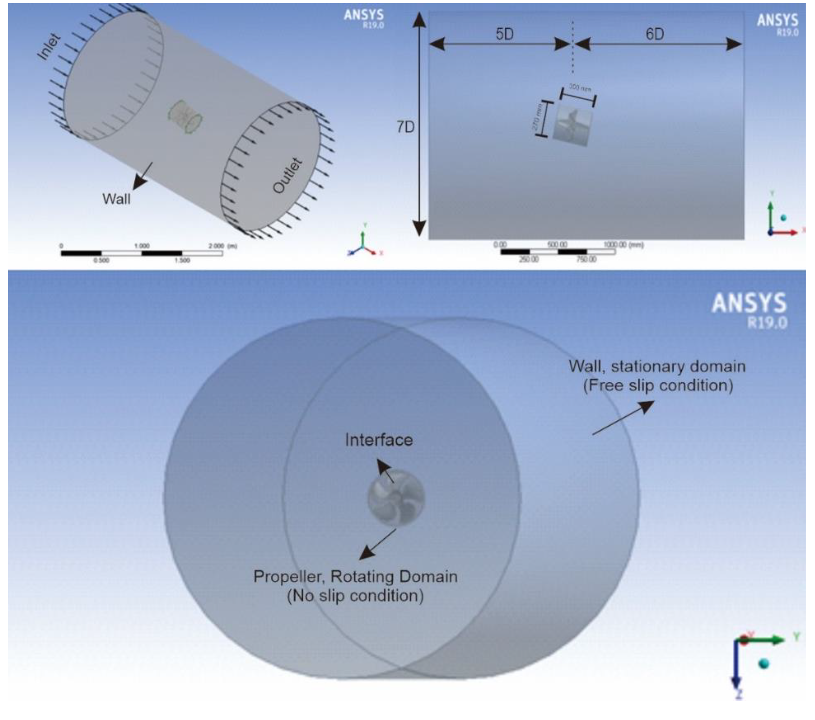
For the simulation under consideration, the computational domain was a cylinder, as shown in Figure 3. The VP1304 propeller has a diameter, D, of 250 mm. The rotating domain had a width and length of 270 mm and 300 mm, respectively. The inlet boundary was placed at a distance of 5D and the outlet was placed at a distance of 6D from the propeller plane. The fixed domain diameter was extended to 7D overall.

The simulations were carried out in 3D assuming a steady state. The propeller moved forward in a homogeneous uniform flow because of the open water conditions. The propeller rotation was simulated using the multiple reference frame (MRF) approach, where the rotational speed was always constant at $n=20 \mathrm{rps}$. This method divides the domain into two pieces of the boundary: Rotating part and a fixed part. The MRF method provides a situation analysis that the rotating domain is relative to other domains, whereas the generalized grid interface (GGI) method provides an approximation to a continuous surface [11]. To obtain the value of advance coefficient $J$ and cavitation number ${\sigma }_n$, the single rotational speed of water was applied. The inlet velocity value was calculated by the advance coefficient $J$. On the inlet, the boundary of turbulent intensity was set at 1%. The pressure outlet for each run was calculated based on the equation of cavitation number ${\sigma }_n$. For all simulations, we assumed that the pressure outlet was $P_{\mathit{Out}}=P_{\mathit{Ref}}$ with a static pressure option. On the outer boundary, the free slip boundary condition was applied, while the propeller or solid surface of the domain was set with a no-slip boundary condition. On the rotating domain, the domain motion was set to rotate with angular velocity. Besides the fixed domain, stationary motion was applied. To influence the transition turbulent flow, first we used SST with automatic wall treatment. In the next step, we applied the standard k-ε for the fully turbulent model with a scalable wall function. The Rayleigh–Plesset equation was involved in describing the growth of cavitation bubbles. Further setup parameters are presented in

Table 3. Numerical setup.

Parameter	Type	Setting
Inlet domain	Normal speed	$\mathrm{Case} 1, u=5.095 \mathsf{m}/\mathsf{s}$ $\mathrm{Case} 2, u=6.345 \mathsf{m}/\mathsf{s}$ $\mathrm{Case} 3, u=7.040 \mathsf{m}/\mathsf{s}$
Inlet heat transfer	Static temperature	$T (\text{°}\mathsf{C})$
Turbulent intensity	Low intensity	$1\%$
Outlet pressure	Static pressure	$P_{\mathit{out}}{=P}_{\mathit{ref}}$
Fluid definition	Volume fraction	Water (1) and vapor (0)
Rotating domain	Angular velocity	20 rps
Multiphase	Mixture	Homogeneous
Heat transfer	Homogenous	Total energy
Turbulent	Shear stress transport	Automatic wall function
Mass transfer	Cavitation	Rayleigh–Plesset
Nucleation	Mean diameter	2 × 10−6
Saturation vapor	Pressure	$P_v$

.

6. Meshing

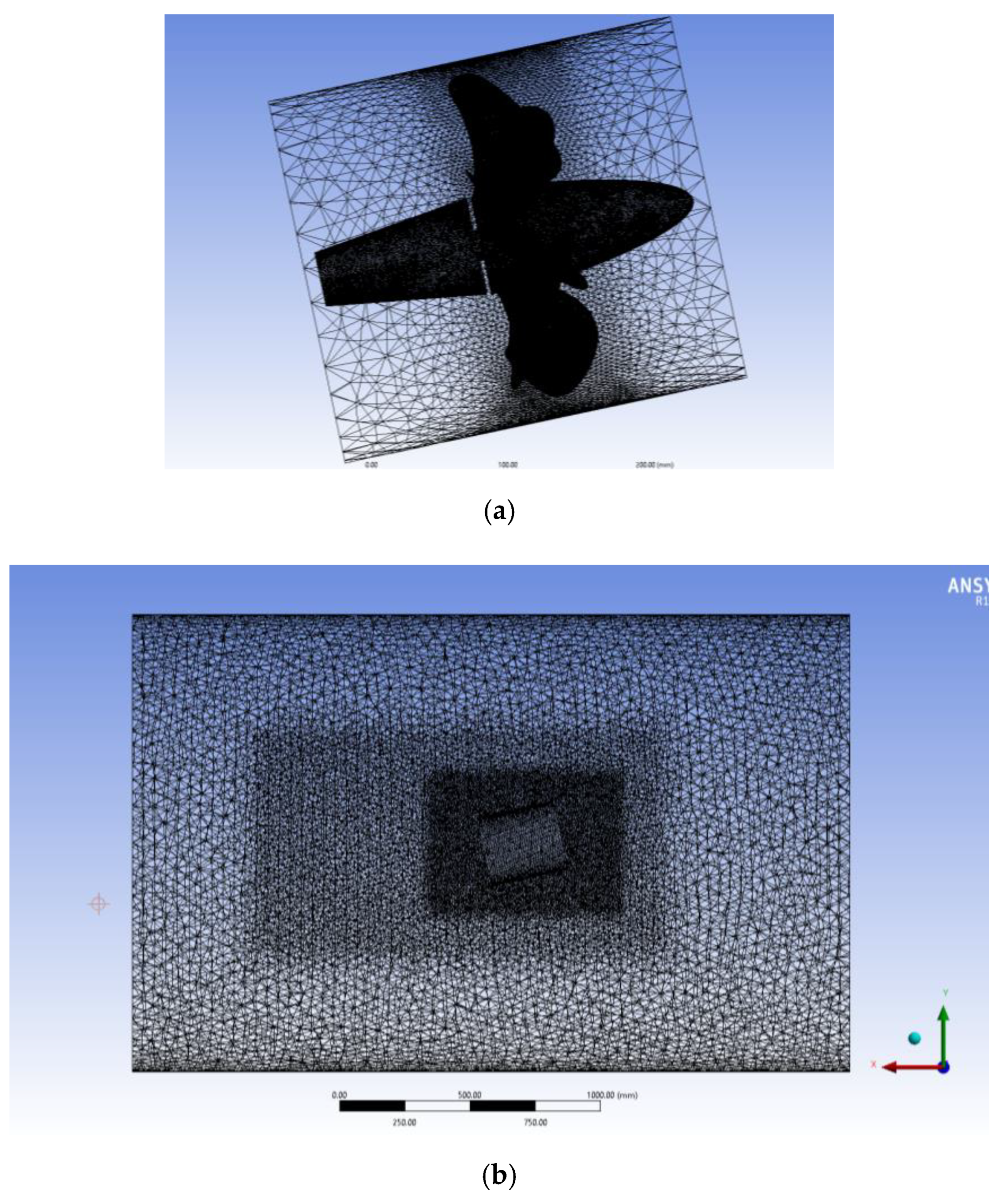
The preferred type of meshing for the propeller is with an unstructured grid and hybrid mesh, which gives high accuracy. In this study, rotating and fixed domain parts were separated. The mesh was generated using the solver mesh of CFX (see Figure 4). The domain initialization for rotating was set with an automatic method, and the fixed domain was established as the tetrahedron method. For the interface of rotating and fixed, CFX solver is capable of joining the meshing approach using a generalized grid interface (GGI). To minimize the number of mesh elements and increase the mesh density, we applied the mesh sizing with the body of influence selection, to approach more accuracy for the critical section. Then, to obtain the viscous effect as the turbulent boundary layer, we placed 11 layers with inflation on the propeller surface. All simulation meshes had the same value of $y^{+}$ of approximately 10 for all propeller surfaces. After convergence, there were 7,301,426 elements and 2,275,988 nodes for the element mesh rotating domain and 2,452,774 elements and 417,994 nodes for the fixed domain. The $y^{+}$ value can be defined with the following equation [29]:

$$y^{+}=\sqrt{\frac{\frac{{\tau }_w}{{\rho }_l} y}{\nu }}$$

(21)

where ${\tau }_w$ is the shear stress at the wall, $\nu$ is the kinematic viscosity of fluid, ${\rho }_l$ is the water density, and $y$ is the normal distance from the wall.

7. Solution and Solver Setting

The CFD software used was Ansys CFX, which provides solutions for three-dimensional viscous cases. The cavitation simulation on the propeller was carried out with the assumption of steady conditions. The advection scheme “upwind” was applied to the transport equation with turbulent numerical high resolution. The dynamic control model was set with velocity-pressure coupling and multi-phase control.

8. Verification and Validation

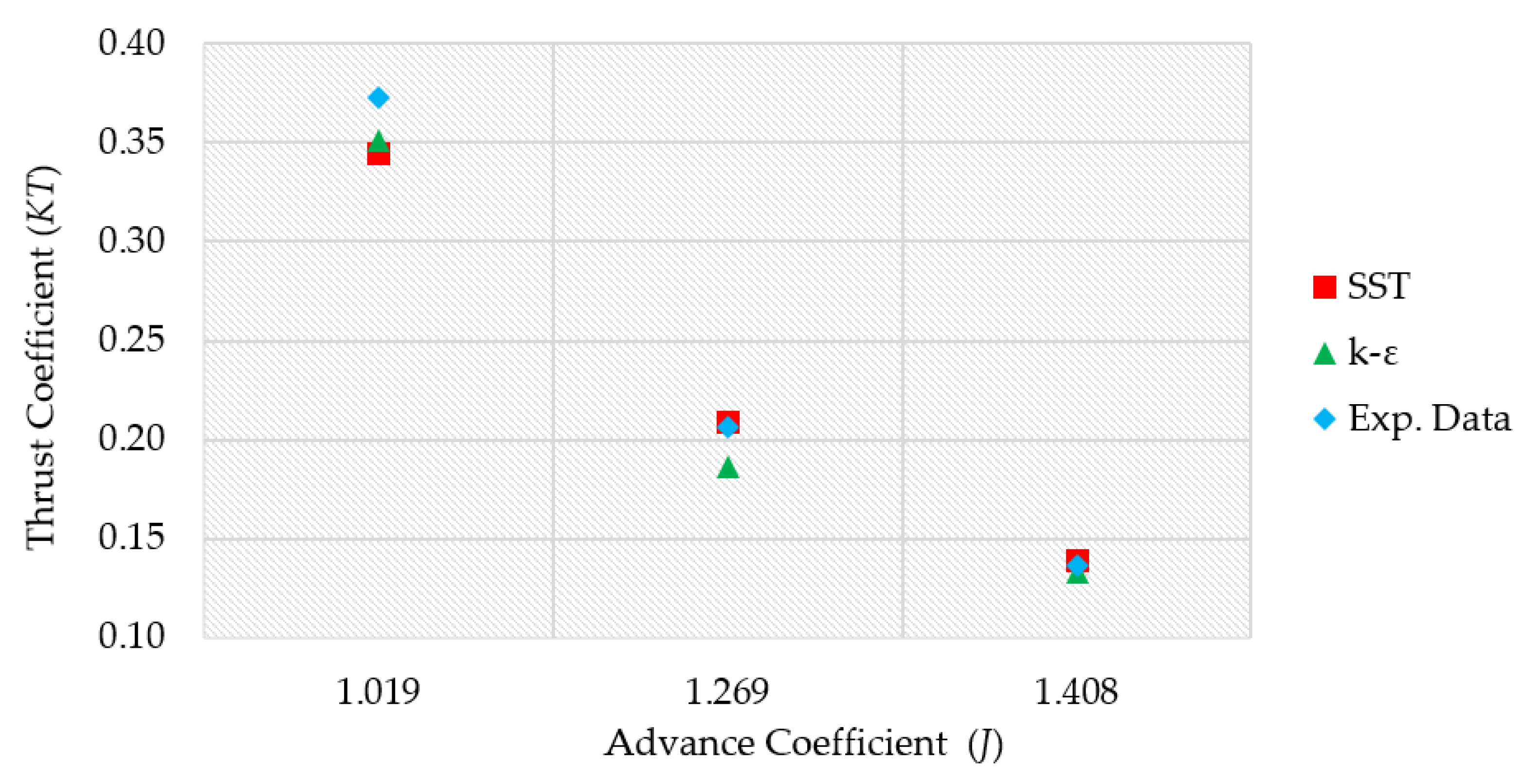
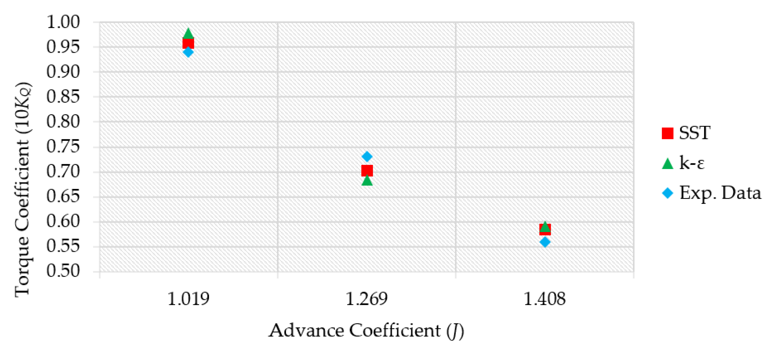
To evaluate the effects of fluid properties and temperature on the cavitation process, we validated the numerical simulation method for cavitation flow behavior. Subsequently, we compared the results of propeller performance at every given operational condition: $(J=1.019, {\sigma }_n=2.024)$, $(J=1.269, {\sigma }_n=1.424), \mathrm{and} (J=1.408, {\sigma }_n=2.000)$. In this section, thrust and torque were obtained from CFX results based on turbulent model k-ε and SST. Afterward, both nondimensional coefficients of performance ($K_T{ \mathrm{and} K}_Q)$ were calculated in every case. The simulation was stopped when the convergence was almost steady and the residual target was reached. The results of the simulation are shown in

Table 4. Numerical results at existing temperature (23.7 °C).

$\mathit{J}$	${\mathit{\sigma }}_{\mathit{n}}$	Experiment		Simulation				Relative Error (%)
		${\mathit{K}}_{\mathit{T}}$	${\mathit{K}}_{\mathit{Q}}$	${\mathit{K}}_{\mathit{T}}$		${\mathit{K}}_{\mathit{Q}}$		${\mathit{K}}_{\mathit{T}}$		${\mathit{K}}_{\mathit{Q}}$
				k–ε	$\mathbf{S}\mathbf{S}\mathbf{T}$	k–ε	$\mathbf{S}\mathbf{S}\mathbf{T}$	k–ε	$\mathbf{S}\mathbf{S}\mathbf{T}$	k–ε	$\mathbf{S}\mathbf{S}\mathbf{T}$
1.019	2.024	0.373	0.123	0.351	0.345	0.098	0.096	−5.8	−7.4	4.2	1.9
1.269	1.424	0.206	0.073	0.186	0.216	0.068	0.071	−9.8	1.2	−6.3	−3.8
1.408	2.000	0.136	0.056	0.133	0.139	0.059	0.058	−2.5	2.3	5.6	4.2

. The validation stage starts with conducting a mesh dependency study to get optimal meshing.

Table 5. Mesh dependency study.

Mesh	Rotating	Fixed	${\mathit{K}}_{\mathit{T}}$	Error
A	4,754,160	1,159,145	0.129	−5.27%
B	7,301,426	2,452,774	0.139	2.32%
C	8,476,318	3,780,050	0.141	3.22%

shows the meshing details based on the number of elements in the rotating and fixed domains. The optimal meshing value was determined based on consideration of simulation time and the accuracy of the data error. The more mesh elements there are, the longer running time is needed. $K_T$ value was calculated based on case 3 at an existing temperature of 23.7 °C. The error value was calculated from the simulation results compared with the experimental data. The experimental data were recorded in the cavitation tunnel of SVA (Potsdam Model Basin) [14].

Based on the data shown in the tables, there are differences in the results of simulation data in experiments with variable errors, assuming steady state and heat transfer during the process were set with total energy. Comparisons revealed that the predicted cavitation at the three operating conditions by both turbulence models was in good agreement with the corresponding data. The agreement between predicted propeller based on both models and experiments was good for the $K_T{ \mathrm{and} K}_Q$ coefficients. There was a difference in the relative error value between turbulent k-ε and SST: k-ε gave a smaller value in thrust and relative error at a higher advance coefficient, while SST had more variable results. In general, based on the simulations that were carried out, we could conclude that the turbulent SST model was better for modeling cavitation than the turbulent k-ε model. For this reason, the simulation in the second stage used entirely turbulent SST models. Figure 5 and Figure 6 present a comparison chart of $K_T \mathrm{and} 10K_Q$ values.

9. Observation Results

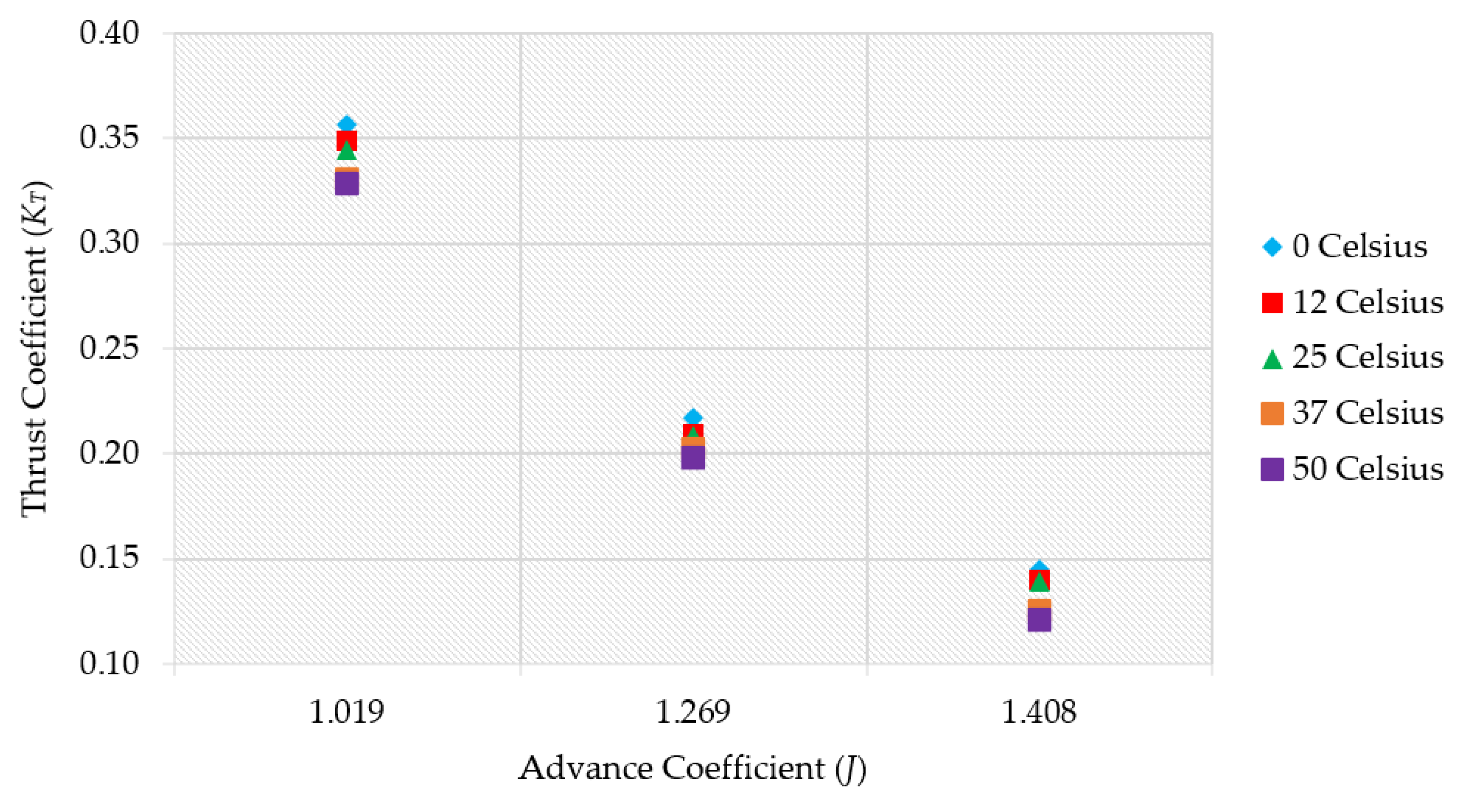
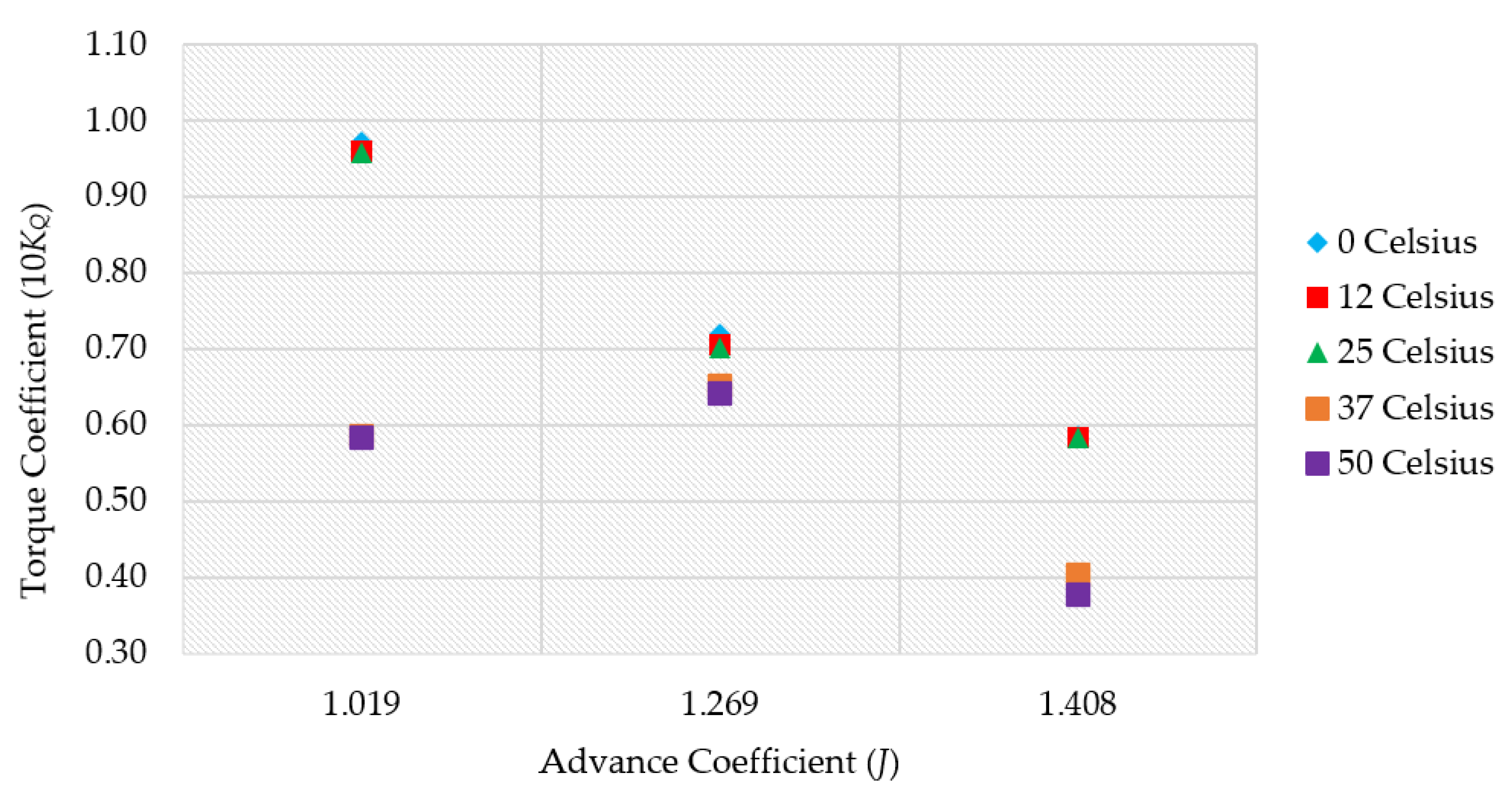
This section shows the results of the simulation.

Table 6. Comparison of propeller performance for case 1 $(J=1.019, {\sigma }_n=2.024)$.

Temperature (°C)	${\mathit{K}}_{\mathit{T}}$	Change in ${\mathit{K}}_{\mathit{T}} (\%)$	$\mathit{10}{{\mathit{K}}_{\mathit{Q}}}_{ }$	$\mathbf{Change} \mathbf{in}$${\mathit{K}}_{\mathit{Q}} (\%)$
Existing Temperature (23.7)	0.345	-	0.958	-
0	0.356	3.378%	0.973	1.470%
12	0.349	1.166%	0.960	0.194%
25	0.345	−0.081%	0.958	−0.063%
37	0.331	−4.100%	0.586	−38.874%
50	0.329	−4.687%	0.585	−38.970%

,

Table 7. Comparison of propeller performance for case 2 $(J=1.269, {\sigma }_n=1.424)$.

Temperature (°C)	${{\mathit{K}}_{\mathit{T}}}_{ }$	Change in ${\mathit{K}}_{\mathit{T}} (\%)$	$\mathit{10}{\mathit{K}}_{\mathit{Q}}$	$\mathbf{Change} \mathbf{in}$${\mathit{K}}_{\mathit{Q}} (\%)$
Existing temperature (23.7)	0.209	–	0.702	–
0	0.217	4.154%	0.721	2.854%
12	0.210	0.475%	0.707	0.822%
25	0.209	−0.024%	0.702	0.084%
37	0.202	−3.111%	0.652	−7.039%
50	0.199	−4.874%	0.642	−8.400%

and

Table 8. Comparison of propeller performance for case 3 $(J=1.408, {\sigma }_n=2.000)$.

Temperature (°C)	${\mathit{K}}_{\mathit{T}}$	Change in ${\mathit{K}}_{\mathit{T}} (\%)$	$\mathit{10}{{\mathit{K}}_{\mathit{Q}}}_{ }$	$\mathbf{Change} \mathbf{in}$${\mathit{K}}_{\mathit{Q}} (\%)$
Existing temperature (23.7)	0.139	–	0.584	–
0	0.145	4.041%	0.585	0.207%
12	0.140	0.737%	0.584	−0.076%
25	0.139	0.029%	0.584	0.038%
37	0.125	−10.299%	0.404	−30.850%
50	0.121	−12.838%	0.378	−35.339%

present the propeller performance parameter data under cavitation conditions. The decreased and increased values of the torque and thrust coefficients were compared with the value in the original case calculation, which was 23.7 °C. A comparison of the performance parameters $K_T$ and $K_Q$ is displayed graphically in Figure 7 and Figure 8. Based on the data in Figure 7 and Figure 8, it is known that at a low temperature of 0 °C, the values of the torque and thrust coefficients were almost the same as in normal temperature conditions; this happened in all cases (case 1–3). The same occurred at 12 °C. The trend of increasing cavitation value was characterized by decreased propeller performance with increasing temperature. The difference in ambient temperature greatly influenced the propeller performance under cavitation conditions.

The results were consistent with experiments conducted by Alarabi [10], who observed the effect of water temperature on centrifugal pumps under cavitation conditions. The experimental results showed that the decrease in the pump head was proportional to the increase in temperature. Dular et al. [32] conducted an experiment comparing cavitation in liquid nitrogen and water with variations in temperature from 20 to 90 °C. Tests showed that the rate of erosion was proportional to the increase in water temperature. The study also revealed that the most significant cavitation occurred at temperatures from 50 to 60 °C. Other research by Plesset, in the form of cavitation experiments on transducers with variations in water temperature from 0 to 90 °C, showed that the largest cavitation causing weight loss occurred at temperatures from 40 to 50 °C [33].

Figure 7 and Figure 8 show comparison graphs of the torque coefficient values. At 37 °C and 50 °C, torque drop occurred in cases 1 and 3, with values dropping significantly compared to normal temperature (25 °C). It is known that the cavitation number influenced the reference pressure, which was close to the water vapor pressure. If the cavitation number is high, the formation of cavitation bubbles becomes very aggressive. This hypothesis was based on research in previous studies stating that $P_v,{ C}_{p, l}, L,{ \mathrm{and} \rho }_v$ play important roles as the primary physical properties that cause cavitation [29]. If cavitation is defined as a decrease in environmental underwater vapor pressure, then the ratio between water vapor pressure and reference pressure becomes inversely proportional. The smaller the ratio, the more aggressive is the inception of the cavitation bubble.

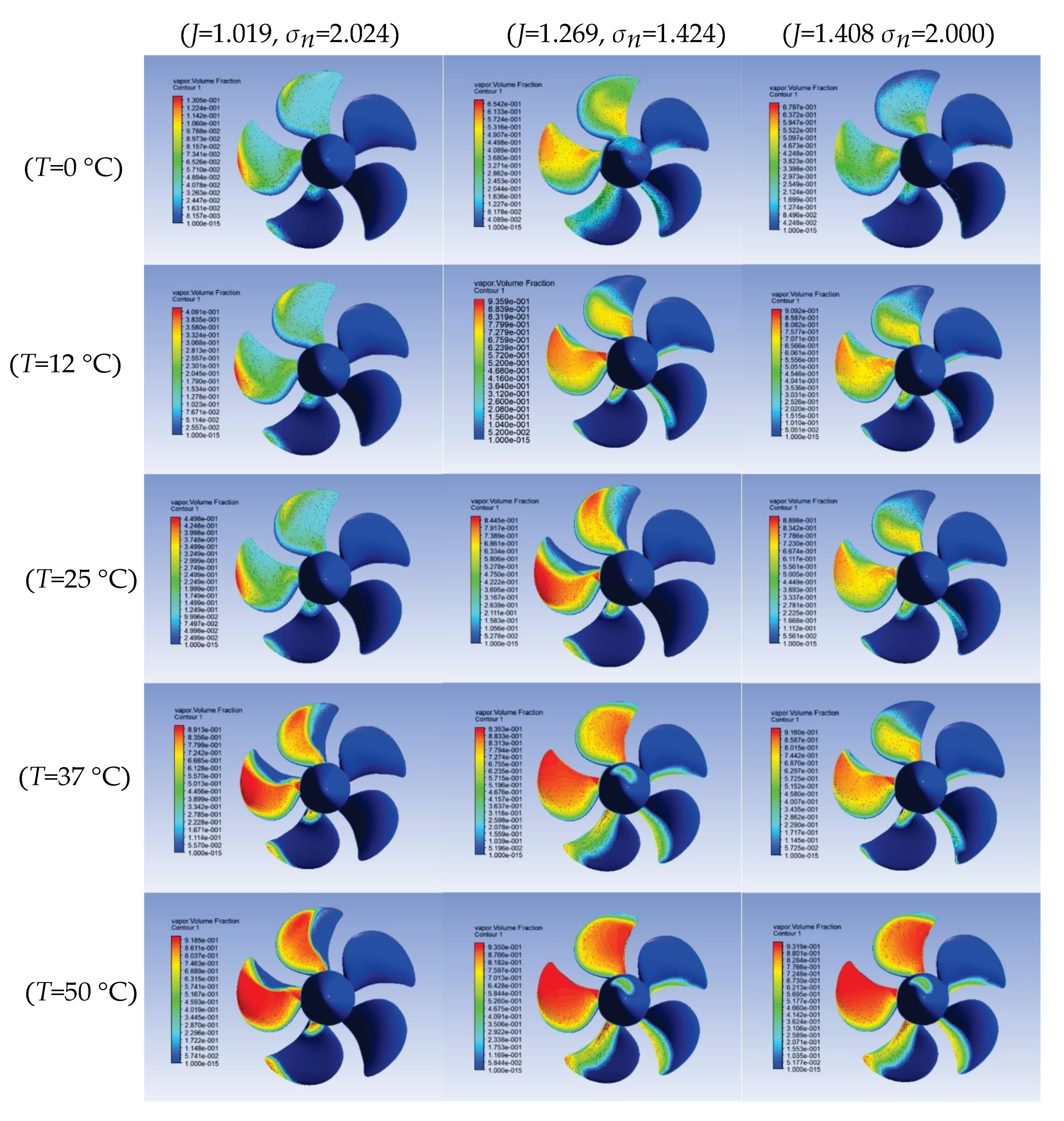
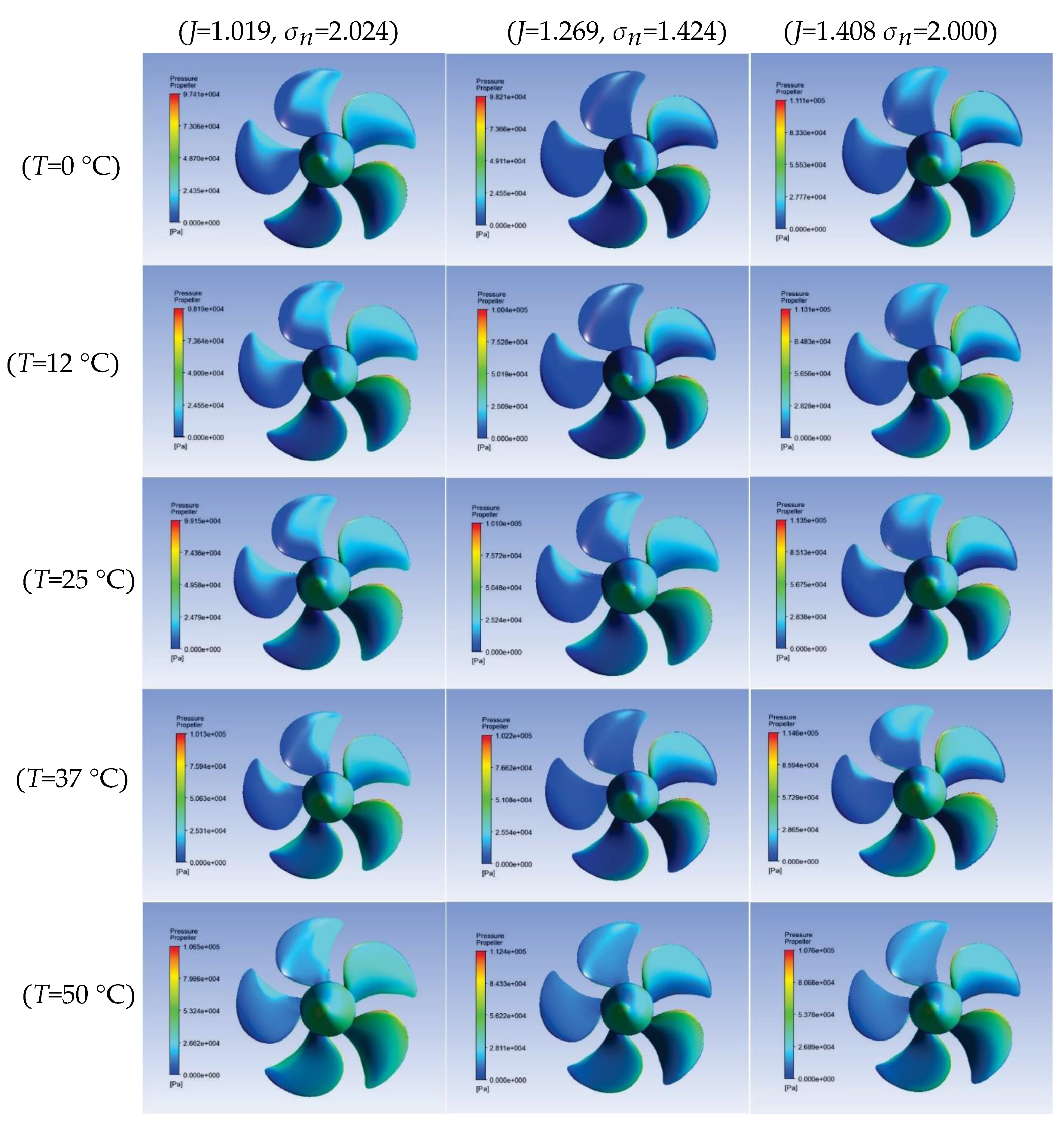
Figure 9 displays the pattern of the vapor volume fraction at a ratio of 0.4. The red area indicates the low pressure at which cavitation bubbles are formed. It can be observed that at higher temperatures, the lower pressure contours of the propeller increase. Vapor density has an important role in cavitation with variable temperature. Water viscosity slightly affects the change in Reynolds number, but it significantly influences the temperature distribution [33]. Figure 9 presents the pressure contour of the propeller suction side. Pressure on the suction side has a relationship with cavitation inception. According to the definition of cavitation, cavitation bubbles will be created in areas where the local pressure is lower than the saturated pressure of water. In Figure 10, blue indicates low pressure areas. In Figure 9, red indicates areas with a high vapor fraction.

10. Conclusions

This paper presented complete and detailed CFD procedures for three-dimensional propeller simulation under cavitation conditions. Then, propeller performance characteristics, propeller cavitation patterns, and comparisons of fluid conditions with different temperatures were presented based on simulations. Fully turbulent k-ε and shear stress models were applied for standard cases to validate the simulation data. Investigations that were carried out on a PPTC1 VP1304 propeller with Ansys had good agreement. The formulation of multi-phase problems using the RANS method with the multiple reference frame (MRF) approach was applied to model the cavitation phenomenon.

The prediction of cavitation in different fluid conditions with the RANS method provided reasonably good agreement. The cavitation model equation with the Rayleigh–Plesset equation provided an initial estimate of the effect of environmental temperature, even though it had a deficiency in data accuracy. A homogeneous model for multi-phase flow and heat transfer was applied to the simulation method.

Transport SST analysis of cavitation erosion at ambient temperature and water fluid properties under three cavitation conditions yielded the following conclusions:

• Cavitation improved equally with increasing temperature, whereas at low temperatures, cavitation inhibited the inception of cavitation bubbles.
• The water vapor pressure ($P_v)$, vapor density $({\rho }_v)$, latent heat (L), and surface tension ($\sigma$) of the liquid played important roles in the rate of cavitation formation based on the different physical properties of water.
• With an increase in temperature, cavitation in case 3 was the most aggressive.
• Cavitation modeling with the Rayleigh–Plesset equation can provide a general description of the effects of different physical properties of water.

Simplifying the simulation method assuming the system was at thermodynamic equilibrium can explain the impact of various physical properties of water with temperature variations, along with the steady state and incompressible simulation approach. Moreover, the results require further verification of different calculations for observed propeller cavitation. An assessment of the generality of our observations in both wetted and cavitating flow is needed. The results of our simulations conform to the theory. However, several assumptions were made to simplify the phenomenon under study. With more accurate data closer to the actual phenomenon, further study of cavitation could be carried out.

Based on these studies, it is believed that this research could be developed as a topic for future work. One aspect that could be followed up is to conduct numerical studies by compressible cavitation modeling with mass transfer not occurring instantly. An unsteady simulation should be performed to approach the real phenomenon. A possible improvement could be to no longer assume instantaneous thermodynamic equilibrium, but allow for a certain “relaxation time” to transfer from non-equilibrium to equilibrium. This would limit the mass transfer between phases and should reduce the need for advanced mathematics to stabilize the solution. Both of these recommendations could lead to improved performance and more stable numerical results when applying the current model and solver to future test cases involving different fluids and temperatures.

References

- Prabowo, A.R.; Putranto, T.; Sohn, J.M. Simulation of the Behavior of a Ship Hull under Grounding: Effect of Applied Element Size on Structural Crashworthiness. J. Mar. Sci. Eng. 2019, 7, 270. [Google Scholar] [CrossRef] [Green Version]
- Bae, D.M.; Prabowo, A.R.; Cao, B.; Sohn, J.M.; Zakki, A.F.; Wang, Q. Numerical Simulation for the Collision between Side Structure and Level Ice in Event of Side Impact Scenario. Lat. Am. J. Solids Struct. 2016, 13, 2691–2704. [Google Scholar] [CrossRef] [Green Version]
- Prabowo, A.R.; Bae, D.M.; Sohn, J.M. Comparing Structural Casualties of the Ro-Ro Vessel Using Straight and Oblique Collision Incidents on the Car Deck. J. Mar. Sci. Eng. 2019, 7, 183. [Google Scholar] [CrossRef] [Green Version]
- Prabowo, A.R.; Bahatmaka, A.; Cho, J.H.; Sohn, J.M.; Bae, D.M.; Samuel, S.; Cao, B. Analysis of Structural Crashworthiness on a Non-Ice Class Tanker during Stranding Accounting for the Sailing Routes. Marit. Transp. Harvest. Sea Resour. 2016, 1, 645–654. [Google Scholar]
- Saleh, B.; Abouel-Kasem, A.; El-Deen, A.E.; Ahmed, S.M. Investigation of Temperature Effects on Cavitation Erosion Behavior Based on Analysis of Erosion Particles. J. Tribol. 2010, 132. [Google Scholar] [CrossRef]
- Morgut, M.; Nobile, E. Numerical Predictions of Cavitating Flow around Model Scale Propellers by CFD and Advance Model Calibration. Int. J. Rotating Mach. 2012, 2012. [Google Scholar] [CrossRef]
- Morgut, M.; Nobile, E. Numerical Predictions of the Cavitating and Non-Cavitating Flow around the Model Scale Propeller PPTC. In Proceedings of the Workshop on Cavitation and Propeller Performance, the 2nd International Symposium on Marine Propulsors (SMP’11), Hamburg, Germany, 15–17 June 2011. [Google Scholar]
- Cooper, J.R.; Dooley, R.B. Revised Release on the IAPWS Industrial Formulation 1997 for the Thermodynamic Properties of Water and Steam; The International Association for the Properties of Water and Steam (IAPWS): Lucerne, Switzerland, 2007. [Google Scholar]
- Spraker, W.A. The Effects of Fluid Properties on Cavitation in Centrifugal Pumps. J. Eng. Gas Turbines Power 1965, 87, 309–318. [Google Scholar] [CrossRef]
- Alarabi, A. Effect of Water Temperature on Centrifugal Pumps Performance under Cavitating and Non-Cavitating Conditions. In Proceedings of the 8th Internal Conference on Sustainable Energy Technologies, Seoul, Korea, 24–27 August 2008; pp. 24–27. [Google Scholar]
- Hosien, M.A.; Selim, S.M. Experimental and Theoretical Investigation on the Effect of Pumped Water Temperature on Cavitation Breakdown in Centrifugal Pumps. J. Appl. Fluid Mech. 2017, 10, 1079–1089. [Google Scholar] [CrossRef]
- Meijn, G.J. Physical Modeling of Cavitation Using an Enthalpy Based Model. In Faculty of Mechanical, Maritime and Material Engineering; Delft University of Technology: Delft, The Netherlands, 2015. [Google Scholar]
- Chivers, T.C. Temperature Effects on Cavitation in a Centrifugal Pump. Theory and Experiment. Proc. Inst. Mech. Eng. 1969, 184, 37–47. [Google Scholar] [CrossRef]
- Lubke, L. Potsdam Propeller Test Case (PPTC) Cavitation in Oblique Flow Case 2. Available online: https://www.sva-potsdam.de/wp-content/uploads/2016/03/3_PPTC-CAV-smp15.pdf (accessed on 1 June 2020).
- Kunz, R.F.; Boger, D.A.; Stinebring, D.R.; Chyczewski, T.S.; Gibeling, H.J.; Venkateswaran, S.; Govindan, T.R. A Preconditioned Navier-Stokes Method for Two-Phase Flows with Application to Cavitation Prediction. In Proceedings of the 14th Computational Fluid Dynamics Conference, Norfolk, VA, USA, 1–5 November 1999; Volume 29, pp. 676–688. [Google Scholar] [CrossRef]
- Salvatore, F.; Greco, L.; Calcagni, D. Computational Analysis of Marine Propeller Performance and Cavitation by Using an Inviscid-Flow BEM Model. In Proceedings of the Second International Symposium on Marine Propulsors (SMP2011), Hamburg, Germany, 15–17 June 2011; p. 8. [Google Scholar]
- Zwart, P.J.; Gerber, A.G.; Belamri, T. A Two-Phase Flow Model for Predicting Cavitation Dynamics. In Proceedings of the Fifth International Conference on Multiphase Flow, Yokohama, Japan, 30 May–4 June 2004; p. 152. [Google Scholar]
- Singhal, A.K.; Athavale, M.M.; Li, H.; Jiang, Y. Mathematical Basis and Validation of the Full Cavitation Model. J. Fluids Eng. Trans. ASME 2002, 124, 617–624. [Google Scholar] [CrossRef]
- Brennen, C.E. Cavitation and Bubble Dynamics; Oxford University Press: Oxford, UK, 1995; ISBN 0-19-509409-3. [Google Scholar]
- Lungu, A. A DES-SST Based Assessment of Hydrodynamic Performances of the Wetted and Cavitating PPTC Propeller. J. Mar. Sci. Eng. 2020, 8, 297. [Google Scholar] [CrossRef] [Green Version]
- Regener, P.B.; Mirsadraee, Y.; Andersen, P. Nominal vs. Effective Wake Fields and Their Influence on Propeller Cavitation Performance. J. Mar. Sci. Eng. 2018, 6, 34. [Google Scholar] [CrossRef] [Green Version]
- Rodio, M.G.; De Giorgi, M.G.; Ficarella, A. Influence of Convective Heat Transfer Modeling on the Estimation of Thermal Effects in Cryogenic Cavitating Flows. Int. J. Heat Mass Transf. 2012, 55, 6538–6554. [Google Scholar] [CrossRef]
- Franc, J.P.; Pellone, C. Analysis of Thermal Effects in a Cavitating Inducer Using Rayleigh Equation. J. Fluids Eng. Trans. ASME 2007, 129, 974–983. [Google Scholar] [CrossRef]
- Viitanen, V.; Siikonen, T.; Sánchez-Caja, A. Cavitation on Model-and Full-Scale Marine Propellers: Steady and Transient Viscous Flow Simulations at Different Reynolds Numbers. J. Mar. Sci. Eng. 2020, 8, 141. [Google Scholar] [CrossRef] [Green Version]
- Pereira, F.A.; Di Felice, F.; Salvatore, F. Propeller Cavitation in Non-Uniform Flow and Correlation with the near Pressure Field. J. Mar. Sci. Eng. 2016, 4, 70. [Google Scholar] [CrossRef] [Green Version]
- Sharqawy, M.H.; Lienhard, V.J.H.; Zubair, S.M. Erratum to Thermophysical Properties of Seawater: A Review of Existing Correlations and Data. Desalin. Water Treat. 2011, 29, 355. [Google Scholar] [CrossRef]
- Lungu, A. Scale Effects on a Tip Rake Propeller Working in Open Water. J. Mar. Sci. Eng. 2019, 7, 404. [Google Scholar] [CrossRef] [Green Version]
- ASIMPTOTE Software. Available online: http://www.asimptote.nl/software/fluidprop/ (accessed on 20 May 2020).
- Helal, M.M.; Ahmed, T.M.; Banawan, A.A.; Kotb, M.A. Numerical Prediction of Sheet Cavitation on Marine Propellers Using CFD Simulation with Transition-Sensitive Turbulence Model. Alexandria Eng. J. 2018, 57, 3805–3815. [Google Scholar] [CrossRef]
- ANSYS CFX-Solver Theory Guide; ANSYS Inc.: Canonsburg, PA, USA, 2009.
- Chen, T.R.; Wang, G.Y.; Huang, B.; Li, D.Q.; Ma, X.J.; Li, X.L. Effects of Physical Properties on Thermo-Fluids Cavitating Flows. J. Phys. Conf. Ser. 2015, 656. [Google Scholar] [CrossRef]
- Dular, M.; Petkovšek, M. Cavitation Erosion in Liquid Nitrogen. Wear 2018, 400, 111–118. [Google Scholar] [CrossRef]
- Plesset, M.S. Temperature Effects in Cavitation Damage. J. Fluids Eng. Trans. ASME 1972, 94, 559–563. [Google Scholar] [CrossRef]
Figure 1.
(a) Density, (b) dynamic viscosity, (c) kinematic viscosity, and (d) vapor pressure of freshwater and seawater [8].
Figure 2.
The 3D pictures of Potsdam Propeller Test Case (PPTC1) model VP1304.
Figure 3.
Design of computational domain.
Figure 4.
(a) Mesh for the rotating domain, (b) mesh for the fixed domain.
Figure 5.
Numerical results of thrust coefficient .
Figure 6.
Numerical results of torque coefficient .
Figure 7.
Numerical/experimental results of thrust coefficient .
Figure 8.
Numerical/experimental results of torque coefficient .
Figure 9.
Comparison of cavitation pattern of the suction side. Results were obtained for the same condition and vapor volume fraction of 0.4.
Figure 10.
Comparison of pressure contour on the suction side. Results were obtained for the same conditions as in Figure 9.