Development of a Fuel Consumption Prediction Model Based on Machine Learning Using Ship In-Service Data

Abstract

As interest in eco-friendly ships increases, methods for status monitoring and forecasting using in-service data from ships are being developed. Models for predicting the energy efficiency of a ship in real time need to effectively process the operational data and be optimized for such an application. This paper presents models that can predict fuel consumption using in-service data collected from a 13,000 TEU class container ship, along with statistical and domain-knowledge methods to select the proper input variables for the models. These methods prevent overfitting and multicollinearity while providing practical applicability. To implement the prediction model, either an artificial neural network (ANN) or multiple linear regression (MLR) were applied, where the ANN-based models showed the best prediction accuracy for both variable selection methods. The goodness of fit of the models based on ANN ranged from $0.9709$ to $0.9936$. Furthermore, sensitivity analysis of the draught under normal operating conditions indicated an optimal draught of 14.79 m, which was very close to the design draught of the target ship, and provides the optimal fuel consumption efficiency. These models could provide valuable information for ship operators to support decision making to maintain efficient operating conditions.

1. Introduction

The environmental pollution resulting from increased consumption of fossil fuels has become a target of the international organizations attempting to regulate greenhouse gas emissions. In 2018, members of the International Maritime Organization agreed to an initial strategy to reduce ship emissions to half of the 2008 level by 2050 [1]; regulations such as the Energy Efficiency Design Index, Energy Efficiency Operational Indicator, and Ship Energy Efficiency Management Plan are being applied to reduce emissions from ships [2,3]. Furthermore, carbon taxes and trading schemes for greenhouse gas emission are being discussed and implemented on the market regulation side [4]. Shipping companies are also developing associated procedures [5], and management plans to maintain international competitiveness and reduce emissions by reducing fuel consumption, which accounts for nearly 50–60% of the total operating expenses [6,7,8].

According to the American Bureau of Shipping, there are three main operational measures for managing the energy efficiency of ships, namely management of: the hull and propeller condition, the ship systems, and the navigation performance [9]. During operation of the ship, marine organisms attach to the hull, which increase the weight and frictional resistance of the hull, resulting in a reduction in the propulsion efficiency [10,11]. Periodic polishing and painting of the hull and propeller surface under the water can increase the propulsion efficiency of the vessel by up to 10% [12]. Since each device on-board consumes electricity, ship system management, which involves optimizing the device performance and performing maintenance at regular intervals, can also improve energy efficiency. Among these approaches, setting an optimal speed during navigation, planning routes considering weather and sea conditions, using proper autopilot modes, and optimizing draught and trim conditions are effective and direct management methods that the ship operator can apply to improve the navigational performance [9].

Recent developments in the field of communication technologies, including data collection and storage, have led to a surge in research related to the management of navigation performance using ship operating data. Beşikçi et al. [13] developed a model to predict the fuel efficiency of oil tankers using the noon report data, including vessel speed, draught, trim, cargo quantity, and weather conditions, where artificial neural network (ANN) models showed better performance than multiple linear regression (MLR) ones. Kim et al. [14] attempted to identify the fuel consumption pattern of a container ship by performing Partial Least Squares (PLS) analysis. In this study, external force factors affecting ships are classified by Beaufort’s wind scale and the input parameters of the model which are influential to the fuel consumption were qualitatively selected based on the experience of experts. Coraddu et al. [15] compared the performance of the white-, grey-, and black-box models to predict fuel consumption of the handymax chemical tanker, and used them to optimize the trim of the ship. According to the study, for limited data, the grey-box model that combines physical relationships and operating data was the most efficient. Wang et al. [16] developed a fuel consumption prediction model that can be applied to various operating conditions with in-service data collected from 97 container ships. They performed the variable selection for voyage parameters using the least absolute shrinkage and selection operator (LASSO), where LASSO regression models offered better accuracy than those based on ANN, a support vector machine (SVM), and a Gaussian process (GP). Gkerekos et al. [17] performed a review of various data-driven methods to find efficient ways to implement the fuel consumption model. The authors used two ships with different data configurations in their research and concluded that models based on measured data could improve the $R^2$ value of the model by 5–7% compared to the use of data from the noon report. Many other studies have estimated the fuel consumption of ships by applying machine learning techniques to noon reports, automatic identification system data, and on-board measurements, and suggested various solutions for energy optimization [18,19,20,21,22] (see

Table A1. Comparison of previous works with this study.

Study	Ship Type	No. of Ships	Data Period	Data Interval	No. of Inputs	Output	Variable Selection Method	Modeling Method
Besikci et al. (2016) [13]	Oil tanker	233	17 months	1 day	7	FOC	-	ANN, MLR
Kim et al. (2017) [14]	Container	1	30 months	10 min	11	FOC, SFOC	Domain-knowledge	PLSR
Coraddu et al. (2017) [15]	Chemical tanker	1	24 months	15 min	41	Shaft power, Shaft torque, FOC	Statistical method (BFM, RBM, RFM)	White, Grey, Black box
Wang et al. (2018) [16]	Container	97	36 months	-	21	FOC	Statistical method (LASSO)	MLR, SVM, GP, ANN
Yuan and Nian (2018) [56]	Oil tanker	1	18 months	-	7	FOC	-	GP
Jeon et al. (2018) [19]	Bulk carrier	1	abt. 42 days	15 min	7	FOC	-	ANN, MR, SVM
Uyanik et al. (2019) [20]	Commercial vessel	1	abt. 35 days	1 day	5	FOC	-	ANN, MLR
Hu et al. (2019) [21]	Container	1	1 year	15 min	10	FOC	-	GP, ANN
Gkerekos et al. (2019) [17]	Reefer vessel, Bulk carrier	2	30 months, 1 month	1 day, 1 h	12	FOC	Statistical methods	12 Machine learning methods
Farag and Ölçer (2020) [22]	Oil tanker	1	2 voyages	abt. 10 min	11	FOC, BSFC	-	ANN, MLR
This study	Container	1	6 months	1 min	11	Fuel efficiency	Domain-knowledge, Statistical method (LASSO)	ANN, MLR

FOC: Fuel oil consumption, SFOC: Specific fuel oil consumption, BSFC: Brake-specific fuel consumption, BFM: Brute force method, RBM: Regularization based method, RFM: Random forest based method, LASSO: Least absolute shrinkage and selection operator, ANN: Artificial neural network, MLR: Multiple linear regression, SVM: Support vector machine, PLSR: Partial least square regression, GP: Gaussian process.

).

In summary, the existing gaps in the literature are as follows. Although many studies have been performed, differences between the practical requirements of navigational management and the predictions of the fuel consumption models persist as the field continues to rely on the experience of workers at ship sites. The previous studies mainly addressed optimization at the design level of the vessel through water tank experiments or numerical simulations, while improvements in the operational performance were not sufficiently considered from the viewpoint of the ship operator, who is responsible for planning the voyage and/or monitoring the ship operation. That is, the input variables of this model need to consist of factors that can be changed on the vessel by the operator’s action in real-time. On the other hand, when creating an analytical model based on operation data, it is important to pay attention to the variable selection of the model. This is because there are many characteristic variables associated with the ship’s operational performance, some of which are strongly correlated with each other. If these characteristic variables are directly used in a prediction model, inaccurate estimation of regression coefficients and multicollinearity between variables may occur [23,24]. Previous studies have rarely shown solutions to overcome these two perspectives of fuel consumption models.

In this study, we developed two models for predicting the fuel consumption from in-service data collected from a 13,000 TEU (twenty-foot equivalent units) class container ship. To select proper independent variables for implementing the prediction model, a statistical method and a domain-knowledge-based method were used for the first and second approaches, respectively. These methods were used to solve the multicollinearity problem between input variables while selecting statistically significant variables, and to consider the practical input settings used in ship operation. The models were developed based on an ANN or MLR, and their performance was verified by an independent test case. Finally, sensitivity analysis of the draught under normal operating conditions of the target ship was performed to identify the optimal operating draught that maximized the overall energy efficiency, which was compared with the design draught of the ship.

2. Materials and Methods

2.1. Modeling Methods and Algorithms

The procedure used in this study is described below.

(i)

Data pre-processing: This step was used to remove outliers or noise contained in the raw data sets that are inappropriate for data analysis before implementation of the model. Outliers were defined as data points outside of 3 standard deviations from the simple linear regression line between variables such as power-fuel consumption, where such values were compared with the trend of the time-series data to determine the validity of the process. Then, data smoothing with a median filter was performed to obtain the trend of variables such as draught or trim, as these values change continuously due to movement of the ship. Curve fitting in various functional forms was used to consider the nonlinear physical relationships between the independent variables and the dependent variable. Finally, standardization of the data was performed to match the scales of the independent variables.

(ii)

Variable selection: The independent variables of the predictive model that have a significant influence on fuel consumption were selected using both domain-knowledge and statistical methods. To expand the practicability of the model, candidate variables recommended by ship experts for increasing energy efficiency were considered. In addition, the LASSO regularization method was used to overcome problems such as multicollinearity of the model due to the correlation between input variables.

(iii)

Model implementation: This step sought to implement a fuel consumption prediction model using pre-processed data from the previous step. The overall dataset was randomly divided in a ratio of 7:3, with the former set being used to train the model (training data set) and the latter as a performance evaluation of the model (test data set). The variables selected in the previous step (ii) according to the variable selection of domain-knowledge method or statistical method were used as independent variables of the model. MLR and ANN methods were used to implement the model. For ANN models, the appropriate structure was determined by analyzing the accuracy of the model according to the number of hidden layers and nodes.

(iv)

Model validation: The prediction accuracy of the developed models were validated by comparing the test data set (remaining 30% of the data) with the predicted values. In addition, the fuel efficiency of the ship over an independent voyage period data, which never used for training data set or test data set of the model, was predicted and compared. Finally, a sensitivity analysis on the draught of the ship was performed as a case study to evaluate the sensitivity of the fuel efficiency to changes in the input variables over a range of typical operating conditions of the vessel.

2.2. Target Ship and Operational Data

This study was conducted based on data from a 13,000 TEU class container ship with dimensions, as given in

Table 1. Principal dimensions of the target ship.

Ship Particular	Dimension
Total length	abt. 360.0 [m]
Length between perpendiculars	abt. 350.0 [m]
Moulded breadth	abt. 50.0 [m]
Moulded depth	abt. 30.0 [m]
Design draught	abt. 14.5 [m]
Gross tonnage	abt. 141,000.0 [ton]
Displacement	abt. 185,000.0 [ton]

. The main engine system of the vessel was equipped with a two-stroke engine rated 68,640 kW and designed for operation at 102 rpm. It was connected to a fixed-pitch propeller (diameter 8.8 m with 6 blades) with the gearbox between.

The operational data was collected at one-minute intervals from the alarm monitoring and control system (AMS) of the vessel from January to June 2014. During this period, the target ship sailed on the Asia-Europe route as described in

Table 2. Voyage schedule of the target ship.

	Port Rotation
West Bound	Xingang (China)-Kwangyang (South Korea)-Pusan (South Korea)
	-Shanghai (China)-Xiamen (China)-Yantian (China)-Singapore
	-Suez (Egypt)-Algeciras (Spain)-Hamburg (Germany)
East Bound	Hamburg (Germany)-Rotterdam (Netherland)-Lehavre (France)
	-Algeciras (Spain)-Suez (Egypt)-Singapore-Yantian (China)
	-Hongkong (China)-Xingang (China)

, and one round trip voyage was approximately 83 days. The collected raw data consisted of 65%, 17%, and 18%, of sailing, port stays and maneuvering sections near port areas, and missing data, respectively. To investigate the energy efficiency of a ship in service, we used the data only from the sailing periods.

In-service data of the target ship including speed, loading condition, power consumption, and environmental factors were collected, and the variables used in the prediction model are listed in

Table 3. Ship parameters used in the study to predict fuel consumption.

Data Type	Parameter	Unit	Remark
Input	Main engine RPM (RPM)	revolution/min
	Speed over the ground (SOG)	knot
	Speed through water (STW)	knot
	Relative wind speed (RWS)	knot
	Relative wind direction (RWD)	°	Relative angle against ship heading
	Rudder angle (RUD)	°
	Mean draught (DFT)	m	Mean of forward and afterward draught
	Trim (TRM)	m	$(+),(-)$: Trim by the stern, the head
	Displacement (DIS)	ton
	Wetted surface area (WSA)	${\mathrm{m}}^2$
	Difference between STW and SOG (DBS)	knot
Output	Fuel efficiency (FEF)	ton/nautical mile

. The difference between the speed over the ground (SOG) and speed through water (STW) obtained from the vessel was taken as an external force variable to consider the momentary effect of the ocean current. The growth of marine organisms and damage of the hull painting can increase hull roughness, while cleaning and painting of hull and propeller result in the opposite effect. These factors can affect the propulsion performance of the vessel. However, the target vessel of this study is a container ship contracted to serve the Asia–Europe voyage and sailed continuously for 6 months, except for relatively short cargo operation time in the port. Furthermore, there was no record of a vessel cleaning or painting of the hull and propeller during the corresponding period. Therefore, we assumed that the difference in propulsion performance due to the hull roughness change during the data collection period in this study was not significant. The fuel consumption of the ship can be expressed as the sum of the fuel consumed by the main engine, auxiliary engine, boiler, and other components. Only the fuel consumption measured by the accumulated mass flow meter of the main engine was used to determine the energy used to propel the ship. As the main engine power of the ship was directly related to fuel consumption, it was excluded from the candidate parameters for the model.

Many previous studies used fuel consumption per unit hour as their dependent variable, which is a useful indicator of fuel efficiency assuming similar ship operating conditions [17,21,22]. However, direct comparison of fuel consumption per hour may be somewhat inaccurate in different situations, as fuel consumption and the sailing distance depending on their operating conditions, such as the loading condition of the vessel or the sea-state and weather of the navigation area. In particular, as the aim of this study was to develop a fuel consumption model to assist ship operators in the decision-making process, we propose the use of fuel consumption per unit sailing distance as a better dependent variable (Equation (1)), which facilitates the determination of the energy efficiency considering the environmental conditions.

$$Fuelefficiency[ton/nauticalmile]=\frac{Fuelconsumptionperunittime[ton/hour]}{Sailingdistanceperunittime[nauticalmile/hour]}$$

(1)

2.3. Data Pre-Processing

2.3.1. Outlier Detection Based on 3$\sigma$-Rule

The 3$\sigma$-rule is a simple and widespread method for detecting outliers, where about 99.7% of the total data is within three standard deviations of the observed data, and outliers are defined as data points outside this range [25,26]. As shown in Equation (2), if the least-squares residual of observation exceeds three times its standard deviation, it is considered as an outlier, otherwise a normal value.

$$x_i=\left\{\begin{array}{cc}\mathrm{outlier},\hfill & \mathrm{if}|x_i-\mu |>3\sigma .\hfill \\ \mathrm{normal},\hfill & \mathrm{otherwise}.\hfill \end{array}\right.$$

(2)

where $x_i$ represents the i-th observed data point, $\mu$ is the mean of all observed data, and $\sigma$ is the standard deviation.

The outliers of the current data set were identified using the relationship between the power of the main engine and fuel consumption, which was identified by simple linear regression [27]. Under the assumption that the difference between the values predicted by the regression analysis and the observed values are normally distributed, the observed values outside the 3$\sigma$ range were labeled as outliers. Figure 1 shows a scatter plot of the fuel consumption vs. engine power, where the solid line is the linear regression result, and the data points inside and outside the 3$\sigma$ range are indicated by different symbols. One major outlier was sampled (as indicated in Figure 1), and the time-series data for the fuel consumption and engine power at the corresponding point is shown in Figure 2. Given the trends in both curves over time, the engine power at the sampling point was regarded as abnormal. Since the ratio of outliers detected at this stage to the total sample size is relatively small, data sets containing such values were removed from the raw data sets rather than replacing them with other values.

2.3.2. Data Smoothing Using a Median Filter

Since the draught or trim values change continuously due to the movement of the ship through the water, especially in rough weather, it can be difficult to obtain the exact operating conditions of the ship in a specific moment [28,29]. Therefore, when using such values for analysis, due consideration of the collection interval and quality of the data is critical. In this study, the data were collected at one-minute intervals, which are instantaneous data at the time of the acquisition, not the average value for that period. This made it difficult to observe consistent overall trends; hence, a median filter was applied to compensate for this. The median filter replaces the corresponding observation with the median value of a specified window of the data set arranged in ascending or descending order, as shown in Equation (3). It is an effective method for reproducing the overall tendency of the data by removing outliers within a time-series data [30]. Pedersen and Larsen [31] and Perera and Mo [32] used average filters with a 10–15-min window to analyze in-service data. Here, we performed filtering based on a 10 min window. In this study, the heave and pitch motions of the ship could not be accurately measured because of the unavailability of suitable sensors. However, we incorporated the impact on the amplitude of the pitch and heave motions indirectly by applying the median filter on the trim and draught data of one-minute intervals. Figure 3 shows the result of applying the median filter to the average draught and trim, which are the most volatile of the real-time operational data.

Table 4. Results of statistical analysis of the input parameters after applying outlier detection and data smoothing.

Parameter	Mean	Std. Dev	Min	Max	Median	Skewness
RPM	63.45	7.47	50.00	90.00	63.00	0.09
SOG	14.71	2.01	8.00	22.40	14.80	0.05
STW	14.54	1.88	7.40	21.80	14.50	0.10
RWS	19.61	10.15	0.00	72.89	18.86	0.56
RWD	43.07	43.45	0.00	180.00	23.60	1.35
RUD	1.64	2.43	0.00	36.10	0.90	4.03
DFT	14.26	0.94	11.25	15.70	14.60	−1.38
TRM	−0.05	0.58	−2.30	2.15	−0.15	1.07
DIS	163,225.08	13,240.08	123,466.40	184,009.60	167,898.20	−1.35
WSA	14,047.80	292.93	13,108.02	14,514.28	14,151.05	−1.28
DBS	0.17	0.69	−3.50	3.70	0.20	0.05
FEF	0.21	0.05	0.08	0.48	0.20	0.41

shows the results of statistical analysis of the variables after pre-processing by applying outlier detection and data smoothing.

$$\widehat{x}\left(t\right)=median[x\left(t\right),x(t+1),\cdots ,x(t+i)]$$

(3)

where $x\left(t\right)$ is x value at time t, i is the window size, and $\widehat{x}\left(t\right)$ is median of x values from time t to $t+i$.

2.3.3. Variable Transformation Using Curve Fitting

The energy consumption of a ship is closely related to its operating parameters and can be expressed by various physical relationships. Simple linear regression can only accurately describe highly linear relationships between the variables. Therefore, in this study, various functional forms, such as quadratic, cubic, inverse, logarithmic, and exponential, were used in addition to linear fitting to more accurately describe the variables. Figure 4 shows the top four functions with high coefficients of determination ($R^2$) among the different types of curve fittings compared with scatter plots of the fuel efficiency as a function of each ship parameter. Each ship parameter was converted to the appropriate data distribution using the function with the highest coefficient of determination (see

Table 5. Results of curve fitting of input variables.

	RPM	STW	SOG	RWS	RWD	RUD	DFT	TRM	DIS	WSA	DBS
Function	L	C	C	Q	C	C	C	L	C	C	L
$R^2$	0.7955	0.3943	0.5567	0.1503	0.0771	0.0108	0.3218	0.1482	0.3286	0.3690	0.0541

L = Linear, Q = Quadratic, C = Cubic, I = Inverse, G = Logarithmic, E = Exponential.

). However, if the difference between the coefficients of determination of curve fitting functions was not significant, the function with the lower order function was selected to reduce the complexity of the model.

2.3.4. Data Standardization

Since each variable generally uses a different unit system, it is difficult to accurately determine the influence of the independent variable on the dependent variable when estimating the regression coefficient. To prevent this, z-score calculations were performed to standardize the data, as shown in Equation (4). The standardized variable has a mean of 0 and a standard deviation of 1.

$$z_i=\frac{x_i-\mu }{\sigma },\forall i=1,2,...,p$$

(4)

where $x_i$ is the i-th observed value of each variable, $\sigma$ is the standard deviation, $\mu$ is the mean, $z_i$ is the standardized value, and p is the number of observations for each variable. In this study, p corresponds to data acquired every minute for six months.

2.4. Variable Selection

A ship’s sailing plan is established in comprehensive consideration of the port schedules, sea and weather conditions, and safe sailing areas, and relies heavily on the knowledge and experience of the skilled ship operators [33,34]. Several models have been developed to determine the energy efficiency of ships and support the decision-making of ship operators, but they do not provide all of the factors necessary for route planning. Most methods focused on optimizing the ship design, rather than the navigational plan [35]. In addition, when all available data is used to implement the model, as in some previous studies, the high correlation between the variables and the use of unnecessary data can cause problems with multicollinearity and overfitting of the predictive model [23,24], which results in long computational times and high costs [36,37]. To provide a solution for this, we propose two variable-selection methods for implementing the model: domain-knowledge method and statistical method.

2.4.1. Domain-Knowledge Method

If the model is used during pre-sailing planning or during sailing for the purpose of predicting fuel consumption and energy-efficient sailing, the variables that can be adjusted on the actual vessel by the ship operator’s actions or environmental variables that may affect them should be selected as the main input variables. These inputs should be either directly entered by the user or automatically entered from the on-board system. Therefore, the main variables of the model were selected considering the experience of ship operators and the vessel energy efficiency measures published by the American Bureau of Shipping [9]. These guidelines propose operational measures for reducing fuel consumption and greenhouse gas emissions. The main operational factors relevant for reducing fuel consumption are voyage speed optimization, weather routing (considering both energy efficiency and safety), trim/draught optimization, and autopilot optimization.

Operating the ship at optimum speed is a very effective method for increasing the energy efficiency, where the variables in the present data set related to the speed include the main engine RPM, SOG, and STW. The sailing speed of a vessel is generally maintained above the target speed to reach the destination within a defined port schedule. Although ship navigation officers control the main engine RPM to meet the target speed, the RPM may vary depending on the weather or the ship loading conditions, and the final speed controlled by the RPM is required to make navigation decisions. Therefore, the SOG was chosen here as the relevant variable for ship speed optimization.

Weather routing provides weather information around the anticipated route in advance. It has been reported that optimal route support services, which can help ships reach their destinations under various weather and sea conditions, can reduce fuel consumption by up to 3% [38]. The main aim of this study was to create a fuel consumption model with data that can be measured from on-board. From the practical point of view, few vessels are equipped with wave radars except ocean survey ships and special purpose vessels. Most cargo ships acquire 72, 48, or 24 h pre-weather forecast data for safe navigation from paid weather services subscribed by ship owners, or even worse cases, less accurate data is achieved. In contrast, Chapter V of the International Convention for the Safety of Life at Sea (SOLAS), 1974 [39] regulates that all cargo ships with more than 500 tons shall be equipped with equipment available for measuring wind speed and direction, and the real-time measurement onboard is fairly accurate. Although measured wind data cannot fully describe all environmental variables in the navigation area (especially wave characteristics), ocean waves are developed by the local wind which represents a significant portion of the wave characteristics [40,41,42]. Thus, this study included wind data as the main environmental variables in the navigation area. Additionaly, the influence of the external forces due to ocean currents was defined as the DBS.

The energy consumed by the vessel also depends on the loading conditions [43], and adjusting the draught and trim of the vessel with the appropriate amount of ballast water is a simple and inexpensive way to optimize the energy use of the vessel. The hull shape is traditionally designed to have optimal energy efficiency according to specific draught and trim. Even with the same volume displacement, ship resistance varies depending on the draught and the trim, which may affect fuel consumption. In addition, increasing the amount of cargo increases the draught and displacement of the vessel, which increases resistance and fuel consumption. In-service data of the several round-trip voyages can include not only changes in trim and draught due to the consumption of fuel and freshwater but also changes in trim and draught due to different loading conditions for each port-to-port section. In this study, we used such data set to implement the model to reflect the impact of loading conditions on fuel consumption.

The rudder operation used for the course change of a ship creates additional drag [44]. Although resistance due to the steering typically accounts for a small percentage of total hull resistance, minimizing unnecessary rudder usage and rudder angles can reduce total fuel consumption by up to 1% [9]. If the vessel is equipped with an autopilot system, the rudder can automatically be used to maintain a predetermined course, while optimizing the fuel efficiency of the vessel for specific operating conditions. However, according to the analysis of the rudder usage data collected in this study, most of the rudder use was due to continuous control by the auto-pilot system to keep a constant course, and relatively there were not many manual operations by the navigators. Moreover, since rudder angle cannot be determined by the ship navigator before the voyage commences and is not generally used in voyage planning, it was excluded as an input variable for the fuel efficiency prediction model based on domain-knowledge. Six main input variables were selected based on the domain-knowledge of experts, namely SOG, RWS, RWD, DFT, TRM, and DBS.

2.4.2. Statistical Approach Based on LASSO Regularization

LASSO regularization is a method of reducing the regression coefficients of the independent variables that are less dependent on the dependent variable due to the assignment of a tuning parameter to the magnitude of the regression coefficient. Assigning the regression coefficients of insignificant variables as zero allows for variable selection and thus produces models with high analytical power [45]. LASSO regularization adds a term that minimizes the sum of absolute regression coefficients as a constraint and minimizes the sum of the squared residuals normally used in regression analysis, as in Equation (5), i.e., the objective is to find regression coefficients that minimize the sum of the two terms ($\beta$, $\lambda$). As $\lambda$ increases, the degree of regularization increases, and the regression coefficient decreases. When $\lambda$ decreases, the degree of regularization decreases, and when it becomes 0, a general linear regression model is achieved. Figure 5 represents the geometric structure of the LASSO regression, and the coordinate axis shows the estimator of each regression coefficient. The residual sum of squares is defined by an elliptic contour, and the constraint boundary is represented by a square rotated area. The estimated LASSO regression coefficient converges to zero at the point where the contour and the constraint boundary meet, allowing the variable selection.

$${\widehat{\beta }}^{lasso}={argmin}_{\beta }\left\{\sum _{i=1}^n{\left(y_i-{\beta }_0-\sum _{j=1}^p{\beta }_j{x}_{ij}\right)}^2+\lambda \sum _{j=1}^p\left|{\beta }_j\right|\right\}$$

(5)

where p is the number of independent variables, and $\lambda$ is the tuning parameter for controlling the weight of the existing residual sum of squares and additional constraints.

Since LASSO regularization is a statistical method for selecting variables, to investigate the effect of curve fitting, it was applied to the same data before and after variable transformation through curve fitting, as described in Section 2.3.3. Here, 10-fold cross-validation was performed to locate the value that minimizes the mean squared error (MSE), and the one standard error rule was used to select a tuning parameter within the range of one standard error from the point where the minimum MSE occurs by performing cross-validation [26]. The variable selection by LASSO regularization identified 9 variables (RPM, SOG, STW, RWS, RWD, RUD, TRM, WSA, and DBS), while the addition of curve fitting resulted in the selection of 6 variables (RPM, SOG, STW, RWS, RUD, and DBS).

2.5. Model Implementation

The prediction model was implemented using the data processed as described in Section 2.3, with the selected variables listed in Section 2.4. Both MLR and ANN were used to train the data, and a total of 8 cases were developed according to the variable selection methods and modeling algorithms, as described in

Table 6. Comparison of model cases.

Case	Variable Selection Method	Modeling Method
1	Domain-knowledge	Regression
2	Domain-knowledge	Curve fitting + Regression
3	Domain-knowledge	ANN
4	Domain-knowledge	Curve fitting + ANN
5	LASSO regularization	Regression
6	LASSO regularization	Curve fitting + Regression
7	LASSO regularization	ANN
8	LASSO regularization	Curve fitting + ANN

. To compare the performance of curve fitting covered in Section 2.3.3, we applied curve fitting to the input variables of ANN as well as the MLR and included them as comparison cases.

Ship operations can generally be divided into ballast and laden, and training the model by dividing these sections would further enhance the reliability of the model by reflecting the character of each navigation pattern. However, unlike bulk carriers or tankers, container ships typically load and unload containers at multiple ports during one voyage, which made it difficult to classify the trade pattern [43]. In addition, some data sections that were invalid for analysis were removed in the pre-processing procedure, and hence, the amount of valid data varied for each voyage. Therefore, the model was trained without distinction by navigation patterns. In other words, the entire data set was randomly divided with a ratio of 7:3, wherein the former set was used as the training set, and the latter used for evaluating the developed model.

2.5.1. Multiple Linear Regression Model

Regression analysis is used to describe the relationship between independent and dependent variables or to predict the output of new input. The basic model of MLR analysis with k independent variables is expressed by Equation (6). Regression analysis estimates the regression coefficients ${\beta }_0$-${\beta }_k$ corresponding to each independent variable. The least-squares method is used to find the regression coefficients that minimize the residual sum of squares, as given by Equation (7). The parameters selected in Section 2.4 were used as each independent variable in the MLR model, and each input value differed depending on the model cases. For example, in Case 1 and Case 5, the standardized values of each variable were used as input values, and in Case 2 and Case 6, the standardized values after variable transformation through curve fitting were used.

$$y_i={\beta }_0+{\beta }_1{x}_{1i}+{\beta }_2{x}_{2i}+·+{\beta }_k{x}_{ki}+{ϵ}_i$$

(6)

$$\widehat{\beta }={argmin}_{\beta }\sum _{i=1}^n{\left(y_i-{\beta }_0-\sum _{j=1}^p{\beta }_j{x}_{ij}\right)}^2$$

(7)

where $x_{1i}$, $x_{2i}$,…, $x_{ki}$ are the i-th observed values of independent variables, ${\beta }_1$, ${\beta }_2$,…, ${\beta }_k$ are the regression coefficients, ${\beta }_0$ is intercept term, ${ϵ}_i$ is a residual, n is the sample size, p is the number of independent variables, and $y_i$ is i-th observed value of dependent variable.

2.5.2. Artificial Neural Network Model

ANN is a simplified model of the human neural network structure, which sums the products of the input chemical signal coming from the synapse, with the weight of the connection strength of the synapse, and finally the output value is derived via an activation function [46]. A simple ANN is expressed by Equations (8) and (9).

$$v=b+\sum _{i=1}^n{w}_i{x}_i$$

(8)

$$y=f\left(v\right)$$

(9)

where $x_i$ is the ith input, $w_i$ is the ith weight, b is the bias, v is the summed output, f is the activation function, and y is the output.

A multilayer perceptron, composed of three or more layers, has a similar structure to a single-phase perceptron, but has at least one intermediate layer called a hidden layer between the input and output layers to enable learning about nonlinear data [47]. The nonlinear relationship between the input and output is given by various activation functions (e.g., staircase, critical logic, and sigmoid) in the hidden layer. The rectified linear unit (RELU) is a simple and efficient activation function that helps solve the problem of vanishing gradients in neural networks [48,49], as described by Equation (10). The schematic diagram of the multi-perceptron-based fuel efficiency prediction model implemented in this study is shown in Figure 6.

$$f\left(x\right)=max(0,x)$$

(10)

where x is the input to a neuron.

This study implemented the ANN model with the parameter settings given in

Table 7. Parameters of the ANN model.

Parameter	Value
Activation function	RELU
Optimizer	Adam
Loss function	Mean squared error
Batch size	50
Learning rate	0.001
Maximum training epochs	1000
Maximum validation failures	10
The number of hidden layers	1∼5 (Interval: 1 layer)
The number of neurons in hidden layer	10∼100 (Interval: 10 neurons)

using Google’s Keras 2.2.4 library, which is written in Python language and designed to facilitate the implementation of deep neural networks [50] (The active function is RELU, optimization is Adam, and for more information regarding parameters, see [51]). The numbers of hidden layers and hidden neurons used in the model were determined by comparing the performance according to the number of layers from 1 to 5 and the number of neurons from 10 to 100, as shown in Figure 7. It can be seen that $R^2$ increases gradually as the number of hidden neurons and layers increases, and after a certain point there is little change, followed by a slight decrease. Therefore, we selected the following conditions to implement the ANN models: Case 3: 5 hidden layers, 95 neurons; Case 4: 5 hidden layers, 85 neurons; Case 7: 5 hidden layers, 100 neurons; and Case 8: 5 hidden layers, 95 neurons.

3. Results

3.1. Evaluation of Model Prediction Accuracy

As a criterion for evaluating the prediction model, the mean absolute error (MAE) and $R^2$ were applied, as shown in Equations (11) and (12).

$$MAE=\frac{1}{n}\sum _{i=1}^n\left|y_i-{\widehat{y}}_i\right|$$

(11)

$$R^2=1-\frac{{\sum }_{i=1}^N{\left(y_i-\widehat{y_i}\right)}^2}{{\sum }_{i=1}^N{\left(y_i-\overline{y_i}\right)}^2}$$

(12)

where $y_i$ is the i-th observed value, $\widehat{y_i}$ is the i-th predicted value, $\overline{y}$ is the mean of the observed values, and n is the number of observations.

Table 8. Comparison of the prediction performance of model cases using test data set.

Case	${\mathit{R}}^2$	$\mathit{MAE}$
1	0.8000	0.0146
2	0.8103	0.0142
3	0.9720	0.0045
4	0.9709	0.0049
5	0.9641	0.0067
6	0.9445	0.0079
7	0.9936	0.0025
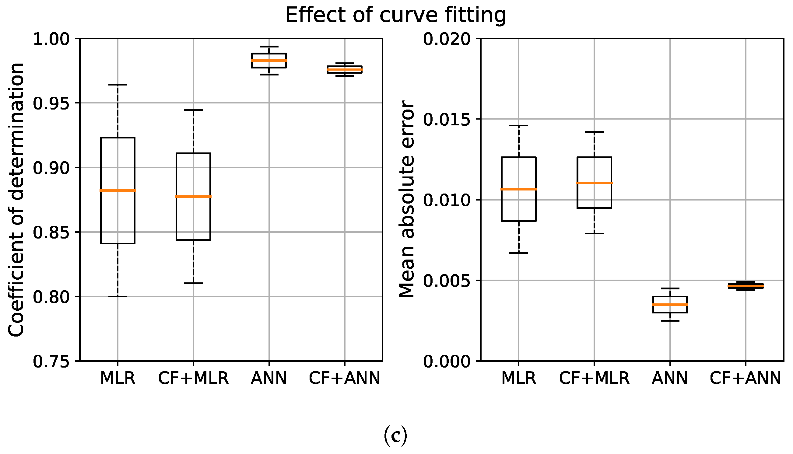
8	0.9808	0.0044

lists the predictive performance of the model cases using test data set, and Figure 8 compares the performance of the models according to the modeling method, variable selection method, and the application of curve fitting. Box plots were used to facilitate the observation of the distribution of the model performance, where the bottom and top of the box represent the first quartile (Q1) and third quartile (Q3), respectively, and the horizontal line within the box is the median. The top and bottom error bars represent the Q1 − 1.5 × IQR (interquartile range between Q1 and Q3) and Q3 + 1.5 × IQR of the data, respectively.

As shown in the figure, among the ANN model cases, Cases 3 and 7 had the highest accuracy with $R^2$ values of 0.9720 and 0.9936, respectively. Among the regression-based models, the $R^2$ values of Cases 2 and 5 were 0.8103 and 0.9641, respectively. Figure 8a,b prove that the ANN model rather than the regression model, and the LASSO regularization rather than the domain-knowledge method, respectively, provide better overall prediction performance. This study aimed to consider the nonlinear relationship between independent variables and the dependent variable in the linear regression model through a variable transformation using curve fitting. Referring to Table 8 and Figure 8c, some improvements were achieved in the prediction accuracy of the linear regression model when applying curve fitting. In contrast, ANN models showed poorer performance by applying curve fittings, as the nonlinearity was sufficiently described by the hidden layer.

3.2. Time-Series Analysis

In Section 3.1, the performance of the model against the test data set, which was randomly extracted from the data set regardless of ballast or laden voyage, was validated. To validate the performance of the model on the voyage unit, the fuel consumption efficiency over time for independent voyage data that has not been used to train and test the model so far was predicted in this Section. As shown in Figure 9, the target vessel sailed from Yantian to Singapore over a period of about 3 days. The analysis was conducted using data from the operating section of the voyage, from the point where the ship raised the engine power outside the harbour to the point of lowering the engine load before entering the destination port.

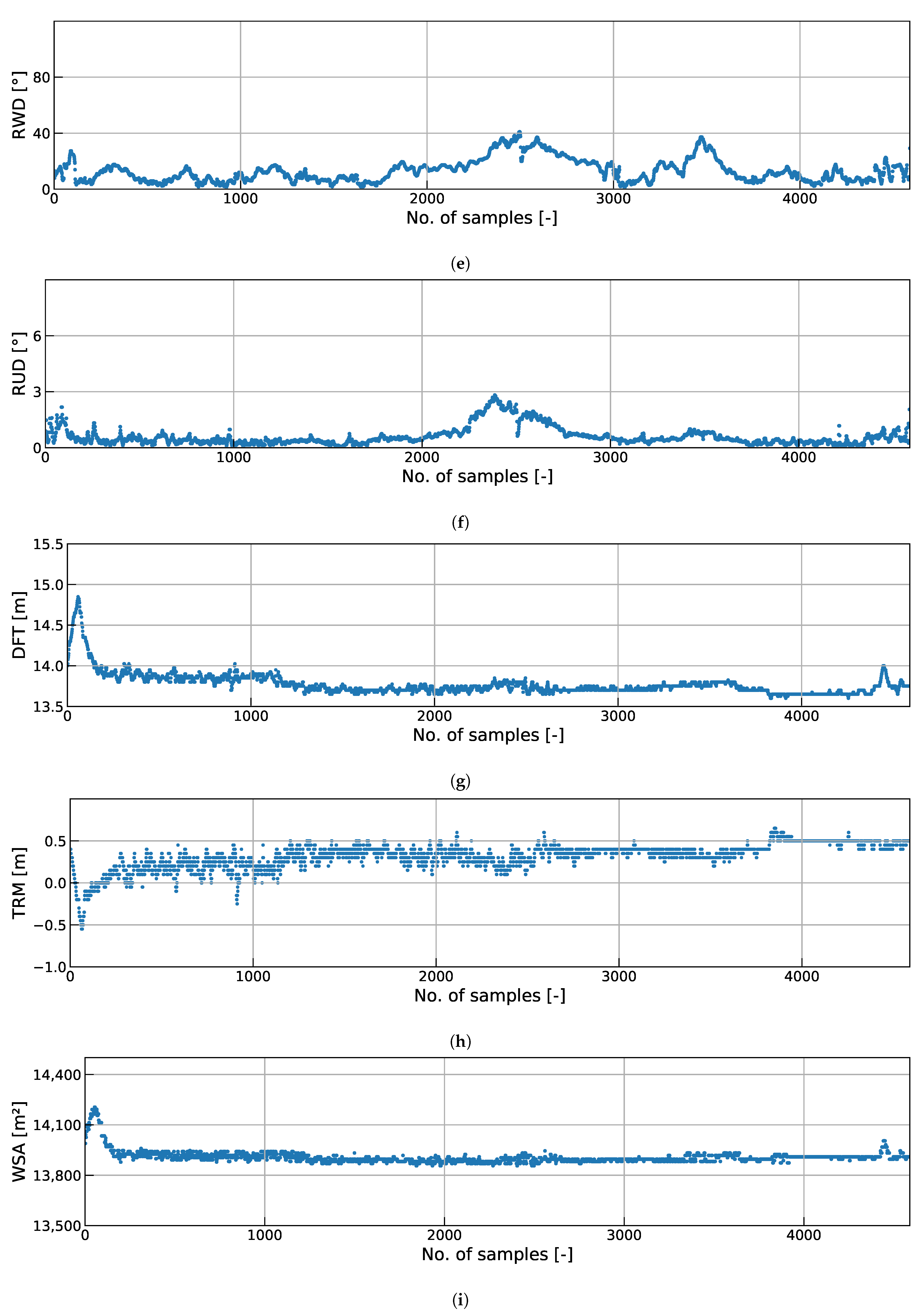
Figure 10 shows time-series data of the main engine RPM, SOG, STW, RWS, RWS, RUD, DFT, TRM, WSA, and DBS, while Figure 11 depicts the predicted fuel efficiency during the corresponding period using the models of Cases 2, 3, 5, and 7. The prediction results of Cases 2, 3, 5, and 7 follow the overall trend in actual fuel consumption efficiency, but some discrepancies were observed in the regions of 2200–2700 and 3800–4300. It was observed that the RWS of the corresponding section was somewhat stronger than that of other sections and that the vessel changed its RPM considerably in a short time. Therefore, the discrepancy between these actual and predicted values could be minimized by adding sufficient weather information for the navigational areas, such as wave and ocean currents, and processing data on the unsteady-state of the vessel operation, such as changes in the ship speed and course.

Over the 1414.85 nautical miles sailed by the target ship from Yantian to Singapore, the actual fuel consumption was 445.8 tons. The model with Cases 2, 3, 5, and 7 predicted values of 413.6, 436.0, 431.0, and 453.5 tons, respectively, i.e., prediction errors from −7.3% to 1.7%. Among them, Cases 3 and 7 using ANN had the lowest errors of −2.2% to 1.7%, with $R^2$ values above 0.97. Therefore, the use of ANN after selecting variables with domain-knowledge and LASSO regularization is considered the best method for predicting the fuel efficiency of the ship. The prediction results of these models are expected to be sufficiently accurate for predicting the energy efficiency of a vessel and can assist the operator in selecting suitable voyage variables for optimizing fuel efficiency.

3.3. Sensitivity Analysis on the Ship Draught

In the regression model, it is easy to identify the influence of the independent variable on the dependent variable from the regression coefficient. In contrast, since the ANN model is a complex mathematical model, it is difficult to interpret the developed model itself and get insight from it. Therefore, in this study, we wanted to interpret the results of the model by identifying the sensitivity from the output changes according to the input. The one-factor-at-a-time (OAT) method [52,53], which quantifies the variations in the output while keeping the other input variables as constants and changing only one target variable independently, was used to evaluate the local sensitivities of the ANN models.

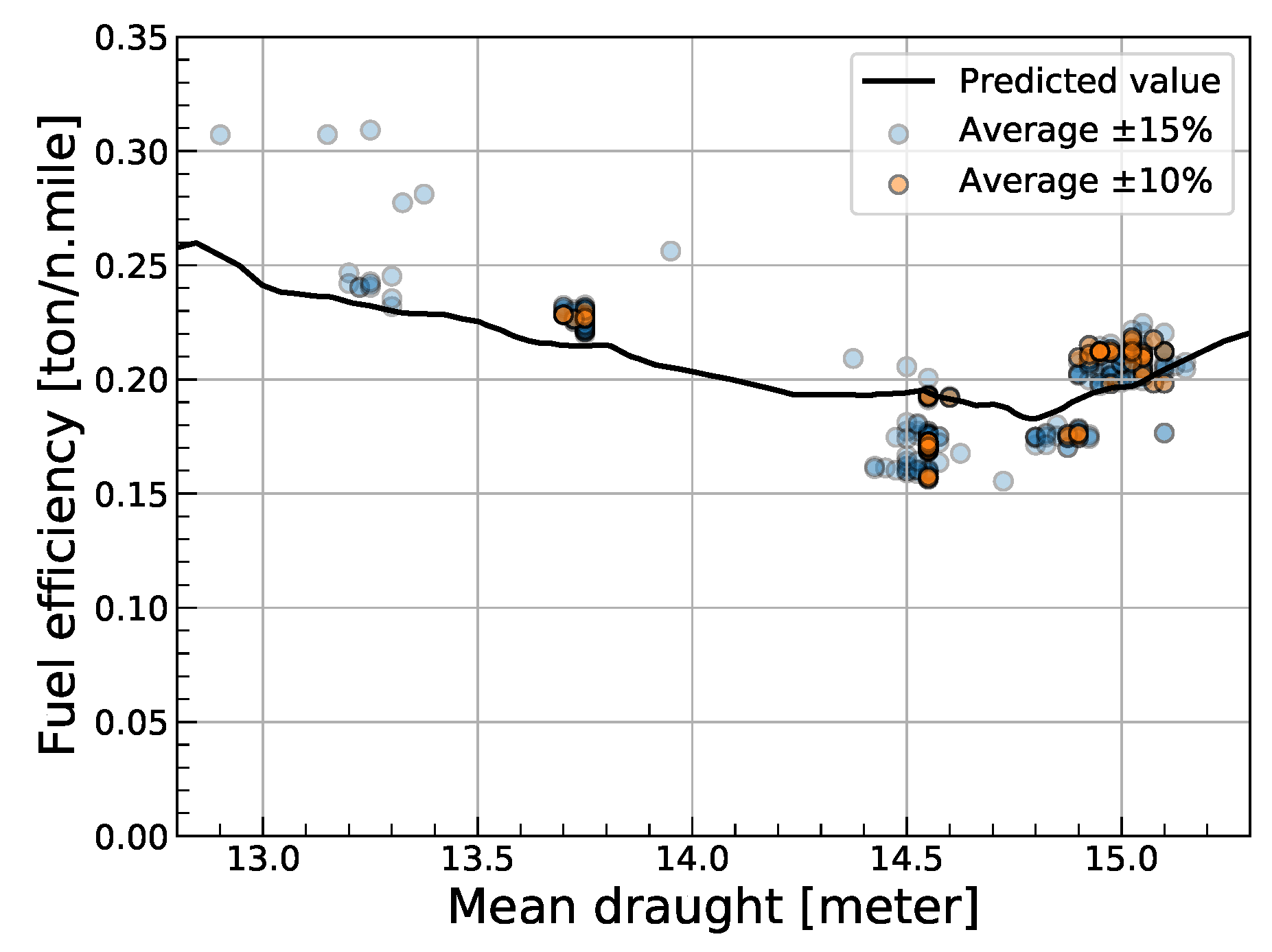
To verify the applicability and effectiveness of sensitivity analysis, a sensitivity analysis on the draught data of the ship was performed, and among the ANN models, case 3, which includes draught as an input variable, was used. The other input variables used in the model were fixed to the average operating conditions, while the draught was increased from its minimum to maximum value, and the final predicted fuel efficiency values were observed, as shown by the solid line in Figure 12. The blue and orange data points are the observed fuel efficiency when the range of each variable from the average operating condition is within 15%, and 10%, respectively. Under the average operating conditions of the ship, the draught resulting in the most efficient fuel consumption was predicted as 14.79 m. The design draught of the target ship is 14.50 m, which is usually designed for economically optimal operation. Hence, the prediction of the model very closely reproduces the draught required for the optimal operational performance of the ship. The optimal draught obtained from this study could be verified by computational fluid dynamics (CFD) or experiments with scale models of the ship. Then, the results of the model built from the in-service data could provide a new methodology for establishing optimal operating conditions for eco-friendly vessels.

4. Conclusions

The development of the fuel consumption prediction models with in-service data collected from a 13,000 TEU class container ship provided the following insights:

• The inconsistent nature of the ship operation data sets required the identification of outliers and smoothing of the data. The time-series graph proved that the identified outliers deviated from the overall data trend.
• Unlike other studies that used the amount of fuel consumed per unit time as a dependent variable, this study adopted fuel consumption per unit distance as a dependent variable for the fuel efficiency prediction model to complement previous research.
• The domain-knowledge method and LASSO regularization methods resulted in the selection of different input variables for the prediction model, where the latter resulted in the selection of more variables. When LASSO regularization was performed after curve fitting, fewer variables were selected.
• The best overall prediction performance was achieved using the ANN model (rather than the regression one) and using the LASSO regularization (rather than the domain-knowledge method). Among the model cases implemented in the study, those using ANN after selecting variables with domain-knowledge and LASSO regularization had the smallest prediction error compared with actual fuel consumption and are recommended for predicting the fuel consumption.
• When curve fitting was applied, the prediction accuracy of the linear regression model increased, while a poorer performance was observed for ANN models as the nonlinearity was reflected through the hidden layer.
• Sensitivity analysis on the ship draught allowed further analysis of the energy efficiency and identification of an optimal draught value, which was very similar to the design draught of the target vessel.

As the operational status of the ship and weather information in the sailing area is included in the model, the ship’s navigator can compare the energy efficiency for different operating conditions, such as optimal draught and trim values, and identify an optimal route for minimizing fuel consumption considering the weather during the voyage.

Further analyses of various voyage scenarios including navigational routes and operating environments are required to advance the model, and comparisons with CFD or model tests in similar conditions are required to reduce the gaps between the results obtained using fluid mechanics for ship design and data-driven models for eco-friendly vessels. In addition, more accurate predictions are expected if detailed weather data, including observations from ships, can be integrated into the model as an environmental load factor. As the periods of heave and pitch motions of the typical commercial vessel are much shorter than one minute [54,55], there has been a limitation on the comprehensive capture of the motion characteristics of the vessel according to the weather conditions at sea using in-service data at one-minute intervals. It is clear that the model can become more robust if the finer data set is acquired and converted into spectra to reflect the statistical characteristics (spectral moment) of the ship’s motion.

References

- Olmer, N.; Comer, B.; Roy, B.; Mao, X.; Rutherford, D. Greenhouse Gas Emissions from Global Shipping, 2013–2015; ICCT (The International Council on Clean Transportation): Washington, DC, USA, 2017. [Google Scholar]
- Committee, M.E.P. Guideline for Voluntary Use of the Ship Energy Efficiency Operational Indicator (EEOD); International Maritime Organization: London, UK, 2009. [Google Scholar]
- International Maritime Organization Resolution MEPC; International Maritime Organization: London, UK, 2018; Volume 304.
- Haites, E. Carbon taxes and greenhouse gas emissions trading systems: What have we learned? Clim. Policy 2018, 18, 955–966. [Google Scholar] [CrossRef] [Green Version]
- Gu, Y.; Wallace, S.W.; Wang, X. Integrated maritime fuel management with stochastic fuel prices and new emission regulations. J. Oper. Res. Soc. 2019, 70, 707–725. [Google Scholar] [CrossRef]
- Barnard, B. Maersk says slow steaming here to stay. J. Commer. Online 2011. Available online: http://www.joc.com/maritime/maersk-says-slow-steaming-here-stay (accessed on 9 September 2020).
- Eide, M.S.; Longva, T.; Hoffmann, P.; Endresen, Ø.; Dalsøren, S.B. Future cost scenarios for reduction of ship CO2 emissions. Marit. Policy Manag. 2011, 38, 11–37. [Google Scholar] [CrossRef]
- Branch, A.; Stopford, M. Maritime Economics; Routledge: Abington upon Thames, UK, 2013. [Google Scholar]
- ABS. Ship Energy Efficiency Measures Advisory. Available online: https://ww2.eagle.org/content/dam/eagle/advisories-and-debriefs/ABS_Energy_Efficiency_Advisory.pdf (accessed on 9 September 2020).
- Hellio, C.; Yebra, D. Advances in Marine Antifouling Coatings and Technologies; Elsevier: Amsterdam, The Netherlands, 2009. [Google Scholar]
- Schultz, M.; Bendick, J.; Holm, E.; Hertel, W. Economic impact of biofouling on a naval surface ship. Biofouling 2011, 27, 87–98. [Google Scholar] [CrossRef]
- Turan, O.; Demirel, Y.K.; Day, S.; Tezdogan, T. Experimental determination of added hydrodynamic resistance caused by marine biofouling on ships. In Proceedings of the 6th European Transport Research Conference, Warsaw, Poland, 18–21 April 2016; pp. 1–10. [Google Scholar]
- Beşikçi, E.B.; Arslan, O.; Turan, O.; Ölçer, A.I. An artificial neural network based decision support system for energy efficient ship operations. Comput. Oper. Res. 2016, 66, 393–401. [Google Scholar] [CrossRef] [Green Version]
- Kim, K.J.; Lee, S.D.; Jun, C.H.; Park, K.M.; Byeon, S.S. A statistical procedure of analyzing container ship operation data for finding fuel consumption patterns. Korean J. Appl. Stat. 2017, 30, 633–645. [Google Scholar] [CrossRef]
- Coraddu, A.; Oneto, L.; Baldi, F.; Anguita, D. Vessels fuel consumption forecast and trim optimisation: A data analytics perspective. Ocean Eng. 2017, 130, 351–370. [Google Scholar]
- Wang, S.; Ji, B.; Zhao, J.; Liu, W.; Xu, T. Predicting ship fuel consumption based on LASSO regression. Transp. Res. Part Transp. Environ. 2018, 65, 817–824. [Google Scholar] [CrossRef]
- Gkerekos, C.; Lazakis, I.; Theotokatos, G. Machine learning models for predicting ship main engine Fuel Oil Consumption: A comparative study. Ocean Eng. 2019, 188, 106282. [Google Scholar] [CrossRef]
- Yuan, J.; Nian, V. Ship energy consumption prediction with Gaussian process metamodel. Energy Procedia 2018, 152, 655–660. [Google Scholar] [CrossRef]
- Jeon, M.; Noh, Y.; Shin, Y.; Lim, O.K.; Lee, I.; Cho, D. Prediction of ship fuel consumption by using an artificial neural network. J. Mech. Sci. Technol. 2018, 32, 5785–5796. [Google Scholar] [CrossRef]
- Uyanik, T.; Arslanoglu, Y.; Kalenderli, O. Ship Fuel Consumption Prediction with Machine Learning. In Proceedings of the 4th International Mediterranean Science and Engineering Congress, Antalya, Turkey, 25–27 April 2019. [Google Scholar]
- Hu, Z.; Jin, Y.; Hu, Q.; Sen, S.; Zhou, T.; Osman, M.T. Prediction of fuel consumption for enroute ship based on machine learning. IEEE Access 2019, 7, 119497–119505. [Google Scholar] [CrossRef]
- Farag, Y.B.; Ölçer, A.I. The development of a ship performance model in varying operating conditions based on ANN and regression techniques. Ocean Eng. 2020, 198, 106972. [Google Scholar] [CrossRef]
- Gujarati, D.; Porter, D. Multicollinearity: What happens if the regressors are correlated. Basic Econometrics, 4th ed.; McGraw-Hill: New York, NY, USA, 2003; pp. 363–364. [Google Scholar]
- Harrell, J.; Frank, E. Regression Modeling Strategies: With Applications to Linear Models, Logistic Furthermore, ordinal Regression, and Survival Analysis; Springer: Berlin/Heidelberg, Germany, 2015. [Google Scholar]
- Bakar, Z.A.; Mohemad, R.; Ahmad, A.; Deris, M.M. A comparative study for outlier detection techniques in data mining. In Proceedings of the 2006 IEEE Conference on Cybernetics and Intelligent Systems, Bangkok, Thailand, 7–9 June 2006; pp. 1–6. [Google Scholar]
- Hair, J.; Babin, B.; Anderson, R.; Black, W. Multivariate Data Analysis, 8th ed.; Cengage Learning EMEA: Andover, UK, 2018. [Google Scholar]
- Yu, E.; Park, K.; Mun, D. Study on Prediction of Ship Navigation Efficiency Using Open Source-based Big Data Platform. Korean J. Comput. Des. Eng. 2018, 23, 275–284. [Google Scholar] [CrossRef]
- Soares, C.G.; Dias, S. Probabilistic models of still-water load effects in containers. Mar. Struct. 1996, 9, 287–312. [Google Scholar] [CrossRef]
- Ichinose, Y.; Tsujimoto, M.; Shiraishi, K.; Sogihara, N. Decrease of ship speed in actual seas of a bulk carrier in full load and ballast conditions. J. Jpn. Soc. Nav. Archit. Ocean. Eng. 2012, 15, 37–45. [Google Scholar] [CrossRef] [Green Version]
- Pratt, W.K. Introduction to Digital Image Processing; CRC Press: Boca Raton, FL, USA, 2013. [Google Scholar]
- Pedersen, B.P.; Larsen, J. Prediction of full-scale propulsion power using artificial neural networks. In Proceedings of the 8th International Conference on Computer and IT Applications in the Maritime Industries (COMPIT’09), Budapest, Hungary, 10–12 May 2009; pp. 10–12. [Google Scholar]
- Perera, L.P.; Mo, B. Marine engine operating regions under principal component analysis to evaluate ship performance and navigation behavior. IFAC-PapersOnLine 2016, 49, 512–517. [Google Scholar] [CrossRef]
- IMO. Guidelines for Voyage Planning; IMO: London, UK, 1999; Volume 893. [Google Scholar]
- Bowditch, N. American Practical Navigator-Bowditch; Paradise Cay Publications: Blue Lake, CA, USA, 2010. [Google Scholar]
- Du, Y.; Meng, Q.; Wang, S.; Kuang, H. Two-phase optimal solutions for ship speed and trim optimization over a voyage using voyage report data. Transp. Res. Part B Methodol. 2019, 122, 88–114. [Google Scholar] [CrossRef]
- Amini, M.; Roozbeh, M. Optimal partial ridge estimation in restricted semiparametric regression models. J. Multivar. Anal. 2015, 136, 26–40. [Google Scholar]
- Ferrero, P.; Iacovoni, A.; D’Elia, E.; Vaduganathan, M.; Gavazzi, A.; Senni, M. Prognostic scores in heart failure—Critical appraisal and practical use. Int. J. Cardiol. 2015, 188, 1–9. [Google Scholar] [CrossRef]
- Armstrong, V.N. Vessel optimisation for low carbon shipping. Ocean Eng. 2013, 73, 195–207. [Google Scholar] [CrossRef]
- Solas Chapter, V. Safety of Navigation. 1 July 2002. Available online: https://www.gov.uk/government/uploads/system/uploads/attachment-data/file/343175/solas-v-on-safety-of-navigation.pdf (accessed on 9 September 2020).
- Pierson, W.J., Jr.; Moskowitz, L. A proposed spectral form for fully developed wind seas based on the similarity theory of SA Kitaigorodskii. J. Geophys. Res. 1964, 69, 5181–5190. [Google Scholar] [CrossRef]
- Bales, S.L.; Lee, W.T.; Voelker, J.M. Standardized Wave and Wind Environments for NATO Operational Areas; Technical Report; David w Taylor Naval Ship Research and Development Center Bethesda md Ship: Brussels, Belgium, 1981. [Google Scholar]
- Tan, S.G. Seakeeping considerations in ship design and operations. In Proceedings of the MARIN, Wageningen, Presented at Regional Maritime Conference, Report 635001-Paper, Jakarta, Indonesia, 7–8 November 1995. [Google Scholar]
- Adland, R.; Jia, H. Dynamic speed choice in bulk shipping. Marit. Econ. Logist. 2018, 20, 253–266. [Google Scholar] [CrossRef]
- Newman, J.N. Marine Hydrodynamics; The MIT Press: Cambridge, MA, USA, 2018. [Google Scholar]
- Hastie, T.; Tibshirani, R.; Wainwright, M. Statistical Learning with Sparsity: The Lasso and Generalizations; CRC Press: Boca Raton, FL, USA, 2015. [Google Scholar]
- Rosenblatt, F. The perceptron: A probabilistic model for information storage and organization in the brain. Psychol. Rev. 1958, 65, 386. [Google Scholar] [CrossRef] [PubMed] [Green Version]
- Cybenko, G. Approximation by superpositions of a sigmoidal function. Math. Control. Signals Syst. 1992, 5, 455. [Google Scholar]
- Hahnloser, R.H.; Sarpeshkar, R.; Mahowald, M.A.; Douglas, R.J.; Seung, H.S. Digital selection and analogue amplification coexist in a cortex-inspired silicon circuit. Nature 2000, 405, 947–951. [Google Scholar] [CrossRef] [PubMed]
- Glorot, X.; Bordes, A.; Bengio, Y. Deep sparse rectifier neural networks. In Proceedings of the Fourteenth International Conference on Artificial Intelligence and Statistics, Ft. Lauderdale, FL, USA, 11–13 April 2011; pp. 315–323. [Google Scholar]
- Chollet, F. Keras Documentation. Available online: https://keras.io/ (accessed on 9 September 2020).
- Kingma, D.P.; Ba, J. Adam: A method for stochastic optimization. arXiv 2014, arXiv:1412.6980. [Google Scholar]
- Saltelli, A.; Ratto, M.; Andres, T.; Campolongo, F.; Cariboni, J.; Gatelli, D.; Saisana, M.; Tarantola, S. Global Sensitivity Analysis: The Primer; John Wiley & Sons: Hoboken, NJ, USA, 2008. [Google Scholar]
- Pianosi, F.; Beven, K.; Freer, J.; Hall, J.W.; Rougier, J.; Stephenson, D.B.; Wagener, T. Sensitivity analysis of environmental models: A systematic review with practical workflow. Environ. Model. Softw. 2016, 79, 214–232. [Google Scholar] [CrossRef]
- ABS. Guide for ’Safehull-Dynamic Loading Approach’ for Vessels. Available online: https://ww2.eagle.org/content/dam/eagle/rules-and-guides/current/design_and_analysis/140_safehulldlaforvessels/DLA-Vessels_Guide_e-May18.pdf (accessed on 9 September 2020).
- DNV. Classification Notes: CSA-Direct Analysis of Ship Structures. Available online: http://rules.dnvgl.com/docs/pdf/DNV/cn/2013-01/CN34-1.pdf (accessed on 9 September 2020).
- Yan, X.; Wang, K.; Yuan, Y.; Jiang, X.; Negenborn, R.R. Energy-efficient shipping: An application of big data analysis for optimizing engine speed of inland ships considering multiple environmental factors. Ocean Eng. 2018, 169, 457–468. [Google Scholar] [CrossRef]
Figure 1.
Outlier detection using the relationship between fuel consumption and engine power.
Figure 2.
Trend of main engine power and fuel consumption data around sampling point.
Figure 3.
Time-series data filtered by median filter: (a) Mean draught, (b) Trim.
Figure 4.
Curve fitting of ship parameters: (a) RPM, (b) STW, (c) SOG, (d) RWS, (e) RWD, (f) RUD, (g) DFT, (h) TRM, (i) DIS, (j) WSA, (k) DBS.
Figure 5.
Geometric interpretation of LASSO regression.
Figure 6.
Architecture of a multilayer perceptron.
Figure 7.
Effect of changing the number of hidden neurons and layers on R2: (a) Case 3, (b) Case 4, (c) Case 7, and (d) Case 8.
Figure 8.
Box plots of prediction performance for model cases: (a) modeling method, (b) variable selection method, (c) effect of curve fitting.
Figure 9.
Navigational route of the target ship.
Figure 10.
Ship parameters collected during a voyage from Yantian to Singapore: (a) RPM, (b) SOG, (c) STW, (d) RWS, (e) RWD, (f) RUD, (g) DFT, (h) TRM, (i) WSA, (j) DBS.
Figure 11.
Prediction results of developed models for the time-series data.
Figure 12.
Sensitivity analysis of DFT under average operating conditions of the ship.