
Small Floating Target Detection Method Based on Chaotic Long Short-Term Memory Network


1
Collaborative Innovation Center on Forecast and Evaluation of Meteorological Disasters, Nanjing University of Information Science and Technology, Nanjing 210044, China
2
Jiangsu Key Laboratory of Meteorological Observation and Information Processing, Nanjing University of Information Science and Technology, Nanjing 210044, China
*
Author to whom correspondence should be addressed.
J. Mar. Sci. Eng. 2021, 9(6), 651; https://doi.org/10.3390/jmse9060651
Submission received: 6 May 2021
/
Revised: 29 May 2021
/
Accepted: 1 June 2021
/
Published: 12 June 2021
(This article belongs to the Special Issue Artificial Intelligence in Marine Science and Engineering)
Abstract
:In order for the detection ability of floating small targets in sea clutter to be improved, on the basis of the complete ensemble empirical mode decomposition (CEEMD) algorithm, the high-frequency parts and low-frequency parts are determined by the energy proportion of the intrinsic mode function (IMF); the high-frequency part is denoised by wavelet packet transform (WPT), whereas the denoised high-frequency IMFs and low-frequency IMFs reconstruct the pure sea clutter signal together. According to the chaotic characteristics of sea clutter, we proposed an adaptive training timesteps strategy. The training timesteps of network were determined by the width of embedded window, and the chaotic long short-term memory network detection was designed. The sea clutter signals after denoising were predicted by chaotic long short-term memory (LSTM) network, and small target signals were detected from the prediction errors. The experimental results showed that the CEEMD-WPT algorithm was consistent with the target distribution characteristics of sea clutter, and the denoising performance was improved by 33.6% on average. The proposed chaotic long- and short-term memory network, which determines the training step length according to the width of embedded window, is a new detection method that can accurately detect small targets submerged in the background of sea clutter.
1. Introduction
Weak signal detection technology has been applied in many engineering fields, such as radar detection [1], medical signal extraction [2,3], fault diagnosis [4,5,6], etc. The above signal energy is generally weak and contains noise, and the way in which to detect weak signals while accurately denoising has always been a research hotspot.
Sea clutter [7] is the backscattering echo of radar signals emitted by local sea level, which is affected by multiple factors such as sea wind and waves. In 1998, Huang et al. [8] proposed empirical mode decomposition (EMD), which is an adaptive time–frequency analysis method adapted to non-stationary signals that has attracted great attention in signal processing research. Yeh et al. [9] proposed a complementary ensemble empirical mode decomposition (CEEMD) method. Zhang et al. [10] proposed a new combination model based on complementary empirical mode decomposition, T-S fuzzy neural network (FNN) optimized by improved genetic algorithm (IGA) and Markov error correction, to improve the accuracy of ultra-short-term wind power prediction. Ji et al. [11] proposed the CEEMD-LSSVM model and proved that it had a great advantage in the forecasting of inflow runoff during the wet season. Huang et al. [12] used power spectral density, correlation coefficient, and variance contribution rate analysis methods to select IMF components containing effective information and reconstructing signals for denoising. Aiming at the non-stationary nonlinear characteristics of sea clutter, the design of appropriate IMF selection method is the key research problem.
In recent years, researchers represented by Haykin et al. [13] have analyzed a large number of measured data at sea and have confirmed that sea clutter is not a completely random signal but has typical chaotic characteristics. Domestic and foreign researchers have used various methods to construct prediction models for chaotic time series prediction, including multiple linear regression method, Fourier expansion method, support vector machine, artificial neural network, and so on. Among them, back propagation (BP) neural network is widely used as a typical network in artificial intelligence methods. Xing et al. [14] used BP neural network to detect weak signals in chaotic background. With the increasing requirement of detection accuracy, the shortcomings of BP neural network, such as simple structure and poor learning ability, are gradually exposed.
Lately, more and more scholars have paid attention to the field of deep learning. Among many deep learning models, recurrent neural network (RNN) introduces the concept of timing sequence into the network structure design, which makes it more adaptable in the analysis of timing sequence data. Wu et al. [15] proposed a new method for fault prediction of equipment degradation sequence based on long short-term memory (LSTM) network, conducted experiments on the challenge data set from the first International Conference on PHM (Denver, CO, USA). Amir et al. [16] used LSTM network to detect mooring line faults and proved through experiments that the prediction effect of LSTM was better than that of multilayer perceptrons. Balogun et al. [17] used deep learning techniques to integrate a wide range of ocean–atmospheric variables to predict sea level changes along the coastline of the western peninsula of Malaysia.
In this paper, we studied the intrinsic mode function (IMF) decomposed by complete ensemble empirical mode decomposition (CEEMD) and used the autocorrelation function of each IMF to segment the low-frequency IMF and the high-frequency IMF; the correctness of the separation method was judged by the agreement between the IMF energy ratio curve and the range gate distribution characteristics of sea clutter, the low-frequency IMFs are regarded as the main signal component, and the high-frequency IMFs are regarded as the noisy signal for wavelet packet transform denoising and use the measured sea clutter data to verify the universality of the proposed new method of selecting IMF. We combined the chaotic characteristics of sea clutter with long short-term memory (LSTM) networks, used the phase space reconstruction technique to reconstruct the original motion trajectory of chaotic sea clutter, and obtained the embedded window width of sea clutter data by the C-C method [18]. We set the width of the embedded window as the training timesteps in the long short-term memory network to predict the sea clutter signal, detect small targets from the prediction error, and verify the detection efficiency of the chaotic long short-term memory network through experiments.
2. CEEMD-WPT Denoising Algorithm
The CEEMD algorithm is a time–frequency signal processing method based on adaptive orthogonal basis. When using CEEMD to denoise sea clutter, there is no need to analyze and study in advance, and thus it can be decomposed directly. After decomposing into a series of intrinsic mode functions, the high-frequency IMF and low-frequency IMF are separated by autocorrelation function, and we calculate the autocorrelation function of each IMF. According to the characteristics of autocorrelation function between signal and noise, the signal has strong correlation, and the value of its non-zero autocorrelation function will change with the change of time difference. Noise has randomness and weak correlation at each moment, and the value of its autocorrelation function at non-zero point will decay rapidly and approach 0. According to the difference between the two, the frequency band can be effectively divided [19].
However, to judge whether the method of distinguishing high-frequency IMF and low-frequency IMF by autocorrelation function is accurate, we also need to calculate the energy proportion of IMFs with noise and compare the range gate distribution characteristic of sea clutter. If the two characteristics match, the high and low frequencies of the IMFs are considered to be properly separated. The low frequency IMFs are considered as the main signal part, and the high frequency IMFs are considered as the noisy signal for wavelet packet transform de-noising, while the denoised high-frequency IMFs and the main signal IMFs are reconstructed into a pure signal. The implementation steps are as follows:
1. groups of auxiliary white noise are added to the original sea clutter signal, and the auxiliary white noise is added in the form of positive and negative pairs, so as to generate two sets of IMF:
where is the original signal; is the auxiliary noise; and and are the signals added with positive and negative paired noise, respectively. Thus, the number of collective signals is 2n.
2. Each signal in the set is decomposed by empirical mode decomposition (EMD) [9], and each signal gets a group of IMF components in which the IMF component of the signal is expressed as .
3. The decomposition results are obtained by the combination of multiple components:
where is the IMF component obtained by CEEMD decomposition. Thus, the target signal can be expressed as
4. The autocorrelation function of each IMF component is calculated, high frequency IMF and low frequency IMF are distinguished by autocorrelation function characteristics, and whether the energy proportion curve of high frequency IMF is consistent with the range gate distribution characteristics of sea clutter is determined. If so, the first E IMFs are classified as high-frequency part:
5. It is considered that are high-frequency noisy signals, and they are denoised by wavelet packet:
Wavelet packet decomposition algorithm:
Wavelet packet reconstruction algorithm:
where d is the wavelet packet decomposition coefficient, and are the filter coefficients, and are the number of decomposition layers, and and are the node number of wavelet packets.
6. The denoised data and low-frequency IMF components are used to reconstruct the original signal, that is, the required pure signal.
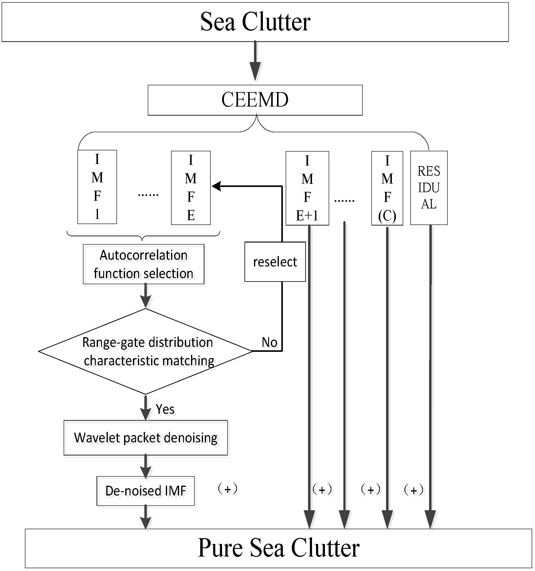
The proposed CEEMD-WPT denoising algorithm flow chart is shown in Figure 1.
As shown in Figure 1 above, we propose that in practical engineering applications, the sea clutter with noise is processed by CEEMD to obtain a series of IMF components arranged from high frequency to low frequency after decomposition. Since CEEMD is a data-driven decomposition algorithm, the number of IMF components is determined by the data length and data characteristics, generally between 9 and 11. IMF(c) is used to represent this uncertainty. The IMFs are divided into low-frequency and high-frequency parts by the autocorrelation function. The energy proportion of IMFs with noise is calculated and then compared with the range gate distribution characteristic of sea clutter, and the consistency of the results is used to judge whether the method of distinguishing high-frequency IMF and low-frequency IMF by autocorrelation function is accurate. The low-frequency part is set as the main signal component, and the high-frequency part is set as the noisy signal for wavelet packet denoising. The processed IMFs and the unprocessed low-frequency IMFs are obtained to reconstruct the pure sea clutter data.
3. Chaotic Long- and Short-Term Memory Network
After preprocessing by CEEMD and wavelet packet transform, the pure sea clutter sequence is obtained. The nonlinear and nonstationary sea clutter signal has chaotic characteristics. Combined with the phase space reconstruction theory of chaotic system, the LSTM network prediction model of chaotic time series is designed.
3.1. LSTM Network
The sea clutter signal is divided into 14 groups of sea conditions. Each sea condition has 14 range gates, including main target range gate, secondary target range gate, and no target range gate. Each range gate contains 130,000 sampling points. For the complex signal of sea clutter, LSTM network processing is more suitable. LSTM introduces the concept of cell; adds “forgetting gate”, “input gate”, and “output gate” in the network; selectively retains the initial time information; solves the problem of low data utilization; and is more suitable for long time series processing. Complex back-propagation operations are performed by three “gates”. The workflow of three special gates in LSTM is described in detail as follows:
Forgetting gate: can selectively discard useless data. By using the output of the previous time and the input of the current time, and giving each data in the cell state of the previous time, a weight between 0 and 1, that is indicates the degree of retention, LSTM network can update this weight through continuous feedback learning to optimize the model.
In Equation (9), is the sigmoid activation function, is the weight matrix of the forgetting gate, and is the bias term of the forgetting gate.
Input gate: used to select information stored in cell state. It consists of two parts: the sigmoid layer decides what value needs to be updated, and the output is recorded as . The tanh layer generates new information , which is ready to be added into the cell state.
Then, the cell state is updated continuously, the cell state at the previous time is multiplied by the output function of forgetting gate, and the generated candidate new information is added:
Output gate: filter to confirm the output value in the cell state, which is also divided into two layers: sigmoid layer determines which part of the cell state is output, and its output is recorded as . The tanh layer normalized the updated cell state to between −1 and 1, and is output result.
3.2. LSTM Detection Method for Weak Signals in Chaotic Sequences
The prediction mechanism of LSTM network determines that the longer the training step is, the more accurate the prediction result will be. However, it is impossible to expand the training step without limited for sea clutter, which is a one-dimensional long sequence. It is necessary to make a trade-off between the prediction accuracy and the operation efficiency. A combined network is proposed, which can not only fully perform the data characteristics but can also take into account the operation efficiency and redundancy. The research shows that the sea clutter signals are chaotic time series, and the one-dimensional sea clutter data can be reconstructed into a set of high-dimensional vector series by phase space reconstruction theory, in which each row of vectors has topological similarity with the original data. Therefore, we propose the use of the high-dimensional array structure in phase space reconstruction to determine the training step size of LSTM.
For the chaotic sea clutter sequence , the phase space is reconstructed by choosing the appropriate embedding dimension m and delay time , and a new set of vector sequences is obtained from .
It can be seen from the above formula that phase space reconstruction is to decompose one-dimensional data into n high-dimensional sequences of length m. Each high-dimensional sequence is equivalent to the original one-dimensional data in topological sense and has similarity. There are points in each column, and the chaotic prediction model is established from the reconstructed chaotic phase space.
Define embedded windows :
In the prediction of time series, the first K points are often used to predict the value of the K + 1 point after network learning.
Considering the chaotic characteristics of sea clutter and the long-term learning ability of long-term and short-term memory network, this method uses the embedded window to determine the training step K, so as to ensure that the first K points of training contain a column of vectors in Equation (15), which can not only avoid the operation redundancy caused by too long training step, but also ensure that the chaotic characteristics are not destroyed and more accurate prediction data can be obtained. The prediction model is as follows:
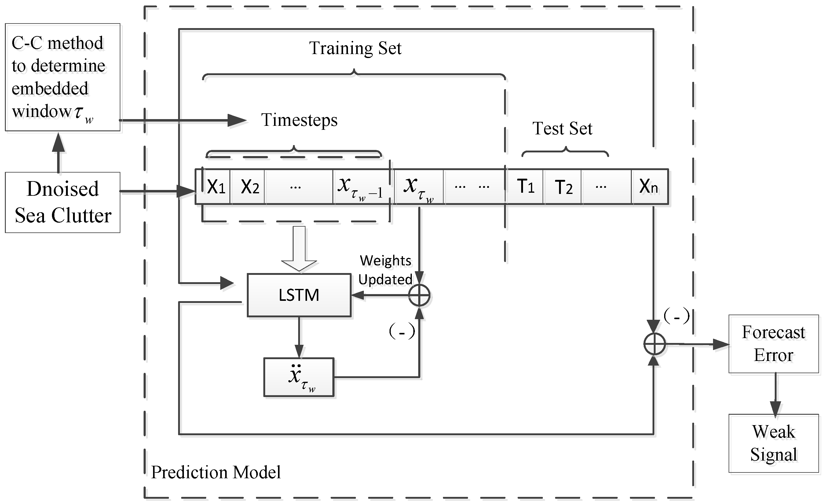
The designed chaotic long-term and short-term memory network uses as the input vector and as the target value for training, and uses sliding window to study the prediction problem as the supervised learning problem. The network parameters are adjusted by backward propagation, the dropout layer is set in the network to prevent overfitting, and the average square loss function is used for calculation. In the test, the loss function and optimization steps are calculated. Through the strong learning ability of neural network, the trained model will be very close to the actual dynamic system, so as to realize the reconstruction of chaotic system and complete the prediction of chaotic time series. Small targets are detected from the prediction error. The operation flow chart is shown in Figure 2.
As shown in the figure above, according to the chaotic characteristics of sea clutter, the prediction model of chaotic long short-term memory network is proposed. The embedding window is determined by C-C method [18], and the training step of the network is set to , so as to avoid operation redundancy and ensure the chaotic characteristics of sea clutter data, detecting small target signal from prediction error.
4. Experiment
4.1. Data Sources
In order to test the practicability of the weak signal detection method based on LSTM, we used the measured sea clutter data for experiments. The sea clutter data used in this paper was IPIX radar sea clutter data of McMaster University in Canada. In the HH polarization mode, there are 14 range gates for each of 14 sea conditions, a total of 196 sets of data, and each dataset contains 130,000 sampling points.
4.2. CEEMD-WPT Denoising Algorithm
After the original sea clutter signal is decomposed into a series of IMF by CEEMD, the low-frequency IMF is selected as the main signal part, and the high-frequency IMF is selected as the noisy signal for wavelet packet de-noising.
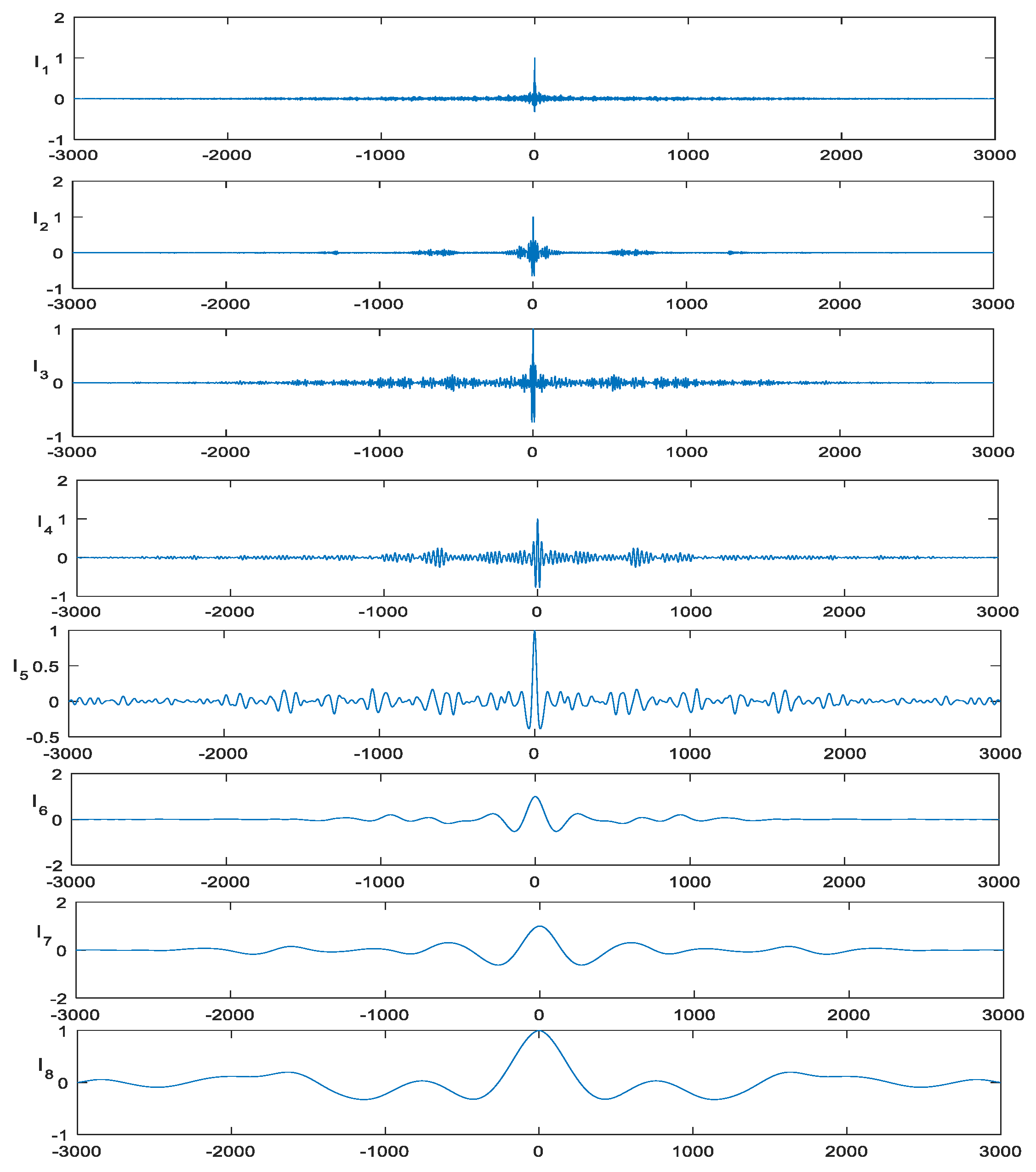
The first 3000 points of the ninth distance gate in #17 group of sea conditions were selected for experiment. After CEEMD decomposition, 9 IMFs and a trend term residt were obtained, as shown in Figure 3.
We used the autocorrelation function to separate high-frequency IMF and low-frequency IMF, and used the range gate distribution characteristics of sea clutter to verify the accuracy of the segmentation method.
The autocorrelation function of each IMF component was calculated, which is shown in Figure 4; the signal had strong correlation, and the autocorrelation function value of its non-zero point will change with the change of time difference. Noise had randomness and weak correlation at each moment, and its autocorrelation function value at non-zero point will decay rapidly and approach 0.
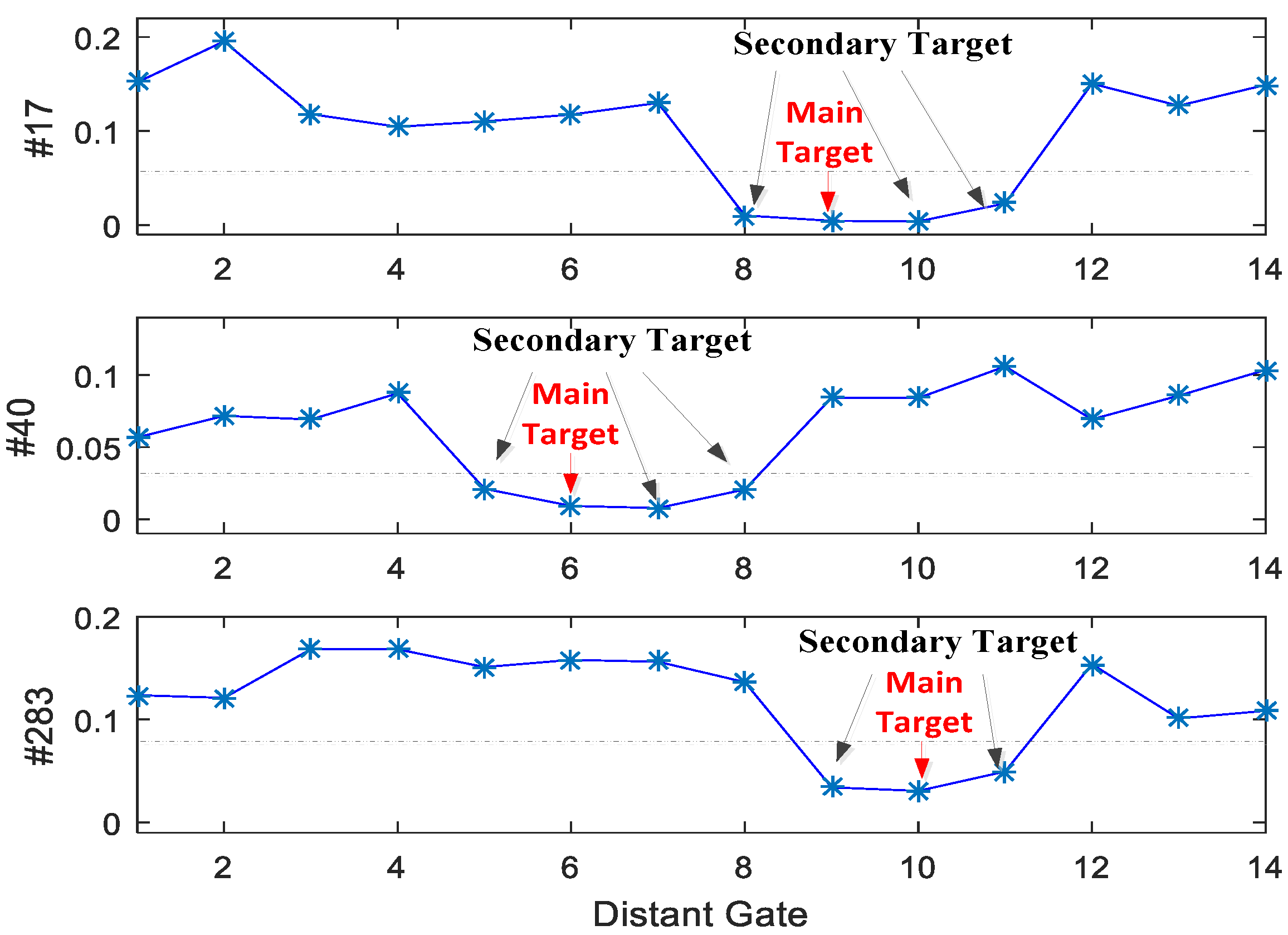
It can be seen from Figure 4 that IMF1–IMF5 can be considered as noise according to the autocorrelation function characteristics of signal and noise. In order to verify whether the method is correct, we calculated the energy proportions of the first five IMFs and compared them with the distance-gate distribution characteristics of this wave. The results are shown in Figure 5.
As can be seen from the above figure, the total energy proportion of IMF1–IMF5 varied greatly between the range gates with and without targets. Compared with the range gate without the target, the total energy proportion of the first five IMFs with the main target was reduced by an order of magnitude, and the energy proportion of the range gate with the secondary target was also greatly reduced. Therefore, it was reasonable and universal to select the first five IMFs as the high-frequency noise components for denoising.
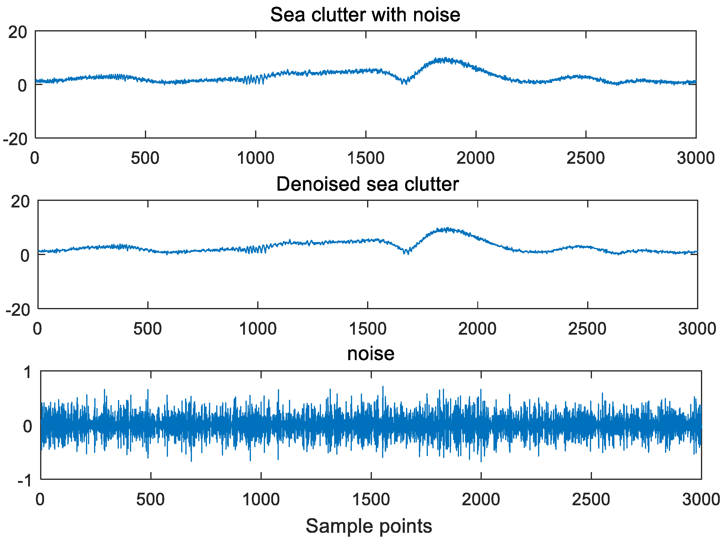
After IMF selection, IMF1–IMF5 were denoised by wavelet packet transform, and the low-frequency main signal IMFs were used to reconstruct the pure sea clutter signal. In order to compare the denoising effect, we added a 10 dB white noise into the sea clutter data, and the complementary ensemble empirical mode decomposition (CEEMD) and empirical mode decomposition (EMD) denoising algorithms were compared. The effectiveness of the proposed denoising algorithm was verified. The denoising signal is shown in Table 1, and the experimental results are shown in Figure 6.
According to Table 1, the signal-to-noise ratio (SNR) of CEEMD-WPT de-noising algorithm based on the new method of IMF extraction was the highest. SNR increased by an average of 33.6%. When it was combined with Figure 5, it was shown that the proposed algorithm not only had the same target distribution characteristics as sea clutter, but also had good de-noising effect and can be applied to practical engineering.
4.3. Chaotic Long-Term and Short-Term Memory Network
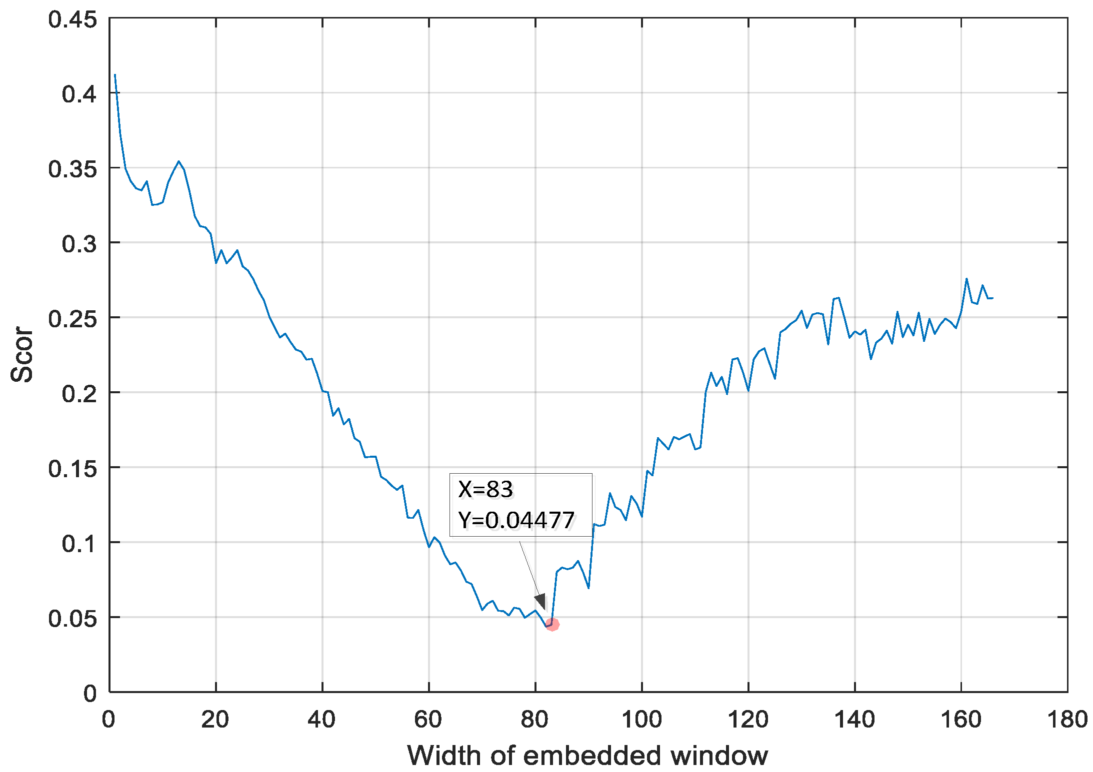
According to the chaotic characteristics of sea clutter, the embedding window of chaotic sea clutter sequence is obtained by the C-C method, which ensures that a chaotic period is included in a training step of chaotic long short-term network. The calculation experiment is carried out on #17 group of sea condition data. The experimental results are shown in Figure 7. The abscissa corresponding to the global minimum is the embedding window width of chaotic sequence.
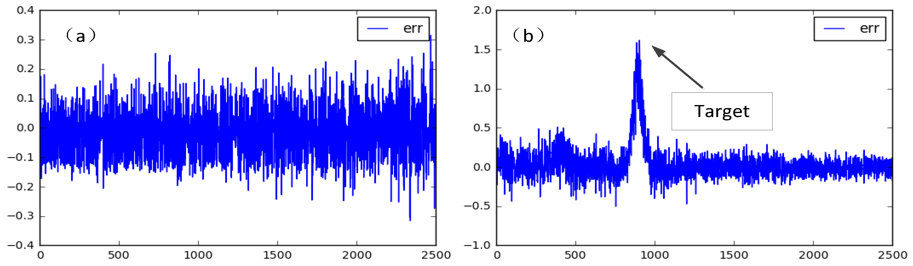
According to Figure 7, the embedding window was 83, which shows that in the one-dimensional sea clutter data, 83 points contained a set of high-dimensional sequences that had topological similarity with the original sea clutter data and can be used as the training step of long short-term memory network. The number of hidden layers of network parameters was 30, the batch size was 32, the training data were 10,000 points, and the test data were 2500 points, The first distance gate and the ninth distance gate of the #17 group of sea conditions after denoising were used for prediction, and the prediction results are shown in Figure 8.
As can be seen from Figure 8, after the chaotic long short-term memory network prediction, no small target was found in the prediction error of the first range gate, and the target signal was found in the prediction error of the ninth range gate, which was consistent with the target distribution characteristics of sea clutter. This showed that the chaotic long short-term memory network is accurate and effective in dealing with sea clutter.
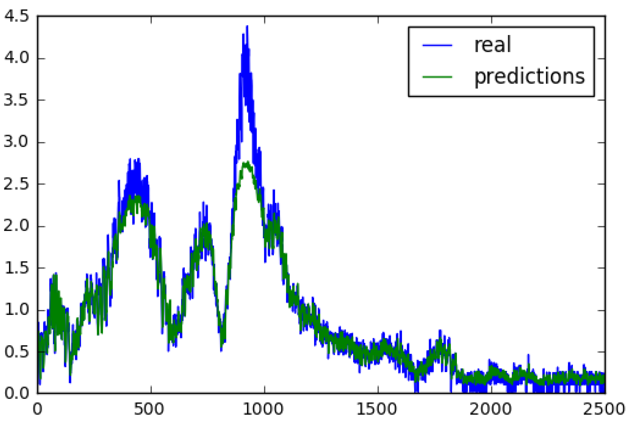
Considering that there may be overfitting problems in the network, we set the dropout layer in the network to randomly delete some neurons. It can be seen from Figure 9 that the designed chaotic long short-term memory network can learn the trend of sea clutter precisely.
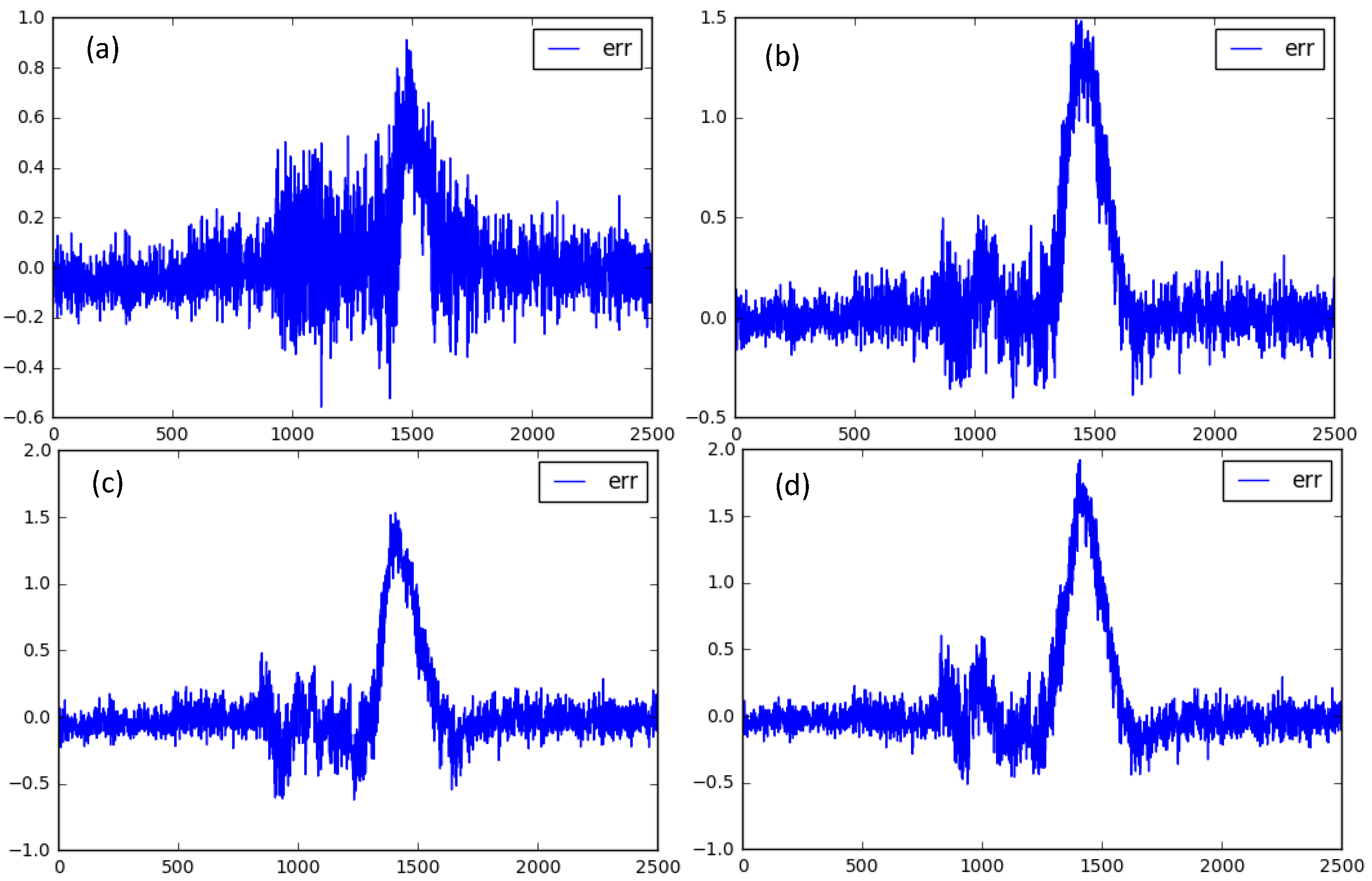
In order to verify the detection effect of determining the training step size of chaotic long short-term memory network by embedding window, we carried out the experiment on the sea clutter data with targets in the eighth range gate under #54 group of sea conditions. The experimental results are shown in the Figure 10.
It can be seen from Figure 10a that the training step of 10 selected in the past experience was very poor in predicting small and medium targets of #54 group of sea conditions. Through the reconstruction of chaotic phase space, we obtained the embedding dimension, and the training step was determined as 83. The experimental results are shown in Figure 10b. The existence of small targets can be clearly detected from the prediction error, which was greatly improved compared with Figure 10a. By further increasing the training step size, we are able to see in Figure 10c,d that the prediction accuracy was indeed improved, but the difference with Figure 10b was very small, which indicates that the training step size determined by the number of embedding windows met the needs of detection, which were able to effectively improve the operation efficiency while accurately detecting signals.
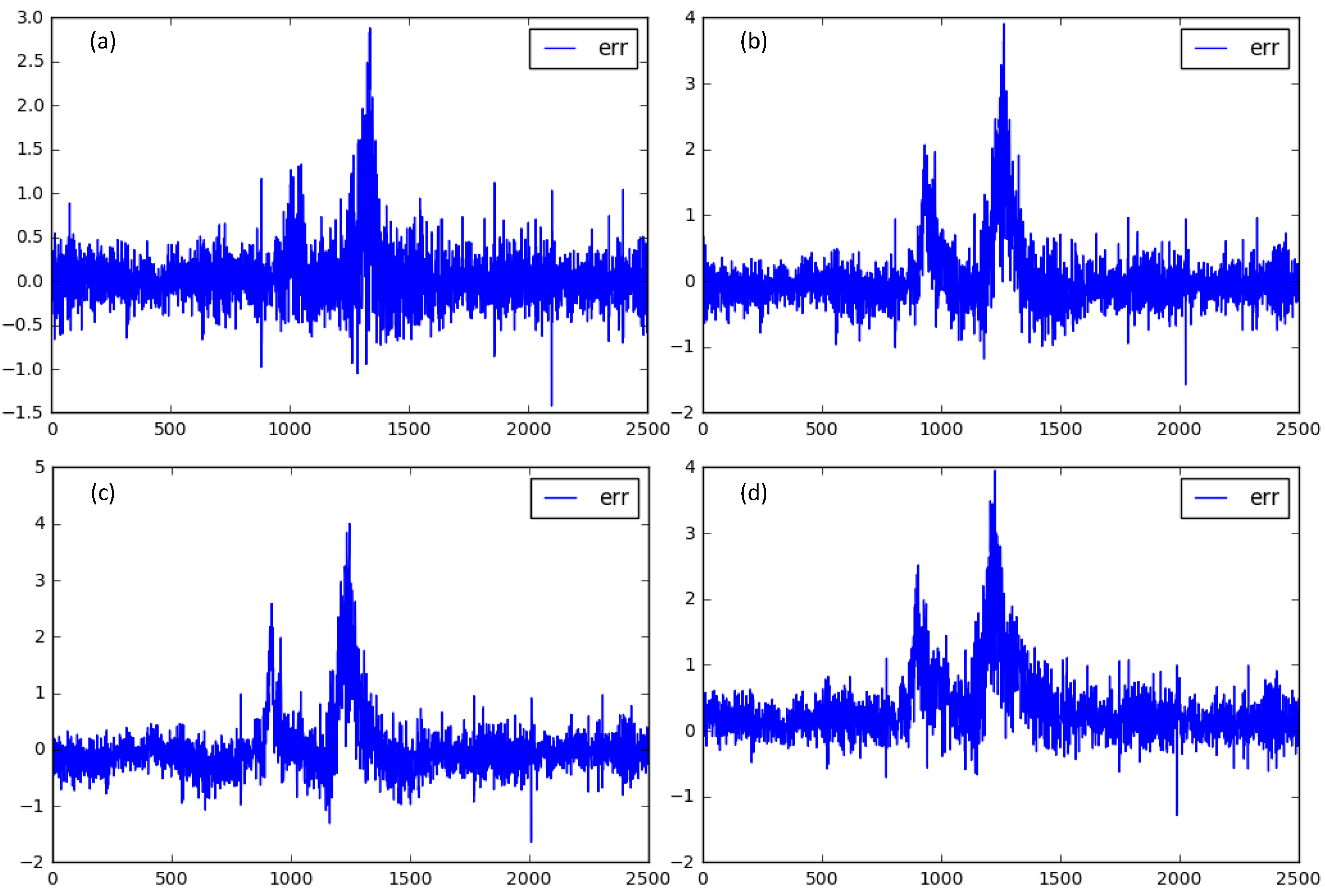
In order to avoid the adverse impact of accidental data on network model validation, we used seventh range gate sea clutter under #310 group of sea conditions for experiments, and the experimental results are shown in the Figure 11.
As can be seen from Figure 11a, a target signal can be detected in the prediction error. However, in Figure 11b, when the training step was 83, a small target with lower amplitude appeared on the left side of the main target, and the prediction network with training step of 10 was not detected. As can be seen from Figure 11c,d, when the training step was broadened to 100 and 120, another small target was also detected. However, the detection accuracy was not greatly improved, which showed that the proposed network improvement method to determine the training step through the embedded window was accurate and effective. The comparison table of prediction error of different training steps was as follows:
It can be seen from Table 2 that with the increase of training step, the prediction error was also increasing, which reflected the improvement of prediction accuracy. With the increase of training step, the proportion of prediction error decreased greatly, which indicates that the improvement of detection accuracy will decrease sharply when the training step increases to a certain value. It is not the case that the longer the training step, the better the network effect. It is necessary to consider the training speed while ensuring the detection accuracy.
5. Conclusions
In the study of how to accurately detect small floating targets on the sea, the detection process is usually divided into preprocessing and post-prediction processes. We also divided the research into two parts. In the data preprocessing part, we studied the latest denoising algorithm and used complete ensemble empirical mode decomposition (CEEMD) to decompose the data into a series of intrinsic mode functions (IMFs). According to the characteristics of sea clutter, we distinguished high frequency IMF and low frequency IMF by IMFs’ autocorrelation function and used the range gate distribution characteristics of sea clutter to verify the accuracy of the segmentation method. The total energy proportion of IMF1–IMF5 in each range gate dataset was consistent with the target distribution, and thus IMF5 was used as the separation line, and IMF1–IMF5 were considered as the high-frequency noise part for wavelet packet denoising. The residual component was not processed as the main signal component, and the pure sea clutter signal was reconstructed by denoised IMF1–IMF5 and the main signal component.
In order to improve the detection accuracy and operation efficiency, we designed a chaotic long short-term memory network detection model. The LSTM network training steps were determined by the width of the chaotic parameter embedding window of the sea clutter. A group of high-dimensional vectors were included in a training cycle. Small target signals were detected from the prediction error. The prediction results of different training steps were compared. The experimental results showed that the method of determining the training step size by embedding window width can not only detect the small target submerged in sea clutter more accurately, but also reduce the amount of computation and avoid computational redundancy. By combining the new preprocessing method with chaotic long short-term network, we designed a universal, efficient, and accurate detection method for floating small targets on the sea. The experimental results show that the new preprocessing algorithm performs well in denoising, and the designed chaotic long short-term network prediction is accurate and efficient.
The method proposed in this paper is not only effective for small target detection in the background of sea clutter, but also can be used for the prediction of long time series in other fields. In the next step, we are going to use the latest measured radar data, design an optimization algorithm to improve other LSTM network parameters, and establish an evaluation index based on deep learning detection mechanism.
Author Contributions
Conceptualization, Y.Y. and H.X.; methodology, H.X.; software, Y.Y. python 3.5.2, (1 June 2020); validation, Y.Y. and H.X.; formal analysis, H.X.; resources, H.X.; data curation, Y.Y.; writing—original draft preparation, Y.Y.; writing—review and editing, H.X. All authors have read and agreed to the published version of the manuscript.
Funding
This work is supported by the National Key R&D Program of China (Grant No. 2021YFE0105500), National Natural Science Foundation of China (Grant No. 61671248), and the 2019 Jiangsu Graduate Scientific Research Innovation Program (Grant No. SJKY19_0973).
Data Availability Statement
The data were downloaded from the following website: http://soma.ece.mcmaster.ca/ipix/index.html. (accessed on 27 May 2021), The data were measured with the McMaster IPIX Radar, a fully coherent X-band radar, with advanced features such as dual transmit/receive polarization, frequency agility, and stare/surveillance mode.
Conflicts of Interest
The authors declare that there is no conflict of interest regarding the publication of this paper.
References
- Lee, S.; Lee, J.Y.; Kim, S.C. Mutual Interference Suppression Using Wavelet Denoising in Automotive FMCW Radar Systems. IEEE Trans. Intell. Transp. Syst. 2021, 22, 887–897. [Google Scholar] [CrossRef]
- Yan, W.; Du, C.; Luo, D.; Wu, Y.; Duan, N.; Zheng, X.; Xu, G. Enhancing detection of steady-state visual evoked potentials using channel ensemble method. J. Neural Eng. 2021, 18, 046008. [Google Scholar] [CrossRef] [PubMed]
- Xiao, D.; Chen, Y.; Li, D.U. One-Dimensional Deep Learning Architecture for Fast Fluorescence Lifetime Imaging. IEEE J. Sel. Top. Quantum Electron. 2021, 27, 7000210. [Google Scholar] [CrossRef]
- Chen, H.; Huang, W.; Huang, J.; Cao, C.; Yang, L.; He, Y.; Zeng, L. Multi-fault Condition Monitoring of Slurry pump with Principle Component Analysis and Sequential Hypothesis Test. Int. J. Pattern Recognit. Artif. Intell. 2019, 34, 2059019. [Google Scholar] [CrossRef]
- Shi, Q.; Zhang, H. Fault diagnosis of an autonomous vehicle with an improved SVM algorithm subject to unbalanced datasets. IEEE Trans. Ind. Electron. 2021, 68, 6248–6256. [Google Scholar] [CrossRef]
- Li, X.; Zhang, W.; Xu, N.-X.; Ding, Q. Deep Learning-Based Machinery Fault Diagnostics with Domain Adaptation Across Sensors at Different Places. IEEE Trans. Ind. Electron. 2020, 67, 6785–6794. [Google Scholar] [CrossRef]
- Chen, J.J.; Huang, M.J.; Qiu, W.; Zhao, H.Z.; Fu, Q. A Novel Method for CFAR Detector with Bi-Thresholds in Sea Clutter. Acta Electron. Sin. 2011, 39, 2135–2141. [Google Scholar]
- Huang, N.E.; Shen, Z.; Long, S.R.; Wu, M.C.; Shih, H.H.; Zheng, Q.; Yen, N.-C.; Tung, C.C.; Liu, H.H. The Empirical mode decomposition and the Hilbert spectrum for nonlinear and non-stationary time series analysis. Proc. R. Soc. Lond. 1998, 454, 903–995. [Google Scholar] [CrossRef]
- Yeh, J.R.; Shieh, J.S. Complementary ensemble empirical mode decomposition: A novel noise enhanced data analysis method. Adv. Adapt. Data Anal. 2010, 2, 135–156. [Google Scholar] [CrossRef]
- Ji, Y.; Dong, H.-T.; Xing, Z.-X.; Sun, M.-X.; Fu, Q.; Liu, D. Application of the decomposition-prediction-reconstruction framework to medium- and long-term runoff forecasting. Water Supply 2021, 21, 696–709. [Google Scholar] [CrossRef]
- Zhang, Y.; Han, J.; Pan, G.; Xu, Y.; Wang, F. A multi-stage predicting methodology based on data decomposition and error correction for ultra-short-term wind energy prediction. J. Clean. Prod. 2021, 292, 125981. [Google Scholar] [CrossRef]
- Huang, J.; Wu, Q.L.; Chen, F. Study on energy distribution character about post-disaster rescue signal based on CEEMDAN-WPT denoising. J. Nanjing Univ. Sci. Technol. 2020, 44, 194–201. [Google Scholar]
- Haykin, S.; Xiao, B.L. Detection of signals in chaos. Proc. IEEE 1995, 83, 95–122. [Google Scholar] [CrossRef]
- Xing, H.Y.; Xu, W. The neural networks method for detecting weak signals under chaotic backgroud. Acta Phys. Sin. 2007, 57, 3771–3776. [Google Scholar]
- Wu, Q.H.; Ding, K.Q.; Huang, B.Q. Approach for fault prognosis using recurrent neural network. J. Intell. Manuf. 2020, 31, 1621–1633. [Google Scholar] [CrossRef]
- Saad, A.M.; Schopp, F.; Barreira, R.A.; Santos, I.H.F.; Tannuri, E.A.; Gomi, E.S.; Costa, A.H.R. Using Neural Network Approaches to Detect Mooring Line Failure. IEEE Access 2021, 9, 27678–27695. [Google Scholar] [CrossRef]
- Balogun, A.L.; Adebisi, N. Sea level prediction using ARIMA, SVR and LSTM neural network: Assessing the impact of ensemble Ocean-Atmospheric processes on models’ accuracy. Geomat. Nat. Hazards Risk 2021, 12, 653–674. [Google Scholar] [CrossRef]
- Kim, H.S.; Eykholt, R.; Salas, J.D. Nonlinear dynamics, delay times, and embedding windows. Phys. D Nonlinear Phenom. 1999, 127, 48–60. [Google Scholar] [CrossRef]
- Xing, H.Y.; Zhu, Q.Q. The Sea Clutter de-Noising Based on Ensemble Empirical Mode Decomposition. Acta Electron. Sin. 2016, 44, 1–7. [Google Scholar]
Figure 1.
CEEMD-WPT denoising algorithm flow chart.

Figure 2.
LSTM detection method of weak signal in chaotic sequence.

Figure 3.
CEEMD decomposition results of sea clutter data.

Figure 4.
Autocorrelation function of IMFs.

Figure 5.
Total energy ratio of the first five IMFs under three sea conditions.

Figure 6.
Sea clutter denoising results based on CEEMD-WPT.

Figure 7.
Using the C-C method to calculate the width of sea clutter embedding window.

Figure 8.
Prediction results of the #17 group of sea conditions after denoising. (a) Prediction error of the first distant gate. (b) Prediction error of the ninth distant gate.
Figure 8.
Prediction results of the #17 group of sea conditions after denoising. (a) Prediction error of the first distant gate. (b) Prediction error of the ninth distant gate.

Figure 9.
Real value and prediction value of the ninth range gates of #17 group of sea conditions after denoising.
Figure 9.
Real value and prediction value of the ninth range gates of #17 group of sea conditions after denoising.

Figure 10.
Prediction results of different training steps under #54 group of sea conditions. (a) The training step was 10. (b) The training step length was 83. (c) The training step was 100. (d) The training step was 120.
Figure 10.
Prediction results of different training steps under #54 group of sea conditions. (a) The training step was 10. (b) The training step length was 83. (c) The training step was 100. (d) The training step was 120.

Figure 11.
Prediction results of different training steps under #310 group of sea conditions. (a) The training step was 10. (b) The training step length was 83. (c) The training step was 100. (d) The training step was 120.
Figure 11.
Prediction results of different training steps under #310 group of sea conditions. (a) The training step was 10. (b) The training step length was 83. (c) The training step was 100. (d) The training step was 120.


Table 1.
Comparison of denoising signal to noise ratio.
| Sea Conditions | Signal-to-Noise Ratio | ||
|---|---|---|---|
| EMD | CEEMD | CEEMD-WPT | |
| #17 | 14.420 | 14.659 | 19.082 |
| #54 | 16.583 | 17.022 | 20.279 |
| #310 | 10.870 | 11.047 | 16.762 |
Table 2.
Network prediction error of four training steps under different sea conditions.
| Sea Conditions | Training Step | ||||
|---|---|---|---|---|---|
| Network Parameters | 10 | 82 | 100 | 120 | |
| #54 | Prediction error | 0.210 | 0.288 | 0.342 | 0.386 |
| Promotion ratio | --- | 36.6% | 18.4% | 13% | |
| #310 | Prediction error | 0.350 | 0.504 | 0.581 | 0.602 |
| Promotion ratio | --- | 44% | 15.3% | 3% | |
Publisher’s Note: MDPI stays neutral with regard to jurisdictional claims in published maps and institutional affiliations. |
© 2021 by the authors. Licensee MDPI, Basel, Switzerland. This article is an open access article distributed under the terms and conditions of the Creative Commons Attribution (CC BY) license (https://creativecommons.org/licenses/by/4.0/).
Share and Cite
MDPI and ACS Style
Yan, Y.; Xing, H. Small Floating Target Detection Method Based on Chaotic Long Short-Term Memory Network. J. Mar. Sci. Eng. 2021, 9, 651. https://doi.org/10.3390/jmse9060651
AMA Style
Yan Y, Xing H. Small Floating Target Detection Method Based on Chaotic Long Short-Term Memory Network. Journal of Marine Science and Engineering. 2021; 9(6):651. https://doi.org/10.3390/jmse9060651
Chicago/Turabian StyleYan, Yan, and Hongyan Xing. 2021. "Small Floating Target Detection Method Based on Chaotic Long Short-Term Memory Network" Journal of Marine Science and Engineering 9, no. 6: 651. https://doi.org/10.3390/jmse9060651
Note that from the first issue of 2016, this journal uses article numbers instead of page numbers. See further details here.