How Does COVID-19 Affect House Prices? A Cross-City Analysis

Abstract

Using individual level transaction data and a revised difference-in-differences method with nonparametric smoothing, we study the effect of COVID-19 on house prices. The analyses are performed on the areas of Houston, Santa Clara, Honolulu, Irvine, and Des Moines in the US, which vary in the economic features and the implementation of stay home orders. The results show that only Honolulu experienced noticeable house price declines from the outbreak, suggesting that a heavier reliance on service industries might be correlated with higher vulnerabilities. Santa Clara and Irvine lead the house price increase rates, followed by Des Moines and Houston, indicating that stronger housing market fundamentals, better amenities and less dependence on service industries are associated with more positive house price effects.

1. Introduction

The outbreak of COVID-19 has resulted in huge damages on the US economy and lead to extensive changes in people’s lives (CNBC 2020). Specifically, the outbreak triggered a series of events, including interest rate cuts (CNN 2020), the implementation of stay home orders or business shutdowns, forbearance on mortgage payments (CARES Act), fluctuations in stock prices and rising inflation expectations. The housing market in the US experienced the initial shutdowns on transactions and a surging housing market afterwards. According to Redfin Data Center, the national transaction volume dropped by 42.2% at the end of April in 2020 but increased by 23.1% in September. Then, how do house prices respond to all these changes, whether and how the responses vary across different areas, and what local features might be related to the variations? To answer these questions, we investigate the effect of COVID-19 on house prices for five areas in the US that vary in economic features and the implementation of stay home orders. The analyses results could assist the government and the investors in identifying the housing markets that are more vulnerable to shock, as well as those that might be fueled by the low interest rates and inflation expectations.

To study the effect of the outbreak on house prices, we self-collected individual level property data from July 2018 to October 2020 for the areas of Houston, Santa Clara, Honolulu, Irvine and Des Moines on Redfin. These areas were selected based on their distinct economic features and the variations in the stay home orders, which allows for the examinations on how these attributes might be related to the COVID-19 effect on house prices.

For identification, we apply a revised a difference-in-differences approach that builds on the method developed by Diamond and McQuade (2019). Specifically, the outbreak is combined with a series of changes described before, including the interest rate cut, stay home orders, etc. To identify the net effect from all these changes, we employ the time when the virus is spreading as the treatment. Then, the difference of the treatment house prices after and the control after subtracted by the difference in house prices of treatment before and control before yields the net effect from the outbreak relative to before1. The traditional difference-in-differences approach, however, suffers from a lack of controls on unobservables, since it only controls for the average differences in the observable features between the control and treatment groups. However, after the outbreak, the properties transacted might differ significantly from before. We then apply a revised difference-in-differences method to ensure the similarity in the control and treatments through selecting the control and treat properties that are within close proximity and at the same time similar in housing characteristics. We eventually model the effects on house prices as a continuous function of time with non-parametric smoothing.

The results show that Honolulu is the only place out of the five areas that experienced house price decreases with the largest decreasing rate of 6.7% happening in April 2020 relative to before the outbreak. This suggests that their reliance on tourism and aviation might render the area more vulnerable and susceptible to the negative shocks. The other four areas all see house price increases after the outbreak. The highest growth rate appears in Santa Clara, where the house prices kept rising at an increasing rate and the largest increase rate reached 9.97% in September. This suggests that Santa Clara is still rather popular among investors despite of the increase in net resident outflows from the remote working. Second to Santa Clara, the house prices in Irvine grew at the largest rate of 5.80% in September. Lastly, the houses in Des Moines and Houston were sold with an average increase rate of 2.5% and 1.2%, respectively.

The results indicate that the areas relying on industries that require face-to-face interactions might suffer from the largest loss in property values. In contrast, stronger housing market fundamentals and better amenities might be associated with larger house price growth from COVID-19. Ultimately, there is no evidence suggesting that the house price changes are related to the stay home orders. However, the orders are indeed linked to the increased volatilities in transaction volumes. In particular, the transaction volumes dropped tremendously in April and May of 2020 in all the areas except Des Moines, which did not restrict real estate transactions. The transaction volumes then rose sharply after July in these areas, suggesting that the housing markets are making up for the lost transactions.

This article adds to the literatures studying the effect of COVID-19 on economics (Yue et al. 2020), such as the effects on US stock markets (Mazur et al. 2020; Baker et al. 2020a; Thorbecke 2020), Italian real estate markets (Del Giudice et al. 2020), US commercial real estate prices (Ling et al. 2020), household spending (Baker et al. 2020b; Loxton et al. 2020) and Universities (Thatcher et al. 2020; Wang et al. 2020). It also relates to a broad strand of literatures studying how house prices respond to the shocks of income variability (Haurin and Gill 1987), interest rate changes (Harris 1989; Brueckner and Follain 1989), inflation expectations (Schwab 1982), health risks (Viscusi 1990), SARS (Wong 2008), and distressed market conditions (Shilling et al. 1990; Mian and Sufi 2011; Campbell et al. 2011).

The paper is then organized as follows. Section 2 details the research method. Section 3 describes the data. Section 4 provides the results and Section 5 concludes.

2. Research Method

2.1. Five Areas

The article analyzed the effects on five areas, including Houston, Santa Clara, Honolulu, Irvine and Des Moines. Specifically, Houston is the most populous city in the US with a diversified economy, including the industries of transportation, energy, health care, manufacturing and aeronautics. Houston locates in one of the fastest growing metros in the US with an annual population growth rate of 19.53%. The result of Houston can thus shed some light on how house prices respond to the outbreak in a diversified area under growth. Santa Clara includes the four cities of Cupertino, Palo Alto, San Jose and Santa Clara City in California. This is one of the most expensive areas in the US where the headquarters of Google, Twitter, Facebook, etc. are located. A significant response of these companies to the outbreak is the implementation of remote working. Twitter even announced “forever” working from home. Combined with its high housing costs, it is reported from the media that some employees from these companies are flowing out of this area (NBC 2020). With that being said, the economy of Santa Clara is less likely to be adversely influenced by COVID-19 due to their industry compositions. Then, how does the housing market in Santa Clara respond to the shock under such mixed conditions?

Honolulu, situated in the Pacific Ocean, hosts a large tourism industry and serves as a major business trading hub between the West and the East. As shown in

Table 1. Summary statistics of COVID-19 and economic features.

Variables	Houston	Santa Clara	Honolulu	Irvine	Des Moines
Cases per 100 k	3246	1781	1265	1837	4402
Stay-home start time	2 April 2020	11 March 2020	25 March 2020	19 March 2020	17 March 020
Stay-home end time	30 April 2020	8 May 2020	30 April 2020	5 August 2020	1 May 2020
Duration in days	28	55	36	51	46
Reverse	25 June 2020	13 July 2020	27 June 2020	13 July 2020	-
Population in million	2.320	1.279	0.347	0.282	0.216
Annual population growth in %	19.35	8.37	2.24	2.20	15.30
Unemployment rate in %	11.9	11.7	26.6	11.3	8.8
Service industry share in %	10.04	7.8	15.08	6.65	10.46
Median income in 2018	USD 51,140	USD 126,606	USD 84,423	USD 101,667	USD 68,291
Median house value	USD 161,300	USD 1,110,000	USD 649,800	USD 843,600	USD 189,200
Home-ownership rate %	42.6	55.6	55.8	46	59.7
White in %	57.6	30.9	21.6	38.9	65.4
Black in %	22.5	2.42	2.8	0.991	11.3
Asian in %	6.9	37	42.9	42.5	6.5
Hispanics in %	44.0	13.4	10.0	9.92	13.3

Note: the case rates are on the county level. The stay home order timeline is for the respective state except that Santa Clara started the stay home order earlier than the rest of the state. The population is for the respective city and the population growth rate is for the metro area where the city is located. The other economic features are for the cities. The unemployment rates are the average of April and May of 2020. The service industry includes accommodation and foods services, and art and entertainment. The data are from the US Census in 2018.

, the service share in Honolulu is the largest of the five areas. It is home to a variety of businesses including air, cargo, navigation, health and financial services. With the restrictions on travel and the social distancing, the shock of COVID-19 on the housing market in Honolulu might, therefore, be detrimental. In addition, since it controlled the spread of COVID-19 better than the rest of the US (ranked as the second lowest rate state), it could serve as a test of how house prices respond in an area that relies heavily on service industries with less spread concern. Irvine locates in Orange County in California and is 50 miles south of Los Angeles. It is one of the most popular cities for Asian immigrants since the Irvine Unified School District is ranked in the top 20 school districts in California. Irvine has also ranked as the No. 1 safest city in the US for fifteen consecutive years from FBI2. The analyses of Irvine could then help us know how a relatively small area with pleasant neighborhood amenities responds to the shock.

Des Moines, the capital state of Iowa, resides in the fast growing (faster than Chicago, Omaha, Kansas City, Milwaukee, Minneapolis and St. Louis) Mid-west metro with an annual population growth rate of 15.3% in 2020 from Census. It is the home to a large size of Insurance and Financial Services, which can be switched on-line and might be less adversely hit by the outbreak compared to industries requiring face-to-face contact. Besides, Des Moines did not implement a complete stay home order as the other four areas. It only imposed business restrictions, but real estate is categorized as essential. That means, unlike the other four areas, the housing market in Des Moines is not influenced by the shutdowns of law firms, escrow companies, notary services, etc. The result in Des Moines, therefore, demonstrates how house prices responded to COVID-19 in an economy that is not as harmed and is absent from disruptions on real estate transactions. For the other four areas that might be influenced by the stay home orders, Houston and Honolulu started the stay home order later and ended it earlier than the other two areas; Santa Clara has the longest duration in stay home orders followed by Irvine. This cross-city comparison could thus enlighten how housing markets of distinct attributes respond to the outbreak under different implementations of stay home orders.

2.2. COVID-19 Stay Home Orders and Economic Features

Table 1 shows the COVID-19 case rates, the timelines of the stay home orders and the economic features. The case rates and the stay home order timelines are on the county level and are acquired from the County Public Health website. The economic features are for 2018 from the Census. From the table, Des Moines leads the case rates followed by Houston. Honolulu has the lowest case rates out of the five, possibly due to their isolated location and the strict quarantine policy that people arrived at the airport would be taken to the designated quarantine location mandatorily for 14 days. The state initially (in mid-March) announced reopening the economy on 30 April but extended the stay home order multiple times. Eventually, the complete lift of stay home orders happened on 31 May. On 29 April, real estate services were categorized as essential in Honolulu. For tourism, the state planned to lift the quarantine and reopen to tourists on 1 August, then postponed to September 1st, and announced being postponed further in early August. A complete list of their orders could be found on their government website. Regarding the stay home orders, Santa Clara started the order the earliest out of the five areas, followed by Irvine. They then reopened the economy on 8 May with different phases and re-closed indoor activities, such as restaurants, gyms and personal care services on 13 July. Houston and Honolulu both implemented similar stay home orders as Santa Clara and Irvine, but they implemented the stay home orders later and for a shorter duration. Des Moines in Iowa did not have the stay home orders, but they implemented business restrictions with real estate categorized as essential. This corresponds with the smallest decrease in transaction volumes in Des Moines, shown in Panel B of Figure 1. For the economic features, the unemployment rate stays the lowest in Des Moines and the highest in Honolulu, indicating that Honolulu, with the highest ratio of service shares, might be in a vulnerable position due to the shock.

2.3. Identification Strategy

The purpose is to identify the net effect from the outbreak on house prices. Since the outbreak triggers a series of events as discussed before, we used time as the treatment and employed a difference-in-differences strategy where the properties transacted from March to October 2020 are taken as the treatment after, the properties transacted between October 2019 to February 2020 as the control after, the properties from March to October 2019 and October 2018 to February 2019 as the treatment before and control before, respectively. Then, in the traditional difference-in-differences method, the net effects can be obtained from the average price differences of treatment after and control after subtracted by the average price differences of treatment before and control before.

However, since the traditional difference-in-differences method is essentially a fixed effects approach that only accounts for the average differences between the treatment and control groups. It lacks controls on the unobservables affecting the house prices that correlates with the outbreak. Specifically, the properties that were still on the market for sale after the outbreak might differ from before. For instance, the properties might be the ones located disproportionally in the higher density areas, or close to the firms that implement working from home, or in areas with higher case rates. Besides the lack of controls on unobservables, the traditional method needs to choose an arbitrary point for the treatment, which fails to make complete use of the data.

We, therefore, employ a revised difference-in-differences method that builds on the approach developed by Diamond and McQuade (2019) to ensure the similarity between the treatment and controls through selecting the control and treat properties within a small local area. The geographical proximity subsequently ensures that the properties are similar in the neighborhood features and land values. We then match the control with the treat properties that are similar in housing features and transaction time. This method thus controls the unobservables more vigorously. In particular, house price is described as the equation below:

$$LH{P}_{m,i,t_i}=N_{m,t_i}+X_{i,t_i}+COVID+u_{m,i,t_i}$$

(1)

where LHP_m,i,ti demonstrates the natural log of house prices for house i, in neighborhood m, at period t_i. N denotes the effects of the neighborhood features on house prices in neighborhood m, at time periods t_i, including the effects from local transportation, school qualities, and other local specific features. X represents the effects of housing characteristics on house prices. COVID stands for the effects on house prices from the COVID-19 outbreak, which is a dummy of whether the time is after March 2020. Then, by model assumption, u_m,i,ti will be independent of COVID, conditional on N and X. That is, due to the unpredictability of the outbreak time for COVID-19, the market participants cannot time the transaction to profit. However, if N and X cannot control for the unobservable features, these unobservables will appear in u_m,i,ti. Then, the unobservables that are correlated with COVID will bias the coefficient on COVID. To deal with this issue, we selected numerous pairs of treat and control properties. The two properties within each pair are within 500 m and are similar in size and property types. Afterwards, the price difference of the treat and control properties will level out the effect from neighborhood and housing characteristics, including the unobservables. Since the u_m,i,ti is independent of the outbreak after N and X are controlled for by model assumption, the difference in the house prices will yield a function of just COVID, which is described below:

$$DLH{P}_{a,t_a,after}=LH{P}_{a,t_a,treat,after}-LH{P}_{b,t_b,control,after}$$

(2)

$$DLH{P}_{c,t_c, before}=LH{P}_{c,t_c,treat,before}-LH{P}_{d,t_d,control,before}$$

(3)

where DLHP_a,ta,after and DLHP_c,tc,before represent the price differences of the treatment and control properties for after and before, respectively. LHP_{a,ta,treat,after} denotes the natural log of price for the treatment after property a with the transaction time t_a. LHP_{b,tb,control,after} denotes the natural log of price for the control after property b with the transaction time t_b. The properties of a and b are within 500 m and similar in size and type. LHP_{c,tc,treat,before} denotes the natural log of price for the treatment before property c with the transaction time t_c. LHP_{d,td,control,before} denotes the natural log of price for the control before property d with the transaction time t_d. The properties of c and d are also within 500 m and are similar in size and types. To make the before differences better approximate the house prices changes for specific locations and time that controls for seasonal price differences, the properties of a and c are also within 500 m and the month of t_a is the same as t_c. The difference-in-differences effect will then be calculated as below:

$$DDLH{P}_{t_a}=DLH{P}_{a,t_a,after}-DLH{P}_{c,t_c,before}$$

(4)

The net treatment effect is then smoothed with the nonparametric approach, as follows:

$$Z\left(t\right)=\frac{N^{-1}{{\displaystyle \sum }}_{n=1}^N{K}_{H_N}\left(\left(t\right)-\left(t_a\right)\right)DDLH{P}_{t_a}}{N^{-1}{{\displaystyle \sum }}_{n=1}^N{K}_{H_N}\left(\left(t\right)-\left(t_a\right)\right)}$$

(5)

$$K_{H_N}\left(\left(t\right)-\left(t_a\right)\right)=\frac{1}{h_{t,n}}K\left(\frac{t-t_a}{h_{t,n}}\right)$$

where $Z\left(t\right)$ represents the net treatment effect with t as the transaction time of the treatment after property. N is the total number of treat after properties. K(.,.) denotes the Epichanokov kernel with bandwidths h_t,n.

3. Data

The major data used for the analyses are the individual level transaction data for the five areas from Redfin3. The data provide the sold date, the transaction price, the address and housing features, such as the number of bedrooms, bathrooms, built time, total square footage, and lot size.

Table 2. Summary Statistics for Housing Characteristics.

Variables		(1) Houston	(2) Santa Clara	(3) Honolulu	(4) Irvine	(5) Des Moines
Observations
	Control Before	236	227	213	132	159
	Treatment Before	2526	2614	2000	1691	1835
	Control After	273	244	211	206	190
	Treatment After	2449	3665	1523	1518	2295
	All	5484	6750	3947	3547	4479
House Prices
	Control Before	412,834	977,500	569,980	886,000	151,370
	Treatment Before	420,510	1,051,813	624,688	875,431	158,614
	Control After	417,468	918,900	626,600	870,780	153,240
	Treatment After	440,229	1,161,493	584,375	862,398	168,200
Square footage
	Control Before	2294	1535	1214	2114	1200
		(987)	(651)	(891)	(1246)	(401)
	Treatment Before	2457	1648	1261	2052	1270
		(1029)	(772)	(891)	(937)	(535)
	Control After	2465	1607	1326	2154	1194
		(1024)	(732)	(1167)	(1169)	(428)
	Treatment After	2456	1751	1281	2064	1309
		(1158)	(733)	(960)	(1081)	(548)
Number of bedrooms
	Control Before	3.05	3.04	2.33	3.15	2.9
		(0.82)	(1.06)	(1.71)	(1.09)	(0.89)
	Treatment Before	3.11	3.08	2.44	3.2	2.92
		(0.93)	(1.10)	(1.69)	(1.03)	(0.85)
	Control After	3.17	3.02	2.49	3.16	2.86
		(0.95)	(1.00)	(1.62)	(1.05)	(0.80)
	Treatment After	3.09	3.33	2.49	3.16	2.97
		(0.90)	(0.94)	(1.68)	(1.05)	(0.93)
Number of bathrooms
	Control Before	2.74	2.2	1.79	2.72	1.54
		(0.95)	(0.78)	(0.96)	(1.04)	(0.57)
	Treatment Before	2.86	2.23	1.89	2.72	1.63
		(1.00)	(.86)	(1.01)	(0.94)	(0.64)
	Control After	3.01	2.21	2.00	2.81	1.62
		(1.05)	(0.87)	(1.41)	(0.99)	(0.66)
	Treatment After	2.89	2.33	1.89	2.75	1.67
		(1.04)	(0.87)	(1.02)	(1.02)	(0.69)
Year built
	Control Before	1986	1973	1971	1999	1948
		(28)	(23)	(17)	(15)	(30)
	Treatment Before	1987	1973	1971	1999	1951
		(27)	(23)	(17)	(16)	(31)
	Control After	1989	1972	1970	2001	1954
		(29)	(23)	(17)	(15)	(33)
	Treatment After	1988	1970	1972	1999	1952
		(30)	(24)	(17)	(16)	(34)
Lot size
	Control Before	23,491	4785	44,790	5766	10,966
		(70,595)	(3,515)	(62,624)	(6705)	(8195)
	Treatment Before	22,388	6571	54,841	6222	10,246
		(70,134)	(18,449)	(87,875)	(36,651)	(6494)
	Control After	29,137	5587	48,950	5592	9462
		(97,077)	(4302)	(88,835)	(9751)	(5682)
	Treatment After	18,976	6899	53,076	5652	10,893
		(63,166)	(11,474)	(80,844)	(15,366)	(12,404)

Note: the values are the averages of the variables and the standard deviations are in the parenthesis. March 2020 to 24 October 2020 is categorized as Treatment After, October 2019 to February 2020 as Control After, March 2019 to 14 October 2019 as Treatment Before, and October 2018 to February 2019 as Control Before. Houston includes properties for the central inner area that locate within I-610 for the study period. Irvine, Des Moines and Honolulu include all the transactions within the city boundaries. Santa Clara includes cities of Cupertino, Palo Alto, San Jose and Santa Clara.

demonstrates the summary statistics for the housing features. The data include the transactions on Redfin from October 2018 to 14 October 2020. Geographically, Houston covers the transactions located in the central area within I-610. Santa Clara includes the properties transacted within the city boundaries of Cupertino, Palo Alto, San Jose and Santa Clara City. Honolulu, Irvine and Des Moines include all the transactions within their city boundaries. Table 2 shows that, in Santa Clara and Des Moines, the houses sold from March 2020 to mid-October 2020 (namely, Treatment After) are larger in square footage, number of bedrooms, bathrooms, and lot sizes than those sold in February 2020 (namely, Control After). It is the opposite for the other three areas. This corresponds with our former discussion that after the outbreak, the houses sold in the market differ from those before the outbreak. The revised difference-in-differences method controls for this by matching the location and housing characteristics of the properties. Thus, if there were houses in control that were similar with the larger or smaller houses in the treatment group, the result would just reflect the changes in the market of larger or smaller houses. If otherwise, these properties would not be used for the analysis.

We then discuss the house prices and transaction volumes shown in Panels A and B in Figure 1. In Panel A, the horizontal axis represents the month in which the transaction closes and the vertical axis denotes the average median house prices in thousands of dollars. For the labels, 2018–2019 represents the time from October 2018 to October 2019 and 2019–2020 provides the time from October 2019 to Mid-October 2020. From the figure, we could observe that the median house price in Houston dropped in May 2020. However, afterwards, the price stays higher than that of the previous year. For Honolulu, regarding the decline in house prices, it is more profound that the decreasing rate from the previous year is higher, and the duration of the decrease is also longer compared to other areas. Irvine also experienced a decrease in house prices relative to the previous year. For Des Moines and Santa Clara, the house prices generally increase from the previous year, especially for Des Moines, which did not even experience any decreases after the COVID outbreak. This might be because that, for Des Moines and Santa Clara, the houses sold after COVID-19 are larger than those from before. While for Honolulu and Irvine, there maybe have been more transactions for smaller houses compared to before COVID-19.

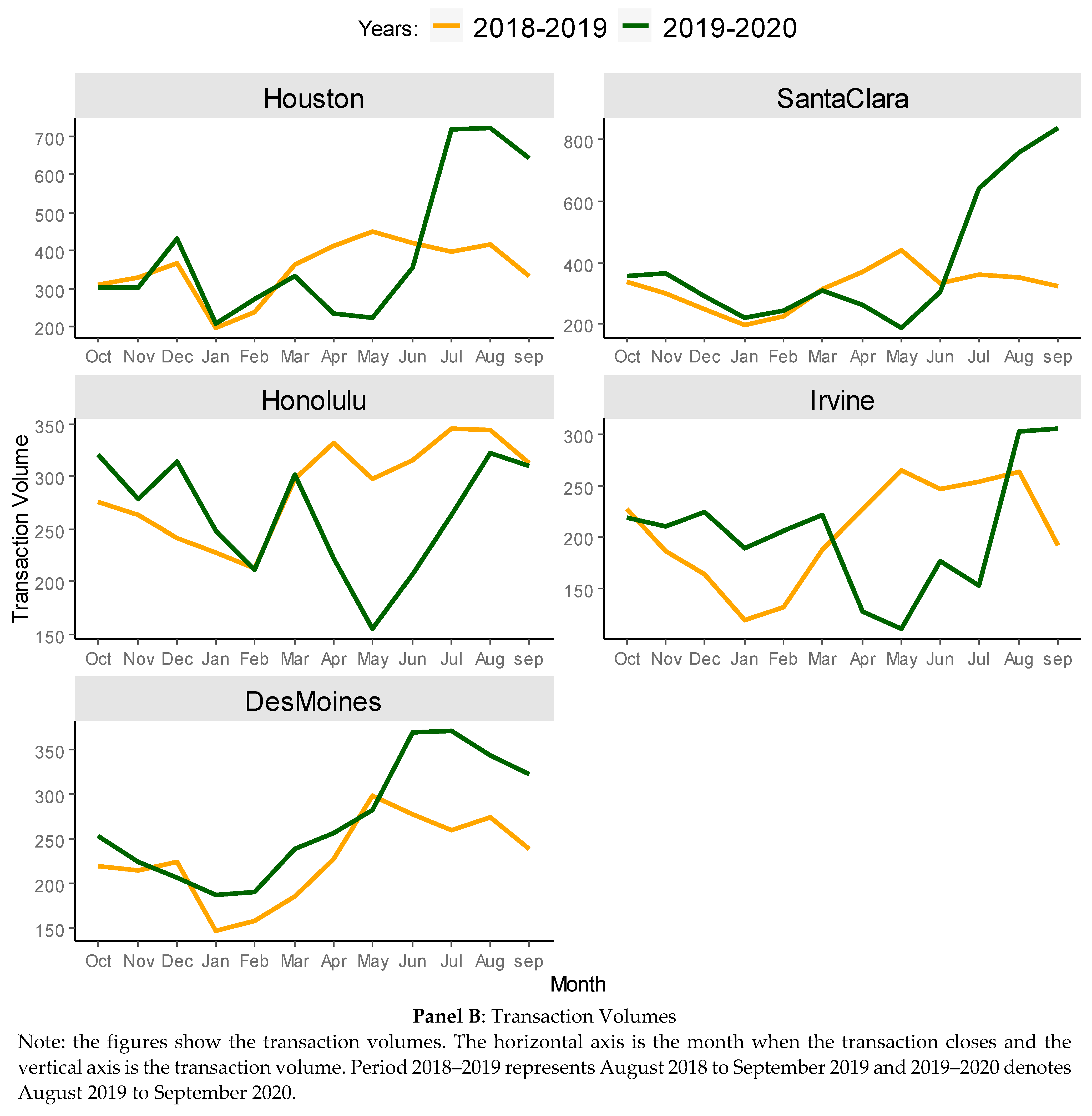
We next turn to the transaction volumes shown in Panel B of Figure 1. The changes in transaction volumes are quite similar for Houston, Honolulu, Irvine and Santa Clara. Specifically, the volume dropped after the outbreak in April and May and then increased to levels surpassing or equal to those of the previous year. It appears that the housing markets are making up for the lost transactions in April and May. For Santa Clara, the increase in transaction volumes is larger than the decrease before, suggesting that the lower interest rates might encourage more transactions. For Des Moines, the transaction volumes did not decrease but the increasing rate seemed to be disrupted in May. This is possibly due to the fact that real estate is categorized as an essential service in Iowa.

4. Results

Using the revised difference-in-differences method with non-parametric smoothing, described above, we present the COVID-19 effect on house prices for Houston, Santa Clara, Honolulu, Irvine, and Des Moines, shown in Figure 2. The horizontal axis represents February to mid-September of 2020. The transaction time from the original data dates from March to Mid-October of 2020, which specifies when the transaction closes. However, since the transaction normally takes about 30 to 45 days, we subtract 37.5 days from the original time to better represent the market conditions for when the offer is signed. To compare how the changes of house prices relate to the stay home orders, we include the start of the stay home order, the first reopening of the economy and the reverse of the reopening as three vertical lines colored purple for each of the five areas. The vertical axis shows the price impact, and an effect of 0.05 indicates that the outbreak leads to a house price increase of 5% relative to before the outbreak. The averages of the point estimates in Figure 2 are provided in

Table 3. Average Point Estimates for Figure 2.

Month of 2020	Houston	Santa Clara	Honolulu	Irvine	Des Moines
February	0.0257	0.0089	−0.0225	0.0348	0.0185
March	0.0153	0.0149	−0.0793	0.0269	0.0160
April	0.0220	0.0234	−0.0669	0.0221	0.0184
May	0.0177	0.0361	−0.0431	0.0168	0.0237
June	0.0040	0.0505	−0.0515	0.0298	0.0324
July	−0.0111	0.0655	−0.0354	0.0433	0.0404
August	0.0087	0.0789	−0.0178	0.0524	0.0320
September	0.0143	0.0997	−0.0176	0.0580	0.0201
Average	0.0121	0.0472	−0.0418	0.0355	0.0201

Note: this table provides the average point estimates for the effects in Figure 2. These are the averages of the estimates of the non-parametric estimation for each month.

.

4.1. Houston

Starting from Houston, we can see that, in February, the house price increased by about 2.5% relative to before the outbreak. The increase rate dropped slightly in March, but more or less maintained the same level in April at about 2.2%. Then, the rate started on a moderately downward trajectory and reached the trough at about −1.1% in July. Eventually, in September, the house price recovered its growing momentum. With the decreasing rate of 1.1%, for the median house price of USD 425,000—for the data included in the analyses of Houston—a net loss of USD 4675 might occur in July, relative to before. Comparing the house price effect to the timepoints of the stay home orders, there is no evidence suggesting that the orders are related to the housing market changes. Since, after the implementation of the stay home order, the housing market was on a rising trend after the stay home order ended, the increase rate of house prices was still declining.

There might be multiple reasons for this. A possible one might be that Houston is one of the cities that implemented the stay home orders relatively late in the country. The duration of the stay home order is also a litter shorter compared to other places. Thus, before the implementation of the stay home order in early April, the housing market might have already felt the negative hit from the spread, which explains the downward move before the implementation of the stay home order. After the lift of the stay home order in May, the spread actually climbed sharply4 and the economies were also still suffering from the negative shocks on employment and income, which dampens the housing market (Haurin and Gill 1987; Green and Hendershott 1995; Mayer and Somerville 2000). This explains the downward move that continues after the lift of the stay home order. Additionally, whether the stay home orders are effectively implemented is also a question. Since when we searched for restaurants in both Santa Clara and Houston in June, there was a higher portion of restaurants in Houston that still offered indoor eating when it was forbidden by the government.

4.2. Honolulu

For Honolulu, a noticeable difference in the house price change from that of Houston lies in the fact that the house price declined from February to September relative to before. Honolulu exhibits two unique features compared to the other four areas. On the one hand, it has the second lowest case rates in the US; on the other hand, it heavily depends on tourism, which is severely hit from the outbreak with travel restrictions and social distancing. The result, therefore, suggests that, even though Honolulu controlled the spread relatively better, the lack of diversity, the heavy reliance on service industries, and tourists make their housing market more vulnerable and susceptible to the negative shocks than the other four areas. This corresponds with the finding that people working in industries that require in-person contacts might experience higher income reductions (Baker et al. 2020b). Regarding the stay home orders, they do not seem to be related to house price movement either. Specifically, before the implementation of the order, the housing market had already moved out of the bottom and, after the lift of the order, there does not seem to be a significant change in the house price effects. This is reasonable, since Honolulu relies relatively more on outside forces from tourism and aviation, the effects of their local stay home orders might be limited.

4.3. Santa Clara

Formerly, the net impact from COVID-19 on house prices is generally positive for Houston, while being negative for Honolulu. It suggests that, for Houston, the positive effects from the outbreak on housing markets, such as the interest rate decrease and the inflation expectations, outweigh the negative effects from the damage on employment and income, while it is the opposite for Honolulu. However, for these two areas, the patterns of the house price effects are similar in a sense that the lines of the effects on house prices both go downward first and then regain upward momentum, while for Santa Clara, there are no downward changes in the house price effects from the figure. On the contrary, the house price increases at an exponential rate, possibly fueled by the low interest rates and skyrocketing stock prices. Thus, the result does not suggest that this area loses its attractions to homebuyers with the remote working. In contrast, the housing market fundamentals in this area seem to be fairly strong.

Regarding the effect of remote working on migration, according to the Redfin Migration data, about 77.3% of the users in the Bay Area (San Jose) still searched within the Bay area in Q3 of 2020. Only 22.7% of them were searching elsewhere. The net outflow reached 43,592 in the Bay Area in Q3 of 2020, which increases by 61.5% to the last year. In total, 25% (the highest ratio out of the leavers) of people that left the Bay Area moved to Sacramento, which is a 2 h drive from San Jose. The median house price in Sacramento was USD 387,439 in December 2020, with an increase of 11% from the previous year. Thus, indeed some people are moving out of the high-cost Bay Area to the neighboring Sacramento. Yet, the outflow did not seem to be large enough to shake the housing market of the Bay Area.

4.4. Irvine

We next turn to Irvine where the effects stay positive all the way from February to September. The increase rate of house prices in Irvine first declines slightly in May, climbs afterwards, and eventually reaches a maximum growth rate of 5.8% in September. The slight decrease in May suggests that, unlike Santa Clara, Irvine might still feel modest negative shocks, but not as many as Houston. The result subsequently indicates that low shares of residents working in service industries, better amenities of quality schools and lower crime rates might help the housing market of Irvine stay strong during these negative shocks. Additionally, the effects on house prices for Houston, Honolulu, Santa Clara and Irvine all show a rising trend in the increasing rates of house prices from July to September, suggesting the existence of a surging housing market after the outbreak. This suggests that the common factors across the areas, such as the low interest rates and the inflation expectations, might be driving these housing markets after July.

4.5. Des Moines

Finally, we turn to Des Moines where the stay home orders were not implemented but there were business restrictions that might have performed similar functions. The results specify that, first, the effect on house prices does not suggest a relationship between the business restrictions and the house price changes, similar with what we find for the stay home orders. Second, the average increase rate of house prices in Des Moines is higher than that of Houston but lower than those of Santa Clara and Irvine. As discussed before, Des Moines represents a market that might not be largely adversely influenced by COVID-19 with the low service shares and lack of stay home orders. Thus, the ranking of the effect magnitudes suggests that Santa Clara and Irvine might exhibit an extra high housing demand, while Houston might be more adversely hit compared to Des Moines.

Third, unlike the former four cities, the house price increase rate was on a declining trend in Des Moines in September. Specifically, the increase rate in Des Moines started from 1.85% in February, increased to a maximum rate of 4% in July, and ultimately fell to 2% in September. It might be that the housing markets in Houston and Honolulu are still under the stimulus from the low interest rates and recovery in economic activities, while Des Moines might have already passed the fastest growing stage. Irvine and Santa Clara, on the other hand, not only are on a rising trend in house price increase but also show increases in popularity among homebuyers. The changes in transaction volumes in Houston, Honolulu, Irvine and Santa Clara also correspond with this point. The transaction volumes reached the summit in August for Houston and Honolulu, while the maximum volume happened in September for Irvine and Santa Clara. For Des Moines, the largest transaction volume appeared in July, before the other four cities.

To sum up, the analyses suggest that the vulnerability of an area’s housing market might be related to the reliance on the service industry or other industries requiring face-to-face contact, which are severely influenced by the spread. A more diverse economy, a lower share of residents working in services industries and better amenities seem to be associated with more positive house price movements. There is no evidence suggesting that the stay home orders, or business restrictions, are related to house price changes.

5. Conclusions

In this article, we explore the effect of COVID-19 on house prices. Specifically, we self-collected individual property transaction data for five areas of Houston, Santa Clara, Honolulu, Irvine and Des Moines. These areas vary in the shares of service industries, the housing market fundamentals, and the start- and end-time of stay home orders. Employing a revised difference-in-differences method with non-parametric smoothing that controls more vigorously for the unobservables, we are able to model the effects of the outbreak on house prices as a continuous function of time. We then compare the effects across these five areas and analyze how the effects might be related to the stay home orders.

The results show that, after the outbreak, Honolulu is the only place that experienced declines in house prices with the largest decrease rate approaching 6.69% in April 2020. For the other four areas, which see increases in house prices, the largest increase rate of 9.97% appears in Santa Clara followed by Irvine with a growth rate of 5.80%. Houston and Des Moines also generally experienced increases in house prices. There exists no evidence suggesting that the COVID-19 effects on house prices are related to the stay home orders or the business restrictions. Therefore, the results indicate that a housing market might be put in a vulnerable position from the outbreak if the local economy relies heavily on tourism, service and aviation, which require face-to-face interactions. The historically low interest rates might fuel rapid growth in areas with strong housing market fundamentals and better amenities. The vulnerable areas can benefit from government subsidies to make up for the loss and to prevent future damages. For investors, it might be wise to avoid entering the housing market at the highest point. One limitation from the analyses is that, during the time of the research, COVID-19 was still spreading and we are unsure how the situation is about to evolve in the near future, which may bring differential effects on the housing markets.

References

- Baker, Scott R, Nicholas Bloom, Steven J Davis, Kyle Kost, Marco Sammon, and Tasaneeya Viratyosin. 2020a. The Unprecedented Stock Market Reaction to COVID-19. The Review of Asset Pricing Studies, raaa008. [Google Scholar]
- Baker, Scott R, Robert A. Farrokhnia, Steffen Meyer, Michaela Pagel, and Constantine Yannelis. 2020b. How Does Household Spending Respond to an Epidemic? Consumption during the 2020 COVID-19 Pandemic. The Review of Asset Pricing Studies 10: 834–62. [Google Scholar] [CrossRef]
- Brueckner, Jan K., and James R. Follain. 1989. ARMs and the demand for housing. Regional Science and Urban Economics 19: 163–87. [Google Scholar] [CrossRef]
- Campbell, John Y., Stefano Giglio, and Parag Pathak. 2011. Forced Sales and House Prices. American Economic Review 101: 2108–31. [Google Scholar] [CrossRef] [Green Version]
- CNBC. 2020. 5 Charts Show What the Global Economy Looks Like Heading into 2021. Available online: https://www.cnbc.com/2020/12/28/5-charts-show-covid-impact-on-the-global-economy-in-2020.html (accessed on 14 January 2021).
- CNN. 2020. Federal Reserve Cuts Rates to Zero to Support the Economy during the Coronavirus Pandemic. Available online: https://edition.cnn.com/2020/03/15/economy/federal-reserve/index.html (accessed on 14 January 2021).
- Del Giudice, Vincenzo, Pierfrancesco De Paola, and Francesco Paolo Del Giudice. 2020. COVID-19 Infects Real Estate Markets: Short and Mid-Run Effects on Housing Prices in Campania Region (Italy). Social Sciences 9: 114. [Google Scholar] [CrossRef]
- Diamond, Rebecca, and Timothy McQuade. 2019. Who Wants Affordable Housing in their Backyard? An Equilibrium Analysis of Low Income Property Development. Journal of Political Economy 127: 1063–17. [Google Scholar] [CrossRef] [Green Version]
- Green, Richard K., and Patric H. Hendershott. 1995. Age, Housing Demand, and Real House Prices. Regional Science and Urban Economics 26: 465–80. [Google Scholar] [CrossRef]
- Harris, J.C. 1989. The effect of real rates of interest on housing prices. The Journal of Real Estate Finance and Economics 2: 47–60. [Google Scholar] [CrossRef]
- Haurin, Donald R., and H. Leroy Gill. 1987. Effects of income variability on the demand for owner-occupied housing. Journal of Urban Economics 22: 136–50. [Google Scholar] [CrossRef]
- Ling, David C., Chongyu Wang, and Tingyu Zhou. 2020. A First Look at the Impact of COVID-19 on Commercial Real Estate Prices: Asset-Level Evidence. Review of Asset Pricing Studies. Available online: https://ssrn.com/abstract=3593101 (accessed on 23 June 2020). [CrossRef]
- Loxton, Mary, Robert Truskett, Brigitte Scarf, Laura Sindone, George Baldry, and Yinong Zhao. 2020. Consumer Behaviour during Crises: Preliminary Research on How Coronavirus Has Manifested Consumer Panic Buying, Herd Mentality, Changing Discretionary Spending and the Role of the Media in Influencing Behaviour. Journal of Risk and Financial Management 13: 166. [Google Scholar] [CrossRef]
- Mayer, Christopher J., and C. Tsuriel Somerville. 2000. Residential Construction: Using the Urban Growth Model to Estimate Housing Supply. Journal of Urban Economics 48: 85–109. [Google Scholar] [CrossRef] [Green Version]
- Mazur, Mieszko, Man Dang, and Miguel Vega. 2020. COVID-19 and the march 2020 stock market crash. Evidence from S&P1500. Finance Research Letters, 101690. [Google Scholar] [CrossRef]
- Mian, Atif, and Amir Sufi. 2011. House Prices, Home Equity-Based Borrowing, and the US Household Leverage Crisis. American Economic Review 101: 2132–56. [Google Scholar] [CrossRef] [Green Version]
- NBC. 2020. Will a Work From Home Exodus Drop Bay Area Housing Prices? Available online: https://www.nbcbayarea.com/news/coronavirus/will-a-work-from-home-exodus-drop-bay-area-housing-prices/2295371/ (accessed on 14 January 2021).
- Schwab, Robert M. 1982. Inflation Expectations and the Demand for Housing. American Economic Review 72: 143–53. [Google Scholar]
- Shilling, James, John Benjamin, and C. Sirmans. 1990. Estimating Net Realizable Value for Distressed Real Estate. Journal of Real Estate Research 5: 129–40. [Google Scholar]
- Thatcher, Arran, Mona Zhang, Hayden Todoroski, Anthony Chau, Joanna Wang, and Gang Liang. 2020. Predicting the Impact of COVID-19 on Australian Universities. Journal of Risk and Financial Management 13: 188. [Google Scholar] [CrossRef]
- Thorbecke, Willem. 2020. The Impact of the COVID-19 Pandemic on the U.S. Economy: Evidence from the Stock Market. Journal of Risk and Financial Management 13: 233. [Google Scholar] [CrossRef]
- Viscusi, W. 1990. Sources of Inconsistency in Societal Responses to Health Risks. The American Economic Review 80: 257–61. [Google Scholar]
- Wang, Chuanyi, Zhe Cheng, Xiao-Guang Yue, and Michael McAleer. 2020. Risk management of COVID-19 by universities in China. Journal of Risk and Financial Management 13: 36. [Google Scholar] [CrossRef] [Green Version]
- Wong, Grace. 2008. Has SARS infected the property market Evidence from Hong Kong. Journal of Urban Economics 63: 74–95. [Google Scholar] [CrossRef] [PubMed]
- Yue, Xiao-Guang, Xue-Feng Shao, Rita Yi Man Li, M. James C. Crabbe, Lili Mi, Siyan Hu, Julien S Baker, Liting Liu, and Kechen Dong. 2020. Risk Prediction and Assessment: Duration, Infections, and Death Toll of the COVID-19 and Its Impact on China’s Economy. Journal of Risk and Financial Management 13: 66. [Google Scholar] [CrossRef] [Green Version]