
Bitcoin and Portfolio Diversification: A Portfolio Optimization Approach


1
School of Business, Western Sydney University, Sydney 2751, Australia
2
College of Business Administration, American University of the Middle East, Eqaila 54200, Kuwait
*
Author to whom correspondence should be addressed.
†
Current address: Locked Bag 1797, Penrith 2751, Australia.
J. Risk Financial Manag. 2021, 14(7), 282; https://doi.org/10.3390/jrfm14070282
Submission received: 7 May 2021
/
Revised: 12 June 2021
/
Accepted: 17 June 2021
/
Published: 22 June 2021
(This article belongs to the Special Issue Advanced Portfolio Optimization and Management)
Abstract
:This study investigates the performance of Bitcoin as a diversifier under different constraining portfolio optimization frameworks. The study employs different constraining optimization frameworks that seek to maximize risk-adjusted returns (Sharpe ratio) of the portfolio by optimizing allocations to each asset class (asset allocation). The performance attributes are evaluated by comparing the portfolios both with and without Bitcoin under frameworks ranging from equal-weighted, risk-parity, and semi-constrained to unconstrained. This study suggests that Bitcoin, due to its exotic nature, unwavering appeal, and unknown set of drivers, could act as a diversifier in normal market conditions, and it might also have some borderline hedge to safe haven properties. The results further suggest that while Bitcoin may be a potential diversifier for a risk-seeking investor, the risk-averse investor must exercise caution by limiting their exposure to Bitcoin in their portfolios, as unnecessary exposure may increase the probability of losses in extreme market conditions.
JEL Classification:
G11; G15; C581. Introduction
One of the very disruptive and significant developments post-global financial crisis (GFC) has been the emergence of cryptocurrencies, Bitcoin in particular. Bitcoin is a decentralized, peer-to-peer electronic cash system designed by Satoshi Nakamoto (a pseudonym) in 2008 that does not rely upon a trusted third-party or any central authority but uses cryptography for transfers, control, and management (Nakamoto 2008). The global financial crisis (GFC) during 2008–2009 was classified as a period of severe distress to most economies across the globe, the effects of which ranged from higher inflation, growing budget and trade deficits, currency devaluations, and dwindling currency reserves. As the GFC unfolded, investors discovered that they were less diversified than they originally thought they were and therefore started looking for alternative investments that might be considered safe havens, hedges, or diversifiers. It was in this context that Bitcoin rose to prominence; by April 2018, Bitcoin (BTC) had a total market capitalization of more than USD 116 billion (Yi et al. 2018), which rose to almost USD 700 billion by May 2021.1 Nakamoto (2008) argued that due to its high transaction cost and the exclusion of a substantial portion of the world population from the formal financial system, fiat money is no longer a proper medium of exchange. Therefore, by making BTC supply predetermined, it has the potential to serve as a proper medium of transaction that is insulated against inflation and as a reliable store of value (driven by precautionary motives) in the long run.
Cryptocurrencies, in general, have evolved by gradually shifting from being an immature market to almost reaching maturity over the last decade. Wątorek et al. (2021) attributed this development to the growth of new trading platforms and exchanges as well as to a substantial increase in trading volumes and frequency. They also argued that although the exchange rates for most liquid cryptocurrency pairs resembled those of the forex markets, developments in the cryptocurrency markets were still quite distinct from the forex markets in terms of varying liquidity, different trading platforms, and the existence of marginal arbitrage opportunities for less-liquid cryptocurrency pairs. While the cryptocurrency market is still evolving and has yet to attain complete maturity, it would be amiss to say that its popularity and acceptance are not gaining momentum within the financial mainstream. Despite a huge leap in the acceptance of Bitcoin as a medium of exchange, it has nonetheless failed to gain momentum in retail transactions, particularly due to its exotic nature and its anti-regulatory, anti-environment, and fraudulent ‘feel’. Moreover, Bitcoin has also failed to establish itself as an alternative asset, as it is believed that the Bitcoin market is far from efficient due to the huge interest of young, inexperienced individual investors and the subsequent absence of institutional investors and lack of enough taxation and regulatory regulations by most countries (Tan and Low 2017; Bouri et al. 2019). Opinions about the nature and characteristics of Bitcoin vary across a wide spectrum; while some consider it an alternative to official fiat money and a step toward the development of digital currencies (Bouri et al. 2017b), a large number of researchers and practitioners consider Bitcoin simply another speculative asset (Glaser et al. 2014; Baek and Elbeck 2015; Williamson 2018). On the other hand, some researchers have likened Bitcoin to gold, often referring to it as ‘digital gold’ (Selmi et al. 2018), while Bouri et al. (2017a) considered Bitcoin a positive disruption and viewed it as an alternative to official fiat currency.
Recent developments in the global financial and economic landscape have allowed Bitcoin to gain some ground in terms of acceptance as a medium of transaction, but mostly as an alternative asset that provides a hedge against domestic economic troubles and imprudent monetary policy actions. Amid the ongoing uncertainties regarding conventional financial systems and the economic troubles faced by many countries, Bitcoin has gained some ground in its popularity and ‘feel’ (Bouri et al. 2017a). Dyhrberg (2016a) believed that global uncertainties in the wake of the global financial crisis abetted in and strengthened the positive outlook and popularity of Bitcoin. Bitcoin, as it is often compared to gold and exhibits some safe haven properties, has also gained prominence due to a loss of faith in the stability of the conventional financial architecture. This is evident from the chaos created by the much-hyped and politically motivated demonetization experiment enforced by the Indian government and the Venezuelan government, restricting transaction limits and the movement of capital in addition to hampering informal business operations (Bouoiyour and Selmi 2017). The fact that Bitcoin is neither subject to a country’s political and economic misadventures nor depends upon a central authority that could restrict the movement of capital has led to the emergence of the notion that Bitcoin may provide substantial diversification, hedge, and safe haven benefits in addition to being an effective medium of transaction.
Since its inception, Bitcoin has attracted a lot of interest from the academic community and practitioners alike. While the existing research has largely focused on the technological and legal aspects of Bitcoin, scholars have recently taken up investigating the financial and economic aspects of Bitcoin as well, particularly regarding its potential in portfolio diversification. The fundamental objective of portfolio diversification is to construct a portfolio of uncorrelated or mildly correlated assets to maximize risk-adjusted returns on investment. Portfolio optimization is one of the techniques used by investment professionals to explore the potential of different assets in maximizing the risk-adjusted returns of the portfolio by adjusting the weight of each asset using either simulations or constrained scenarios. A significant amount of research has already been conducted in the area of portfolio diversification, which helps investors devise their investment strategies and policies. Lately, cryptocurrencies in general and Bitcoin in particular have aroused significant interest among investment professionals, policymakers, and regulators alike. Although much research has primarily focused on the legal and technological aspects of Bitcoin, the examination of other financial, diversification, hedge, and safe haven aspects of Bitcoin has not progressed as far. To this end, the present study explores the potential of Bitcoin in portfolio diversification using a portfolio optimization approach as well as establishing the alternative asset characteristics (or otherwise) of Bitcoin.
The empirical literature on the nature of linkages between gold and other assets and subsequently, the potential of gold as a diversifier, a hedge, or a safe haven has grown remarkably. A vast literature discussing the different diversification-to-safe haven properties of gold has been well established (Ciner 2001; Kaul and Sapp 2006; Miyazaki and Hamori 2014; Ciner et al. 2013; Reboredo 2013; Beckmann et al. 2015). Bitcoin, likewise, demonstrates properties similar to gold in many ways; research has suggested that due to the unique risk–return characteristics of Bitcoin and its uncorrelated nature with other assets, Bitcoin might as well serve as a safe haven against global financial stress, commodities, and energy (Bouri et al. 2017a, 2017c, 2018) as well as a hedge against equities, currencies, commodities, and VIX (Bouri et al. 2017b, 2017c; Chan et al. 2019; Dyhrberg 2016a; Baur et al. 2018).
This study is one of the very few studies exploring the diversification potential of Bitcoin using a portfolio optimization approach. Earlier studies using a portfolio optimization approach can be classified into four categories: The first category includes studies that focus on portfolio optimization in general, Bitcoin not being a component of such frameworks (Ehrgott et al. 2004; Krokhmal et al. 2002; Cai et al. 2000; DeMiguel et al. 2009; Gaivoronski and Pflug 2005); the second category of studies have either focused on the US markets (Brière et al. 2015; Carrick 2016; Wu and Pandey 2014) or local markets (Aggarwal et al. 2018; Gangwal 2017; Kajtazi and Moro 2017); another strand of literature has generally addressed cryptocurrencies and digital currencies (Boiko et al. 2021; Colombo et al. 2021; Wang and Ngene 2020; Ma et al. 2020), and the fourth category of studies have evaluated the diversification potential of Bitcoin with limited indices, assets, or variables (Platanakis and Urquhart 2020; Garcia-Jorcano and Benito 2020; Pal and Mitra 2019; Eisl et al. 2015). The current study contributes to the existing literature by using a wide range of variables with the most recent data, thus bringing in new evidence regarding the potential for Bitcoin in portfolio diversification using a portfolio optimization approach.
2. Literature Review
The literature on cryptocurrencies has evolved rapidly as they have gained prominence and the attention of researchers amidst the ongoing economic and financial downturn. Significant interest is also evolving among researchers wanting to learn how the characteristics, price development, and volatility of cryptocurrencies and Bitcoin, in particular, will evolve through the current downturn in financial markets. Dwyer (2015) investigated the return volatility of Bitcoin and found that, on average, it was higher than other assets such as gold. Blau (2017) conducted a dynamic analysis of Bitcoin price fluctuations and concluded that the unusual volatility in Bitcoin prices was due mainly to speculation. Several other studies have also explored the price determinants of cryptocurrencies (Brauneis and Mestel 2018; Ciaian et al. 2016; Garcia et al. 2014; Kristoufek 2015; Cheah and Fry 2015). For instance, Ciaian et al. (2016) found that Bitcoin prices were mainly attributed to the supply and demand generated mostly by investors departing from rationality (Bouri et al. 2019). Similarly, Kristoufek (2015) and Garcia et al. (2014) confirmed the role of increased public attention and Google trends in the development of Bitcoin prices. Kristoufek (2015) also argued that Bitcoin markets were weakly related to stock markets due to different underlying price determinants. Another strand of literature has investigated the financial maturity of Bitcoin including the work of Wątorek et al. (2021), Dyhrberg et al. (2018), Koutmos (2018), and Nadarajah and Chu (2017). It is argued in these studies that the cryptocurrency market, and Bitcoin in particular, have reached a considerable level of maturity and can be considered an alternative investment. With regard to liquidity and investability, only a few academics have explored cryptocurrencies’ liquidity and investability (Wątorek et al. 2021; Dyhrberg et al. 2018; Karalevicius et al. 2018; Wei 2018).
Boiko et al. (2021) and Wang and Ngene (2020) argued that while the inclusion of different cryptocurrencies in a diversified portfolio under different portfolio optimization strategies could lead to substantial enhancements in portfolio performance, Bitcoin was still a dominant force in the cryptocurrency portfolio. Ma et al. (2020), on the other hand, argued that the addition of multiple cryptocurrencies could lead to better portfolio performance; however, Ethereum offered better diversification potential than Bitcoin. From the standpoint of volatility spillover, Burnie (2018) and Guesmi et al. (2019) found that the inclusion of Bitcoin could enhance portfolio diversification due to the lack of noticeable spillover effects between Bitcoin and other financial assets. Conrad et al. (2018) showed that the realized volatility of Bitcoin was negatively correlated with other assets, and that the riskiness in US markets was negatively related to Bitcoin volatility. They also showed that the volatility in Bitcoin decreased during financial distress or flight-to-safety periods, thereby demonstrating the ability of Bitcoin to offer potential in portfolio diversification. Wątorek et al. (2021) found that the most liquid cryptocurrencies, e.g., BTC and ETH, were uncorrelated to traditional financial instruments, on average, and therefore might facilitate portfolio diversification. Ozturk (2020) suggested that Bitcoin might not provide sufficient contributions to portfolio diversification in the short and medium term, particularly due to the volatile nature of Bitcoin; however, due to limited connectedness between Bitcoin and other assets in the long run (gold and crude oil), it might offer potential gains from diversification in the long run. Platanakis and Urquhart (2020) reported that Bitcoin might generate substantial, risk-adjusted portfolio returns in a diversified stock–bond portfolio under various asset allocation strategies considering different levels of risk tolerance. Bouri et al. (2020) strongly supported Bitcoin as a potential diversification asset, with its benefits surpassing that of gold and commodities. They also reported that Bitcoin resembled gold in its safe haven properties and was, in fact, a superior safe haven for stocks over gold and commodities. Shahzad et al. (2019), on the other hand, showed that Bitcoin had the highest risk-return Sharpe ratio in contrast to gold, which had a much lower Sharpe ratio. They found that although Bitcoin and gold had similar characteristics, gold was associated with very few extreme losses compared to Bitcoin. Their results also revealed that Bitcoin could at best offer potential for a weak safe haven similar to gold and commodities, but not for all markets under study. They attributed the weak safe haven nature of Bitcoin to a difference in the underlying determinants of price evolution in the two markets as well as the differences in the pools of investors in the two markets. Pho et al. (2021) found that while Bitcoin might act as a potential diversifier for risk-seeking investors, gold continued to be a superior diversifier for risk-averse investors. Jeribi and Fakhfekh (2021) argued that the contribution of Bitcoin to portfolio diversification might not be as substantial as generally argued; their results suggested that to maximize risk-adjusted return, investors must hold a larger proportion of conventional assets in their portfolio with a very small exposure in cryptocurrencies. Similar results were reported by Bouri et al. (2019), Kristoufek (2015), and Bouoiyour et al. (2016). Conrad et al. (2018), on the other hand, indicated that the behavior of Bitcoin was considerably different than gold during high volatility periods, and thus the comparisons to gold as a safe haven were questionable to some degree. Wątorek et al. (2021) found that while the cryptocurrency market showed no cross-correlation with traditional assets until recently, this relationship shifted during the COVID-19 crisis, thereby undermining the potential of cryptocurrencies (BTC and ETH being the most liquid) as safe havens.
Pal and Mitra (2019) showed that Bitcoin could provide a hedge against equity markets, gold, and commodities. They also indicated that the hedging effectiveness of Bitcoin was highest with gold; a long position in Bitcoin provided a hedge with a short position in gold. Garcia-Jorcano and Benito (2020) found strong evidence in support of Bitcoin in portfolio diversification; they also reported that Bitcoin might act as a hedge against all international stock markets in normal market conditions, although such potential was found to be stronger for the Hong Kong and Shanghai markets. Moreover, it was also reported that during extreme market conditions, Bitcoin might fail to hedge the risk in stock markets, though still acting as a diversifier. On the other hand, Baur et al. (2018) tested the hedging capabilities of Bitcoin as compared to foreign exchange markets and stock markets throughout different periods in a dynamic framework. They concluded that Bitcoin should be considered a speculative asset rather than a transaction medium. Ji et al. (2018) tested the potential influence of changes in different assets’ prices on Bitcoin and affirmed the idiosyncratic price movements of Bitcoin. More recently, Khaki et al. (2020) found that the value of Bitcoin was not closely correlated with capital markets or the forex market. The uncorrelated nature of Bitcoin with other conventional assets might indicate a potential diversification benefit when added to a well-diversified portfolio. Mazanec (2021) argued that Bitcoin was leading the way for altcoins such as Binance Coin, Cardano, Litecoin, and Ethereum to either replace or somehow supplement it as a potential asset for portfolio diversification. To sum up, the majority of research has confirmed the lack of interaction and spillover effects among Bitcoin and different groups of financial assets. This, in turn, raises the question as to whether an optimal mix of Bitcoin and other assets could enhance the risk–return tradeoff of a well-diversified portfolio and if so, what implications this might have for investors’ investment strategies.
Research using the portfolio optimization approach has also attempted to gauge the efficacy of adding Bitcoin to different portfolio frameworks including well-diversified portfolios. Empirical evidence on the potential benefits of adding Bitcoin to a well-diversified set of portfolios was provided by Brière et al. (2015). They employed the mean-variance tests of Kandel and Stambaugh (1987) and Ferson et al. (2013) to investigate the impact of Bitcoin inclusion on the risk–return trade-offs of three dissimilar, well-diversified portfolio frameworks. They reported that the inclusion of Bitcoin in a well-diversified portfolio, even in a small proportion, yielded superior mean-variance tradeoffs as compared to Bitcoin-free portfolios. Similarly, Brière et al. (2015) and Eisl et al. (2015) utilized the conditional value-at-risk approach to the four most widely used portfolio frameworks and provided further evidence on the role of Bitcoin in enhancing expected returns as well as the levels of risk of proposed portfolios; however, they claimed that Bitcoin’s contribution in leveraging expected returns overweighed the additional risk. These results were supported by Gangwal (2017), who analyzed the effect of adding Bitcoin to a well-diversified portfolio under various minimum holding constraints and including various asset classes. He found that adding Bitcoin almost always improved the portfolio’s risk-adjusted return as measured by the Sharpe ratio, especially when unconstrained short selling was allowed. In a similar study, Symitsi and Chalvatzis (2019) employed daily data on multiple exchange rates, gold, oil prices, and a pool of stocks to measure Bitcoin performance in different optimized portfolios under different constraining scenarios. Their results confirmed the role of Bitcoin in enhancing the Sharpe ratio with no statistically significant increase in portfolios’ variances, especially for equally weighted and global optimal minimum variance portfolio strategies.
Bitcoin has also spurred interest in its potential contribution to portfolio diversification and risk hedging. Bouri et al. (2017a) found that Bitcoin could be considered a good hedge, as its prices tended to move against commodities prices. Similarly, Baumöhl (2019) affirmed the importance of Bitcoin in portfolio diversification, as it exhibited a low correlation with a variety of asset classes. Aggarwal et al. (2018) found that Bitcoin offered superior, risk-adjusted return performance of portfolios under naïve and long-only frameworks across the investment horizon as compared to a constrained portfolio framework. DeMiguel et al. (2009) reported similar results and showed that the performance of a naïve portfolio specification was as good as other constraining scenarios or sometimes even better. Brière et al. (2015) showed that by adding Bitcoin to an already diversified portfolio of US assets, the Sharpe ratio (Sharpe 1963) improved. Other studies have used other risk–return measures such as the Omega ratio (Wu and Pandey 2014), value at risk (VaR), and conditional value at risk (CVaR) (Eisl et al. 2015; Aggarwal et al. 2018; Selmi et al. 2018) to evaluate the effectiveness of Bitcoin in portfolio diversification through optimization. More recent research has provided further support, arguing that an optimal mix of Bitcoin and US equities could reduce the overall risk of a portfolio (Bouri et al. 2017a). Interestingly, similar results were obtained in portfolios that included foreign currencies, commodities, stocks, and ETF (Andrianto and Diputra 2017) as well as portfolios including global and emerging market indices (Guesmi et al. 2019). In addition, more recently, Kajtazi and Moro (2019) evaluated the impact of Bitcoin on portfolio optimization and diversification in the context of US, European, and Chinese investors by adding Bitcoin to four different portfolio scenarios—naïve, long-only, unconstrained, and semi-constrained. They reported that Bitcoin improved the return but increased the riskiness of the portfolios, correspondingly.
To sum up, a survey of the literature reveals that there is no established consensus on whether Bitcoin can serve investors as a portfolio diversifier, a hedge, or a safe haven. The lack of consensus can be attributed to numerous factors including different methodologies, sample periods, and posited determinants. For greater clarity, and perhaps consensus, to emerge about the appropriate role, if any, that Bitcoin should or could play in portfolio management, further empirical research is required. This paper thus contributes to that knowledge goal by employing a little-used approach to the investigation of the potential effectiveness of Bitcoin in portfolio diversification—namely, a portfolio optimization approach under multiple constraining scenarios.
3. Data Description and Research Methodology
This study aims to evaluate the diversification potential of Bitcoin in a well-diversified portfolio by employing portfolio optimization approach and Monte Carlo simulation. Herein, the focus is on the empirical risk measures and risk-adjusted return measures derived from historical data without approximating for an efficient frontier or a portfolio represented by historical VaR. A Monte Carlo simulation was employed to compute the VaR at 95% and 99%, with 10,000 iterations for each portfolio framework described in the following section. The historical VaR was also computed to compare against the variance–covariance VaR and Monte Carlo simulated VaR to compare historical, covariance-based, and expected (normalized) VaR and to present a decent contrast and comparison of multiple portfolios under different constrained scenarios. In addition to VaR, conditional VaR for each alternative was estimated at 95% and 99% confidence intervals to account for extreme market conditions. Under each constraining scenario, the analysis comprised two portfolios, one with Bitcoin and the other without Bitcoin.
The portfolio for the optimization comprised broad market indices for equity, currency, global economic activity, energy, fixed-income (corporate bonds), and a commodity (gold). The description of the variables is presented in Table 1 below. The following proxies were employed in this study; S & P 500 for equity markets (SBB/USD), USD to Euro (USD/WCBN) for Forex markets, the Baltic Dry Index (BALTICF) for real economic activity, the Dow Jones UBS Energy Spot Subindex (DJUBENS) for energy markets, the iShares Long-Term Corporate Bond ETF (U:IGLB) for corporate bonds, and the CMX-Gold 100 ounce (NGCC.01) for gold. This study attempted to explore the diversification potential of Bitcoin, as it still possessed a dominant power in the cryptocurrency market despite the exponential rise of cryptocurrencies in recent times. As reported by Wang and Ngene (2020), despite the phenomenal prominence of altcoins in recent times, Bitcoin still exhibited a leading and dominant role in price discovery and volatility transmission throughout the cryptocurrency market and therefore, studying the dynamics and interaction of Bitcoin with other asset classes became imperative to portfolio diversification, hedging, and understanding the origins and drivers of price and volatility in the cryptocurrency market. Moreover, as of May 2021, Bitcoin market capitalization was close to US $700 billion, which was almost 45% of the total cryptocurrency ecosystem with more than 10,000 cryptocurrencies trading on around 380 exchanges.2 The data for all the selected asset classes (or indices) was downloaded from the Thomson Reuters Eikon DataStream with weekly frequency and time-stamped from August 2011 to May 2021, with a total of 508 observations for each variable. The study employed weekly data instead of daily data, particularly because the reported variables (assets) had different market establishment and trading timelines, especially with regard to operating days and hours. Therefore, the data was employed using a weekly frequency to get consistent, balanced, and non-missing data consistent with the approach suggested by Chung and Liu (1994), Click and Plummer (2005), DeFusco et al. (1996), and Nguyen and Huynh (2019). Moreover, the monthly data did not provide qualitative data for robust evaluation, while the daily data captured too much noise and involved high transaction costs when it came to portfolio rebalancing strategies (Platanakis and Urquhart 2019). It was also found that portfolio performance increased as the rebalancing frequency increased from a daily to a weekly or bi-weekly frequency, while monthly or longer rebalancing frequencies might have caused a substantial decline in portfolio performance (Pooter et al. 2008). It was, therefore, prudent to use weekly data in the portfolio optimization scenario to gather meaningful insights compared to daily or monthly data. A number of studies based on portfolio optimization framework have employed weekly data, owing to the reasons cited above (Deng et al. 2012; Mendes et al. 2016; Ivanova and Dospatliev 2017).
The variables of the study are listed in the table below:
The mean-variance approach was used to determine the optimal weights of assets/indices under multiple constraining scenarios. The mean-variance optimization approach is described below.
3.1. Mean-Variance Optimization
Markowitz (1952, 1958) proposed a classical approach to portfolio optimization based on the conflicting criteria of maximizing the expected return and minimizing portfolio risk represented by their variance. This approach came to be known as the Markowitz covariance model, or the mean-variance approach in general. This model is formulated below:
where is the number of assets in a portfolio; denotes the fraction of investment in each asset denotes the expected return of asset ; is the covariance between the returns of assets ; and as the n-dimensional solution vector.
Consider a finite set of financial assets/indices/variables . These assets generate returns within a given observation period as below:
where is a random variable with finite means, measured as the relative increase (or decrease) in asset prices during the period under consideration. Within a budget constraint of 1, the investor may decide on the positions
in those arbitrary assets chosen by the investor within the different constraining scenarios and a budget constraint . Let be the vector of ones, and the budget constraint may be denoted by . The portfolio return at the end of the observation period is calculated as
Assuming R is a random variable, the expected return and the standard deviation of the portfolio is
where is the covariance between the returns of individual assets based on the historical observations captured by , the covariance matrix ().
Suppose is a risk measure such as variance or standard deviation. While multiple measures of risk-adjusted performance could be used, Gaivoronski and Pflug (2005) argued that in addition to conventional measures of risk such as standard deviation, some investors expressed their risk preference in terms of VaR. Therefore, for a specific risk measure for a given minimum expected return τ, the solution of the general optimization problem is given by:
where (under a short-selling constrained portfolio or as defined under each constraining scenario).
Let ω represent the vector of security weights, and is the covariance–variance matrix of the security/index returns and μ a vector of expected returns. For the same risk measure above and the expected Sharpe ratio for each asset, the solution to the maximum Sharpe ratio optimization problem is given by
where for a long-only constrained portfolio, is unbounded in case of a non-constrained portfolio, or is as described under different constraining frameworks, and is the risk-free rate. The proposition described by Jagannathan and Ma (2003) for a constrained portfolio for , the optimization solution to 1-norm-constrained mean-variance, is the same as that of the short-sale-constrained mean-variance portfolio.
The current study evaluates the diversification potential of Bitcoin in a well-diversified portfolio, using a portfolio optimization approach and a Monte Carlo simulation. The indices or variables used in the portfolio optimization process comprised broad indices for equity, currency, fixed-income, commodities, energy, and global economic activity as described in the previous section. The basic aim behind this approach was to calculate optimal weights of each asset under each constraining scenario for a well-diversified portfolio without Bitcoin and then to explore the effects of adding Bitcoin by comparing the risk–return metrics of the optimized portfolios. Each optimal portfolio, therefore, repeated the weight optimization process under the different user-defined portfolio optimization frameworks described below. The portfolio frameworks developed from an equal-weighted portfolio with and without Bitcoin by adding multiple constraining scenarios to find the optimized solution under each. The optimization was based entirely on maximizing the Sharpe ratio as described above (except for the risk parity portfolios, where the objective of the optimization was parity in the risk contribution of each asset), where the risk-free rate was assumed to be zero. Each portfolio-constraining scenario (or otherwise) can be described as follows:
3.1.1. Scenario 1: Equal-Weighted or Naïve Portfolio ()
The equal-weighted or naïve portfolio comprised all assets with equal weights, irrespective of their risk–return and covariance–variance characteristics. Researchers have shown that a naïve portfolio performs as well as a mean-variance-based optimization portfolio. Therefore, it was interesting to evaluate whether adding Bitcoin to a well-diversified portfolio under the naïve scenario could increase the risk-adjusted, mean-variance-based performance of the portfolio.
3.1.2. Scenario 2: Semi-Constrained Max-Long Portfolio (
Here, the optimization process limited the maximum position of any asset to 25 percent of the total portfolio, with no constraints on shorting. The constraint of maximum position weight limited the unreasonable or disproportionately large allocations from the unconstrained scenario. It was, thus, interesting to discover how adding Bitcoin to user-determined weight constraints could enhance the risk-adjusted, mean-variance based performance of a diversified portfolio.
3.1.3. Scenario 3: Semi-Constrained Min-Long Portfolio (
This scenario was also created to limit the unreasonable or disproportionately large allocations in the unconstrained or semi-constrained portfolio optimization problem described by Eisl et al. (2015). This framework employed a 10 percent minimum long constraint with no shorting constraint on the weight of individual assets to ensure that the portfolio was well-diversified and had a feasible optimization solution.
3.1.4. Scenario 4: Constrained Portfolio 1 (
Here, the framework sought to maximize the risk-adjusted return of the portfolio by adding a constraint in either direction that was different from the constraints employed by Eisl et al. (2015). This framework was interesting for determining the theoretical solution to an optimization problem while allowing for maximum weight in each asset to be 25 percent of the portfolio in either long or short positions. Knowing that shorting might not be possible in many assets due to the unavailability of suitable financial products, this framework helped us understand the potential of adding an asset to a well-diversified portfolio if shorting was possible.
3.1.5. Scenario 5: Risk Parity (Long Only) Portfolio (
In the risk parity portfolio optimization approach, the main objective was to have an equal contribution to the portfolio risk from each asset or asset class in the portfolio (Lee 2011). The purpose of this strategy was to limit the disproportionate economic or financial impact of a single asset on the portfolio (Ngene et al. 2018). This strategy was a very effective approach to diversification and included asset classes with high volatilities in the portfolio. In this scenario, the optimization strategy sought to maximize the risk-adjusted return of the portfolio by adding the constraint that the risk contribution of each asset to the total risk of the portfolio should be equal. The framework employed a no-shorting constraint on the weight of the individual assets as was usually the practice in a risk parity portfolio.
3.1.6. Scenario 6: Risk Parity Unconstrained Portfolio (
This was a modified, rather unconstrained risk parity portfolio with the same objective as scenario 5, but with no constraint on shorting. This framework, though impractical at times, provided meaningful insights into the dynamics of asset covariances and their role in risk contribution to the total portfolio risk under a risk parity portfolio optimization framework.
3.1.7. Scenario 7: Unconstrained Portfolio (
The unconstrained portfolio put no restriction on asset weights; shorting and leveraging were both allowed and theoretically, the risk-adjusted return under this needed to be the highest of all portfolio frameworks. This optimization process was, however, expected to result in extremely large and unreasonable weights in either long or short positions, but the weights under our optimization output were within the reasonable range and were therefore reported for further interpretation. This framework often tested the theoretical limits for the potential of adding a specific asset to a well-diversified portfolio.
3.1.8. Scenario 8: Long Only Portfolio ()
This framework allowed and effectively limited the individual asset weights to 100 percent of the portfolio and allowed no shorting. This framework provided a more feasible scenario for investors and was more practical given a portfolio comprised of assets where shorting was impossible due to the lack of available products in the market. This optimization framework sought to maximize the Sharpe ratio by adding a no short-selling constraint, which was a more practical and reasonable way to approach portfolio diversification in real life.
In addition to the above constraining scenarios, we also evaluated the following scenarios, which generated no optimal solution or unreasonable solution and thus were removed from the final analysis:
3.1.9. Scenario 9: Minimum Variance ()
Here, the optimization process sought to minimize portfolio variance with no constraints on weights. The optimization results were expected to put larger weights on assets with the least variance, and thus the solution might include extremely large weights in either direction. Our results indicated a similar outcome, and thus, this scenario was dropped from further analysis.
3.1.10. Scenario 10: Semi-Constrained Portfolio 2 (
The optimization process under this scenario sought to maximize risk-adjusted returns by allowing short and long positions to the extent of 100 percent of the total portfolio. Here, again, the results indicated over-investment in a single asset, which went against the basic principle of diversification, and thus, this scenario was dropped from further analysis.
4. Results and Analysis
4.1. Descriptive Statistics
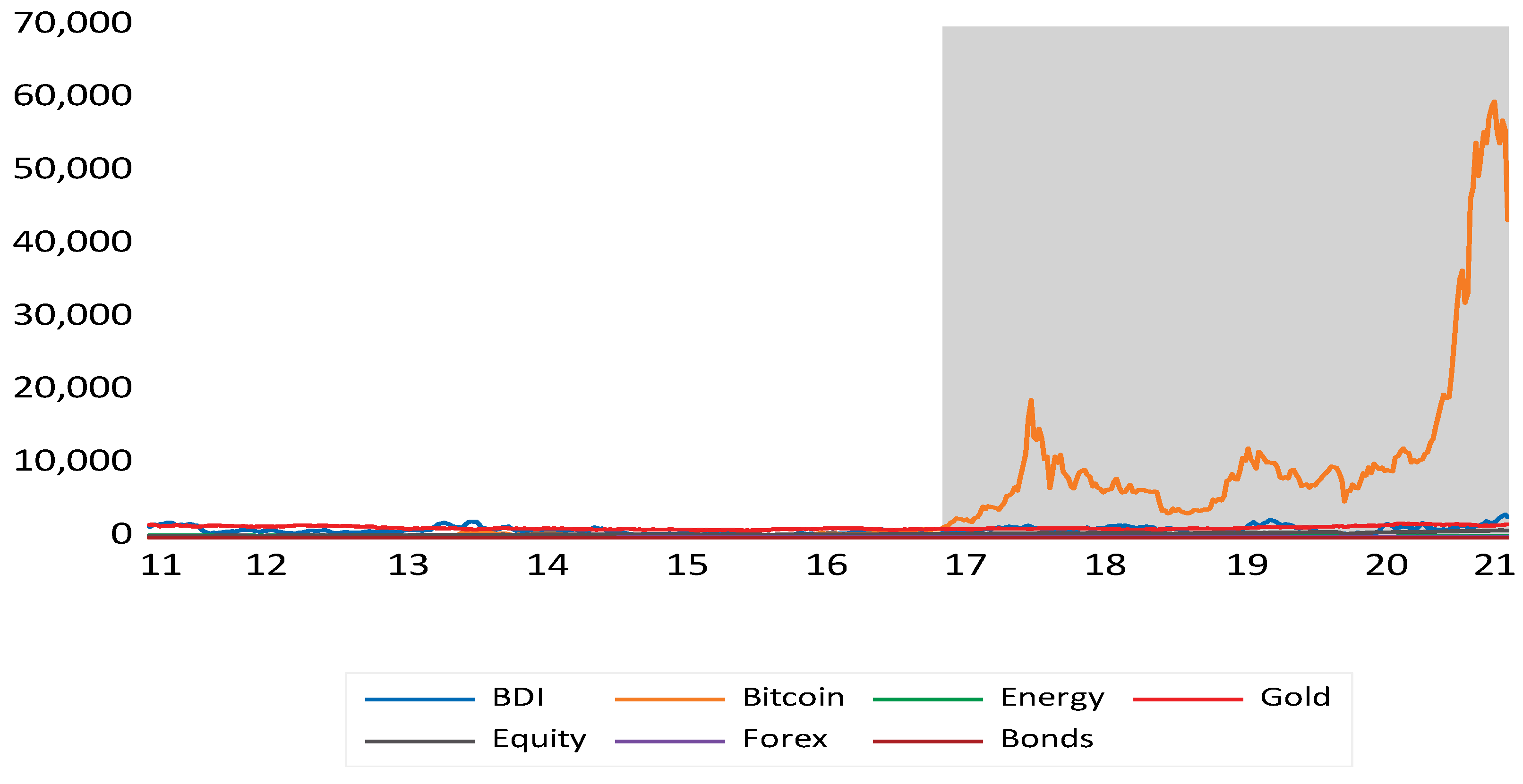
The descriptive statistics for all variables are presented in Table 2 below. The average return on Bitcoin was considerably higher than other assets during the sample period. The return on Bitcoin corresponded to 84% on an annualized basis, which was much higher than any other asset during the same period. However, the minimum and maximum Bitcoin returns also showed that there were more extreme price movements in Bitcoin compared to other assets as well as a considerably higher standard deviation. The extreme and volatile nature of Bitcoin returns was also reflected by its high kurtosis value (11.50) along with a high standard deviation compared to other assets in the panel. One of the possible reasons for this behavior could be the drastic price spike of Bitcoin during 2017 and in early 2021 where prices increased exponentially, remaining considerably volatile in the intervening periods and thereafter. The price development of all assets and Bitcoin is presented in Figure 1 below, clearly highlighting the explosive price development of Bitcoin compared to other assets.
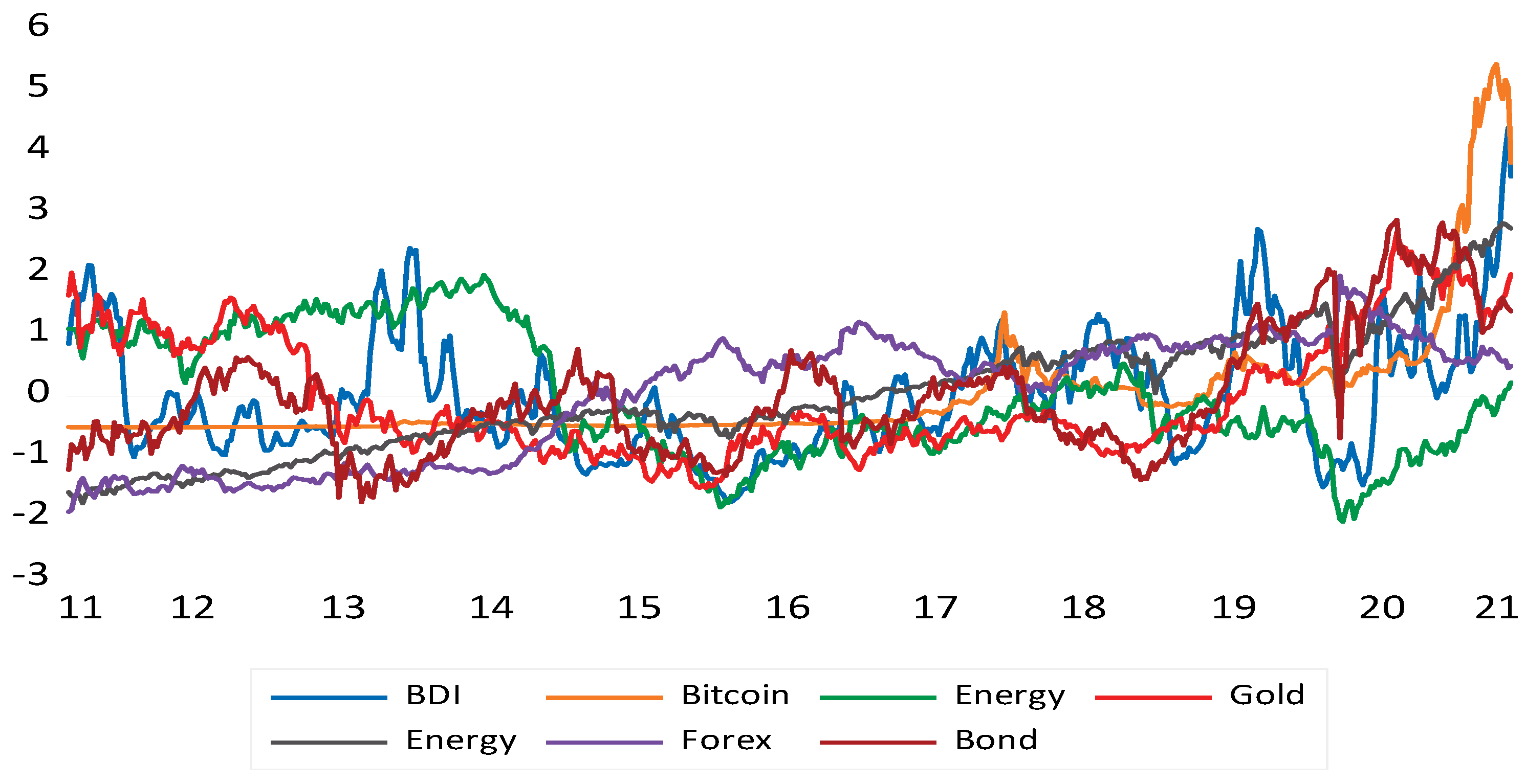
Moreover, the graph of normalized price development (Figure 2) shows that Bitcoin price volatility initially increased after the price spike of 2017 and then again in early 2021 in the post-COVID, speculative and uncertain regulatory environment regarding the mainstreaming of Bitcoin, environmental concerns, and regulatory crackdowns. In addition, the graph indicates that Bitcoin exhibited the largest variance in its prices during the sample period, particularly after 2017. Bitcoin prices remained considerably stable from the period 2011–2017; however, due to the increased popularity of Bitcoin subsequently, the prices saw some unusual price movements with a varying degree of correlation to different asset classes. As shown in Figure 2 above, Bitcoin exhibited a tendency to be negatively correlated with some asset classes during market downturns such as the one witnessed during the COVID-19 crisis while moving in tandem to varying degrees with major asset classes under study, on average. To further understand Bitcoin’s potential to act as a portfolio diversifier, a hedge, or a safe haven, further analysis was performed to demonstrate the limits of Bitcoin as an investment alternative. The correlation results are presented below in Table 3. Given the definition of a hedge, diversifier, and safe haven given by Baur and Lucey (2010), Bitcoin could at most act as a diversifier due to its low to medium correlation with other assets, as indicated in the correlation results in Table 3 below. Baur and Lucey (2010) defined a diversifier as an asset that was, on average, positively, but not perfectly, correlated with other assets. As indicated by the correlation matrix in Table 3, Bitcoin appeared to have low to medium potential for acting as a diversifier, owing to its low correlation with other assets (mostly ). Moreover, the highest positive correlation for Bitcoin was reported with gold (, and thus, the asset Bitcoin resembled in terms of price movements and price development was gold, but the correlation coefficient might be too small to classify it in the same category of assets as gold.
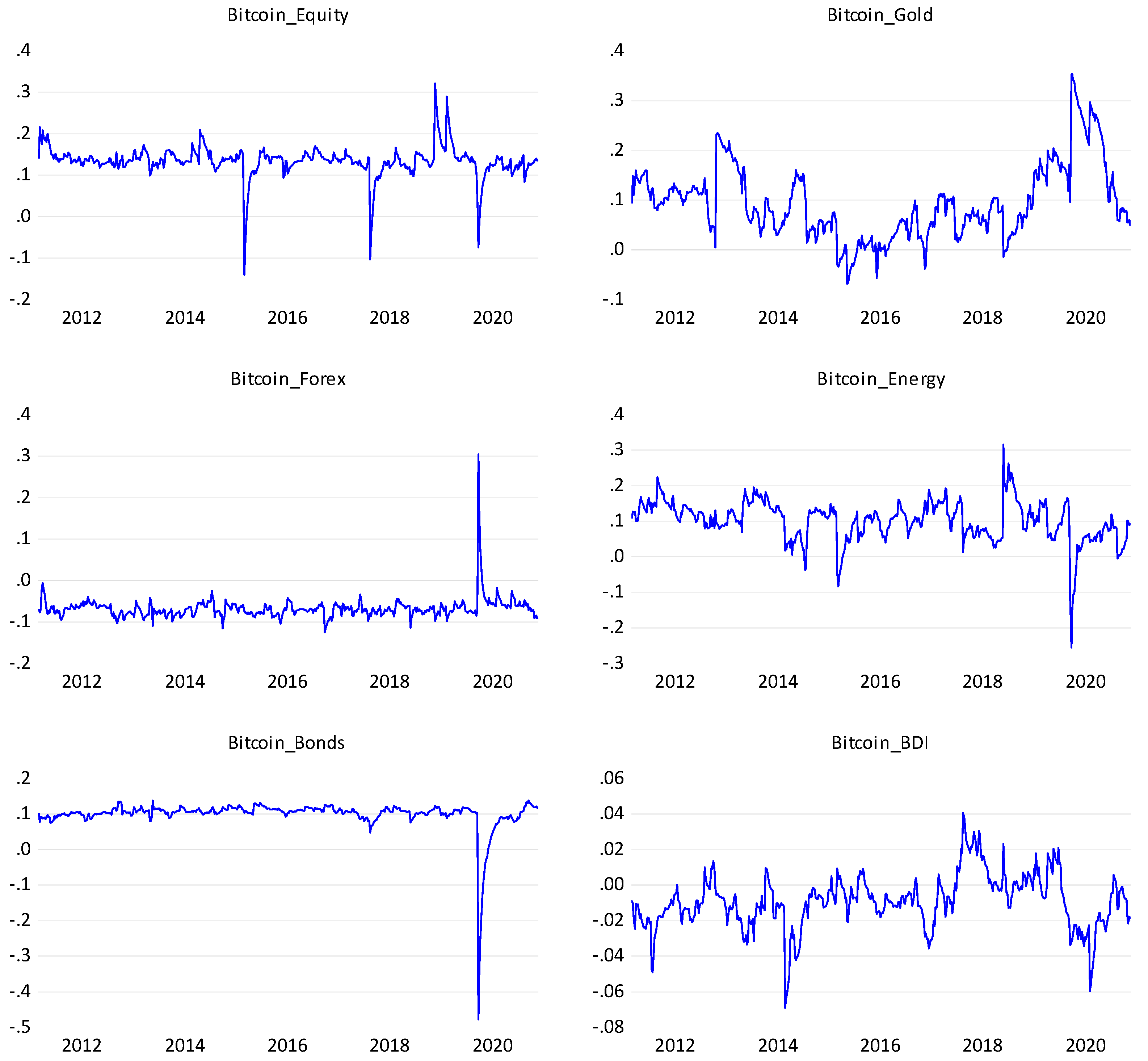
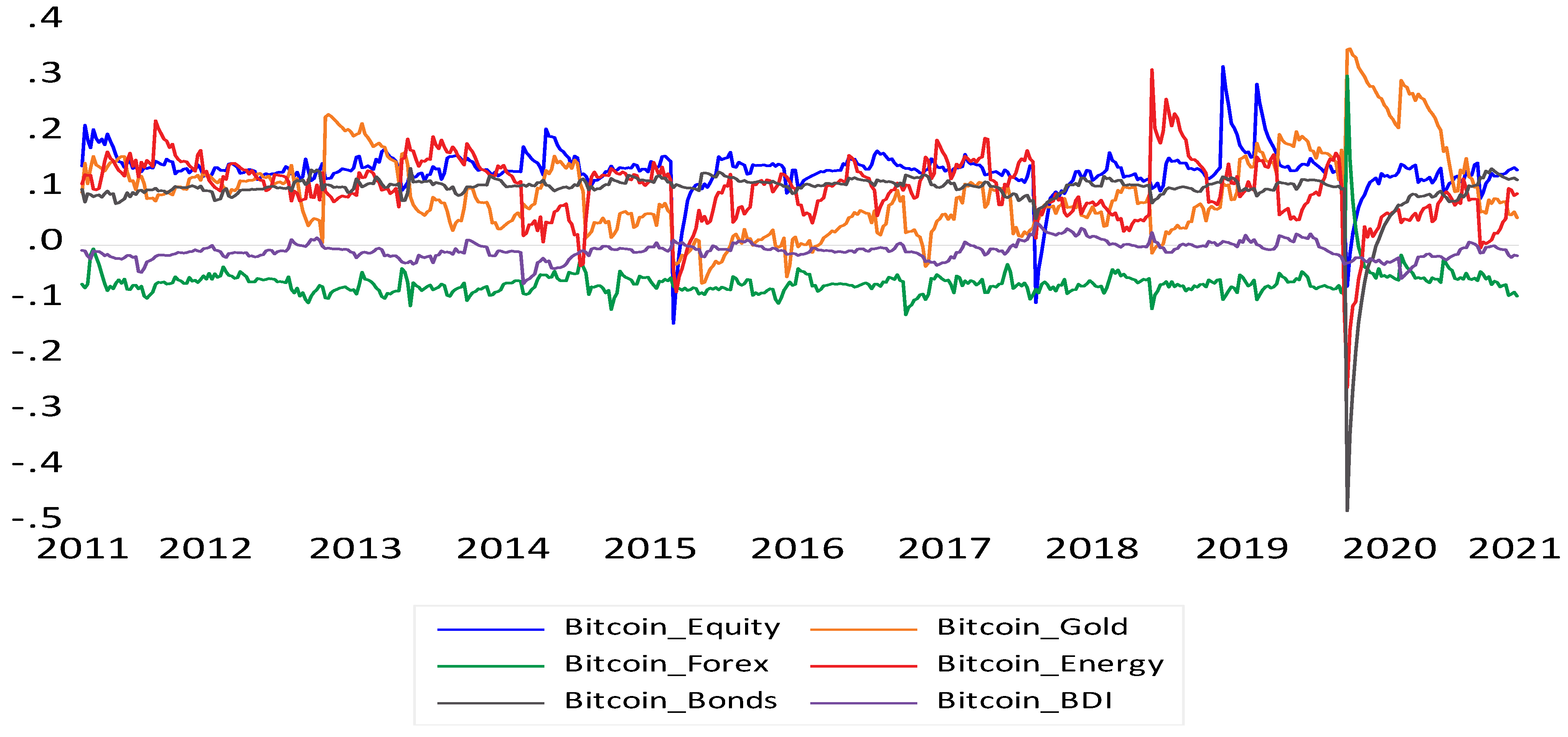
Because the point estimate of correlation might not always present a reasonable depiction of the nature of correlation, further analysis was carried out to study the dynamic conditional correlation between Bitcoin and other assets, an approach followed by Ngene et al. (2018) to investigate the presence of time–invariant interactions in volatility between assets (or markets). The results of the dynamic conditional correlation are presented in Figure 3 below. The graph depicts that Bitcoin exhibited a very low level of dynamic conditional correlation with most of the asset classes while exhibiting a negative correlation with Forex and BDI, on average. It must also be pointed out that Bitcoin exhibited a strong positive correlation with gold during extreme market conditions, particularly during the COVID-19 crisis, thereby demonstrating some resemblance of Bitcoin to gold. In addition, during early 2020, there was a sharp dip in the correlations between Bitcoin and other assets, which may indicate some potential for Bitcoin to be classified between a hedge and safe haven, according to the generally agreed definitions of Baur and Lucey (2010). More graphical evidence suggesting the potential of Bitcoin as a diversifier, hedge, or safe haven is presented in Appendix A.
Based on the preliminary evaluation above, the present study, therefore, evaluated the diversification potential of Bitcoin, using the portfolio optimization approach discussed in Section 4.2 below.
4.2. Portfolio Optimization and Monte Carlo Simulation
The analysis comprised a total of 8 optimization scenarios based on different constraining (or unconstrained) frameworks. The scenarios included naïve (or equal-weighted) portfolios, risk-parity portfolios, unconstrained portfolios, and semi-constrained portfolios. A detailed discussion on the construction of these frameworks is provided in the methodology section. It must be pointed out here that some scenarios were dropped from the analysis due to irrational outcomes. For the remaining portfolio frameworks, the portfolios were compared in terms of portfolio mean weekly return, mean weekly risk–return ratio (Sharpe ratio), historical VaR (HS VaR), variance–covariance VaR (VCV VaR), and conditional VaR (HS CVaR, VCV CVaR) for portfolios with and without Bitcoin. The portfolio results were then simulated with 10,000 iterations, using the Monte Carlo simulation approach. The portfolios were then compared based on their Monte Carlo simulation outcomes—mean-variance risk-adjusted returns, the Sharpe ratio, and Monte Carlo simulation-based CVaR (MC CVaR). The key results are presented in Table 4, Table 5, Table 6 and Table 7 below.
The results shown in Table 4 and Table 6 indicate that for almost all portfolio frameworks except risk parity portfolios (Scenarios 5 and 6), the mean returns, standard deviation, risk-adjusted returns, and VaR for a portfolio with Bitcoin were higher than that of a portfolio without Bitcoin. For the naïve portfolio (Scenario 1), the optimized mean-variance portfolio with a Bitcoin weight of 14.29% compared to a no-Bitcoin portfolio showed a considerable improvement in the risk-adjusted return performance. The mean returns showed a considerable increase from 0.071% to 0.292% with a modest increase in standard deviation from 1.97% to 2.58% and subsequently, a considerable increase in the Sharpe ratio from 3.58 to 11.28% when including Bitcoin in the portfolio. Likewise, in a semi-constrained max-long portfolio (Scenario 2), the optimized portfolio suggested a Bitcoin weight of 2.95%. It must be noted that under this scenario, the mean returns increased from 0.087% to 0.255%, and the standard deviation mildly increased from 0.90% to 1.64% with a considerable jump in the Sharpe ratio from 9.68% to 15.57% after adding Bitcoin into the portfolio optimization (within given constraints). Similar results were presented in scenario 3, a semi-constrained min-long portfolio with a Bitcoin weight of 10%; under this framework, when including Bitcoin in the portfolio, the mean returns increased from 0.146% to 0.386%, while the portfolio’s standard deviation only increased from 1.76% to 2.81%, consequently leading to a significant tick in the Sharpe ratio from 8.28% to 13.74%. It must also be noted that Scenario 2 and Scenario 4 presented similar results, thereby suggesting that there was no impact of shorting on the portfolio optimization if the long position was constrained in each asset. Surprisingly, under naïve and semi-constrained portfolio frameworks, VaR did not sharply increase with the inclusion of Bitcoin in the portfolio. It must, however, be noted that the portfolios with Bitcoin had a tendency to suffer considerable losses under extreme market conditions, as can be seen from portfolio CVaR. Moreover, the variance–covariance approach appeared to underestimate losses during extreme market conditions compared to historical estimates of CVaR while almost reporting VaR consistent with the historical performance of the portfolio under normal market conditions.
Similar results were reported under Scenarios 5 to Scenario 8 in regard to mean-variance performance of the portfolio. Risk parity portfolios indicated that the standard deviation of portfolios with Bitcoin was somewhat less than the portfolios without Bitcoin, which could be understood due to the fact that each asset contributed equally to the overall portfolio risk. Therefore, the weights of assets with a higher risk contribution to the portfolio were significantly reduced. These results were consistent with Ngene et al. (2018), who reported that the risk parity weights of risky assets should be lower, and the risk parity weights of less risky assets should be higher in a risk-parity portfolio. Scenario 5—Risk Parity (Long Only) Portfolio was optimized under the no shorting constraint; under this scenario, the average returns increased from 0.064% to 0.123% by allocating 4.90% of the portfolio to Bitcoin. The Sharpe ratio also witnessed a moderate increase, and as one would expect, the VaR and CVaR estimates were almost in a similar range for both portfolios, strongly in support of the evidence that risk parity portfolios are somewhat tolerant to extreme market conditions in a particular asset class. In portfolio optimization Scenario 6—Risk Parity (Unconstrained) Portfolio; the Bitcoin was allocated 8.84% of total portfolio weight, resulting in an increase in the mean returns from 0.084% to 0.155% through such allocations to Bitcoin. This framework with no constraint on shorting, however, also witnessed a sharp decrease in the CVaR in the portfolio with Bitcoin compared to the portfolio without Bitcoin. Scenario 7 represented a traditional framework that sought to maximize the Sharpe ratio with a no-shorting constraint, while Scenario 8 sought to maximize the Sharpe ratio with no constraint on shorting. Under both these scenarios, it could be observed that a considerably small allocation was made to Bitcoin (0.29% in Scenario 7 and 0.44% in Scenario 8). Regardless of the size of the allocation, the portfolio performance saw considerable improvement; the average returns under Scenario 7 increased from 0.087% to 0.125%, while the standard deviation witnessed a mild increase from 0.48% to 0.68%. The Sharpe ratio also witnessed a mild increase from 18.35% to 20.83%. Likewise, in Scenario 8, the average returns increased from 0.093% to 0.137%, the standard deviation increased from 0.51% to 0.65%, and the Sharpe ratio increased from 18.35% to 21.14%. It is important to point out here that the portfolio scenarios with limited exposure to Bitcoin (for instance, Scenario 7 and Scenario 8, risk parity portfolio excluded) did not witness extreme losses under extreme market conditions. It may, therefore, be prudent to conclude that while Bitcoin may offer considerable potential for portfolio diversification during normal market conditions, such allocations towards Bitcoin must be viewed with caution during extreme market conditions. Moreover, it can also be argued that Bitcoin may offer the potential for diversification to a risk-seeking investor, while it may not offer huge potential to a risk-averse investor. These results are consistent with the findings reported by Jeribi and Fakhfekh (2021), Pho et al. (2021), Garcia-Jorcano and Benito (2020), and Platanakis and Urquhart (2020) on the potential of Bitcoin as a diversifier. With the inclusion of Bitcoin in the portfolio, in addition to risk-adjusted return metrics, it also increased the variance, VaR, and CVaR of the portfolio; it can thus be concluded that Bitcoin clearly offered an upside in the return but simultaneously increased the risk of a well-diversified portfolio. Our findings revealed that adding Bitcoin to a well-diversified portfolio increased the risk-adjusted return considerably, particularly in constrained scenarios, as depicted by Scenarios 2 and 3, while there seemed to be only a moderate increase in the risk-adjusted performance of unconstrained portfolios (Scenarios 7 and 8). Moreover, Bitcoin appeared to be a potential diversifier for risk parity portfolios under both the constrained (long-only) and unconstrained frameworks, as witnessed by the increments in the risk-adjusted performance of these portfolios.
Contrary to the findings of Aggarwal et al. (2018) and DeMiguel et al. (2009), the results indicated that the risk-adjusted return performance of constrained portfolios was higher than naïve portfolios. One of the possible reasons for such performance under a strictly constrained portfolio could be that such portfolios tend to be similar to manually constructed portfolios, with a little flexibility for the maneuverability in weights to take the benefits of negative co-movements of the assets to generate better portfolio outcomes. Moreover, the results also showed that among the constraining scenarios, the best performance was observed for a semi-constrained max-long portfolio limiting the maximum position in any asset to 25 percent of the portfolio value with no shorting constraint. Our findings revealed that a semi-constrained max-long portfolio provided decent incremental mean-variance performance, captured by its Sharpe ratio, and that adding Bitcoin to this semi-constrained scenario caused a 5.89% increase in the Sharpe ratio with a considerably low HS CVaR (at 99% confidence interval). One way to explain these results is that because the Bitcoin market is populated by frenzy investors and witnesses huge and sometimes wild movements (Bouri et al. 2019; Tan and Low 2017), a carefully constraint-operated portfolio is deemed necessary for building a well-balanced portfolio while mitigating tolerable risk. In contrast, the increments in the Sharpe ratio for the naïve portfolio with Bitcoin and for the semi-constrained min-long portfolio (Scenario 3) were larger but with considerably higher extreme value CVaR estimates. The results also revealed that increasing the weight of Bitcoin generated incremental returns, but the risk increased disproportionately, resulting in a decrease in the Sharpe ratio, as observed in the Scenario 3 framework. It may, therefore, be concluded that including Bitcoin does not essentially increase the risk-adjusted performance of a portfolio unless carefully constrained. It may thus be reasonable to conclude that Bitcoin has considerable potential to increase the risk-adjusted returns of a well-diversified portfolio, and therefore, this establishes Bitcoin as an alternative investment that investors may consider while designing their investment policy strategies, specifically their asset allocation.
The simulation results shown in Table 5 and Table 7 also indicate that adding Bitcoin considerably increased the risk-adjusted return of portfolios with Bitcoin compared to the portfolios without Bitcoin under all frameworks. The simulation results were similar to variance–covariance-based metrics for obvious reasons and had a tendency to underestimate losses during extreme market conditions. It may, therefore, be concluded that besides the risk-adjusted return, the risk (or conditional value at risk) of a portfolio considerably increases by adding Bitcoin to a well-diversified portfolio, and thus, adding Bitcoin may be considered a bit too risky by risk-averse investors and thus has implications for the performance and actions of investment professionals.
5. Conclusions
Bitcoin has proven to be a fascinating and controversial addition to the global financial landscape; it is a cryptocurrency that has been simultaneously feted as a future alternative to official fiat currencies and disparaged as a disruptive and volatile play-thing of amateur speculators.
The results suggest that Bitcoin has some potential to act as a diversifier because in almost all the portfolio optimization frameworks, the performance attributes of the portfolios with Bitcoin were considerably higher compared to portfolios without Bitcoin. It must also be pointed out that the allocation to Bitcoin in most of the unconstrained or semi-constrained frameworks was minimal. It may, therefore, be concluded that because Bitcoin witnesses heavy price fluctuations, investors must exercise caution and limit their exposure to Bitcoin, as excess exposure to Bitcoin may not essentially lead to improvement in portfolio performance attributes. Moreover, the results also indicate that adding Bitcoin to a portfolio increases the conditional value at risk during extreme market conditions.
Against this backdrop, certainly, empirical evidence suggests that Bitcoin has been (until now) immune to economic and financial downturns, stock market downturns (Dyhrberg 2016b), and ill-conceived and ill-implemented monetary policy developments such as those of the Venezuelan government and the Indian demonetization experiment (Luther and Salter 2017; Bouoiyour and Selmi 2017; Selmi et al. 2018). However, although our results support the hypothesis that Bitcoin can play a significant role in portfolio diversification and investment management, it would be going too far to assert that Bitcoin can serve as an alternative asset due to its random spikes and movement in prices. Bitcoin’s price volatility is likely to be due to the lack of interest from the institutional investors who still consider Bitcoin a speculative asset and its price formation as a bubble fueled by young, inexperienced individual investors as well as being due to various legal, taxation, or accounting problems associated with cryptocurrency (Bouri et al. 2019; Tan and Low 2017). As such, considerably more evidence in Bitcoin’s favor is required before we can expect Bitcoin to be considered an alternative asset to commodities or gold.
That said, it will certainly be interesting to see how Bitcoin price development evolves as the legal, regulatory, and accounting guidelines with regard to it change. In addition, with the recent introduction of Bitcoin futures, the emergence of a strong altcoin market, and other developments (among them, uncertainty around the acceptance of Bitcoin on various platforms, such as, Elon Musk’s investment and commitment to accepting Bitcoin as a mode of payment and subsequent backtracking for environmental concerns, the crackdown on Bitcoin mining in China, etc.), it will be interesting to see whether significant economic, fiscal, and financial downturns such as those witnessed in recent periods will still render Bitcoin as a diversifier, hedge, or safe haven.
Author Contributions
Conceptualization, W.B., A.R., S.A.-M., and N.E.-K.; methodology, A.R.; software, A.R.; formal analysis, W.B., A.R., S.A.-M., and N.E.-K.; resources, W.B., A.R., S.A.-M., and N.E.-K.; data curation, W.B., A.R., S.A.-M., and N.E.-K.; writing—original draft preparation, W.B., A.R., S.A.-M., and N.E.-K.; writing—review and editing, W.B., A.R., S.A.-M., and N.E.-K. All authors have read and agreed to the published version of the manuscript.
Funding
This research received no external funding.
Institutional Review Board Statement
Not applicable.
Informed Consent Statement
Not applicable.
Conflicts of Interest
The authors declare no conflict of interest.
Appendix A. Supplemental Dynamic Conditional Correlation Graphs
Figure A1.
Dynamic conditional correlation—Bitcoin with all assets (DCC-GARCH). Note: The graph in Figure A1 suggests that Bitcoin exhibits a negative conditional correlation with Forex and BDI, while it exhibits a very low correlation with other assets throughout the sample period. The conditional correlation appears to sharply fluctuate (dip) during the periods of financial crisis (for instance, the COVID-19 crisis in early 2020), thereby suggesting some potential of Bitcoin as a hedge or safe haven against those assets.

Figure A2.
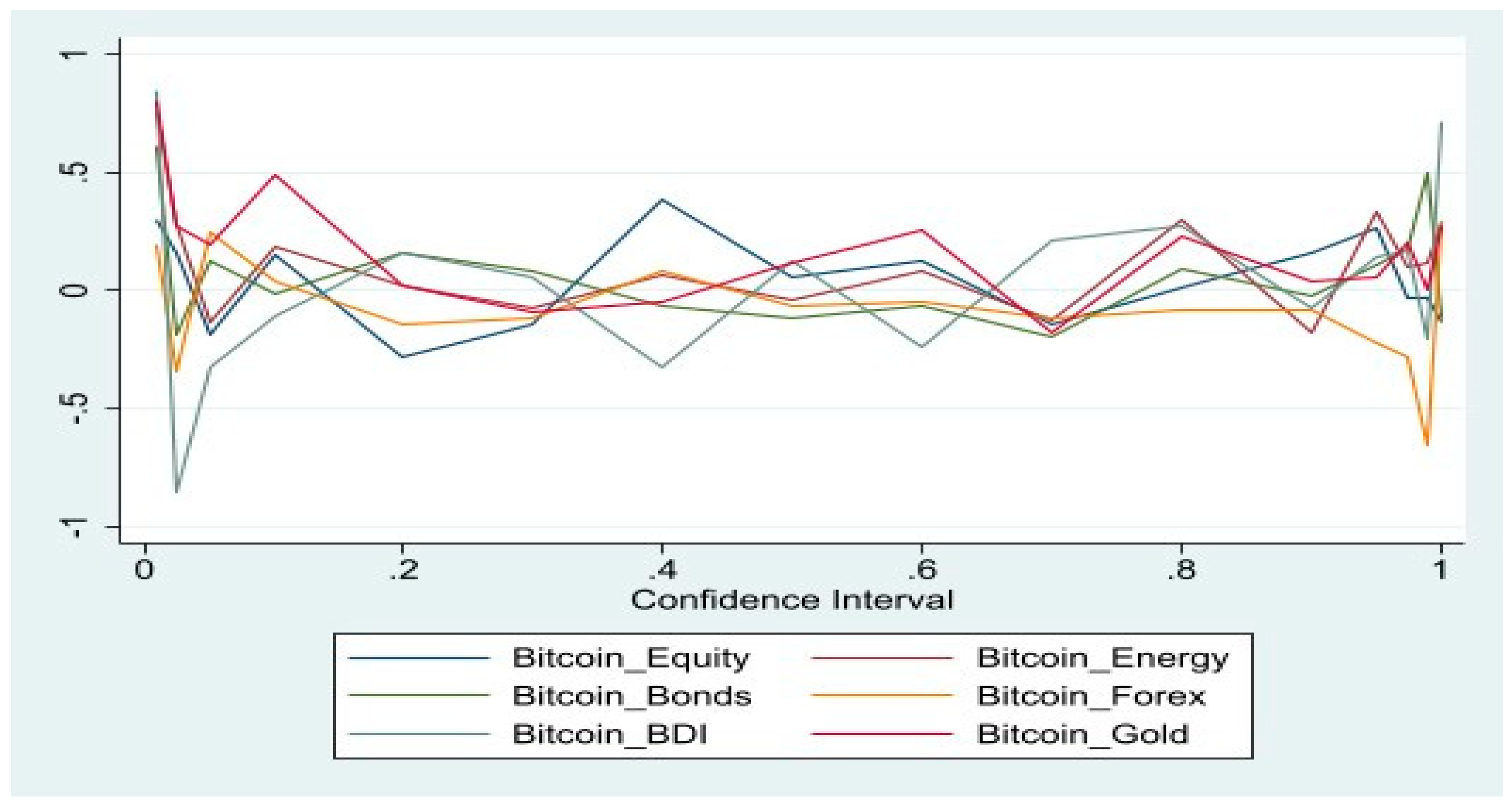
Dynamic conditional correlation—Bitcoin with all assets (DCC-GARCH). Note: The graph in Figure A2 suggests that Bitcoin exhibits negative dynamic conditional correlation at low confidence intervals (negative price development of the reference asset) with a considerably low to negative correlation with all assets during normal price evolution. This indicates that Bitcoin may serve as a potential diversifier, while it may also have some potential properties ranging between a hedge and a safe haven; however, this property appears to dissipate with a slight change in the market conditions.
Figure A2.
Dynamic conditional correlation—Bitcoin with all assets (DCC-GARCH). Note: The graph in Figure A2 suggests that Bitcoin exhibits negative dynamic conditional correlation at low confidence intervals (negative price development of the reference asset) with a considerably low to negative correlation with all assets during normal price evolution. This indicates that Bitcoin may serve as a potential diversifier, while it may also have some potential properties ranging between a hedge and a safe haven; however, this property appears to dissipate with a slight change in the market conditions.

Appendix B
The table presents the detailed portfolio optimization results, indicating the weights of each asset under each constraining (or otherwise) framework, for portfolios with and without Bitcoin.

Table A1.
Portfolio Optimization Results.
| Constraining Framework | Scenario 1 Naïve Portfolio | Scenario 2 Semi-Constrained Max-Long Portfolio | Scenario 3 Semi-Constrained Min-Long Portfolio | Scenario 4 Constrained Portfolio | ||||
| Without Bitcoin | With Bitcoin | Without Bitcoin | With Bitcoin | Without Bitcoin | With Bitcoin | Without Bitcoin | With Bitcoin | |
| Asset/Index | ||||||||
| Forex | 16.67% | 14.29% | 25.00% | 25.00% | 10.00% | 10.00% | 25.00% | 25.00% |
| Bitcoin | - | 14.29% | - | 2.95% | - | 10.00% | - | 2.95% |
| Baltic Dry Index | 16.67% | 14.29% | 2.65% | 10.31% | 10.00% | 17.66% | 2.65% | 10.31% |
| Equities | 16.67% | 14.29% | 25.00% | 25.00% | 50.00% | 32.34% | 25.00% | 25.00% |
| Energy | 16.67% | 14.29% | 0.36% | −1.99% | 10.00% | 10.00% | 0.36% | −1.99% |
| Corporate Bond | 16.67% | 14.29% | 25.00% | 25.00% | 10.00% | 10.00% | 25.00% | 25.00% |
| Gold | 16.67% | 14.29% | 21.98% | 13.74% | 10.00% | 10.00% | 21.98% | 13.74% |
| Average Returns ( | 0.071% | 0.292% | 0.087% | 0.255% | 0.146% | 0.386% | 0.087% | 0.255% |
| Standard Deviation | 1.97% | 2.58% | 0.90% | 1.64% | 1.76% | 2.81% | 0.90% | 1.64% |
| Sharpe Ratio | 3.58% | 11.29% | 9.68% | 15.57% | 8.28% | 13.74% | 9.68% | 15.57% |
| Constraining Framework | Scenario 5 Risk Parity (Long Only) Portfolio | Scenario 6 Risk Parity (Unconstrained) Portfolio | Scenario 7 Long Only Portfolio | Scenario 8 Unconstrained Portfolio | ||||
| Without Bitcoin | With Bitcoin | Without Bitcoin | With Bitcoin | Without Bitcoin | Without Bitcoin | With Bitcoin | Without Bitcoin | |
| Asset/Index | ||||||||
| Forex | 0.00% | 6.04% | −118.94% | −28.69% | 66.64% | 66.60% | 67.08% | 67.18% |
| Bitcoin | - | 4.90% | - | 8.84% | - | 0.29% | - | 0.44% |
| Baltic Dry Index | 5.84% | 3.14% | 14.60% | 5.53% | 0.28% | 2.40% | 0.39% | 2.61% |
| Equities | 19.76% | 22.75% | 43.20% | 23.08% | 20.59% | 20.25% | 22.62% | 22.96% |
| Energy | 13.00% | 9.95% | 28.62% | 15.21% | 0.00% | 0.00% | −2.34% | −3.16% |
| Corporate Bond | 37.00% | 27.22% | 79.94% | 48.96% | 5.05% | 5.60% | 4.56% | 4.99% |
| Gold | 24.41% | 25.99% | 52.59% | 27.07% | 7.44% | 4.86% | 7.68% | 4.98% |
| Average Returns ( | 0.064% | 0.123% | 0.084% | 0.155% | 0.087% | 0.125% | 0.093% | 0.137% |
| Standard Deviation | 1.37% | 1.36% | 3.61% | 2.06% | 0.48% | 0.60% | 0.51% | 0.65% |
| Sharpe Ratio | 4.67% | 9.03% | 2.34% | 7.49% | 18.11% | 20.83% | 18.35% | 21.14% |
| 1 | Data is available online: https://www.coindesk.com/price/Bitcoin (accessed on 10 June 2021). |
| 2 | Data is available online: https://www.coindesk.com/price/Bitcoin (accessed on 10 June 2021). |
| 3 | Data is available online: https://www.bloomberg.com/quote/BDIY:IND (accessed on 10 May 2020). |
| 4 | Data is available online: https://www.coindesk.com/price/Bitcoin (accessed on 10 June 2021). |
References
- Aggarwal, Shivani, Mayank Santosh, and Prateek Bedi. 2018. Bitcoin and Portfolio Diversification: Evidence from India. In Digital India. Cham: Springer, pp. 99–115. [Google Scholar]
- Andrianto, Yanuar, and Diputra Yoda. 2017. The effect of cryptocurrency on investment portfolio effectiveness. Journal of Finance and Accounting 5: 229–38. [Google Scholar] [CrossRef] [Green Version]
- Baek, Chung, and Matt Elbeck. 2015. Bitcoins as an investment or speculative vehicle? A first look. Applied Economics Letters 22: 30–4. [Google Scholar] [CrossRef]
- Baumöhl, Eduard. 2019. Are cryptocurrencies connected to forex? A quantile cross-spectral approach. Finance Research Letters 29: 363–72. [Google Scholar] [CrossRef]
- Baur, Dirk, and Brian Lucey. 2010. Is gold a hedge or a safe haven? An analysis of stocks, bonds and gold. Financial Review 45: 217–29. [Google Scholar] [CrossRef]
- Baur, Dirk, Kihoon Hong, and Adrian Lee. 2018. Bitcoin: Medium of exchange or speculative assets? Journal of International Financial Markets, Institutions and Money 54: 177–89. [Google Scholar] [CrossRef]
- Beckmann, Joscha, Theo Berger, and Robert Czudaj. 2015. Does gold act as a hedge or a safe haven for stocks? A smooth transition approach. Economic Modelling 48: 16–24. [Google Scholar] [CrossRef] [Green Version]
- Blau, Benjamin. 2017. Price dynamics and speculative trading in Bitcoin. Research in International Business and Finance 41: 493–99. [Google Scholar] [CrossRef]
- Boiko, Viktor, Yelizaveta Tymoshenko, Anna Kononenko, and Dmitrii Goncharov. 2021. The optimization of the cryptocurrency portfolio in view of the risks. Journal of Management Information and Decision Sciences 24: 1–9. [Google Scholar]
- Bouoiyour, Jamal, and Refk Selmi. 2017. The Bitcoin price formation: Beyond the fundamental sources. arXiv arXiv:1707.01284. [Google Scholar]
- Bouoiyour, Jamal, Refk Selmi, Aviral Tiwari, and Olaolu Olayeni. 2016. What drives Bitcoin price. Economics Bulletin 36: 843–50. [Google Scholar]
- Bouri, Elie, Naji Jalkh, Peter Molnár, and David Roubaud. 2017a. Bitcoin for energy commodities before and after the December 2013 crash: Diversifier, hedge or safe haven? Applied Economics 49: 5063–73. [Google Scholar] [CrossRef]
- Bouri, Elie, Peter Molnár, Georges Azzi, David Roubaud, and Lars Hagfors. 2017b. On the hedge and safe haven properties of Bitcoin: Is it really more than a diversifier? Finance Research Letters 20: 192–98. [Google Scholar] [CrossRef]
- Bouri, Elie, Rangan Gupta, Aviral Tiwari, and David Roubaud. 2017c. Does Bitcoin hedge global uncertainty? Evidence from wavelet-based quantile-in-quantile regressions. Finance Research Letters 23: 87–95. [Google Scholar] [CrossRef] [Green Version]
- Bouri, Elie, Rangan Gupta, Chi Lau, David Roubaud, and Shixuan Wang. 2018. Bitcoin and global financial stress: A copula-based approach to dependence and causality in the quantiles. The Quarterly Review of Economics and Finance 69: 297–307. [Google Scholar] [CrossRef] [Green Version]
- Bouri, Elie, Rangan Gupta, and David Roubaud. 2019. Herding behaviour in cryptocurrencies. Finance Research Letters 29: 216–21. [Google Scholar] [CrossRef]
- Bouri, Elie, Syed Shahzad, David Roubaud, Ladislav Kristoufek, and Brian Lucey. 2020. Bitcoin, gold, and commodities as safe havens for stocks: New insight through wavelet analysis. The Quarterly Review of Economics and Finance 77: 156–64. [Google Scholar] [CrossRef]
- Brauneis, Alexander, and Roland Mestel. 2018. Price discovery of cryptocurrencies: Bitcoin and beyond. Economics Letters 165: 58–61. [Google Scholar] [CrossRef]
- Brian, Domitrovic. 2008. The Dollar—Euro Exchange Rate Sure Is the Most Imporant Price in the World. Forbes. Available online: https://www.forbes.com/sites/briandomitrovic/2018/02/06/the-dollar-euro-exchange-rate-sure-is-the-most-important-price-in-the-world/?sh=171921a2412b (accessed on 10 May 2020).
- Brière, Marie, Kim Oosterlinck, and Ariane Szafarz. 2015. Virtual Currency, Tangible Return: Portfolio Diversification with Bitcoin. Journal of Asset Management 16: 365–73. [Google Scholar] [CrossRef]
- Burnie, Andrew. 2018. Exploring the interconnectedness of cryptocurrencies using correlation networks. arXiv arXiv:1806.06632. [Google Scholar]
- Cai, Xiaoqiang, Kok-Lay Teo, Xiaoqi Yang, and Xun Yu Zhou. 2000. Portfolio optimization under a minimax rule. Management Science 46: 957–72. [Google Scholar] [CrossRef]
- Carrick, Jon. 2016. Bitcoin as a complement to emerging market currencies. Emerging Markets Finance and Trade 52: 2321–34. [Google Scholar] [CrossRef]
- Chan, Wing Hong, Minh Le, and Yan Wendy Wu. 2019. Holding Bitcoin longer: The dynamic hedging abilities of Bitcoin. The Quarterly Review of Economics and Finance 71: 107–13. [Google Scholar] [CrossRef]
- Cheah, Eng-Tuck, and John Fry. 2015. Speculative bubbles in Bitcoin markets? An empirical investigation into the fundamental value of the Bitcoin. Economics Letters 130: 32–36. [Google Scholar] [CrossRef] [Green Version]
- Chung, Pin J., and Donald. J. Liu. 1994. Common stochastic trends in Pacific Rim stock markets. The Quarterly Review of Economics and Finance 34: 241–59. [Google Scholar] [CrossRef]
- Ciaian, Pavel, Miroslava Rajcaniova, and d’Artis Kancs. 2016. The economics of Bitcoin price formation. Applied Economics 48: 1799–815. [Google Scholar] [CrossRef] [Green Version]
- Ciner, Cetin. 2001. On the long run relationship between gold and silver prices A note. Global Finance Journal 12: 299–303. [Google Scholar] [CrossRef]
- Ciner, Cetin, Constantin Gurdgiev, and Brian Lucey. 2013. Hedges and safe havens: An examination of stocks, bonds, gold, oil and exchange rates. International Review of Financial Analysis 29: 202–11. [Google Scholar] [CrossRef]
- Click, Reid, and Michael Plummer. 2005. Stock market integration in ASEAN after the Asian financial crisis. Journal of Asian Economics 16: 5–28. [Google Scholar] [CrossRef]
- Colombo, Jefferson, Fernando Cruz, Luis Paese, and Renan Cortes. 2021. The Diversification Benefits of Cryptocurrencies in Multi-Asset Portfolios: Cross-Country Evidence. Available online: https://papers.ssrn.com/sol3/papers.cfm?abstract_id=3776260 (accessed on 12 June 2021).
- Conrad, Christian, Anessa Custovic, and Eric Ghysels. 2018. Long-and short-term cryptocurrency volatility components: A GARCH-MIDAS analysis. Journal of Risk and Financial Management 11: 23. [Google Scholar] [CrossRef]
- DeFusco, Richard, John Geppert, and George Tsetsekos. 1996. Long-run diversification potential in emerging stock markets. Financial Review 31: 343–63. [Google Scholar] [CrossRef]
- DeMiguel, Victor, Lorenzo Garlappi, Francisco Nogales, and Raman Uppal. 2009. A generalized approach to portfolio optimization: Improving performance by constraining portfolio norms. Management Science 55: 798–812. [Google Scholar] [CrossRef] [Green Version]
- Deng, Guang-Feng, Woo-Tsong Lin, and Chih-Chung Lo. 2012. Markowitz-based portfolio selection with cardinality constraints using improved particle swarm optimization. Expert Systems with Applications 39: 4558–66. [Google Scholar] [CrossRef]
- Dwyer, Gerald P. 2015. The economics of Bitcoin and similar private digital currencies. Journal of Financial Stability 17: 81–91. [Google Scholar] [CrossRef] [Green Version]
- Dyhrberg, Anne Haubo. 2016a. Hedging capabilities of bitcoin. Is it the virtual gold? Finance Research Letters 16: 139–44. [Google Scholar] [CrossRef] [Green Version]
- Dyhrberg, Anne Haubo. 2016b. Bitcoin, gold and the dollar—A GARCH volatility analysis. Finance Research Letters 16: 85–92. [Google Scholar] [CrossRef] [Green Version]
- Dyhrberg, Anne Haubo, Sean Foley, and Jiri Svec. 2018. How investible is Bitcoin? Analyzing the liquidity and transaction costs of Bitcoin markets. Economics Letters 171: 140–43. [Google Scholar] [CrossRef]
- Ehrgott, Matthias, Kathrin Klamroth, and Christian Schwehm. 2004. An MCDM approach to portfolio optimization. European Journal of Operational Research 155: 752–70. [Google Scholar] [CrossRef]
- Eisl, Alexander, Stephan Gasser, and Stephan Weinmayer. 2015. Caveat Emptor: Does Bitcoin Improve Portfolio Diversification? Available online: https://papers.ssrn.com/sol3/papers.cfm?abstract_id=2408997 (accessed on 8 June 2021).
- Ferson, Wayne, Suresh Nallareddy, and Biqin Xie. 2013. The “out-of-sample” performance of long run risk models. Journal of Financial Economics 107: 537–56. [Google Scholar] [CrossRef]
- Gaivoronski, Alexei, and Georg Pflug. 2005. Value-at-risk in portfolio optimization: Properties and computational approach. The Journal of Risk 7: 1–31. [Google Scholar] [CrossRef] [Green Version]
- Gangwal, Shashwat. 2017. Analyzing the effects of adding Bitcoin to portfolio. International Journal of Economics and Management Engineering 10: 3519–32. [Google Scholar]
- Garcia, David, Claudio Tessone, Pavlin Mavrodiev, and Nicolas Perony. 2014. The digital trace of bubbles: Feedback cycles between socio-economic signals in the Bitcoin economy. Journal of the Royal Society Interface 11: 623–31. [Google Scholar] [CrossRef] [PubMed]
- Garcia-Jorcano, Laura, and Sonia Benito. 2020. Studying the properties of the Bitcoin as a diversifying and hedging asset through a copula analysis: Constant and time-varying. Research in International Business and Finance 54: 1–24. [Google Scholar] [CrossRef]
- Glaser, Florian, Kai Zimmermann, Martin Haferkorn, Moritz Christian Weber, and Michael Siering. 2014. Bitcoin-Asset or Currency? Revealing Users’ Hidden Intentions. Available online: https://papers.ssrn.com/sol3/papers.cfm?abstract_id=2425247 (accessed on 25 May 2020).
- Guesmi, Khaled, Samir Saadi, Ilyes Abid, and Zied Ftiti. 2019. Portfolio diversification with virtual currency: Evidence from bitcoin. International Review of Financial Analysis 63: 431–37. [Google Scholar] [CrossRef]
- Ivanova, Miroslava, and Lilko Dospatliev. 2017. Application of Markowitz portfolio optimization on Bulgarian stock market from 2013 to 2016. International Journal of Pure and Applied Mathematics 117: 291–307. [Google Scholar] [CrossRef] [Green Version]
- Jagannathan, Ravi, and Tongshu Ma. 2003. Risk reduction in large portfolios: Why imposing the wrong constraints helps. The Journal of Finance 58: 1651–83. [Google Scholar] [CrossRef] [Green Version]
- Jeribi, Ahmed, and Mohamed Fakhfekh. 2021. Portfolio management and dependence structure between cryptocurrencies and traditional assets: Evidence from FIEGARCH-EVT-Copula. Journal of Asset Management 22: 224–39. [Google Scholar] [CrossRef]
- Ji, Qiang, Elie Bouri, Rangan Gupta, and David Roubaud. 2018. Network causality structures among Bitcoin and other financial assets: A directed acyclic graph approach. The Quarterly Review of Economics and Finance 70: 203–13. [Google Scholar] [CrossRef] [Green Version]
- Kajtazi, Anton, and Andrea Moro. 2017. Bitcoin, portfolio diversification and Chinese financial Markets. Available online: https://papers.ssrn.com/sol3/papers.cfm?abstract_id=3062064 (accessed on 15 May 2020).
- Kajtazi, Anton, and Andrea Moro. 2019. The role of bitcoin in well diversified portfolios: A comparative global study. International Review of Financial Analysis 61: 143–57. [Google Scholar] [CrossRef] [Green Version]
- Kandel, Shmuel, and Robert Stambaugh. 1987. On correlations and inferences about mean-variance efficiency. Journal of Financial Economics 18: 61–90. [Google Scholar] [CrossRef]
- Karalevicius, Vytautas, Niels Degrande, and Jochen De Weerdt. 2018. Using sentiment analysis to predict interday Bitcoin price movements. The Journal of Risk Finance 19: 56–7. [Google Scholar] [CrossRef]
- Kaul, Aditya, and Sapp Stephen. 2006. Y2K fears and safe haven trading of the US dollar. Journal of International Money and Finance 25: 760–79. [Google Scholar] [CrossRef]
- Khaki, Audil, Somar Al-Mohamad, Walid Bakry, and Samet Gunay. 2020. Can Cryptocurrencies Be the Future Safe-Haven for Investors? A Case Study of Bitcoin. Working Paper. SSRN-ID 3593508. Available online: https://papers.ssrn.com/sol3/papers.cfm?abstract_id=3593508 (accessed on 30 October 2020).
- Koutmos, Dimitrios. 2018. Bitcoin returns and transaction activity. Economics Letters 167: 81–85. [Google Scholar] [CrossRef]
- Kristoufek, Ladislav. 2015. What are the main drivers of the Bitcoin price? Evidence from wavelet coherence analysis. PLoS ONE 10: e0123923. [Google Scholar] [CrossRef]
- Krokhmal, Pavlo, Palmquist Jonas, and Uryasev Stanislav. 2002. Portfolio optimization with conditional value-at-risk objective and constraints. Journal of Risk 4: 43–68. [Google Scholar] [CrossRef] [Green Version]
- Lee, Wai. 2011. Risk-based asset allocation: A new answer to an old question? The Journal of Portfolio Management 37: 11–28. [Google Scholar] [CrossRef]
- Luther, William, and Alexander Salter. 2017. Bitcoin and the bailout. The Quarterly Review of Economics and Finance 66: 50–56. [Google Scholar] [CrossRef]
- Ma, Yechi, Ferhana Ahmad, Miao Liu, and Zilong Wang. 2020. Portfolio optimization in the era of digital financialization using cryptocurrencies. Technological Forecasting and Social Change 161: 1–11. [Google Scholar] [CrossRef]
- Markowitz, Harry. 1952. Portfolio Selection. Journal of Finance 7: 77–91. [Google Scholar]
- Markowitz, Harry. 1958. Portfolio Selection: Efficient Diversification of Investments. New York: John Wiley & Sons. [Google Scholar]
- Mazanec, Jaroslav. 2021. Portfolio Optimalization on Digital Currency Market. Journal of Risk and Financial Management 14: 160. [Google Scholar] [CrossRef]
- Mendes, R. R. A., A. P. Paiva, Rogério Santana Peruchi, Pedro Paulo Balestrassi, Rafael Coradi Leme, and M. B. Silva. 2016. Multiobjective portfolio optimization of ARMA–GARCH time series based on experimental designs. Computers & Operations Research 66: 434–44. [Google Scholar]
- Miyazaki, Takashi, and Shigeyuki Hamori. 2014. Cointegration with regime shift between gold and financial variables. International Journal of Financial Research 5: 90–7. [Google Scholar] [CrossRef] [Green Version]
- Nadarajah, Saralees, and Jeffrey Chu. 2017. On the inefficiency of Bitcoin. Economics Letters 150: 6–9. [Google Scholar] [CrossRef] [Green Version]
- Nakamoto, Satoshi. 2008. Bitcoin: A Peer-to-Peer Electronic Cash System. Available online: https://nakamotoinstitute.org/bitcoin (accessed on 12 June 2021).
- Ngene, Geoffrey, Jordin Post, and Ann Mungai. 2018. Volatility and shock interactions and risk management implications: Evidence from the US and frontier markets. Emerging Markets Review 37: 181–98. [Google Scholar] [CrossRef]
- Nguyen, Sang Phu, and Toan Luu Duc Huynh. 2019. Portfolio optimization from a Copulas-GJRGARCH-EVT-CVAR model: Empirical evidence from ASEAN stock indexes. Quantitative Finance and Economics 3: 562–85. [Google Scholar] [CrossRef]
- Ozturk, Serda Selin. 2020. Dynamic Connectedness between Bitcoin, Gold, and Crude Oil Volatilities and Returns. Journal of Risk and Financial Management 13: 275. [Google Scholar] [CrossRef]
- Pal, Debdatta, and Subrata Mitra. 2019. Hedging bitcoin with other financial assets. Finance Research Letters 30: 30–36. [Google Scholar] [CrossRef]
- Pho, Kim Hung, Sel Ly, Richard Lu, Thi Hong Van Hoang, and Wing-Keung Wong. 2021. Is Bitcoin a better portfolio diversifier than gold? A copula and sectoral analysis for China. International Review of Financial Analysis 74: 1–30. [Google Scholar] [CrossRef]
- Platanakis, Emmanouil, and Andrew Urquhart. 2019. Portfolio management with cryptocurrencies: The role of estimation risk. Economics Letters 177: 76–80. [Google Scholar] [CrossRef] [Green Version]
- Platanakis, Emmanouil, and Andrew Urquhart. 2020. Should investors include bitcoin in their portfolios? A portfolio theory approach. The British Accounting Review 52: 1–19. [Google Scholar] [CrossRef]
- Pooter, Michiel de, Martin Martens, and Dick Van Dijk. 2008. Predicting the daily covariance matrix for S&P 100 stocks using intraday data—But which frequency to use? Econometric Reviews 27: 199–229. [Google Scholar]
- Reboredo, Juan. 2013. Is gold a hedge or safe haven against oil price movements? Resources Policy 38: 130–37. [Google Scholar] [CrossRef]
- Selmi, Refik, Walid Mensi, Shawkat Hammoudeh, and Jamal Bouoiyour. 2018. Is Bitcoin a hedge, a safe haven or a diversifier for oil price movements? A comparison with gold. Energy Economics 74: 787–801. [Google Scholar] [CrossRef]
- Shahzad, Syed Jawad Hussain, Elie Bouri, David Roubaud, Ladislav Kristoufek, and Brian Lucey. 2019. Is Bitcoin a better safe-haven investment than gold and commodities? International Review of Financial Analysis 63: 322–30. [Google Scholar] [CrossRef]
- Sharpe, William. 1963. A simplified model for portfolio analysis. Management Science 9: 277–93. [Google Scholar] [CrossRef] [Green Version]
- Symitsi, Efthymia, and Konstantinos Chalvatzis. 2019. The economic value of Bitcoin: A portfolio analysis of currencies, gold, oil and stocks. Research in International Business and Finance 48: 97–110. [Google Scholar] [CrossRef] [Green Version]
- Tan, Boon Seng, and Kin Yew Low. 2017. Bitcoin—Its economics for financial reporting. Australian Accounting Review 27: 220–27. [Google Scholar] [CrossRef]
- Wang, Jinghua, and Geoffrey Ngene. 2020. Does Bitcoin still own the dominant power? An intraday analysis. International Review of Financial Analysis 71: 1–12. [Google Scholar] [CrossRef]
- Wątorek, Marcin, Stanislaw Drożdż, Jaroslaw Kwapień, Ludovico Minati, Pawel Oświęcimka, and Marek Stanuszek. 2021. Multiscale characteristics of the emerging global cryptocurrency market. Physics Reports 901: 1–82. [Google Scholar] [CrossRef]
- Wei, Wang Chun. 2018. The impact of Tether grants on Bitcoin. Economics Letters 171: 19–22. [Google Scholar] [CrossRef]
- Williamson, Stephen. 2018. Is Bitcoin a Waste of Resources? Rev. Federal Reserve Bank St.Louis 100: 107–15. [Google Scholar] [CrossRef]
- Wu, Chen, and Vivek Pandey. 2014. The value of Bitcoin in enhancing the efficiency of an investor’s portfolio. Journal of Financial Planning 27: 44–52. [Google Scholar]
- Yi, Shuyue, Zishuang Xu, and Gang-Jin Wang. 2018. Volatility connectedness in the cryptocurrency market: Is Bitcoin a dominant cryptocurrency? International Review of Financial Analysis 60: 98–114. [Google Scholar] [CrossRef]
Figure 1.
Price development of all assets.

Figure 2.
Normalized price development (all assets).

Figure 3.
Dynamic conditional correlation graphs (DCC-GARCH).

Table 1.
Description of Variables.
| Variable/Index/Asset | Mnemonics | Indices and Definition |
|---|---|---|
| Exchange Rate/Forex | US $CWBN | US Nominal Dollar Broad Index, representing the number of US dollars for 1 Euro. The USD–Euro exchange rate is considered the most important indicator of Forex markets in the world. The importance of the USD–Euro exchange rate is due to the investment and trade of these two large economic areas with one another. The trade and investment among the two regions is such that the prices in these economic regions are arbitraged against the exchange rate (Brian 2008). |
| Economic Activity | BALTICF | Baltic Exchange Dry Index (BDI). The BDI provides insights into global supply and demand trends and is considered an indicator of global economic activity. The Index was first started in January 1985 by the London-based Baltic Exchange. The BDI is a composite of the Capesize, Panamax, Handysize, and Supramax subindices.3 It measures the changes in the cost of transporting raw materials across more than 20 different sea routes. |
| Bitcoin | BTCTOU$ | USD to Bitcoin (Bitstamp). Bitcoin is a special kind of asset called cryptocurrency and has the highest market capitalization of all cryptocurrencies. The market capitalization of Bitcoin currently sits at USD 690 billion as of 10 June 2021.4 |
| Stock Market | SBBUSD$ | Standard and Poor’s United States Broad Market Index (BMI). The S&P 500 is considered the best representation of the US stock market. The S&P 500 Index is one of the most used proxies for the stock market and captures the performance of 500 large companies listed on the US stock exchanges. |
| Energy Market | DJUBENS | Formerly known as the Dow Jones–UBS Energy Spot Subindex (DJUBENS), this index measures the price movements of energy included in the Bloomberg CI and select subindexes. |
| Corporate Bond | U:IGLB | iShares Long-Term Corporate Bond ETF. The iShares Long-Term Corporate Bond ETF seeks to track the investment results of an index composed of US dollar-denominated, investment-grade corporate bonds with remaining maturities greater than ten years. |
| Gold | NGCC.01 | CMX-Gold 100 Ounce TRC1. This index quotes the price of 100 ounces of 0.995 fine (24-karat) gold in US dollars. |
Table 2.
Descriptive statistics.
| BDI | Bitcoin | Bonds | Energy | Equity | Forex | Gold | |
|---|---|---|---|---|---|---|---|
| Mean | 0.001248 | 0.016187 | 0.000290 | −0.000354 | 0.002588 | 0.000483 | −0.000022 |
| Median | 0.001340 | 0.009284 | 0.001238 | 0.000430 | 0.003559 | 0.000300 | 0.000526 |
| Maximum | 0.470774 | 0.665419 | 0.083595 | 0.158034 | 0.160962 | 0.042156 | 0.061457 |
| Minimum | −0.335448 | −0.919529 | −0.110510 | −0.236569 | −0.153451 | −0.022924 | −0.144423 |
| Std. Dev. | 0.099 | 0.127 | 0.014 | 0.038 | 0.023 | 0.007 | 0.022 |
| Sharpe Ratio | 1.26% | 12.71% | 2.05% | −0.91% | 10.88% | 6.62% | −0.10% |
| Skewness | 0.138 | −0.426 | −1.079 | −0.558 | −0.550 | 0.634 | −1.071 |
| Kurtosis | 4.491 | 11.502 | 15.517 | 6.341 | 12.781 | 6.194 | 8.567 |
| Jarque–Bera | 48.674 | 1545.651 | 3415.117 | 262.738 | 2050.655 | 250.075 | 753.402 |
| Probability | 0.000 | 0.000 | 0.000 | 0.000 | 0.000 | 0.000 | 0.000 |
Table 3.
Correlation matrix of asset returns.
| Forex | BDI | Bitcoin | Equity | Energy | Bonds | Gold | |
|---|---|---|---|---|---|---|---|
| Forex | 1.000 | ||||||
| BDI | 0.000 | 1.000 | |||||
| Bitcoin | −0.029 | −0.004 | 1.000 | ||||
| Equity | −0.447 | 0.044 | 0.107 | 1.000 | |||
| Energy | −0.287 | 0.129 | 0.082 | 0.367 | 1.000 | ||
| Bonds | −0.325 | −0.050 | 0.058 | 0.177 | −0.006 | 1.000 | |
| Gold | −0.410 | −0.076 | 0.179 | 0.018 | 0.023 | 0.335 | 1.000 |
Table 4.
Portfolio optimization (Scenario 1 to 4).
| Constraining Framework | Scenario 1 Naïve Portfolio | Scenario 2 Semi-Constrained Max-Long Portfolio | Scenario 3 Semi-Constrained Min-Long Portfolio | Scenario 4 Constrained Portfolio | ||||
|---|---|---|---|---|---|---|---|---|
| Without Bitcoin | With Bitcoin | Without Bitcoin | With Bitcoin | Without Bitcoin | With Bitcoin | Without Bitcoin | With Bitcoin | |
| Bitcoin Weight | - | 14.29% | - | 2.95% | - | 10.00% | - | 2.95% |
| Average Returns ( | 0.071% | 0.292% | 0.087% | 0.255% | 0.146% | 0.386% | 0.087% | 0.255% |
| Standard Deviation | 1.97% | 2.58% | 0.90% | 1.64% | 1.76% | 2.81% | 0.90% | 1.64% |
| Sharpe Ratio | 3.58% | 11.29% | 9.68% | 15.57% | 8.28% | 13.74% | 9.68% | 15.57% |
| HS VaR (95%) | 3.03% | 3.77% | 1.12% | 2.09% | 2.70% | 3.93% | 1.12% | 2.09% |
| HS VaR (99%) | 4.69% | 6.71% | 2.39% | 4.23% | 4.69% | 7.07% | 2.39% | 4.23% |
| VCV VaR (95%) | 3.17% | 3.96% | 1.39% | 2.44% | 2.75% | 4.23% | 1.39% | 2.44% |
| VCV VaR (99%) | 4.51% | 5.72% | 2.00% | 3.55% | 3.95% | 6.15% | 2.00% | 3.55% |
| HS CVaR (95%) | 4.25% | 5.88% | 1.98% | 3.66% | 3.97% | 6.37% | 1.98% | 3.66% |
| HS CVaR (99%) | 5.61% | 10.22% | 3.89% | 7.85% | 6.91% | 12.28% | 3.89% | 7.85% |
| VCV CVaR (95%) | 3.96% | 4.99% | 1.74% | 3.09% | 3.45% | 5.35% | 1.74% | 3.09% |
| VCV CVaR (99%) | 5.06% | 6.43% | 2.24% | 4.00% | 4.44% | 6.92% | 2.24% | 4.00% |
| Probability of Loss (HS) | 48.82% | 41.34% | 41.93% | 39.37% | 43.31% | 39.76% | 41.93% | 39.37% |
Notes: HS VaR is the historical value at risk, which captures the historical distribution of the returns of the portfolio created according to the weights assigned under each scenario and also captures the deviations from normality similar to higher-order moments and properties such as skewness and kurtosis in addition to mean and variance. VCV VaR is the variance–covariance value at risk and assumes normality in the distribution of the returns. HS CVAR (α) and VCV CVAR (α) are the conditional VaR at confidence interval “α” for historical portfolio returns and a mean-variance portfolio, respectively. (See Appendix B for full Portfolio Optimization Output).
Table 5.
Monte Carlo Simulation Results (Scenario 1 to 4).
| Portfolio Framework | Scenario 1 Naïve Portfolio | Scenario 2 Semi-Constrained Max-Long Portfolio | Scenario 3 Semi-Constrained Min-Long Portfolio | Scenario 4 Constrained Portfolio | ||||
|---|---|---|---|---|---|---|---|---|
| Without Bitcoin | With Bitcoin | Without Bitcoin | With Bitcoin | Without Bitcoin | With Bitcoin | Without Bitcoin | With Bitcoin | |
| Average Returns ( | 0.065% | 0.28% | 0.083% | 0.23% | 0.138% | 0.37% | 0.087% | 0.26% |
| Standard Deviation | 1.98% | 2.57% | 0.89% | 1.64% | 1.77% | 2.82% | 0.90% | 1.65% |
| Sharpe Ratio | 3.28% | 10.90% | 9.30% | 13.94% | 7.79% | 13.29% | 9.67% | 15.52% |
| MC CVaR (95%) | 3.97% | 4.97% | 1.74% | 3.12% | 3.48% | 5.38% | 1.75% | 3.12% |
| MC CVaR (99%) | 5.08% | 6.41% | 2.24% | 4.03% | 4.47% | 6.95% | 2.26% | 4.04% |
| Probability of Loss (MC) | 48.72% | 45.45% | 46.06% | 44.21% | 47.26% | 44.26% | 46.17% | 43.68% |
Table 6.
Portfolio Optimization (Scenarios 5 to 8).
| Constraining Framework | Scenario 5 Risk Parity (Long Only) Portfolio | Scenario 6 Risk Parity (Unconstrained) Portfolio | Scenario 7 Long Only Portfolio | Scenario 8 Unconstrained Portfolio | ||||
|---|---|---|---|---|---|---|---|---|
| Without Bitcoin | With Bitcoin | Without Bitcoin | With Bitcoin | Without Bitcoin | With Bitcoin | Without Bitcoin | With Bitcoin | |
| Bitcoin Weight | - | 4.90% | - | 8.84% | - | 0.29% | - | 0.44% |
| Average Returns ( | 0.064% | 0.123% | 0.084% | 0.155% | 0.087% | 0.125% | 0.093% | 0.137% |
| Standard Deviation | 1.37% | 1.36% | 3.61% | 2.06% | 0.48% | 0.60% | 0.51% | 0.65% |
| Sharpe Ratio | 4.67% | 9.03% | 2.34% | 7.49% | 18.11% | 20.83% | 18.35% | 21.14% |
| HS VaR (95%) | 1.89% | 1.68% | 5.37% | 2.90% | 0.58% | 0.76% | 0.65% | 0.48% |
| HS VaR (99%) | 3.44% | 3.78% | 8.39% | 5.31% | 1.52% | 2.14% | 1.48% | 1.75% |
| VCV VaR (95%) | 2.19% | 2.11% | 5.85% | 3.24% | 0.70% | 0.86% | 0.74% | 0.93% |
| VCV VaR (99%) | 3.12% | 3.04% | 8.31% | 4.65% | 1.03% | 1.27% | 1.09% | 1.37% |
| HS CVaR (95%) | 3.10% | 3.09% | 8.13% | 4.62% | 1.03% | 1.33% | 1.07% | 1.39% |
| HS CVaR (99%) | 5.23% | 6.08% | 14.10% | 8.63% | 1.93% | 2.79% | 1.86% | 2.82% |
| VCV CVaR (95%) | 2.74% | 2.65% | 7.28% | 4.06% | 0.90% | 1.10% | 0.95% | 1.19% |
| VCV CVaR (99%) | 3.50% | 3.41% | 9.30% | 5.21% | 1.16% | 1.44% | 1.23% | 1.55% |
| Probability of Loss (HS) | 48.82% | 43.11% | 48.03% | 45.87% | 41.54% | 39.37% | 41.73% | 37.99% |
Notes: HS VaR is the historical value at risk, which captures the historical distribution of the returns of the portfolio created according to the weights assigned under each scenario and also captures the deviations from normality similar to higher-order moments and properties like the skewness and kurtosis in addition to mean and variance. VCV VaR is the variance–covariance value at risk and assumes normality in the distribution of the returns. HS CVAR (α) and VCV CVAR (α) are the conditional VaR at confidence interval “α” for historical portfolio returns and a mean-variance portfolio, respectively. (See Appendix B for full Portfolio Optimization Output).
Table 7.
Monte Carlo Simulation Results (Scenarios 5 to 8).
| Portfolio Framework | Scenario 5 Risk Parity (Long Only) Portfolio | Scenario 6 Risk Parity (Unconstrained) Portfolio | Scenario 7 Long Only Portfolio | Scenario 8 Unconstrained Portfolio | ||||
|---|---|---|---|---|---|---|---|---|
| Without Bitcoin | With Bitcoin | Without Bitcoin | With Bitcoin | Without Bitcoin | With Bitcoin | Without Bitcoin | With Bitcoin | |
| Average Returns ( | 0.043% | 0.12% | 0.070% | 0.14% | 0.084% | 0.13% | 0.094% | 0.15% |
| Standard Deviation | 1.35% | 1.33% | 3.65% | 2.06% | 0.48% | 0.60% | 0.51% | 0.65% |
| Sharpe Ratio | 3.21% | 9.33% | 1.92% | 7.02% | 17.53% | 20.99% | 18.60% | 22.38% |
| MC CVaR (95%) | 2.72% | 2.60% | 7.38% | 4.07% | 0.89% | 1.10% | 0.94% | 1.19% |
| MC CVaR (99%) | 3.48% | 3.34% | 9.42% | 5.22% | 1.16% | 1.44% | 1.22% | 1.55% |
| Probability of Loss (MC) | 48.82% | 46.18% | 49.99% | 47.43% | 42.67% | 44.27% | 42.31% | 41.62% |
Publisher’s Note: MDPI stays neutral with regard to jurisdictional claims in published maps and institutional affiliations. |
© 2021 by the authors. Licensee MDPI, Basel, Switzerland. This article is an open access article distributed under the terms and conditions of the Creative Commons Attribution (CC BY) license (https://creativecommons.org/licenses/by/4.0/).
Share and Cite
MDPI and ACS Style
Bakry, W.; Rashid, A.; Al-Mohamad, S.; El-Kanj, N. Bitcoin and Portfolio Diversification: A Portfolio Optimization Approach. J. Risk Financial Manag. 2021, 14, 282. https://doi.org/10.3390/jrfm14070282
AMA Style
Bakry W, Rashid A, Al-Mohamad S, El-Kanj N. Bitcoin and Portfolio Diversification: A Portfolio Optimization Approach. Journal of Risk and Financial Management. 2021; 14(7):282. https://doi.org/10.3390/jrfm14070282
Chicago/Turabian StyleBakry, Walid, Audil Rashid, Somar Al-Mohamad, and Nasser El-Kanj. 2021. "Bitcoin and Portfolio Diversification: A Portfolio Optimization Approach" Journal of Risk and Financial Management 14, no. 7: 282. https://doi.org/10.3390/jrfm14070282