Modeling Sliding Friction of a Multiscale Wavy Surface over a Viscoelastic Foundation Taking into Account Adhesion

Abstract

A model for calculating the hysteretic friction force for a multilevel wavy surface sliding in dry conditions over the surface of a viscoelastic foundation is suggested, taking into account adhesion force acting in the direction normal to the contact surface. At each scale level, the contact problem for a 3D periodic wavy indenter is solved by using the strip method to reduce the problem to 2D formulation in a strip. Different regimes of contact and adhesion interaction are possible in each strip, including partial and saturated contact. The friction force is calculated as a sum of two terms. The first term is due to hysteretic losses occurring when asperities of this scale level cyclically deform the viscoelastic foundation during sliding. The second term is the law of friction determined from the solution of the contact problem at the inferior scale level. For the case of a two-level wavy surface, the contribution of both levels into the total friction force is calculated and analyzed depending on the sliding velocity and specific energy of adhesion of the contacting surfaces.

1. Introduction

The force of sliding friction between two solids is a sum of many influences and its value for certain materials and contact conditions can be reliably identified only by experimental tests. However, for some classes of materials and sliding regimes, theoretical models can be helpful in explaining basic regularities and predicting the value of the coefficient of friction as a function of the normal load, sliding velocity, material properties. In the present paper, the sliding friction of a viscoelastic (rubber-like) solid over a wavy surface is considered in dry conditions, i.e., in the absence of lubricant. It is assumed that in these conditions, the main effects contributing to the friction force are viscoelastic hysteresis and adhesion. Other influences, e.g., temperature effects or surface fracture, are not considered.

Hysteretic friction force of viscoelastic bodies is caused by energy dissipation occurring due to cyclic deformation of subsurface layers of material in sliding. Surface roughness plays an important role in this process defining frequencies of the viscoelastic response [1,2]. Since the roughness of real surfaces has a complicated and multiscale nature, modeling the hysteretic friction is a sophisticated problem. Approximate theoretical approaches [3,4,5,6], as well as more robust numerical ones [7,8,9,10], have been suggested to model viscoelastic sliding contact of surfaces possessing multiscale roughness.

A different approach to modeling hysteretic friction is to consider a rigid indenter of simple periodical shape in sliding contact with a viscoelastic body. Such formulations can model real surfaces with artificial waviness, as well as serve as qualitative models for understanding basic regularities of hysteretic friction. Moreover, based on solutions for a sinusoidal profile, more complicated multiscale solutions can be obtained [11]. Sliding of a periodic indenter was considered in 2D formulation for a viscoelastic layer [12,13] and viscoelastic half-space [14]. A 3D contact problem for a doubly periodic wavy surface was solved in [15].

Friction of viscoelastic materials has not only a hysteretic, but also an adhesive component [1]. In modeling the sliding of a smooth indenter over a viscoelastic solid, this component can be taken into account by a coefficient of friction in the Coulomb law of friction relating tangential to normal contact stresses [16]. In this case, the total friction force includes both hysteretic and adhesive contributions, but the value of the adhesive coefficient of friction is an input parameter of the model and should be determined experimentally or from other considerations. In numerical multiscale modeling, the coefficient of friction computed at a smaller scale level can be included in calculation of the superior level [7].

An alternative approach to including adhesion forces into modeling the hysteretic friction is considering attraction force acting in the gap between the surfaces in the direction normal to the surface. The method of solution for such contact problems for a viscoelastic foundation in sliding contact with a wavy surface indenter was suggested in [17] for the 2D case and in [18,19] for the 3D case. The formulation of these problems implies only normal forces acting in the contact, the tangential force (friction force) being calculated as a result of hysteretic response. The weakness of this formulation is that adhesion forces acting in a normal direction cause no adhesive friction component, but they only influence the hysteretic friction through the contact stress redistribution. Nevertheless, this model was able to explain the difference in experimentally measured friction coefficients for rubber samples with different adhesive properties [20].

In the present study, the sliding with constant velocity in dry conditions of a multilevel wavy surface over the surface of a viscoelastic foundation is considered. At each scale level, the friction force is calculated as a result of hysteretic losses at this level with the additional term defined by the friction law obtained at the inferior scale level. This friction law accounts for the contribution of hysteresis and adhesion at all smaller scale levels.

2. Basic Assumptions of the Model

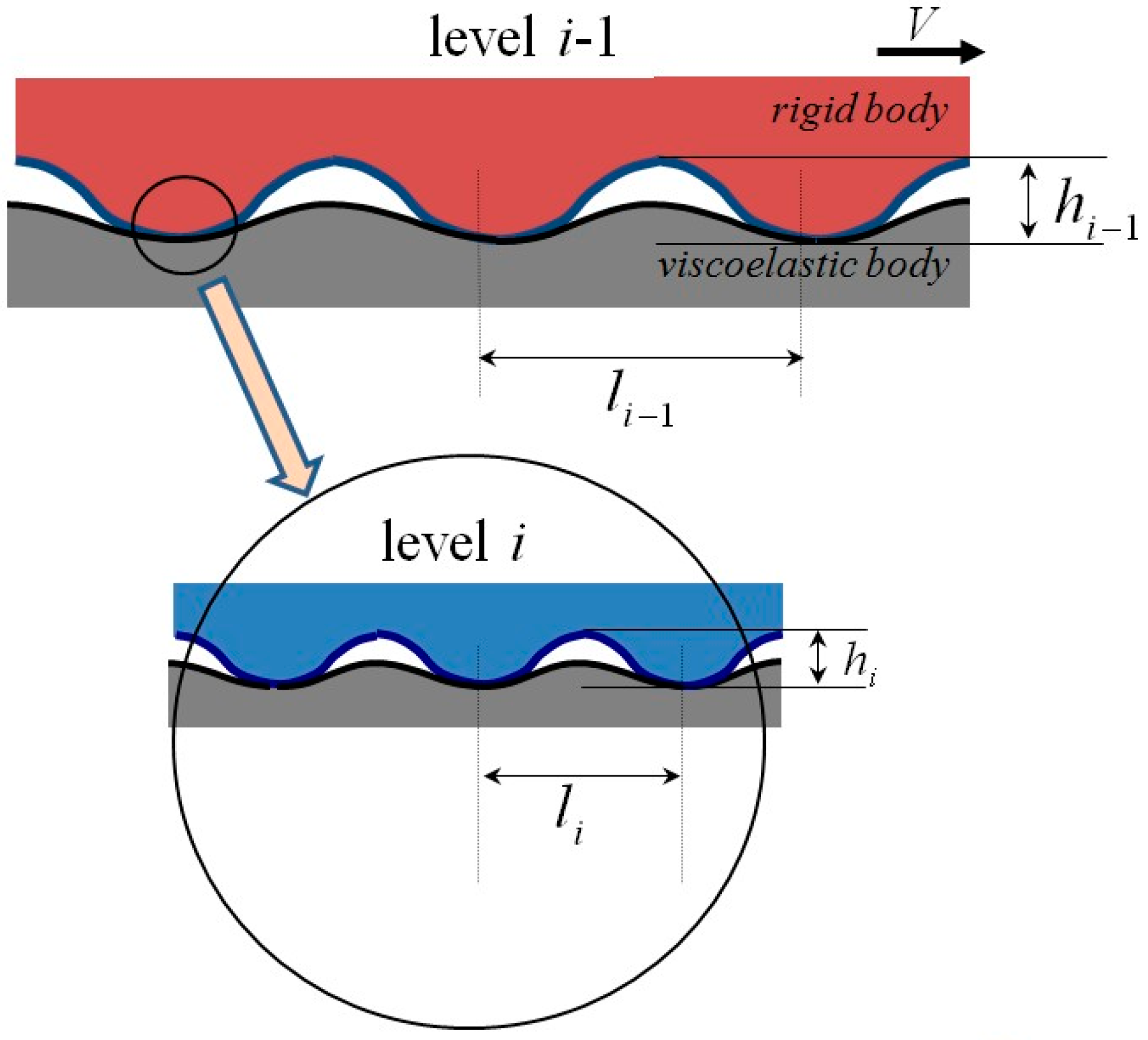
The rigid indenter is characterized by waviness at several scale levels described by a set of heights $h_i$ of asperities and distances $l_i$ between them, where $i=1\dots M$, $M$ is the number of the scale levels taken into account. Asperities of the i-th level are imposed on the surface of asperities of the (i − 1)-th level (Figure 1).

The rigid wavy surface slides over the surface of a viscoelastic foundation, the mechanical properties of which are described by the linear 1D model with one relaxation time:

$$w+T_{\epsilon }\frac{\partial w}{\partial t}=\frac{1}{K}\left(p+T_{\sigma }\frac{\partial p}{\partial t}\right),$$

(1)

where $p$ and $w$ are the normal pressure and displacement at the boundary of the viscoelastic foundation, $K$ is the elastic compliance of the viscoelastic foundation, $T_{\epsilon }$ and $T_{\sigma }$ are its retardation and relaxation times, respectively. The wavy surface slides with the constant velocity V.

Adhesion attraction acting between the surfaces is described by the Maugis-Dugdale model in which the adhesive stress $p_a$ is related to the gap $\delta$ by the equation [21]:

$$p_a(\delta )=\{\begin{array}{cc}{p}_0,& 0<\delta \le {\delta }_0\\ 0,& \delta >{\delta }_0\end{array},$$

(2)

where ${\delta }_0$ is the radius of action of the adhesion attraction. The specific energy of adhesion is then specified as:

$$\gamma ={\displaystyle {\int }_0^{+\infty }}\hspace{0.17em}{p}_a(\delta )d\delta =p_0{\delta }_0.$$

(3)

At each scale level, the contact problem for a periodic wavy indenter is solved. The friction force is calculated as a sum of two terms. The first term is due to hysteresis occurring when asperities at this scale level cyclically deform the viscoelastic foundation during sliding. The second term is the friction law determined from the solution of the contact problem at the inferior scale level. This law specifies the dependence of the tangential stress on the normal pressure at each point, it does not imply proportionality or any other imposed functional dependence between tangential and normal stress.

3. Contact Problem Solution at an i-th Scale Level

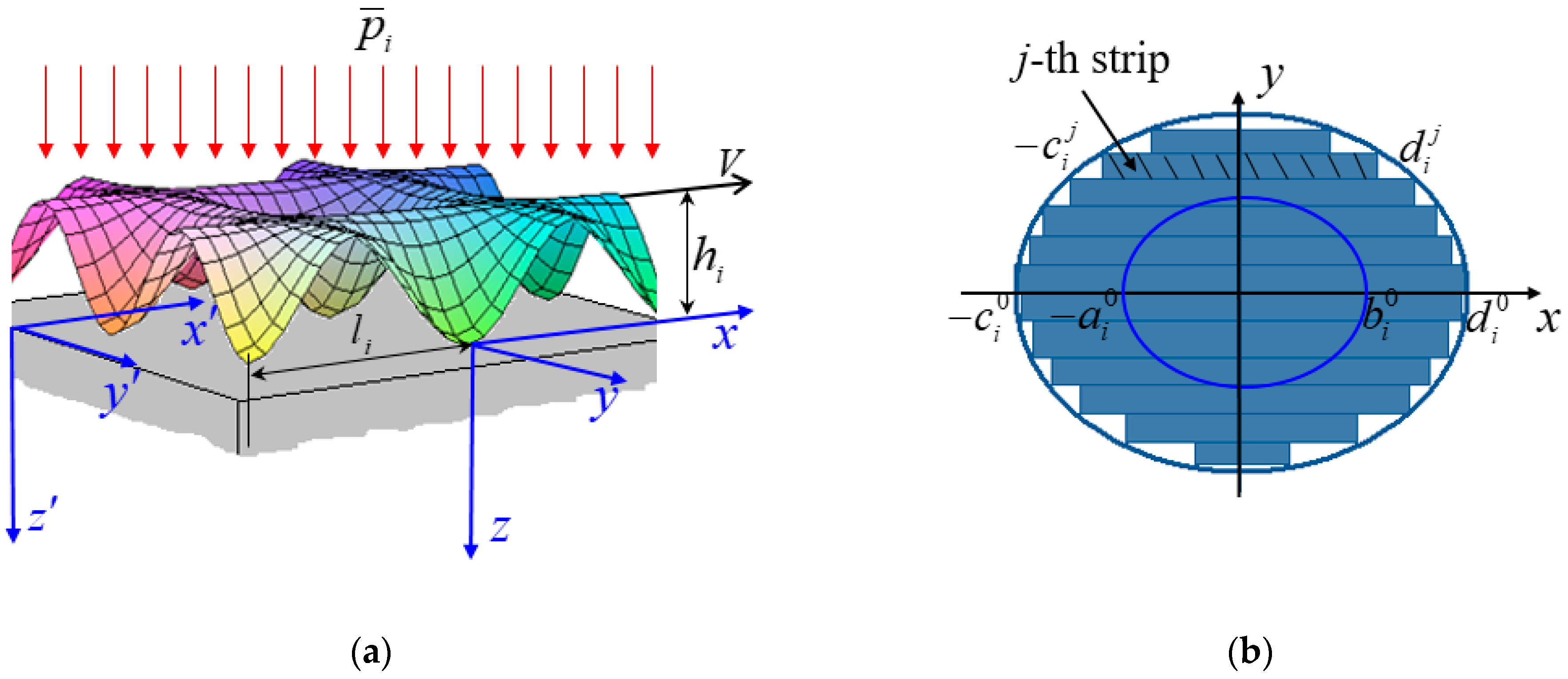
At an i-th scale level, the waviness of the surface is described by a function that is periodic in two directions (Figure 2a):

$$f_i\left(x,y\right)=h_i-\frac{h_i}{4}\left(\cos \left(\frac{2\pi x}{l_i}\right)+1\right)\left(\cos \left(\frac{2\pi y}{l_i}\right)+1\right).$$

(4)

Let us pass from the system of coordinates $(x^{\prime },y^{\prime },z^{\prime })$ attached to the viscoelastic base to the system of coordinates $(x,y,z)$ moving with the wavy surface with the constant velocity V. In the moving system, the stress and displacement do not depend explicitly on time, and Equation (1) for the i-th scale level takes the form:

$$w_i-V{T}_{\epsilon }\frac{\partial w_i}{\partial x}=\frac{1}{K}\left(p_i-T_{\sigma }V\frac{\partial p_i}{\partial x}\right).$$

(5)

In the moving system of coordinates, the boundary conditions for the stress and displacement of the viscoelastic foundation are the following

$$\begin{array}{ll}{w}_i(x,y)=f_i(x,y)+D_i,& (x,y)\in {\Omega }_i^c\\ p_i(x,y)=-p_0,& (x,y)\in {\Omega }_i^a\\ p_i(x,y)=0,& (x,y)\notin {\Omega }_i^c\cup {\Omega }_i^a\end{array}$$

(6)

where ${\Omega }_i^c$ and ${\Omega }_i^a$ are the contact and adhesion regions, respectively, $D_i$ is the maximum penetration of the wavy surface into the foundation at the i-th level. The equilibrium condition must be satisfied for the nominal pressure ${\overline{p}}_i$:

$${\overline{p}}_i=\frac{1}{l_i^2}{\displaystyle \underset{{\Omega }_i}{\iint }{p}_i(x,y)dx}dy,$$

(7)

where ${\Omega }_i={\Omega }_i^c\cup {\Omega }_i^a$ is the region of interaction at the i-th level.

The problem at the i-th scale level is solved by using the strip method. A cell of periodicity $x\in \left(-l_i/2,l_i/2\right)$, $y\in \left(-l_i/2,l_i/2\right)$ is divided into $2N$ strips of a thickness Δ parallel to the $x$-axis (Figure 2b). Penetration of the indenter into the j-th strip at the i-th scale level $D_i^j$ is given by the relation:

$$D_i^j=\frac{h_i}{2}\left(\cos \left(\frac{2\pi y_j}{l_i}\right)-1\right)+D_i.$$

(8)

Thus, the 3D contact problem is reduced to a 2D problem for each strip. The differential Equation (5) with Conditions (6), where $D_i^j$ defined by (8) is substituted instead of $D_i$, is solved analytically to obtain the closed form relation for the normal stress distribution. The regime of interaction in the gap should be appropriately chosen for each strip depending on the value of $D_i^j$—saturated contact, partial contact with saturated adhesion, partial contact with discrete regions of adhesion, or absence of contact. Detailed description of the method of solution of the 2D contact problem with different regimes of interaction is given in [17], and description of the strip method for the problem in question is given in [18,19].

As a result, the function of contact stress $p_i(x,y_j)$ is constructed analytically for each strip. The coordinates of the boundaries $-a_i^j,b_i^j$ of the contact region and $-c_i^j,d_i^j$ of the adhesion region are calculated numerically in each strip. After this, the contact area can be calculated as:

$$A_i=2\Delta {\displaystyle \sum _{j=1}^N(a_i^j+b_i^j)}.$$

(9)

When the distribution of the normal stress $p_i(x,y_j)$ is known for a j-th strip, the tangential stress can be calculated in accordance with the relation:

$${\tau }_i(x,y_j)=p_i(x,y_j)\frac{\partial f_i(x,y_j)}{\partial x}.$$

(10)

This stress is different from zero due to asymmetric distribution of the contact stress $p_i(x,y)$, which is due to viscous hysteresis in the material. The tangential stress ${\tau }_i(x,y)$ calculated in accordance with (10) is the hysteresis frictional stress. By averaging the obtained normal and tangential stresses over the cell of periodicity, we can calculate the mean (nominal) normal and tangential stress at the i-th scale level:

$${\overline{p}}_i=\frac{2\Delta }{l_i^2}{\displaystyle \sum _{j=1}^N{\displaystyle \underset{-l_i/2}{\overset{l_i/2}{\int }}{p}_i}(x,y_j)dx},\hspace{1em}{\overline{\tau }}_i=\frac{2\Delta }{l_i^2}{\displaystyle \sum _{j=1}^N{\displaystyle \underset{-l_i/2}{\overset{l_i/2}{\int }}{\tau }_i}(x,y_j)dx}.$$

(11)

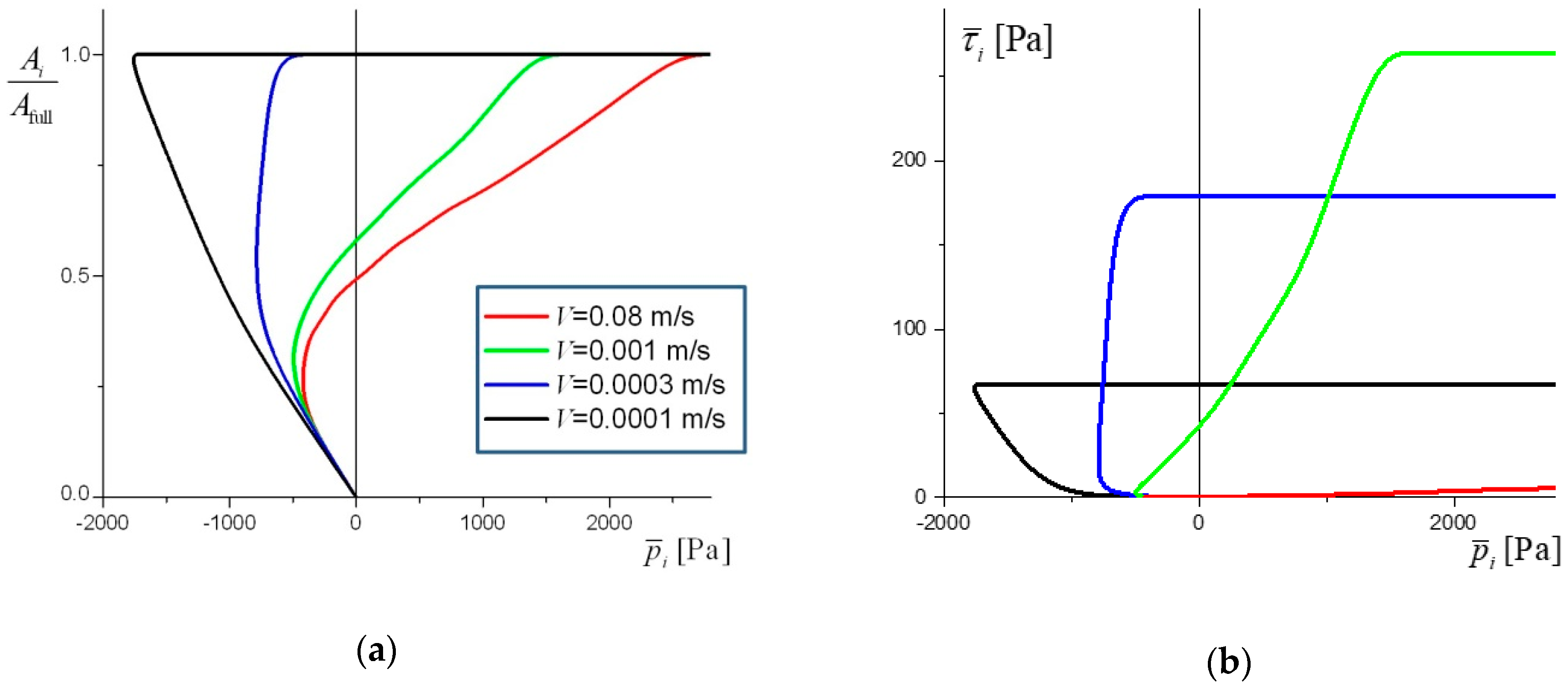
In Figure 3, examples of calculated results for an isolated scale level are presented. The ratio of the contact area $A_i$ to the full contact area $A_{\mathrm{full}}=l_i^2$ as a function of nominal stress is shown in Figure 3a. The mean frictional stress as a function of nominal stress is presented in Figure 3b.

The following input numerical values are used for the calculation. The mechanical properties of the viscoelastic foundation are taken: $K=1\hspace{0.17em}\mathrm{GPa}/\mathrm{m}$, $T_{\epsilon }=0.01\hspace{0.17em}\mathrm{s}$, $T_{\epsilon }/T_{\sigma }=100$. To clarify their physical meaning, note that Equation (1) describes a linear 1D viscoelastic body, e.g., a rubber layer of thickness $H=1\hspace{0.17em}\mathrm{mm}$ and elastic modulus $E=1\hspace{0.17em}\mathrm{MPa}$ lying on the rigid substrate, then its compliance is $K=E/H$. The geometric characteristics of the waviness are $l_i=500$ nm, $h_i=100$ nm. The adhesion is described by the parameters $\gamma =2.5\times {10}^{-5}\hspace{0.17em}\mathrm{N}/\mathrm{m}$, ${\delta }_0=10\hspace{0.17em}\mathrm{nm}$. The specific work of adhesion $\gamma$ corresponds to low-adhesive rubber, it is chosen so that to ensure both partial and full contact in the considered range of loads and velocities. The results are presented for various values of the sliding velocity V.

The results presented in Figure 3 show that both the contact area and frictional stress attain a constant value at some nominal pressure and remain constant when the pressure further increases. It is accounted for by the saturation of contact when the contact becomes full and the gap is zero over the entire contact surface. Taking into account adhesion attraction leads to the existence of contact at negative nominal pressures, which is more pronounced at lower velocities. Please note that the hysteresis friction force is positive (directed against the sliding direction) both for positive and for negative nominal stress.

The graphs presented in Figure 3b indicate that the friction force nonmonotonically depends on the velocity—it tends to zero at very high and very small velocities and attains maximum at some value of V. This behavior of the friction force is characteristic of the hysteresis friction of viscoelastic bodies [1,2,3,4]. Additionally, the graphs of the frictional stress versus nominal stress are ambiguous for some values of the velocity, e.g., for $V=0.1\hspace{0.17em}\mathrm{mm}/\mathrm{s}$. This ambiguity is caused by the combined effect of compliance and adhesion and it leads to a hysteresis in cyclic normal approach and separation of the surfaces, which is also the case for purely elastic bodies [22,23].

The function of frictional stress versus nominal pressure ${\overline{\tau }}_i={\overline{\tau }}_i[{\overline{p}}_i]$ constructed for the i-th level (examples of which are presented in Figure 3b) is used as a law of friction at the superior $(i-1)$-th scale level (see Figure 1). In the domain of ambiguity of the function ${\overline{\tau }}_i={\overline{\tau }}_i[{\overline{p}}_i]$, the upper part of the curve is used for calculation, which corresponds to the stable solution at unloading.

4. Constructing the Solution for a Multilevel Surface

In the case of $M$ scale levels, the solution is constructed as follows. At first, the Problem (5)–(7) is solved at the smallest M-th scale. From this solution, the law of friction ${\overline{\tau }}_M={\overline{\tau }}_M[{\overline{p}}_M]$ is constructed numerically by using Relations (10)–(11) for $i=M$. For the $(M-1)$-th level, the tangential stress is a sum two terms. The first term is due to hysteresis occurring when asperities of this scale level cyclically deform the viscoelastic foundation during sliding. The second term follows from the friction law determined at the M-th level, which is defined at each point by the normal stress $p_{M-1}(x,y_j)$:

$${\tau }_{M-1}=p_{M-1}(x,y_j)\frac{\partial }{\partial x}{f}_{M-1}(x,y_j)+{\overline{\tau }}_M\left[p_{M-1}(x,y_j)\right].$$

(12)

By averaging Equation (12) over the cell of periodicity $x\in \left(-l_i/2,l_i/2\right)$, $y\in \left(-l_i/2,l_i/2\right)$, we calculate the mean frictional stress of the $(M-1)$-th level:

$${\overline{\tau }}_{M-1}=\frac{2\Delta }{l_{M-1}^2}{\displaystyle \sum _{j=1}^N{\displaystyle \underset{-l_{M-1}/2}{\overset{l_{M-1}/2}{\int }}{p}_{M-1}(x,y_j)\frac{\partial }{\partial x}{f}_{M-1}(x,y_j)\hspace{0.17em}dx}}+\frac{2\Delta }{l_{M-1}^2}{\displaystyle \sum _{j=1}^N{\displaystyle \underset{-l_{M-1}/2}{\overset{l_{M-1}/2}{\int }}{\overline{\tau }}_M[p_{M-1}(x,y_j)]\hspace{0.17em}dx}},$$

(13)

whose dependence on the nominal pressure ${\overline{p}}_{M-1}$ will in turn serve as a law of friction for the $(M-2)$-th level: ${\overline{\tau }}_{M-1}={\overline{\tau }}_{M-1}[{\overline{p}}_{M-1}]$.

By subsequently repeating this procedure, we finally calculate the total coefficient of friction for the multilevel wavy surface:

$$\mu =\frac{{\overline{\tau }}_1}{{\overline{p}}_1}=\frac{2\Delta }{{\overline{p}}_1{l}_1^2}{\displaystyle \sum _{j=1}^N{\displaystyle \underset{-l_1/2}{\overset{l_1/2}{\int }}{p}_1(x,y_j)\frac{\partial }{\partial x}{f}_1(x,y_j)\hspace{0.17em}dx}}+\frac{2\Delta }{{\overline{p}}_1{l}_1^2}{\displaystyle \sum _{j=1}^N{\displaystyle \underset{-l_1/2}{\overset{l_1/2}{\int }}{\overline{\tau }}_2[p_1(x,y_j)]\hspace{0.17em}dx}}.$$

(14)

The first term of the right-hand side of Equation (14) is the contribution of the asperities of the first (largest) scale level into the hysteresis friction force. The second term is the contribution of the second and all the subsequent scale levels up to the M-th one.

In the general case, the solution of the multilevel problem requires the contact problem to be subsequently solved at each scale level. The most difficult part of the solution is the determination of the boundaries $-a_i^j, b_i^j$ of the contact region and the boundaries $-c_i^j, d_i^j$ of the adhesion region in a cell of periodicity for each scale level i and each number j of the strip, which includes the determination of the regime of filling of the gap in each strip. These values are determined by numerically solving a system of two to four algebraic equations by means of the Maple software (Maplesoft, Waterloo, ON, Canada).

In the particular case, where the external load and adhesion are high enough so that the saturated contact occurs at all scale levels, the solution is significantly simplified. The pressure distribution at each scale level is then specified by a simple analytic relation in a cell of periodicity $x\in \left(-l_i/2,l_i/2\right)$, $y\in \left(-l_i/2,l_i/2\right)$:

$$\begin{array}{ll}{p}_i(x,y_j)& =\frac{K}{2(l_i^2+4{\pi }^2{T}_{\sigma }^2{V}^2)}[\frac{h_i}{2}\left(\cos \frac{2\pi y_j}{l_i}+1\right)\\ & \times \left\{(l_i^2+4{\pi }^2{T}_{\epsilon }{T}_{\sigma }{V}^2)\cos \frac{2\pi x}{l_i}+2\pi l_{i}V(T_{\epsilon }-T_{\sigma })\sin \frac{2\pi x}{l_i}\right\}\\ & +(4{\pi }^2{T}_{\sigma }^2{V}^2+l_i^2)\left\{\frac{h_i}{2}\left(\cos \frac{2\pi y_j}{l_i}-3\right)+2D\right\}].\end{array}$$

(15)

After substituting Relation (15) into Equations (10) and (11), the relation for the frictional stress ${\overline{\tau }}_i$ independent of the nominal pressure ${\overline{p}}_i$ is obtained. Thus, the law of friction is reduced to a constant value of the friction force which is calculated at each scale level independently from other levels. This allows one to calculate the total friction force by direct summation of contributions of all scale levels. As a result, the total coefficient of friction has the form:

$$\mu =\frac{{\pi }^{2}KV(T_{\epsilon }-T_{\sigma })}{{\overline{p}}_1}{\displaystyle \sum _{i=1}^N\frac{h_i}{4{\pi }^2{V}^2{T}_{\sigma }^2+l_i^2}}.$$

(16)

where ${\overline{p}}_1$ is the external nominal pressure which coincides with the nominal pressure at the first level.

5. Results of Calculation for a Two-Level Surface

Calculation is carried out for a two-level surface with the waviness parameters l₁ = 10 μm, h₁ = 1 μm, l₂ = 500 nm, h₂ = 100 nm. The values are chosen so that the smaller scale has a “sharper” waviness, and its contribution to the total friction force is larger. This can model a situation where the contact has two distinct scales—e.g., some waviness at which smaller roughness is applied. The properties of the viscoelastic foundation and adhesion parameters are the same as for the results presented in Figure 3. The external nominal pressure is 0.1 kPa, the sliding velocity ranges from 0 to 0.1 m/s.

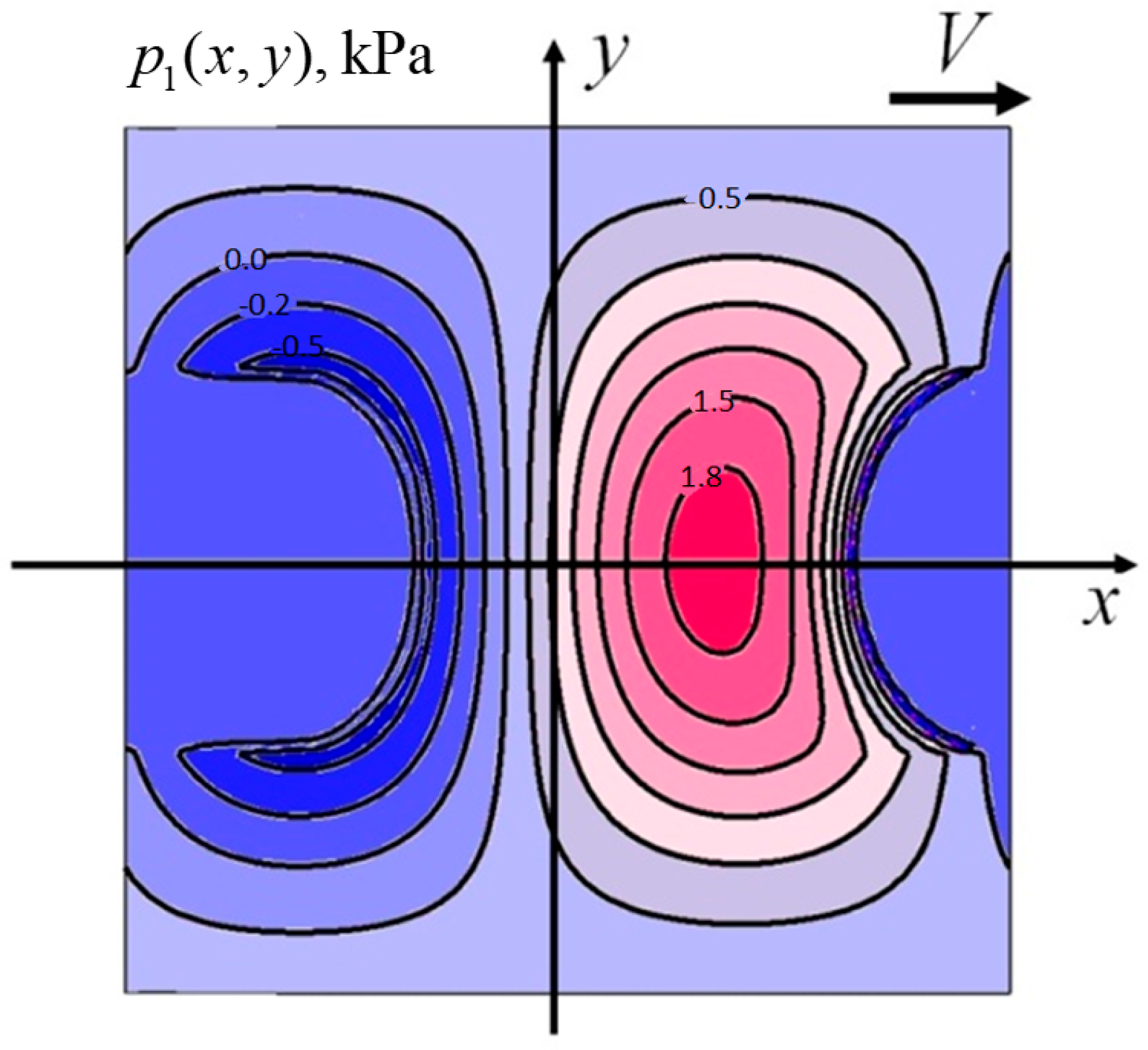
In Figure 4, the map of normal contact stress p₁(x, y) is shown for the 1st scale level at the velocity V = 0.005 m/s. The map is constructed in the cell of periodicity x ∈ (−l₁/2, l₁/2), y ∈ (−l₁/2, l₁/2). The red spot corresponds to the highest normal stress, dark blue to the adhesion regions where the pressure is negative. The distribution of the stress p₁(x, y) is nonsymmetric with respect to the y-axis, the maximum being shifted in the direction of sliding, which is due to the viscous properties of the foundation.

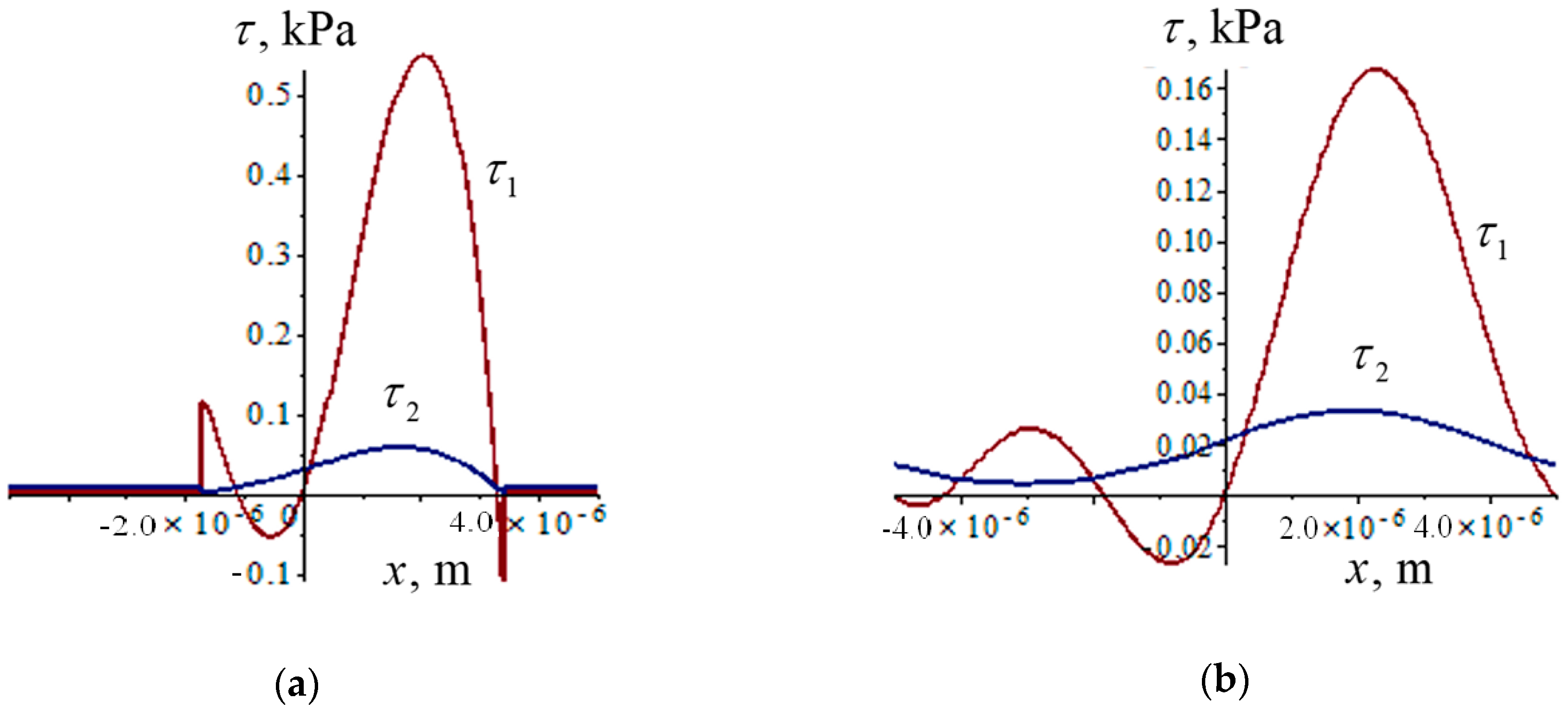
Figure 5 illustrates the contribution of the tangential stresses from two scale level, τ₁(x, y) and τ₂(x, y) at the same velocity V = 0.005 m/s. The results are shown as functions of x ∈ (−l₁/2, l₁/2) in the strips j = 0 and j = 63. The number of strips in a half-period is taken N = 100 for the calculation. For j = 0, i.e., in the central section, the contact is partial and the adhesion acts in discrete intervals with respect to x. There are regions in which τ₁ = τ₂ = 0. For j = 63, the contact is saturated. For this value of velocity, the contribution of the 1st level is more significant than the contribution of the 2nd one.

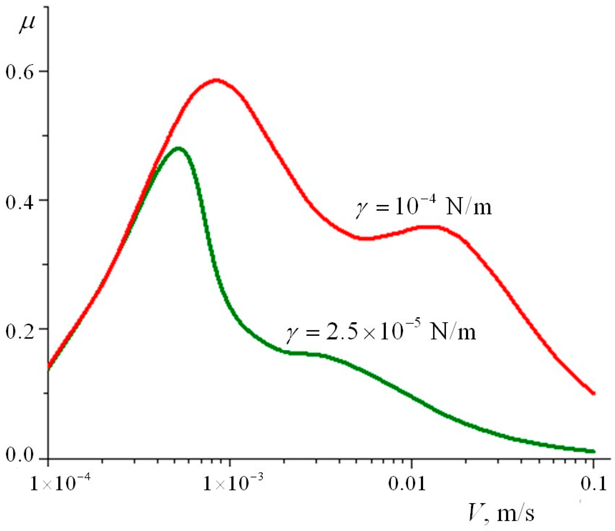
However, for lower values of the sliding velocity, the contribution of the 2nd scale level becomes more considerable. This can be seen in Figure 6 which depicts the total friction coefficient for the two-level surface as a function of the sliding velocity for two values of the specific energy of adhesion. The right peak corresponds to the contribution of the first scale level, the left peak to the second level.

6. Discussion

The results obtained show that depending on the values of waviness parameters, the coefficient of friction as a function of sliding velocity can have several peaks, each being associated with hysteretic losses at some scale level. It was first observed by Grosch that the master curve of rubber friction can have more than one peak [1]. He concluded that in the general case, the master curve has two peaks due to the two mechanisms of rubber friction—adhesion and hysteretic losses. Master curves with two peaks were also experimentally obtained in [24,25] and by numerical modeling in [7]. The possibility of observing several peaks corresponding to resonance frequencies due to different mechanisms of energy loss was pointed out by Persson [26]. In the present study, a phenomenological law of friction is obtained from considering the contribution of lower scale levels, including both hysteretic losses and adhesion forces acting in the direction normal to the surface. In this case, it is impossible to say that one peak is due to adhesion and the other is due to hysteresis, for both peaks in Figure 6 are due to hysteretic resonance, and both are strongly influenced by adhesion.

The graphs shown in Figure 6 allow one to conclude that increasing the specific energy of adhesion not only increases the coefficient of friction, but also shifts the peaks in the direction of higher velocities.

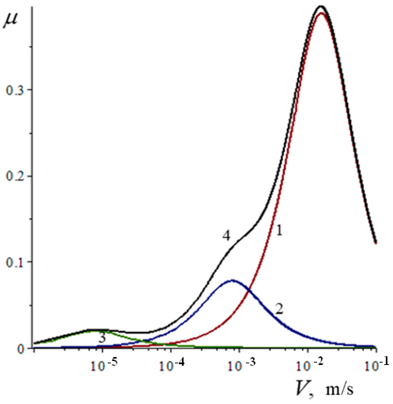
Please note that the model presented takes into account not only partial contact but also partial regions of adhesion. When the contact is assumed to be complete at all scale levels, the calculation of the friction force is significantly simplified (see Equation (16)). In Figure 7, the graph of the coefficient of friction as a function of velocity is presented for the case where the external nominal pressure is high enough to ensure saturated contact at all three scale levels that are taken into account. These scale levels have the following geometrical characteristics: l₁ = 10 μm, h₁ = 1 μm, l₂ = 500 nm, h₂ = 100 nm, l₃ = 5 nm, h₃ = 5 nm, . The nominal pressure is ${\overline{p}}_1$ = 5 MPa. All the remaining parameters coincide with those used for calculating the results presented in Figure 6. Curves 1, 2, and 3 correspond to contributions of the first, second, and third scale levels, respectively. Curve 4 corresponds to the total coefficient of friction, which is, in this case, a direct sum of the three components.

The results show that the peak associated with the largest (1st) scale level is the highest, whereas the 2nd and 3rd levels give significantly smaller peaks. By comparing the results presented in Figure 6 with those of Figure 7, one can conclude that neglecting partial character of contact and adhesion interaction can lead to substantial underestimation of the contribution of smaller scale levels into the total friction force.

7. Conclusions

The sliding friction between a multilevel wavy surface and a viscoelastic foundation is theoretically modeled in dry conditions. The method is suggested to calculate the friction force due to hysteretic losses in the viscoelastic material and adhesion forces acting between the surfaces taking into account the possibility of different contact regimes (partial contact with partial or full adhesion or full contact) at each scale levels. The method is based on determining the law of friction at each scale from examination the interaction at inferior scales. The calculation is performed for a two-level wavy surface. In the particular case of full contact at all scale levels, the analytic solution is obtained. It is found that the coefficient of friction as a function of sliding velocity can have more than one peaks, each associated with a certain scale level.

References

- Grosch, K.A. The relation between the friction and visco-elastic properties of rubber. Proc. R. Soc. Lond. Ser. A 1963, 274, 21–39. [Google Scholar] [CrossRef]
- Christensen, R.M. Theory of Viscoelasticity, 2nd ed.; Academic Press: New York, NY, USA, 1982; ISBN 978-0-12-174252-2. [Google Scholar]
- Klüppel, M.; Heinrich, G. Rubber friction on self-affine road tracks. Rubber Chem. Technol. 2000, 73, 578–606. [Google Scholar] [CrossRef]
- Persson, B.N.J. Theory of rubber friction and contact mechanics. J. Chem. Phys. 2001, 115, 3840–3861. [Google Scholar] [CrossRef] [Green Version]
- Li, Q.; Popov, M.; Dimaki, A.; Filippov, A.E.; Kürschner, S.; Popov, V.L. Friction between a viscoelastic body and a rigid surface with random self-affine roughness. Phys. Rev. Lett. 2013, 111, 034301. [Google Scholar] [CrossRef] [PubMed]
- Ciavarella, M. A simplified version of Persson’s multiscale theory for rubber friction due to viscoelastic losses. J. Tribol. 2017, 140, 011403. [Google Scholar] [CrossRef]
- Nettingsmeier, J.; Wriggers, P. Frictional contact of elastomer materials on rough rigid surfaces. PAMM Proc. Appl. Math. Mech. 2004, 4, 360–361. [Google Scholar] [CrossRef]
- Carbone, G.; Putignano, C. Rough viscoelastic sliding contact: Theory and experiments. Phys. Rev. 2014, E89, 032408. [Google Scholar] [CrossRef] [PubMed]
- Scaraggi, M.; Persson, B.N.J. Friction and universal contact area law for randomly rough viscoelastic contacts. J. Phys. Condens. Matter 2015, 27, 105102. [Google Scholar] [CrossRef] [PubMed]
- Menga, N.; Afferrante, L.; Demelio, G.P.; Carbone, G. Rough contact of sliding viscoelastic layers: Numerical calculations and theoretical predictions. Tribol. Int. 2018, 122, 67–75. [Google Scholar] [CrossRef]
- Tsukanov, I.Y. Partial contact of a rigid multisinusoidal wavy surface with an elastic half-plane. Adv. Tribol. 2018, 8431467. [Google Scholar] [CrossRef]
- Goryacheva, I.G.; Sadeghi, F. Contact Characteristics of a Rolling/Sliding Cylinder and a Viscoelastic Layer Bonded to an Elastic Substrate. Wear 1995, 184, 125–132. [Google Scholar] [CrossRef]
- Goryacheva, I.G. Contact Mechanics in Tribology; Kluwer Academic Publ: Dordercht, The Netherlands, 1998; ISBN 978-0-7923-5257-0. [Google Scholar]
- Menga, N.; Putignano, C.; Carbone, G.; Demelio, G.P. The sliding contact of a rigid wavy surface with a viscoelastic half-space. Proc. R. Soc. A 2014, 470. [Google Scholar] [CrossRef]
- Sheptunov, B.V.; Goryacheva, I.G.; Nozdrin, M.A. Contact problem of die regular relief motion over viscoelastic base. J. Frict. Wear 2013, 34, 83–91. [Google Scholar] [CrossRef]
- Goryacheva, I.G.; Stepanov, F.I.; Torskaya, E.V. Effect of Friction in Sliding Contact of a Sphere over a Viscoelastic Half-Space. In Mathematical Modeling and Optimization of Complex Structures; Neittaanmäki, P., Repin, S., Tuovinen, T., Eds.; Springer: Berlin, Germany, 2016; pp. 93–104. [Google Scholar] [CrossRef]
- Goryacheva, I.G.; Makhovskaya, Y.Y. Modeling of friction at different scale levels. Mech. Solids 2010, 45, 390–398. [Google Scholar] [CrossRef]
- Goryacheva, I.G.; Makhovskaya, Y.Y. Sliding of a wavy indenter on a viscoelastic layer surface in the case of adhesion. Mech. Solids 2015, 50, 439–450. [Google Scholar] [CrossRef]
- Goryacheva, I.; Makhovskaya, Y. Adhesion effect in sliding of a periodic surface and an individual indenter upon a viscoelastic base. J. Strain Anal. Eng. Des. 2016, 51, 286–293. [Google Scholar] [CrossRef]
- Morozov, A.V.; Makhovskaya, Y.Y. Effect of adhesion properties of frost-resistant rubbers on sliding friction. In Proceedings of the 4th International Conference on Industrial Engineering; Radionov, A.A., Kravchenko, O.A., Guzeev, V.I., Rozhdestvenskiy, Y.V., Eds.; Springer: Basel, Switzerland, 2019; pp. 1029–1037. [Google Scholar] [CrossRef]
- Maugis, D. Adhesion of spheres: The JKR-DMT transition using a Dugdale model. J. Colloid Interface Sci. 1991, 150, 243–269. [Google Scholar] [CrossRef]
- Greenwood, J.A. Adhesion of elastic spheres. Proc. R. Soc. Lond. A 1997, 453, 1277–1297. [Google Scholar] [CrossRef]
- Johnson, K.L. Mechanics of adhesion. Tribol. Int. 1998, 31, 413. [Google Scholar] [CrossRef]
- Moor, D.F. Friction and wear in rubbers and tyres. Wear 1980, 61, 273–282. [Google Scholar] [CrossRef]
- Morozov, A.V. Experimental study of the influence of rubber properties on sliding friction in dry contact. In Proceedings of the International Conference BALTTRIB’2017, Kaunas, Lithuania, 16–17 November 2017; Lithuanian Scientific Society Department “Tribologija” Aleksandras Stulginskis University: Kaunas, Lithuania, 2017; pp. 135–139. [Google Scholar] [CrossRef]
- Persson, B.N.J. Sliding Friction: Physical Principles and Applications; Springer: Heidelberg, Germany, 1998; ISBN 978-3-540-67192-3. [Google Scholar]
Figure 1.
Scheme of contact of the multilevel wavy surface and a viscoelastic body at two levels.
Figure 2.
Schemes illustrating the formulation and solution of the problem at the i-th scale level: (a) Scheme of contact at the i-th level; (b) Scheme of using the strip method of solution.
Figure 3.
Results of the contact problem solution at a separate scale level: (a) Contact area ratio vs. nominal pressure; (b) Mean frictional stress vs. nominal pressure.
Figure 4.
Distribution of the normal stress in a cell of periodicity at the 1st level.
Figure 5.
Distributions of the tangential stress contributed from two scale levels: (a) for j = 0; (b) for j = 63.
Figure 6.
Results of calculation for the two-level problem: the coefficient of friction as a function of sliding velocity.
Figure 7.
The coefficient of friction as a function of velocity for the case of full contact.
© 2019 by the author. Licensee MDPI, Basel, Switzerland. This article is an open access article distributed under the terms and conditions of the Creative Commons Attribution (CC BY) license (http://creativecommons.org/licenses/by/4.0/).
Share and Cite
MDPI and ACS Style
Makhovskaya, Y. Modeling Sliding Friction of a Multiscale Wavy Surface over a Viscoelastic Foundation Taking into Account Adhesion. Lubricants 2019, 7, 13. https://doi.org/10.3390/lubricants7020013
AMA Style
Makhovskaya Y. Modeling Sliding Friction of a Multiscale Wavy Surface over a Viscoelastic Foundation Taking into Account Adhesion. Lubricants. 2019; 7(2):13. https://doi.org/10.3390/lubricants7020013
Chicago/Turabian StyleMakhovskaya, Yulia. 2019. "Modeling Sliding Friction of a Multiscale Wavy Surface over a Viscoelastic Foundation Taking into Account Adhesion" Lubricants 7, no. 2: 13. https://doi.org/10.3390/lubricants7020013
Note that from the first issue of 2016, this journal uses article numbers instead of page numbers. See further details here.