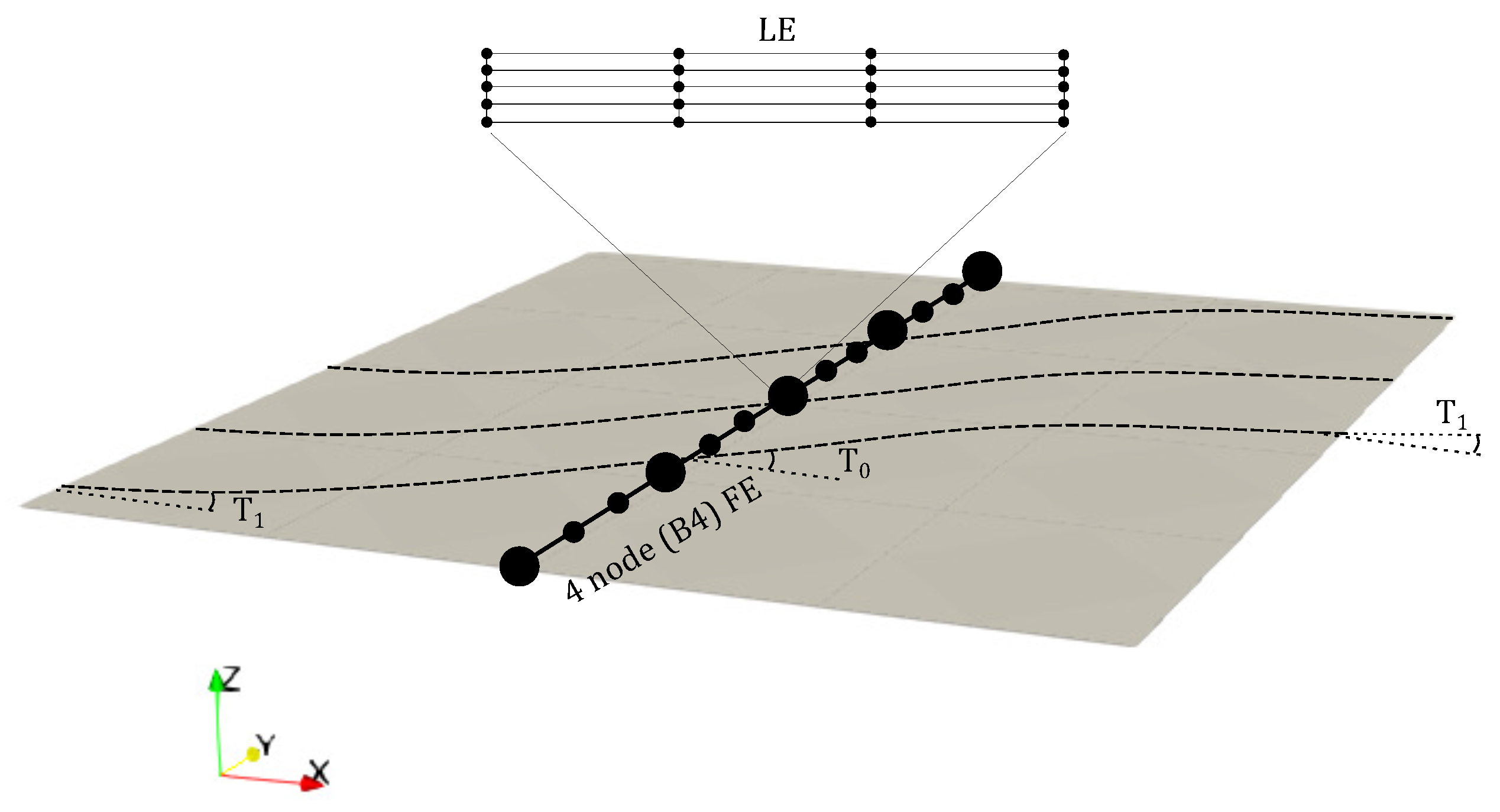
Figure 1.
Representation of the finite element (FE) and Lagrange expansion (LE) theories employed over the macroscale structure. FE are used along the longitudinal axis and LE are utilised for the cross-section. and represent the fibre orientation at the centre of the plate and at the edge, respectively.
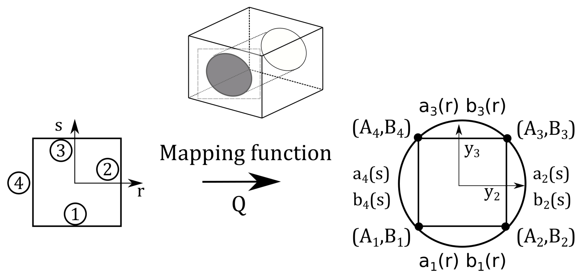
Figure 2.
Mapping of the fibre section of the RUC by means of the blending function method. Reprinted from Reference [
42], with permission from Elsevier.
Figure 2.
Mapping of the fibre section of the RUC by means of the blending function method. Reprinted from Reference [
42], with permission from Elsevier.
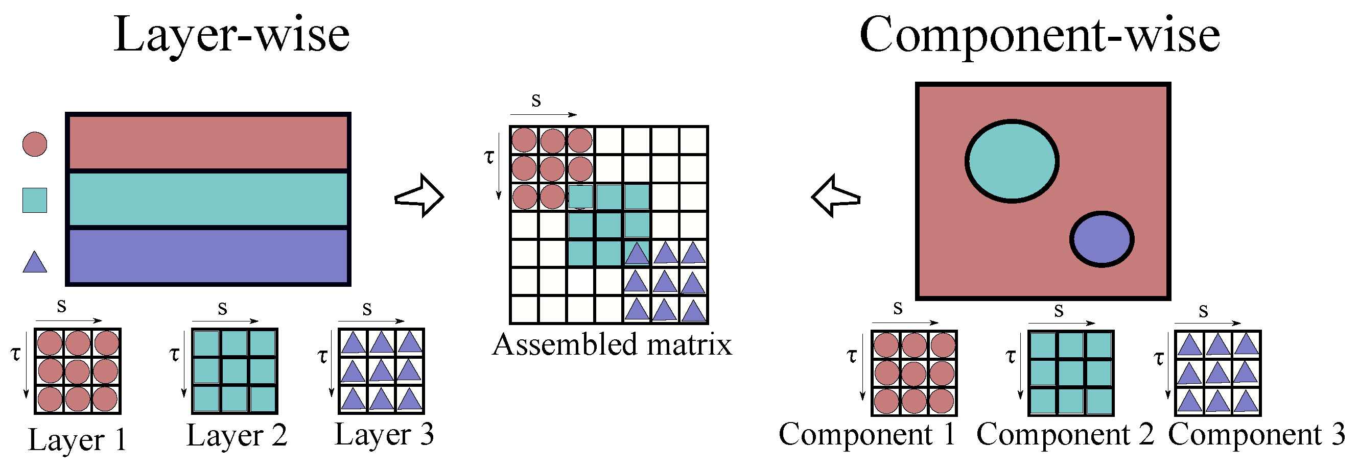
Figure 3.
Layer-wise and component-wise assembly procedures.
Figure 3.
Layer-wise and component-wise assembly procedures.
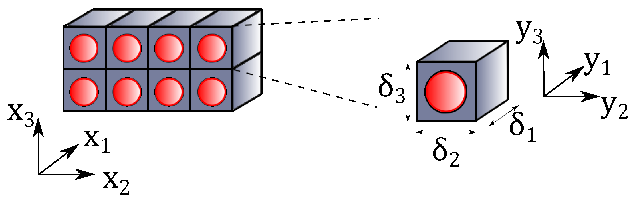
Figure 4.
Representation of a periodic heterogeneous material and its RUC along with the global and local coordinate reference frames.
Figure 4.
Representation of a periodic heterogeneous material and its RUC along with the global and local coordinate reference frames.
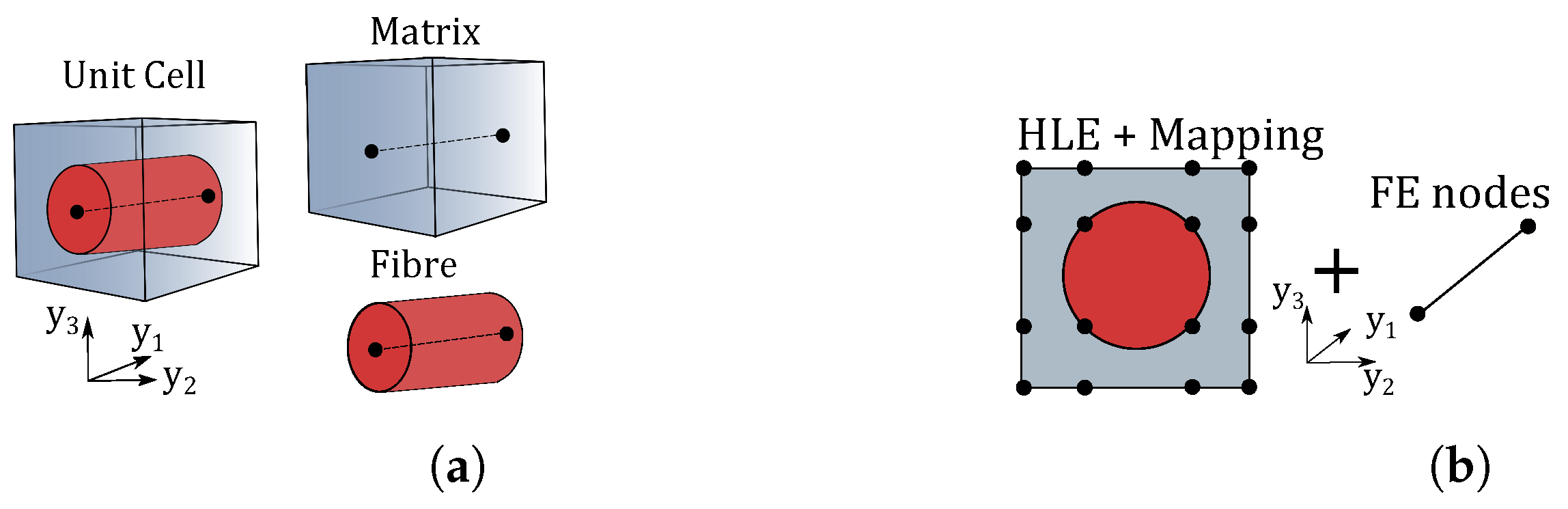
Figure 5.
(a) Component-wise modelling of composite microstructure with different phases. (b) Kinematics used to define the RUC cross-section.
Figure 5.
(a) Component-wise modelling of composite microstructure with different phases. (b) Kinematics used to define the RUC cross-section.
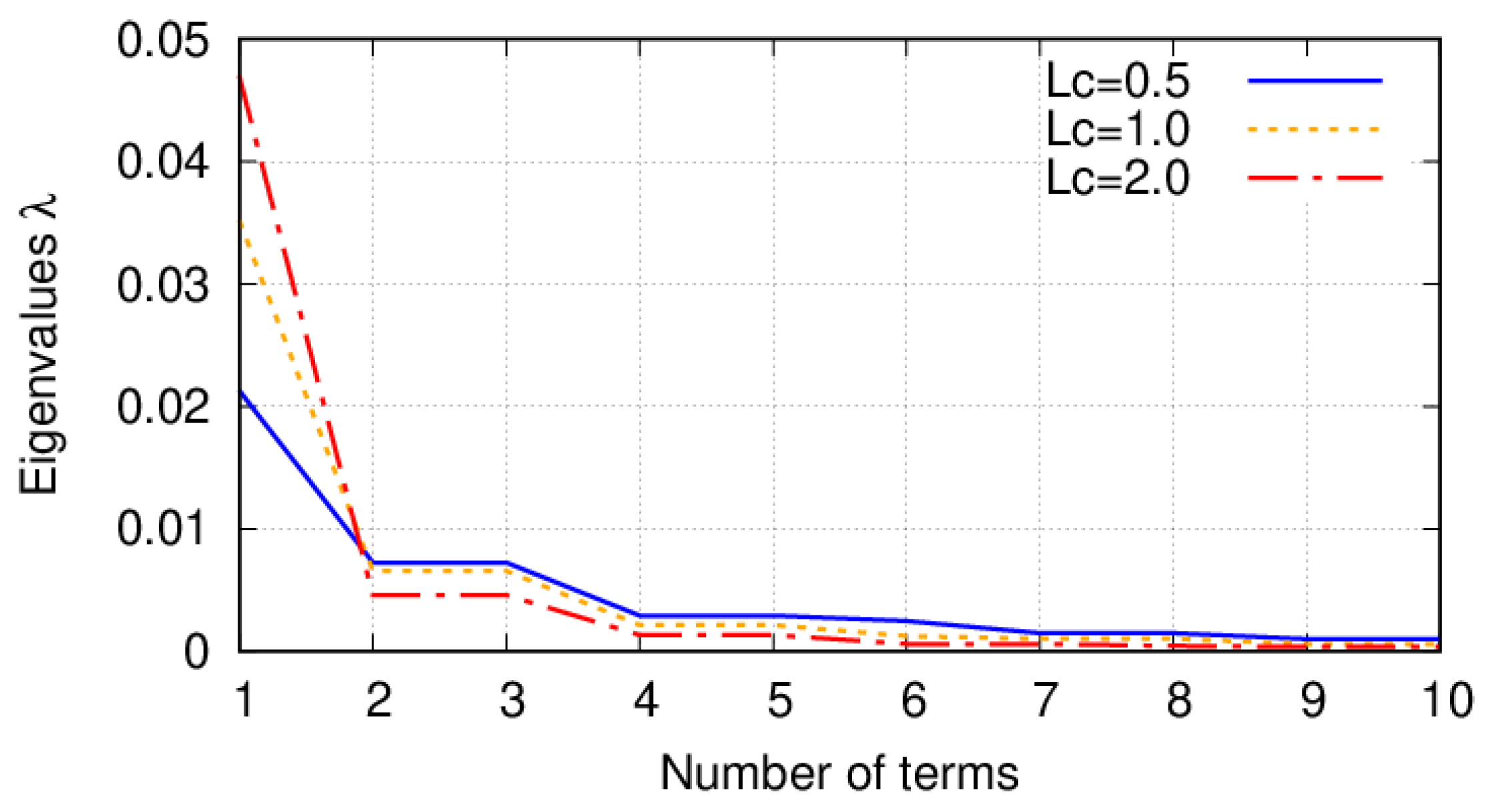
Figure 6.
Eigenvalues of the Fredholm integral for different correlation lengths.
Figure 6.
Eigenvalues of the Fredholm integral for different correlation lengths.
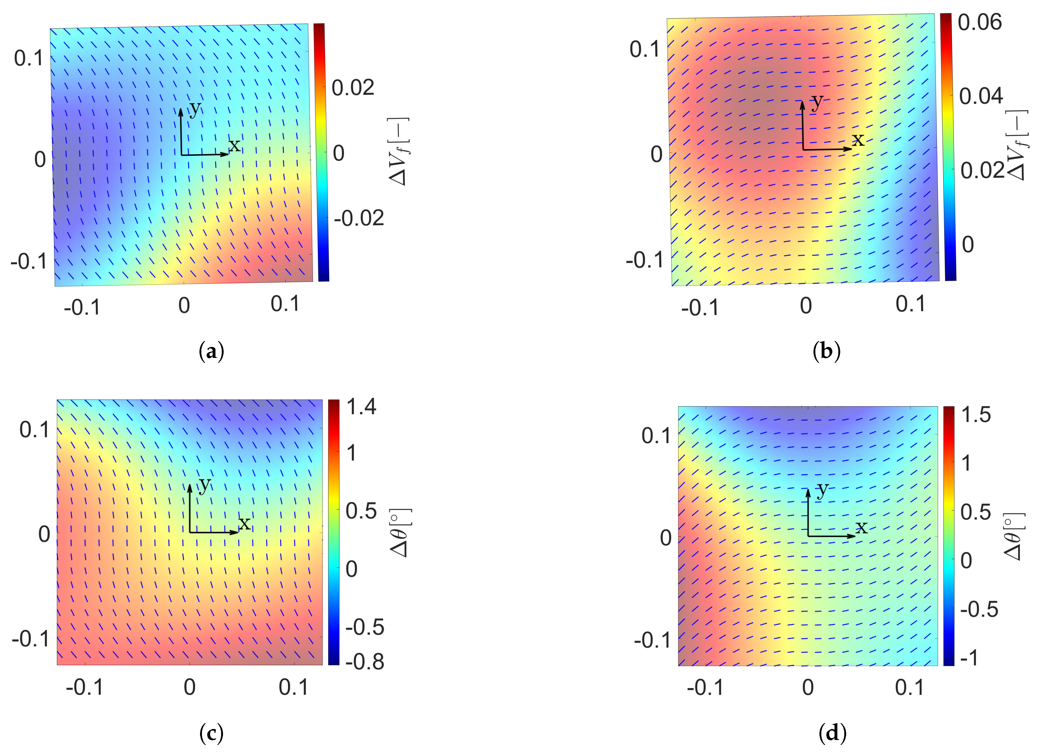
Figure 7.
(a) Fibre volume fraction () random field over a . (b) random field over a ply. (c) Misalignment field over a ply. (d) Misalignment field over a ply. These random fields are generated by means of the Karhunen-Loève expansion. The stochastic fields represent the fibre volume fraction and has a mean value and a standard deviation and fibre misalignments of null mean and standard deviation .
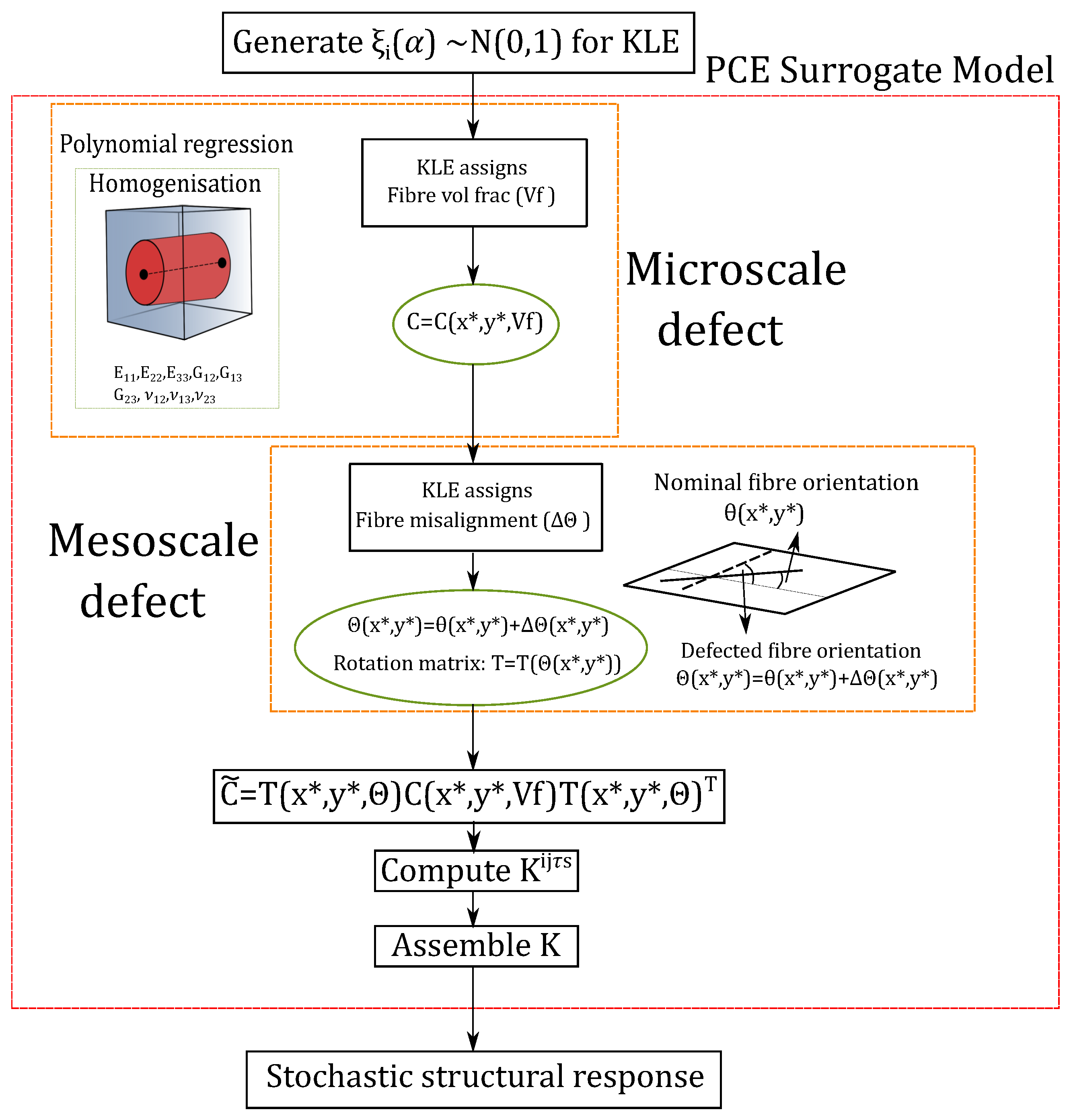
Figure 8.
Flow-chart of the stochastic structural analysis performed.
Figure 8.
Flow-chart of the stochastic structural analysis performed.
Figure 9.
(a) vs. , (b) vs. , (c) vs. , (d) vs. , (e) vs. , (f) vs. . Sampling results and data fit of the homogenised material properties. Fibre volume fraction is treated as a Gaussian random variable with mean value and standard deviation .
Figure 9.
(a) vs. , (b) vs. , (c) vs. , (d) vs. , (e) vs. , (f) vs. . Sampling results and data fit of the homogenised material properties. Fibre volume fraction is treated as a Gaussian random variable with mean value and standard deviation .
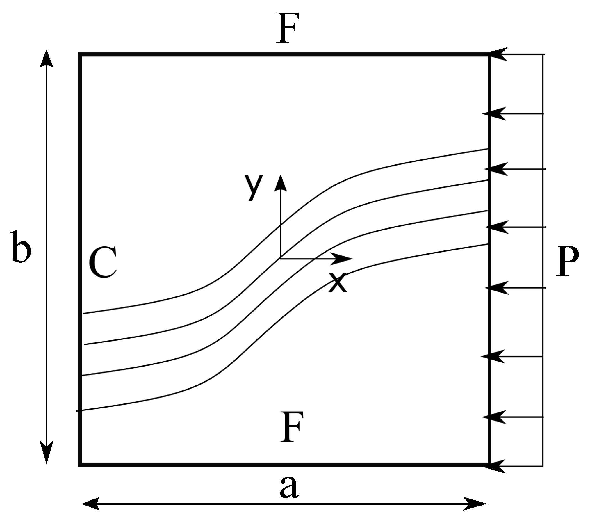
Figure 10.
Boundary conditions of the laminated plates. C and F stand for clamped and free edges respectively. Pressure P is exerted uniformly on the laminate yz plane.
Figure 10.
Boundary conditions of the laminated plates. C and F stand for clamped and free edges respectively. Pressure P is exerted uniformly on the laminate yz plane.
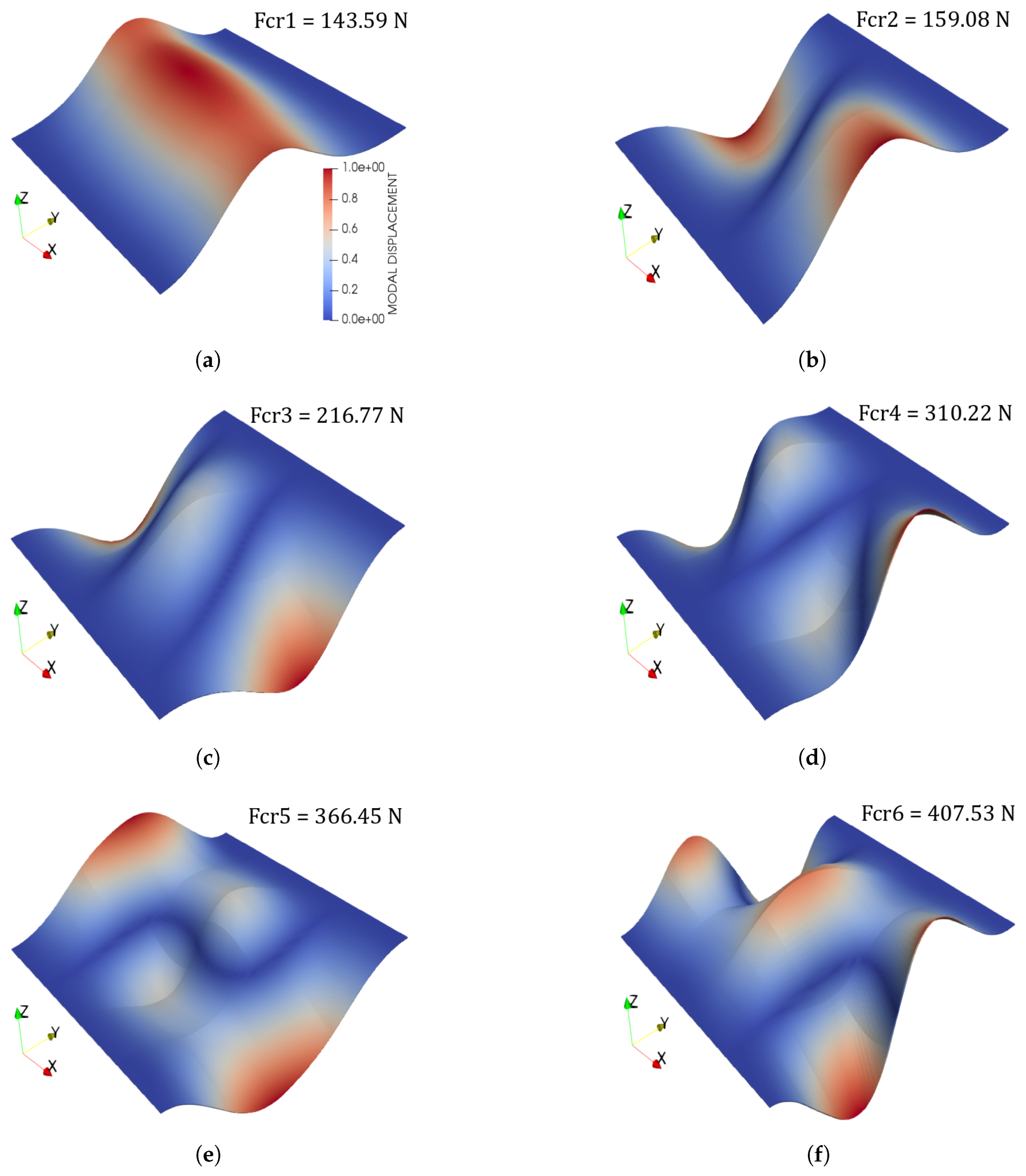
Figure 11.
(a) First mode, (b) Second mode, (c) Third mode, (d) Fourth mode, (e) Fifth mode, (f) Sixth mode. Case 1 pristine buckling modes. A uniform fibre volume is considered and no fibre waviness. The colour bar in (a) applies for all figures in this panel.
Figure 11.
(a) First mode, (b) Second mode, (c) Third mode, (d) Fourth mode, (e) Fifth mode, (f) Sixth mode. Case 1 pristine buckling modes. A uniform fibre volume is considered and no fibre waviness. The colour bar in (a) applies for all figures in this panel.
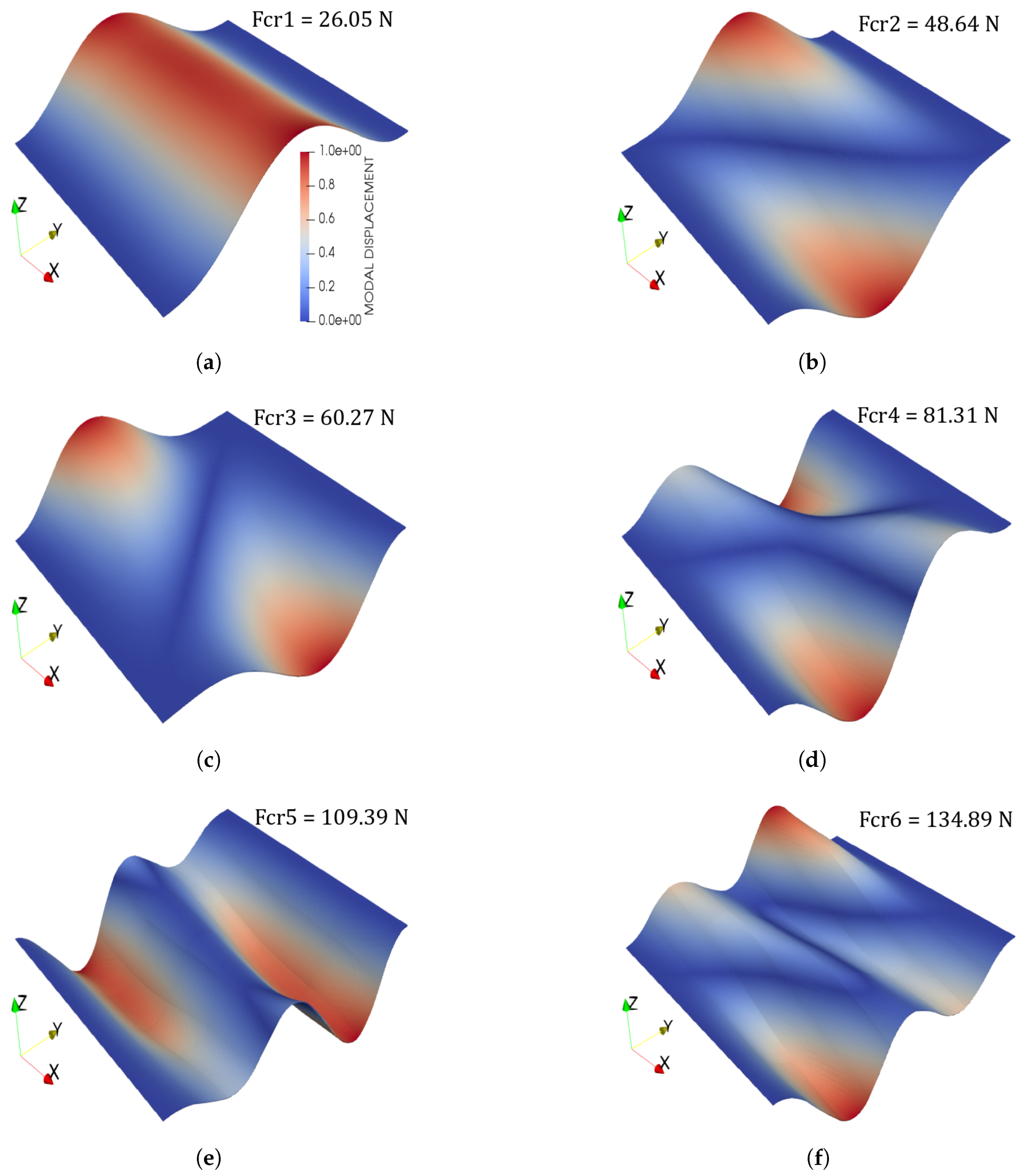
Figure 12.
(a) First mode, (b) Second mode, (c) Third mode, (d) Fourth mode, (e) Fifth mode, (f) Sixth mode. Case 2 pristine buckling modes. A uniform fibre volume is considered and no fibre waviness. The colour bar in (a) applies for all figures in this panel.
Figure 12.
(a) First mode, (b) Second mode, (c) Third mode, (d) Fourth mode, (e) Fifth mode, (f) Sixth mode. Case 2 pristine buckling modes. A uniform fibre volume is considered and no fibre waviness. The colour bar in (a) applies for all figures in this panel.
Figure 13.
(a) Case 1 , (b) Case 2 . Mean value and COV convergence of the Case 1 and Case 2 buckling loads provided by the computed PCE for different amount of samples. Fibre volume fraction is treated as a Gaussian random variable with mean value and standard deviation and no fibre waviness.
Figure 13.
(a) Case 1 , (b) Case 2 . Mean value and COV convergence of the Case 1 and Case 2 buckling loads provided by the computed PCE for different amount of samples. Fibre volume fraction is treated as a Gaussian random variable with mean value and standard deviation and no fibre waviness.
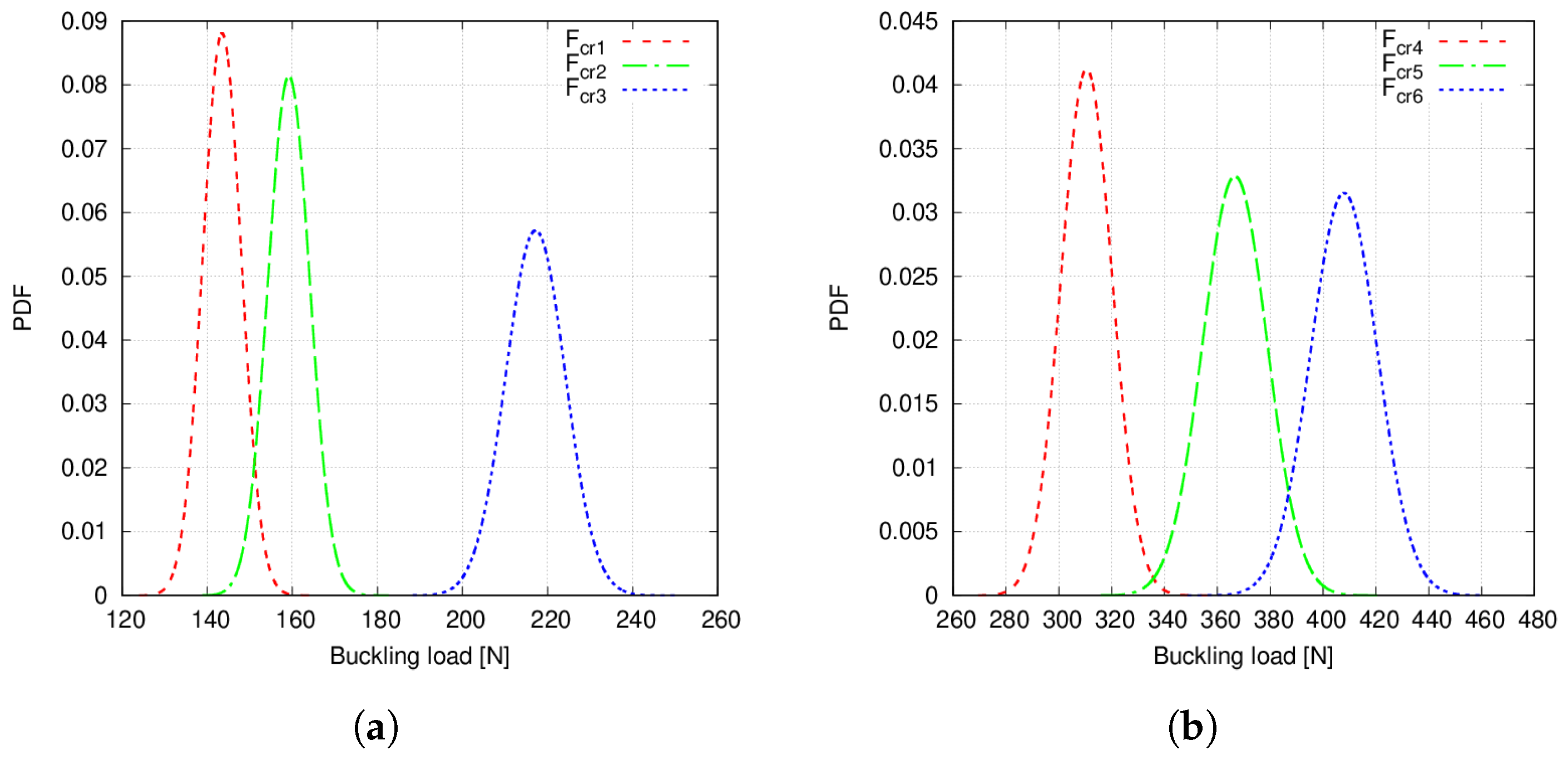
Figure 14.
(a) Case 1 , and PDFs, (b) Case 1 , and PDFs. Fibre volume fraction is treated as a Gaussian random variable with mean value and standard deviation and no fibre waviness.
Figure 14.
(a) Case 1 , and PDFs, (b) Case 1 , and PDFs. Fibre volume fraction is treated as a Gaussian random variable with mean value and standard deviation and no fibre waviness.
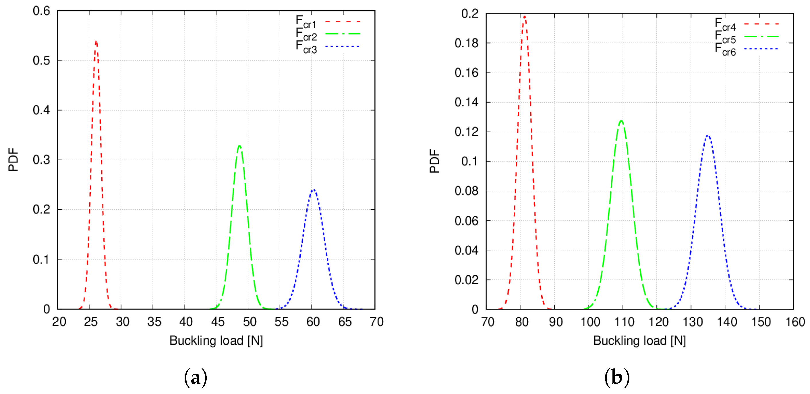
Figure 15.
(a) Case 2 , and PDFs, (b) Case 2 , and PDFs. Fibre volume fraction is treated as a Gaussian random variable with mean value and standard deviation and no fibre waviness.
Figure 15.
(a) Case 2 , and PDFs, (b) Case 2 , and PDFs. Fibre volume fraction is treated as a Gaussian random variable with mean value and standard deviation and no fibre waviness.
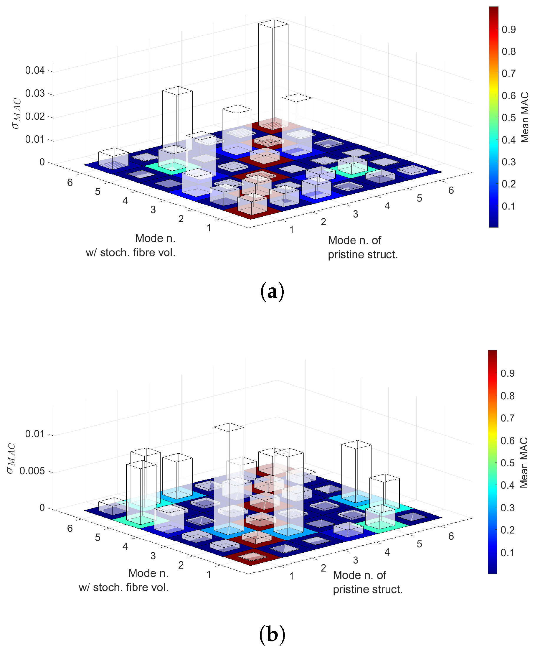
Figure 16.
(a) Case 1 3D MAC matrix, (b) Case 2 3D MAC matrix. Floor indicates the mean value and bars the standard deviation of each component of the matrix. Fibre volume fraction is treated as a Gaussian random variable with mean value and standard deviation and no fibre waviness.
Figure 16.
(a) Case 1 3D MAC matrix, (b) Case 2 3D MAC matrix. Floor indicates the mean value and bars the standard deviation of each component of the matrix. Fibre volume fraction is treated as a Gaussian random variable with mean value and standard deviation and no fibre waviness.
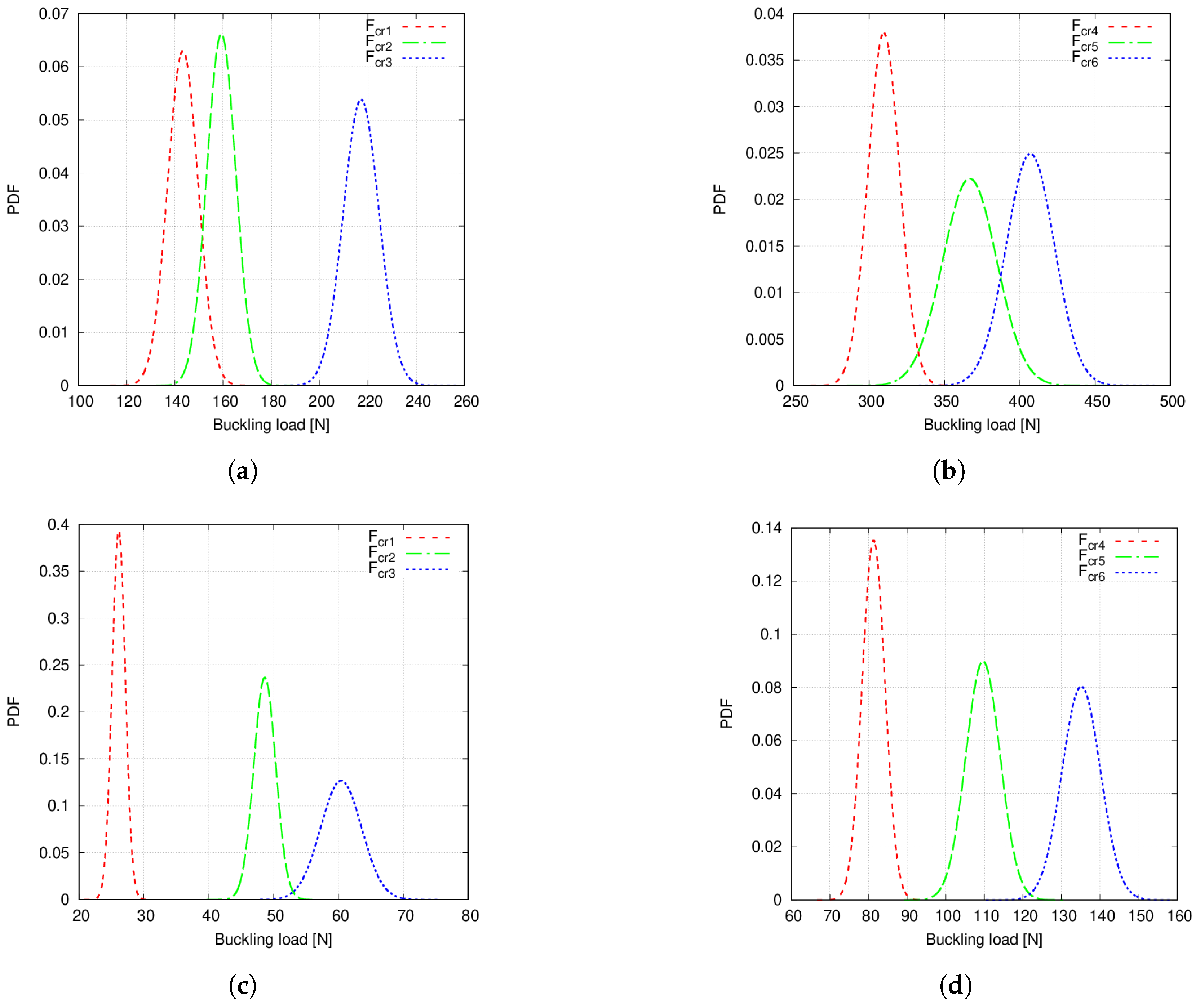
Figure 17.
(a) Case 1 , and PDFs, (b) Case 1 , and PDFs. (c) Case 2 , and PDFs. (d) Case 2 , and PDFs. Fibre volume fraction is treated as a Gaussian random variable with mean value and standard deviation whereas misalignments have a null mean and standard deviation .
Figure 17.
(a) Case 1 , and PDFs, (b) Case 1 , and PDFs. (c) Case 2 , and PDFs. (d) Case 2 , and PDFs. Fibre volume fraction is treated as a Gaussian random variable with mean value and standard deviation whereas misalignments have a null mean and standard deviation .
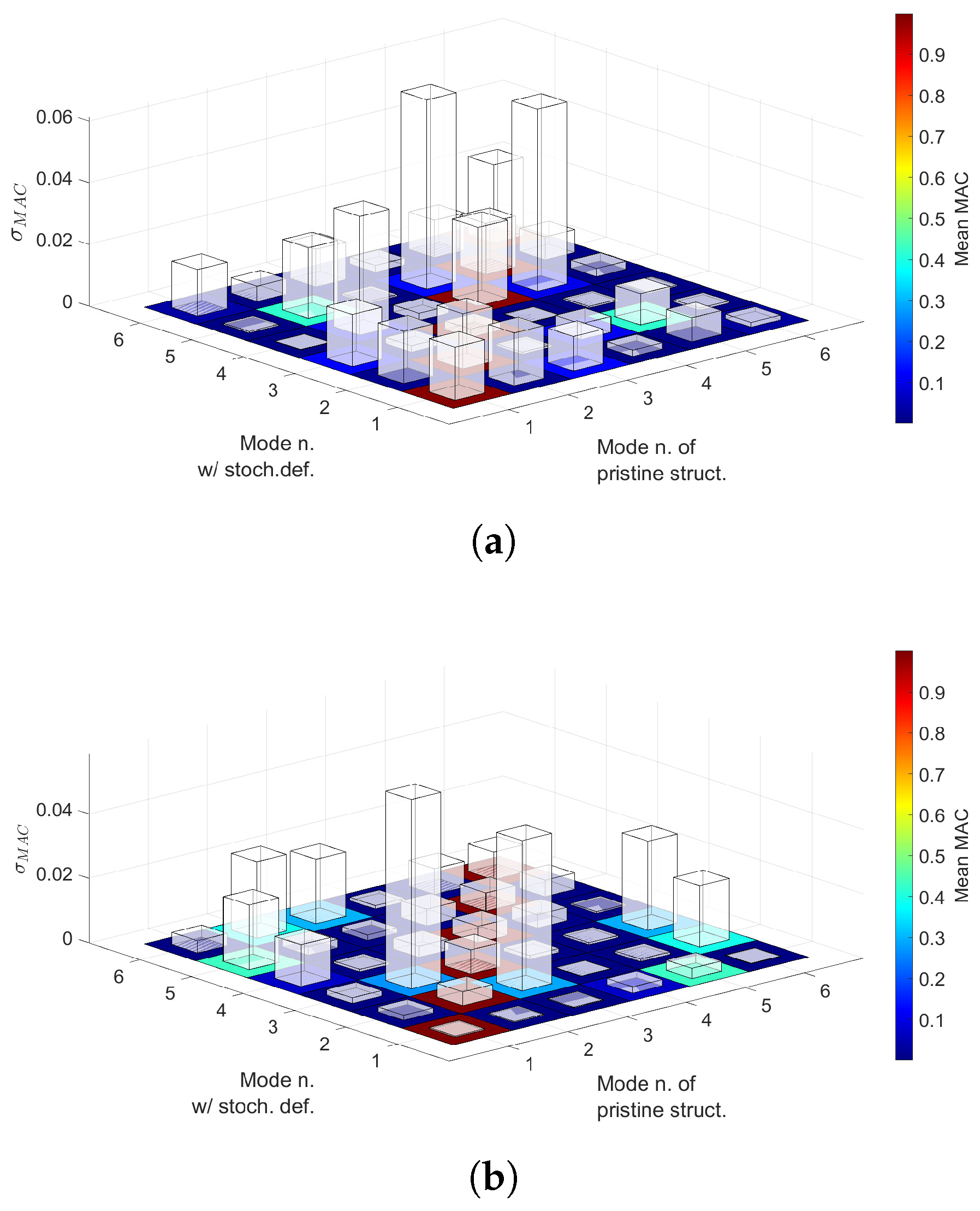
Figure 18.
(a) Case 1 3D MAC matrix, (b) Case 2 3D MAC matrix. Floor indicates the mean value and bars the standard deviation of each component of the matrix. Fibre volume fraction is treated as a Gaussian random variable with mean value and standard deviation whereas misalignments have a null mean and standard deviation .
Table 1.
Geometrical dimensions of the laminated plate.
Table 1.
Geometrical dimensions of the laminated plate.
| a [m] | b [m] | Ply Thickness [mm] |
|---|
| 0.254 | 0.254 | 0.127 |
Table 2.
Elastic properties of the constituents of the composite material and the homogenised material properties for a fibre volume fraction .
Table 2.
Elastic properties of the constituents of the composite material and the homogenised material properties for a fibre volume fraction .
| Constituent | [GPa] | [GPa] | [GPa] | [GPa] | [-] | [-] |
|---|
| Fibre | 235.0 | 14.0 | 28.0 | 5.60 | 0.20 | 0.25 |
| Matrix | 4.80 | 4.80 | 1.79 | 1.79 | 0.34 | 0.34 |
| Homogenised = 0.60 | 143.17 | 9.64 | 6.09 | 3.12 | 0.252 | 0.349 |
Table 3.
Convergence of the buckling load for the Case 1 pristine structure. A uniform fibre volume is considered and no fibre waviness.
Table 3.
Convergence of the buckling load for the Case 1 pristine structure. A uniform fibre volume is considered and no fibre waviness.
| Model | Mesh | DOF | [N] | [N] | [N] | [N] | [N] | [N] |
|---|
| Abaqus | 11 × 11 | 726 | 154.82 | 175.73 | 240.64 | 355.42 | 397.41 | 481.44 |
| | 14 × 14 | 1176 | 146.08 | 166.74 | 229.19 | 332.39 | 373.74 | 452.42 |
| | 26 × 26 | 4056 | 141.92 | 161.34 | 220.12 | 310.66 | 349.98 | 422.85 |
| | 35 × 35 | 7350 | 134.29 | 151.70 | 215.58 | 287.20 | 321.01 | 412.78 |
| | 52 × 52 | 16,224 | 133.80 | 151.11 | 214.76 | 285.49 | 318.71 | 410.53 |
| Cubic | 2B4-2L16 | 2184 | 163.98 | 186.71 | 255.72 | 391.69 | 440.89 | 521.07 |
| | 4B4-4L16 | 7098 | 143.59 | 159.08 | 216.77 | 310.22 | 366.45 | 407.53 |
| | 6B4-6L16 | 14,820 | 142.01 | 156.24 | 211.10 | 294.06 | 349.56 | 390.31 |
| | 8B4-8L16 | 25,350 | 141.64 | 155.57 | 209.82 | 290.89 | 345.89 | 386.11 |
| Quadratic | 4B3-4L9 | 2430 | 209.87 | 236.55 | 311.29 | 436.55 | 501.59 | 570.80 |
| | 6B3-6L9 | 4914 | 168.20 | 187.70 | 251.96 | 367.75 | 414.15 | 477.14 |
| | 8B3-8L9 | 8262 | 155.93 | 172.94 | 232.71 | 333.21 | 384.60 | 436.97 |
| | 10B3-10L9 | 12,474 | 150.49 | 166.32 | 223.96 | 316.89 | 370.03 | 417.18 |
| | 12B3-12L9 | 17,550 | 145.85 | 160.64 | 216.41 | 302.76 | 356.92 | 400.51 |
Table 4.
Convergence of the buckling load for the Case 2 pristine structure. A uniform fibre volume is considered and no fibre waviness.
Table 4.
Convergence of the buckling load for the Case 2 pristine structure. A uniform fibre volume is considered and no fibre waviness.
| Model | Mesh | DOF | [N] | [N] | [N] | [N] | [N] | [N] |
|---|
| Abaqus | 11 × 11 | 726 | 26.49 | 51.56 | 64.29 | 88.30 | 137.57 | 168.73 |
| | 14 × 14 | 1176 | 25.75 | 49.55 | 61.27 | 83.54 | 121.31 | 149.29 |
| | 26 × 26 | 4056 | 24.99 | 47.35 | 58.64 | 78.90 | 107.40 | 132.03 |
| | 35 × 35 | 7350 | 24.71 | 47.02 | 57.67 | 78.09 | 104.31 | 129.26 |
| | 52 × 52 | 16,224 | 24.67 | 46.75 | 57.55 | 77.59 | 103.26 | 127.54 |
| Cubic | 2B4-2L16 | 2184 | 27.90 | 59.06 | 91.21 | 141.54 | 322.77 | 387.92 |
| | 4B4-4L16 | 7098 | 26.05 | 48.64 | 60.27 | 81.31 | 109.39 | 134.89 |
| | 6B4-6L16 | 14,820 | 25.42 | 46.97 | 58.29 | 77.04 | 108.59 | 128.68 |
| | 8B4-8L16 | 25,350 | 25.21 | 46.49 | 57.75 | 76.33 | 105.89 | 124.91 |
| Quadratic | 4B3-4L9 | 2430 | 34.83 | 69.15 | 89.79 | 137.56 | 323.65 | 391.87 |
| | 6B3-6L9 | 4914 | 29.65 | 56.91 | 72.49 | 101.51 | 154.18 | 196.38 |
| | 8B3-8L9 | 8262 | 27.77 | 52.52 | 65.55 | 89.78 | 134.59 | 163.93 |
| | 10B3-10L9 | 12,474 | 26.84 | 50.33 | 62.49 | 84.59 | 123.75 | 148.71 |
| | 12B3-12L9 | 17,550 | 26.33 | 49.13 | 60.92 | 81.87 | 117.82 | 140.63 |
Table 5.
Dimensionless CPU time for the different meshes employed with the present LW approach.
Table 5.
Dimensionless CPU time for the different meshes employed with the present LW approach.
| Model | Mesh | DOF | [-] |
|---|
| Cubic | 2B4-2L16 | 2184 | 0.30 |
| | 4B4-4L16 | 7098 | 1.00 |
| | 6B4-6L16 | 14,820 | 2.47 |
| | 8B4-8L16 | 25,350 | 4.23 |
| Quadratic | 4B3-4L9 | 2430 | 0.01 |
| | 6B3-6L9 | 4914 | 0.22 |
| | 8B3-8L9 | 8262 | 0.37 |
| | 10B3-10L9 | 12,474 | 0.55 |
| | 12B3-12L9 | 17,550 | 0.79 |
Table 6.
Case 1 critical buckling loads mean value and standard deviation calculated by means of pure Monte Carlo and first- and second-order PCE.
Table 6.
Case 1 critical buckling loads mean value and standard deviation calculated by means of pure Monte Carlo and first- and second-order PCE.
| Buckling | Deterministic | Monte Carlo | 1st Order PCE | 2nd Order PCE | Monte Carlo | 1st Order PCE | 2nd Order PCE |
|---|
| Load | Value [N] | Mean [N] | Mean [N] | Mean [N] | COV [%] | COV [%] | COV [%] |
|---|
| 143.59 | 143.48 | 143.48 | 143.49 | 3.14 | 3.16 | 3.16 |
| 159.07 | 159.21 | 159.21 | 159.21 | 3.07 | 3.08 | 3.09 |
| 216.77 | 217.16 | 217.16 | 217.16 | 3.20 | 3.22 | 3.21 |
| 310.21 | 310.47 | 310.46 | 310.48 | 3.11 | 3.12 | 3.12 |
| 366.45 | 366.61 | 366.61 | 366.62 | 3.27 | 3.31 | 3.31 |
| 407.53 | 407.91 | 407.91 | 407.93 | 3.24 | 3.11 | 3.10 |
Table 7.
Case 2 critical buckling loads mean value and standard deviation calculated by means of pure Monte Carlo and first- and second-order PCE.
Table 7.
Case 2 critical buckling loads mean value and standard deviation calculated by means of pure Monte Carlo and first- and second-order PCE.
| Buckling | Deterministic | Monte Carlo | 1st Order PCE | 2nd Order PCE | Monte Carlo | 1st Order PCE | 2nd Order PCE |
|---|
| Load | Value [N] | Mean [N] | Mean [N] | Mean [N] | COV [%] | COV [%] | COV [%] |
|---|
| 26.05 | 26.10 | 26.10 | 26.10 | 2.81 | 2.84 | 2.84 |
| 48.64 | 48.66 | 48.66 | 48.66 | 2.49 | 2.49 | 2.50 |
| 60.27 | 60.30 | 60.29 | 60.30 | 2.75 | 2.76 | 2.75 |
| 81.31 | 81.29 | 81.29 | 81.29 | 2.48 | 2.48 | 2.48 |
| 109.3 | 109.58 | 109.58 | 109.58 | 2.85 | 2.86 | 2.86 |
| 134.89 | 134.96 | 134.96 | 134.96 | 2.52 | 2.51 | 2.51 |
Table 8.
Computational time needed to: perform a Monte Carlo analysis consisting of samples; obtain 300 samples to construct the PCE surrogate, and emulate samples using PCE.
Table 8.
Computational time needed to: perform a Monte Carlo analysis consisting of samples; obtain 300 samples to construct the PCE surrogate, and emulate samples using PCE.
| Monte Carlo [hours] | PCE Build-Up [hours] | PCE Usage [s] |
|---|
| 71 | 21 | 3 |
Table 9.
Correlation indices between Case 1 buckling loads.
Table 9.
Correlation indices between Case 1 buckling loads.
| | |
|---|
| 0.998 | 0.912 | 0.988 |
Table 10.
Case 1 critical buckling loads mean value and COV calculated by means of first- and second-order PCE considering spatially varying fibre volume fraction and fibre misalignments.
Table 10.
Case 1 critical buckling loads mean value and COV calculated by means of first- and second-order PCE considering spatially varying fibre volume fraction and fibre misalignments.
| Buckling | Deterministic | 1st Order PCE | 2nd Order PCE | 1st Order PCE | 2nd Order PCE |
|---|
| Load | Load [N] | Mean [N] | Mean [N] | COV [%] | COV [%] |
|---|
| 143.59 | 143.30 | 143.34 | 4.52 | 4.42 |
| 159.07 | 159.29 | 159.26 | 3.91 | 3.79 |
| 216.77 | 217.22 | 217.23 | 3.61 | 3.41 |
| 310.21 | 309.82 | 309.76 | 3.59 | 3.39 |
| 366.45 | 366.75 | 366.76 | 5.02 | 4.88 |
| 407.53 | 407.09 | 406.99 | 4.05 | 3.93 |
Table 11.
Case 2 critical buckling loads mean value and COV calculated by means of first- and second-order PCE considering spatially varying fibre volume fraction and fibre misalignments.
Table 11.
Case 2 critical buckling loads mean value and COV calculated by means of first- and second-order PCE considering spatially varying fibre volume fraction and fibre misalignments.
| Buckling | Deterministic | 1st Order PCE | 2nd Order PCE | 1st Order PCE | 2nd Order PCE |
|---|
| Load | Load [N] | Mean [N] | Mean [N] | COV [%] | COV [%] |
|---|
| 26.05 | 26.13 | 26.14 | 3.96 | 3.88 |
| 48.64 | 48.65 | 48.65 | 3.57 | 3.46 |
| 60.27 | 60.42 | 60.41 | 5.32 | 5.22 |
| 81.31 | 81.32 | 81.32 | 3.72 | 3.63 |
| 109.30 | 109.67 | 109.66 | 4.08 | 4.05 |
| 134.89 | 135.11 | 135.11 | 3.75 | 3.68 |


