
Revisiting the Characterization of the Losses in Piezoelectric Materials from Impedance Spectroscopy at Resonance

Abstract
:
1. Introduction
1.1. Losses in Piezoelectric Materials
1.2. Imaginary Part versus Phase Angle

1.3. Dielectric and Mechanical Losses
1.4. The Matrix of Coefficients
1.5. Piezoelectric Losses
2. Material Characterization from Electromechanical Resonances
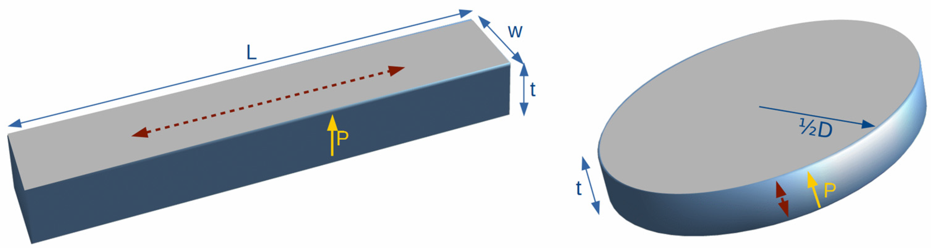
2.1. Shapes and Modes
2.2. The Iterative Method

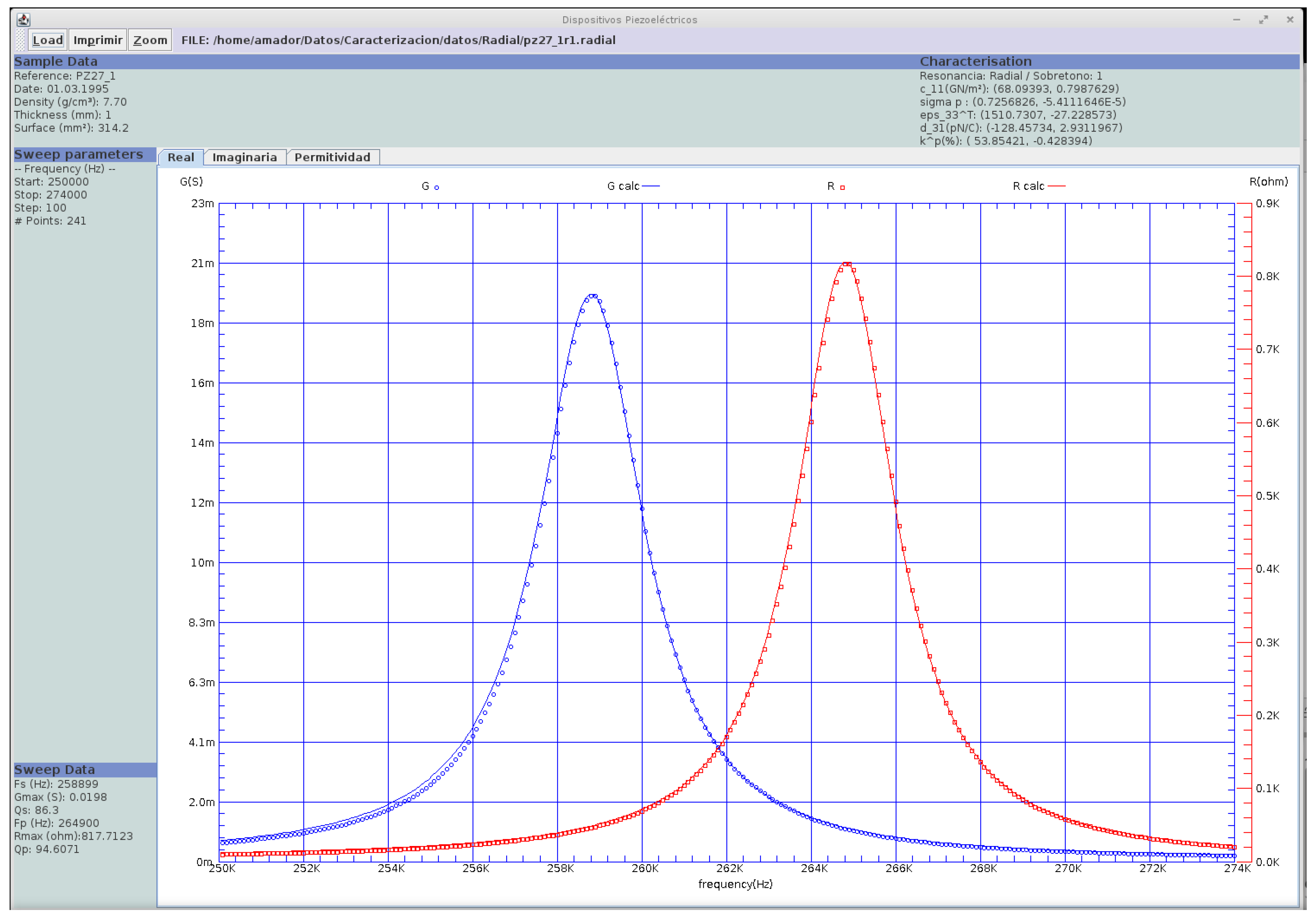
2.3. Plotting Data


3. Studying Losses
3.1. What Losses Look Like?

| Shape | Rod |
|---|---|
| mode | length extensional |
| Thickness (m) | 0.65 × 10⁻³ |
| length (m) | 31.3 × 10⁻³ |
| width (m) | 1.46 × 10⁻³ |
| density () | |
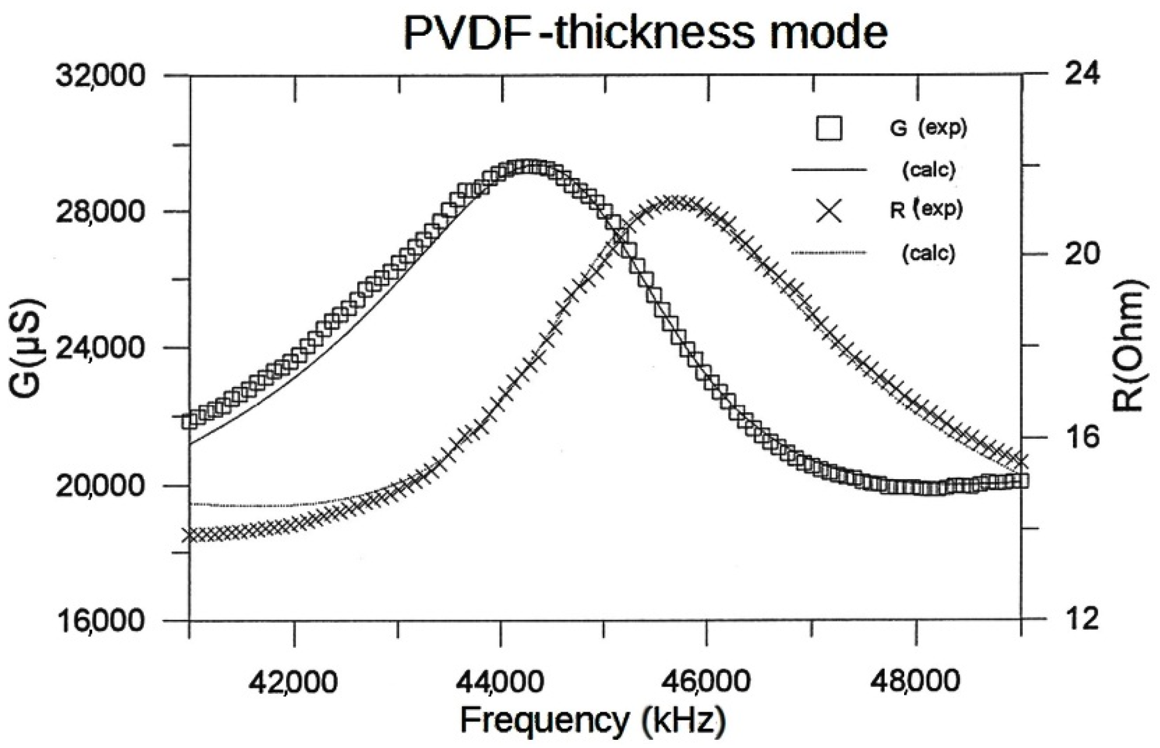
| Shape | Disc |
| mode | thickness extensional |
| Thickness (m) | 1.00 × 10⁻³ |
| radius (m) | 20.0 × 10⁻³ |
| density | |

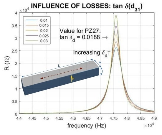
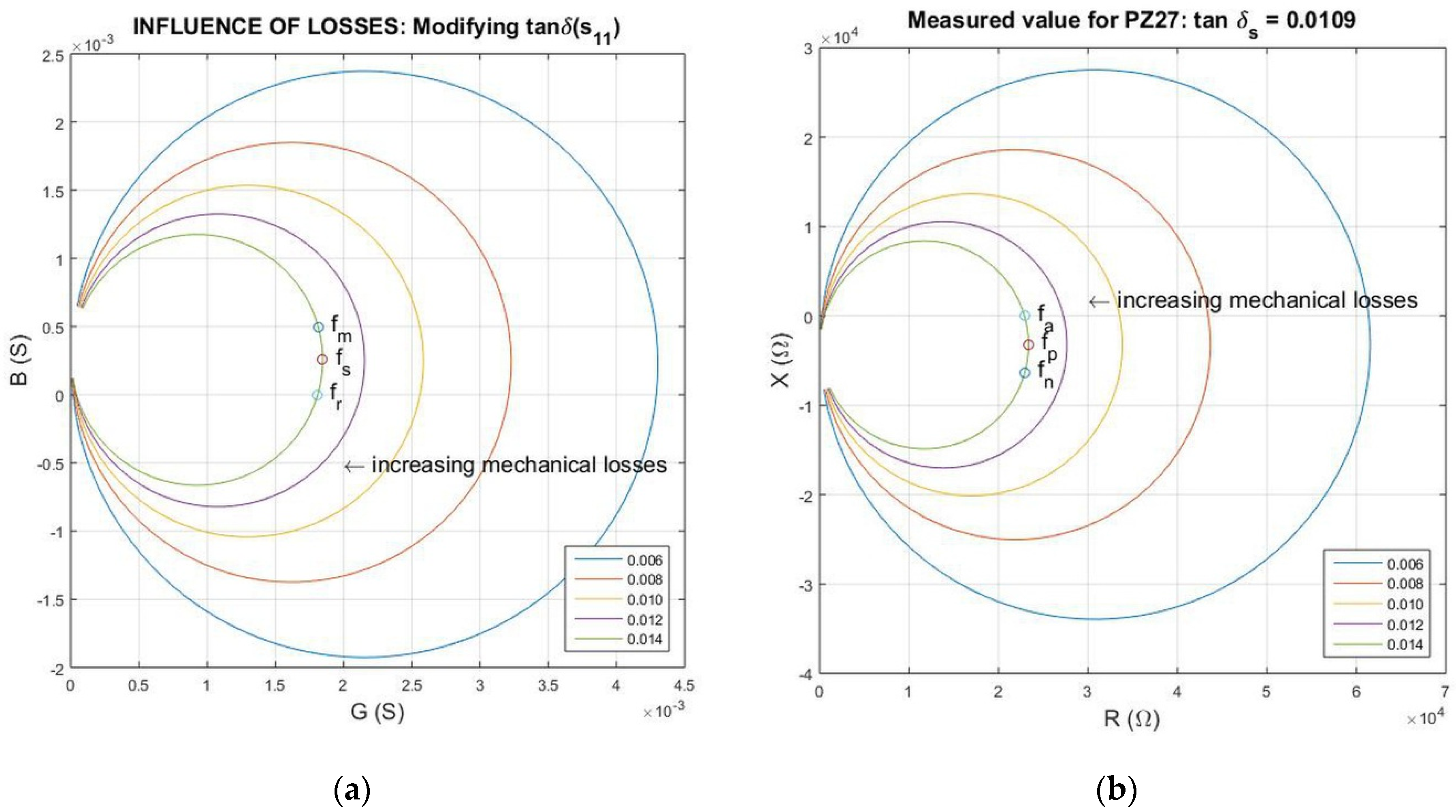
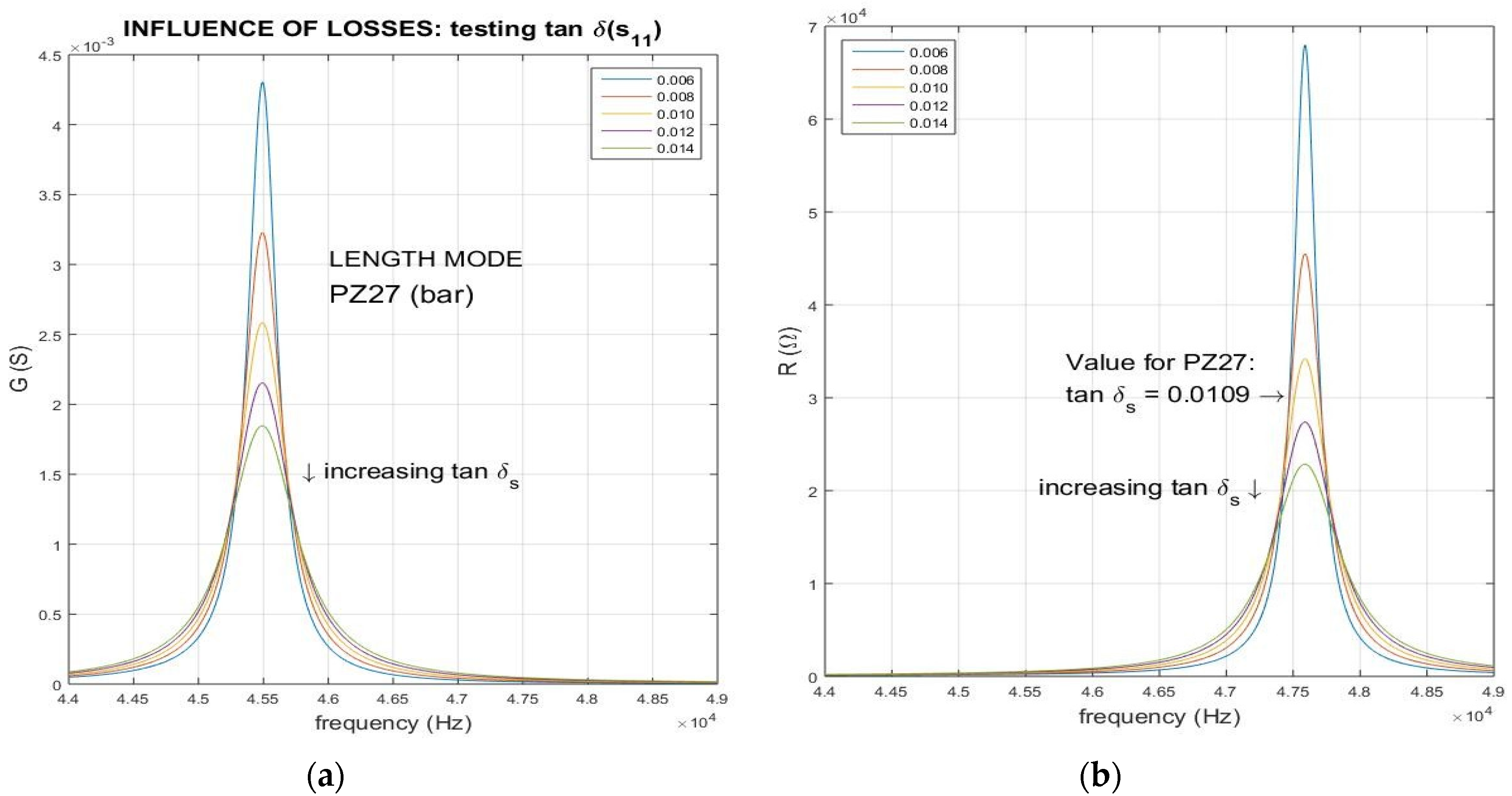
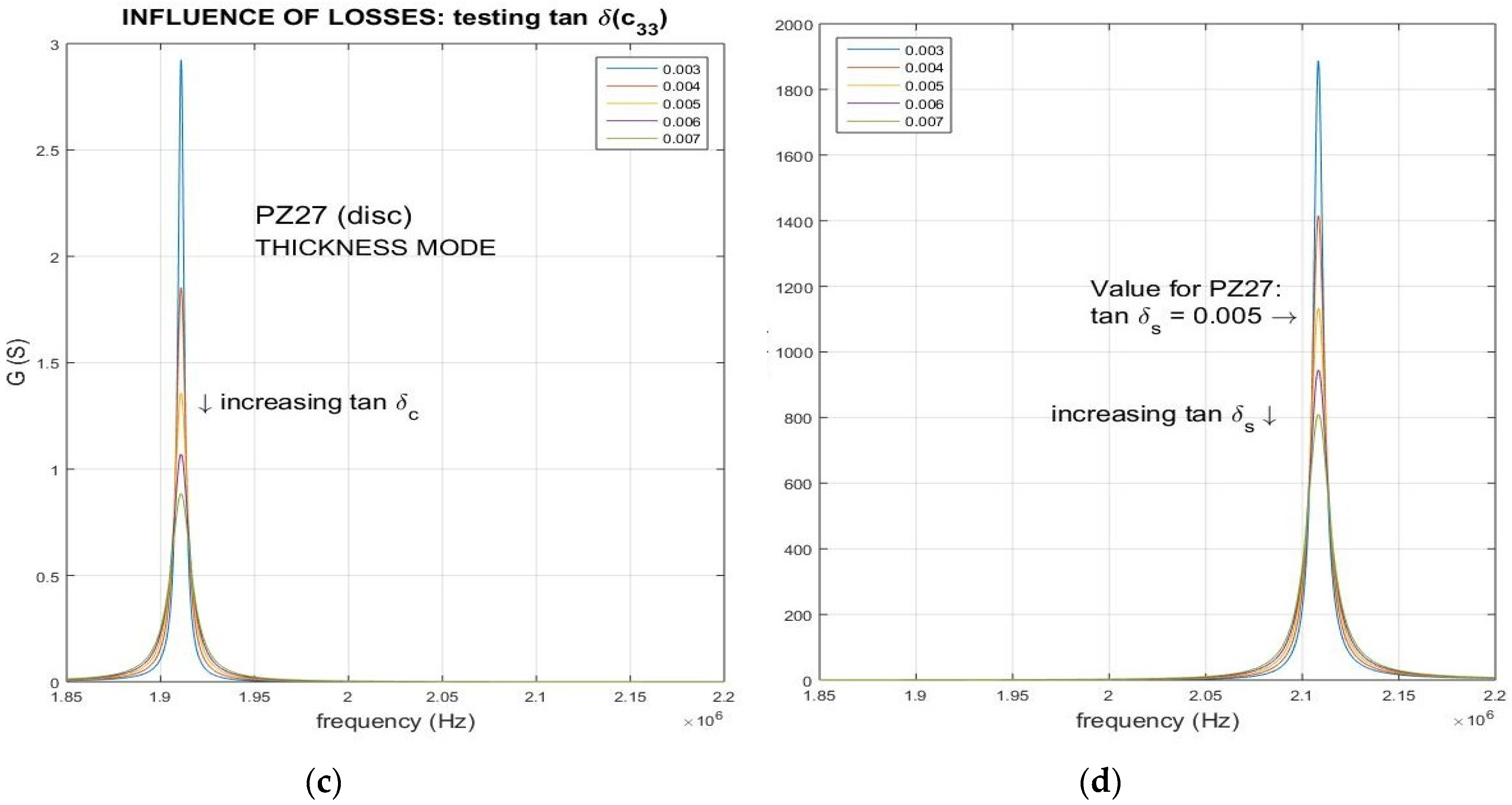
3.2. Influence of the Mechanical Losses


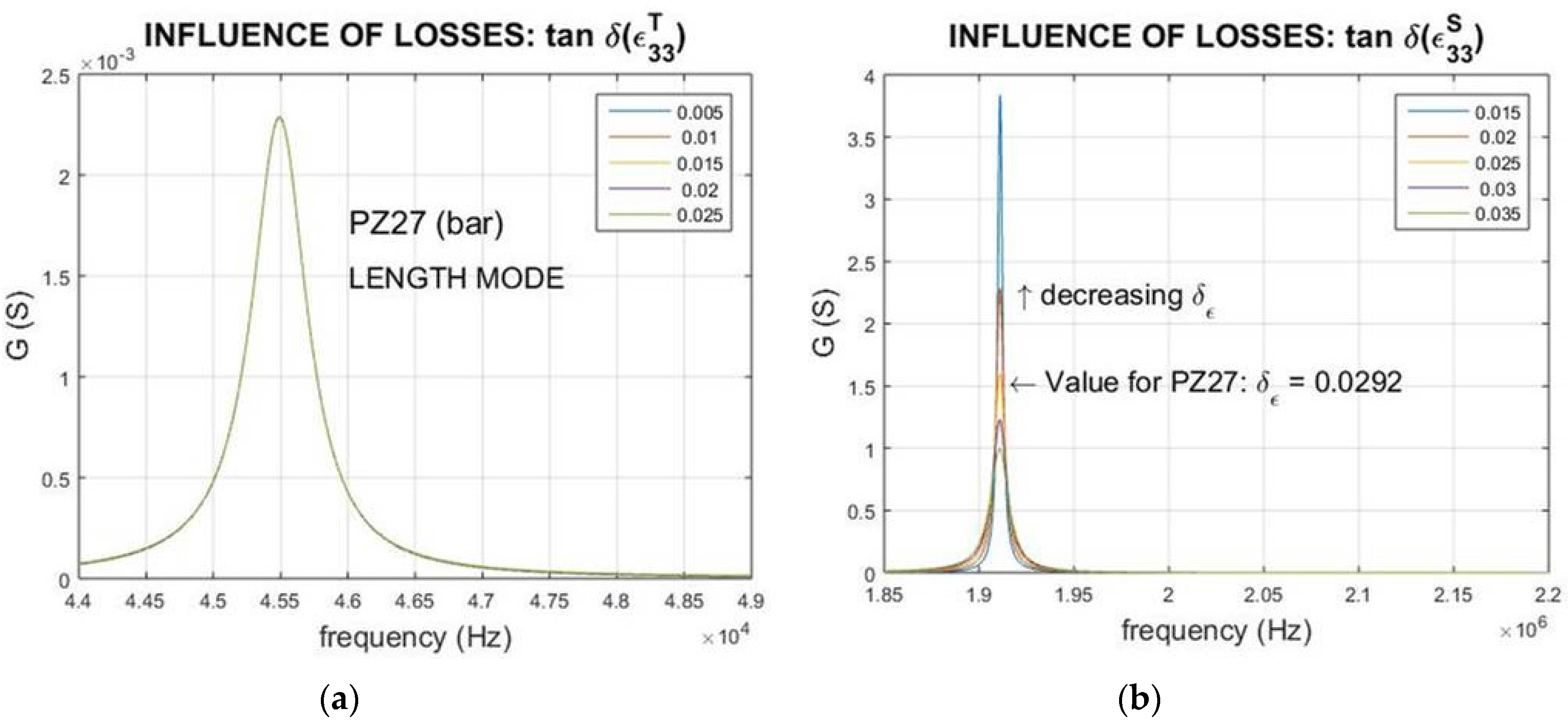
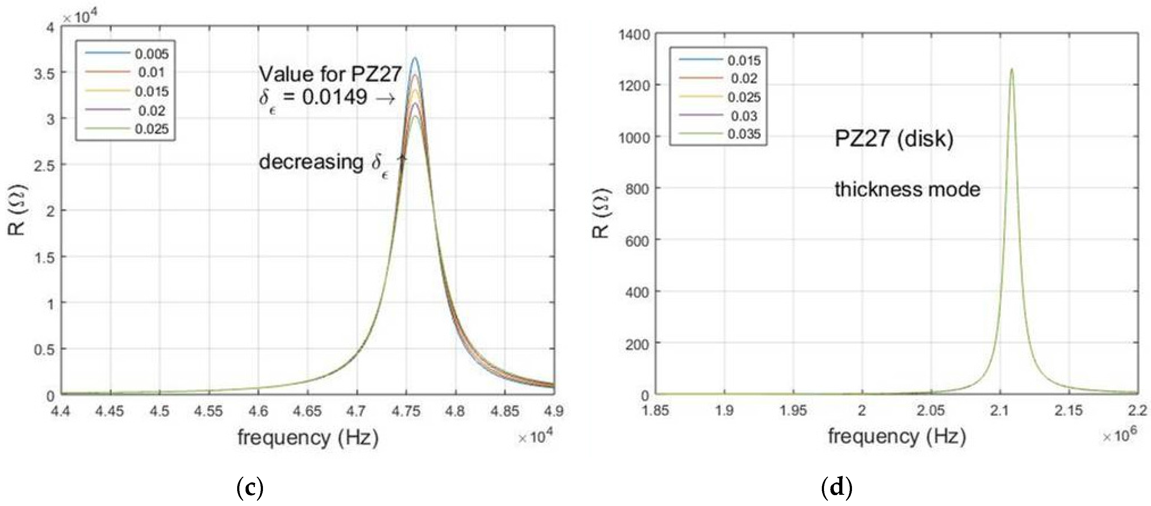
3.3. Influence of the Dielectric Losses


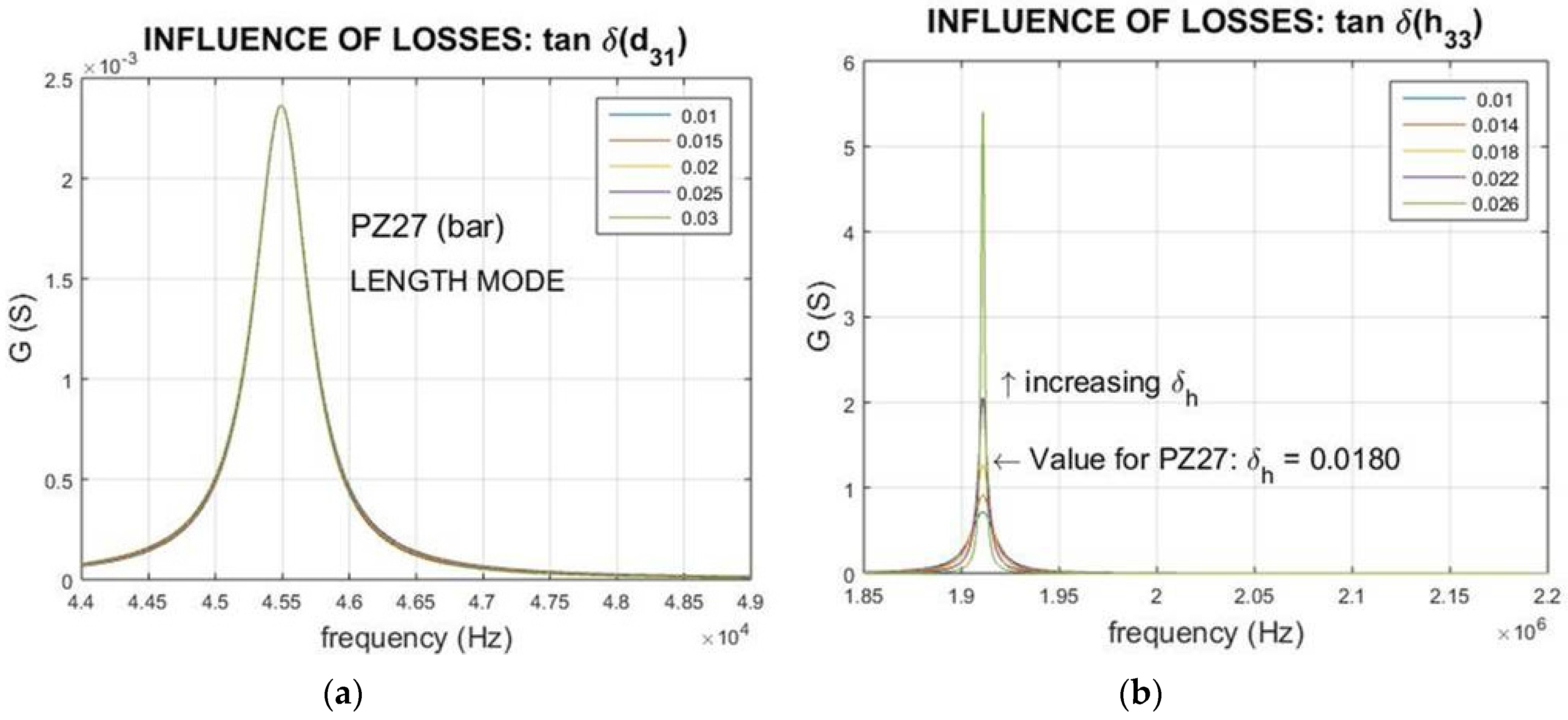
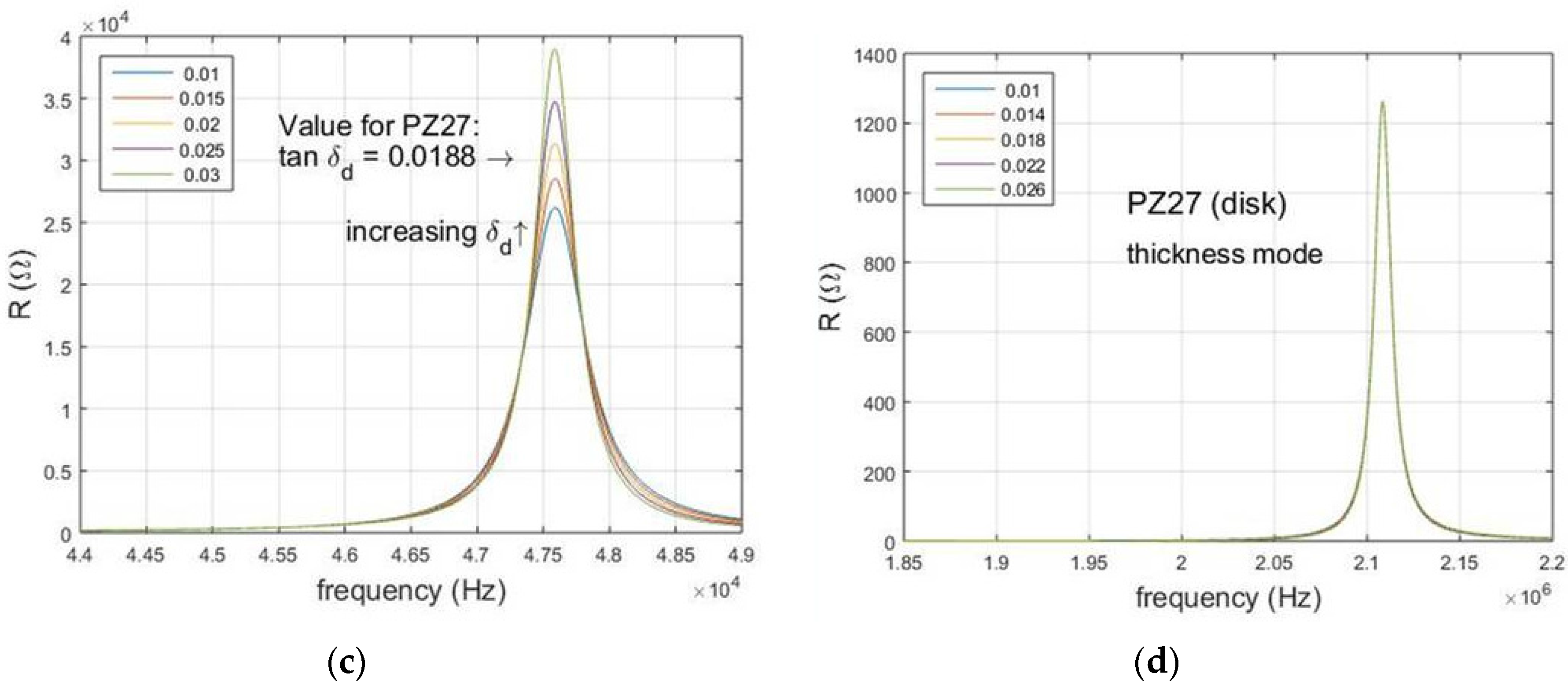
3.4. Influence of the Piezoelectric Losses (Piezoelectric Modulus)


4. Losses in Devices


5. Conclusions
Acknowledgments
Author Contributions
Conflicts of Interest
References
- Cady, W.G. Piezoelectricity: An Introduction to the Theory and Applications of Electromechanical Phenomena in Crystals; Mc Graw Hill Book Co.: New York, NY, USA, 1946. [Google Scholar]
- Jaffe, B.; Cook, W.R.; Jaffe, H. Piezoelectric Ceramics; Academic Press: New York, NY, USA, 1971. [Google Scholar]
- Fukada, E. History and recent progress in piezoelectric polymers. IEEE Trans. Ultrason. Ferroelectr. Freq. Control 2000, 47, 1277–1290. [Google Scholar] [CrossRef] [PubMed]
- Newnham, R.E.; Skinner, D.P.; Cross, L.E. Connectivity and piezoelectric-pyroelectric composites. Mat. Res. Bull. 1978, 13, 525–536. [Google Scholar] [CrossRef]
- Holland, R. Representation of dielectric, elastic, and piezoelectric losses by complex coefficients. IEEE Trans. Sonics Ultrason. 1967, 14, 18–20. [Google Scholar] [CrossRef]
- Martin, G.E. Dielectric, Elastic and Piezoelectric Losses in Piezoelectric Materials. In Proceedings of the 1974 Ultrasonics Symposium, University of Wisconsin-Milwakee, Milwaukee, WI, USA, 11–14 November 1974; pp. 613–617.
- Arlt, G.; Dederichs, H. Complex elastic, dielectric and piezoelectric constants by domain wall damping in ferroelectric ceramics. Ferroelectrics 1980, 29, 47–50. [Google Scholar] [CrossRef]
- Damjanovic, D.; Gururaja, T.R.; Jang, S.J.; Cross, L.E. Temperature behavior of the complex piezoelectric d31, coefficient in modified lead titanate ceramics. Mater. Lett. 1986, 4, 414. [Google Scholar] [CrossRef]
- Sherrit, S; Mukherjee, B.K. The use of complex material constants to model the dynamic response of piezoelectric materials. In Proceedings of the Ultrasonics Symposium, Sendai, Japan, 5–8 October 1998; Volume 1, pp. 633–640.
- Uchino, K.; Zhuang, Y.; Ural, S.O. Loss determination methodology for a piezoelectric ceramic: New phenomenological theory and experimental proposals. J. Adv. Dielectr. 2011, 1, 17–31. [Google Scholar] [CrossRef]
- Mezheritsky, A.V. Efficiency of excitation of piezoceramic transducers at antiresonance frequency. IEEE Trans. Ultrason. Ferroelectr. Freq. Control 2002, 49, 484–494. [Google Scholar] [CrossRef] [PubMed]
- Lu, X.; Hanagud, S.V. Extended Irreversible Thermodynamics Modeling for Self-Heating and Dissipation in Piezoelectric Ceramics. IEEE Trans. Ultrason. Ferroelectr. Freq. Control 2004, 51, 1582–1592. [Google Scholar] [PubMed]
- Hagiwara, M.; Hoshina, T.; Takeda, H.; Tsurumi, T. Identicalness between Piezoelectric Loss and Dielectric Loss in Converse Effect of Piezoelectric Ceramic Resonators. Jpn. J. Appl. Phys. 2012, 51, 09LD10. [Google Scholar] [CrossRef]
- Cain, M.G.; Stewart, M. Losses in Piezoelectrics via Complex Resonance Analysis. In Characterisation of Ferroelectric Bulk Materials and Thin Films; Cain, M.G., Ed.; Springer Series in Measurement Science and Technology: New York, NY, USA, 2014; Volume 2. [Google Scholar]
- Liu, G.; Zhang, S.; Jiang, W.; Cao, W. Losses in ferroelectric materials. Mater. Sci. Eng. R Rep. 2015, 89, 1–48. [Google Scholar] [CrossRef] [PubMed]
- IEEE Standard on Piezoelectricity; ANSI/IEEE Std. 176–1987; IEEE Society: Washinton D.C., WA, USA, 1987.
- Nye, J.F. Physical Properties of Crystals; Oxford University Press Inc.: New York, NY, USA, 1957. [Google Scholar]
- Vicente, J.M.; Jimenez, B. Frequency dependence of the piezoelectric d31 coefficient as a function of ceramic tetragonality. Ferroelectrics 1992, 134, 157–162. [Google Scholar] [CrossRef]
- Jimenez, B.; Vicente, J.M. Influence of mobile 90° domains on the complex elastic modulus of PZT ceramics. J. Phys. D: Appl. Phys. 2000, 33, 1525–1535. [Google Scholar] [CrossRef]
- Alemany, C.; Pardo, L.; Jimenez, B.; Carmona, F.; Mendiola, J.; Gonzalez, A. Automatic iterative evaluation of complex material constants in piezoelectric ceramics. J. Phys. D Appl. Phys. 1994, 27, 148. [Google Scholar]
- Piezoelectric Resonance Analysis Program. Available online: http://www.tasitechnical.com/products.html (accessed on 30 October 2015).
- Pardo, L. Piezoelectric materials for power ultrasonic transducers. In Power Ultrasonics; Gallego-Juárez, J.A., Graff, K., Eds.; Woodhead Publishing Ltd.: Cambridge, UK, 2014. [Google Scholar]
- Rupitsch, S.J. Complete Characterization of Piezoceramic Materials by Means of Two Block-Shaped Test Samples. IEEE Trans. Ultrason. Ferroelectr. Freq. Control 2015, 62, 1403–1413. [Google Scholar] [CrossRef] [PubMed]
- Kiyono, C.Y.; Peréz, N.; Silva, E.C.N. Determination of full piezoelectric complex parameters using gradient-based optimization algorithm. Smart Mater. Structs 2016. [Google Scholar] [CrossRef]
- Alemany, C.; Gonzalez, A.; Pardo, L.; Jimenez, B.; Carmona, F.; Mendiola, J. Automatic determination of complex constants of piezoelectric lossy materials in the radial mode. J. Phys. D Appl. Phys. 1995, 28, 945–956. [Google Scholar] [CrossRef]
- Experimental Techniques (ICMM-CSIC). Available online: http://icmm.csic.es/gf2/medidas.htm (accessed on 30 October 2015).
- Smits, J.G. Iterative method for accurate determination of the real and imaginary parts of the materials coefficients of piezoelectric ceramics. IEEE Trans. Sonics Ultrason. 1976, 23, 393–402. [Google Scholar] [CrossRef]
- Algueró, M.; Alemany, C.; Pardo, L.; Gonzalez, A.M. Method for obtaining the full set of linear electric, mechanical and electromechanical coefficients and all related losses of a piezoelectric ceramic. J. Am. Ceram. Soc. 2004, 87, 209–215. [Google Scholar] [CrossRef]
- Gonzalez, A.M.; Alemany, C. Determination of the frequency dependence of characteristic constants in lossy piezoelectric materials. J. Phys. D: Appl. Phys. 1996, 29, 2476–2482. [Google Scholar] [CrossRef]
- Gonzalez, A.M.; Alemany, C. Estudio de los sobretonos del modo de vibración en espesor de resonadores piezoeléctricos con pérdidas. Bol. Soc. Esp. Ceram. Vid. 1995, 34, 368–371. [Google Scholar]
- Pardo, L.; Jiménez, R.; García, A.; Brebøl, K.; Leighton, G.; Huang, Z. Impedance measurements for determination of the elastic and piezoelectric coefficients of films. Adv. Appl. Ceram.: Struct. Funct. Bioceram. 2010, 109, 156–161. [Google Scholar] [CrossRef]
- Pardo, L.; García, A.; de Espinosa, F.M.; Brebøl, K. Shear Resonance Mode Decoupling to Determine the Characteristic Matrix of Piezoceramics For 3-D Modelling. IEEE Trans. Ultrason. Ferroelectr. Freq. Control 2011, 58, 646–657. [Google Scholar] [CrossRef] [PubMed]
- Guennou, M.; Dammak, H.; Djémi, P.; Moch, P.; Pham-Thi, M. Electromechanical properties of single domain PZN–12%PT measured by three different methods. Solid State Sci. 2010, 12, 298–301. [Google Scholar] [CrossRef]
- Sherrit, S.; Masys, T.J.; Wiederick, H.D.; Mukherjee, B.K. Determination of the reduced matrix of the piezoelectric, dielectric, and elastic material constants for a piezoelectric material with C∞ symmetry. IEEE Trans. Ultrason. Ferroelectr. Freq. Control 2011, 58, 1714–1720. [Google Scholar] [CrossRef] [PubMed]
- Gonzalez, A.M.; de Frutos, J.; Duro, M.C. Procedure for the Characterization of Piezoelectric Samples in Non-standard Resonant Modes. J. Eur. Ceram. Soc. 1999, 19, 1285–1288. [Google Scholar] [CrossRef]
- Martin, G.E. Determination of Equivalent-Circuit Constants of Piezoelectric Resonators of Moderately Low Q by Absolute-Admittance Measurements. J. Acoust. Soc. Am. 1954, 26, 413–420. [Google Scholar] [CrossRef]
- Tilmans, H.A.C. Equivalent circuit representation of electromechanical transducers: I. Lumped -parameter systems. J. Micromech. Microeng. 1996, 6, 157–176. [Google Scholar] [CrossRef]
- Tilmans, H.A.C. Equivalent circuit representation of electromechanical transducers: II. Distributed-parameter systems. J. Micromech. Microeng. 1997, 7, 285–309. [Google Scholar] [CrossRef]
- Sherrit, S.; Leary, S.P.; Dolgin, B.P.; Bar-Cohen, Y. Comparison of the Mason and KLM equivalent circuits for piezoelectric resonators in the thickness mode. In Proceedings of the Ultrasonics Symposium, Caesars Tahoe, NV, USA, 17–20 October 1999; pp. 921–926.
- Guisado, A.; Torres, J.L.; González, A.M. Study of Equivalent Circuits of Piezoceramics to Use in Simulations with Pspice. Ferroelectrics 2003, 293, 307–319. [Google Scholar] [CrossRef]
- Ballato, A. Modeling piezoelectric and piezomagnetic devices and structures via equivalent networks. IEEE Trans. Ultrason. Ferroelectr. Freq. Control 2001, 48, 405–414. [Google Scholar] [CrossRef]
- Püttmer, A.; Hauptmann, P.; Lucklum, R.; Krause, O.; Henning, B. SPICE Model for Lossy Piezoceramic Transducers. IEEE Trans. Ultrason. Ferroelectr. Freq. Control 1997, 44, 60–66. [Google Scholar] [CrossRef] [PubMed]
- Alcocer, E.M. Modelado y Simulación de Sensores y Actuadores Para Ultrasonidos. Bachelor’s Thesis, Tecnical University of Madrid-EUIT Telecomunicación, Madrid, Spain, 2003. Available online: http://marte.biblioteca.upm.es/ (accessed on 21 January 2016). [Google Scholar]
© 2016 by the authors; licensee MDPI, Basel, Switzerland. This article is an open access article distributed under the terms and conditions of the Creative Commons by Attribution (CC-BY) license (http://creativecommons.org/licenses/by/4.0/).
Share and Cite
González, A.M.; García, Á.; Benavente-Peces, C.; Pardo, L. Revisiting the Characterization of the Losses in Piezoelectric Materials from Impedance Spectroscopy at Resonance. Materials 2016, 9, 72. https://doi.org/10.3390/ma9020072
González AM, García Á, Benavente-Peces C, Pardo L. Revisiting the Characterization of the Losses in Piezoelectric Materials from Impedance Spectroscopy at Resonance. Materials. 2016; 9(2):72. https://doi.org/10.3390/ma9020072
Chicago/Turabian StyleGonzález, Amador M., Álvaro García, César Benavente-Peces, and Lorena Pardo. 2016. "Revisiting the Characterization of the Losses in Piezoelectric Materials from Impedance Spectroscopy at Resonance" Materials 9, no. 2: 72. https://doi.org/10.3390/ma9020072