A Review of Feature Extraction Methods in Vibration-Based Condition Monitoring and Its Application for Degradation Trend Estimation of Low-Speed Slew Bearing


Abstract
:1. Introduction
2. Laboratory Slew Bearing Experiment
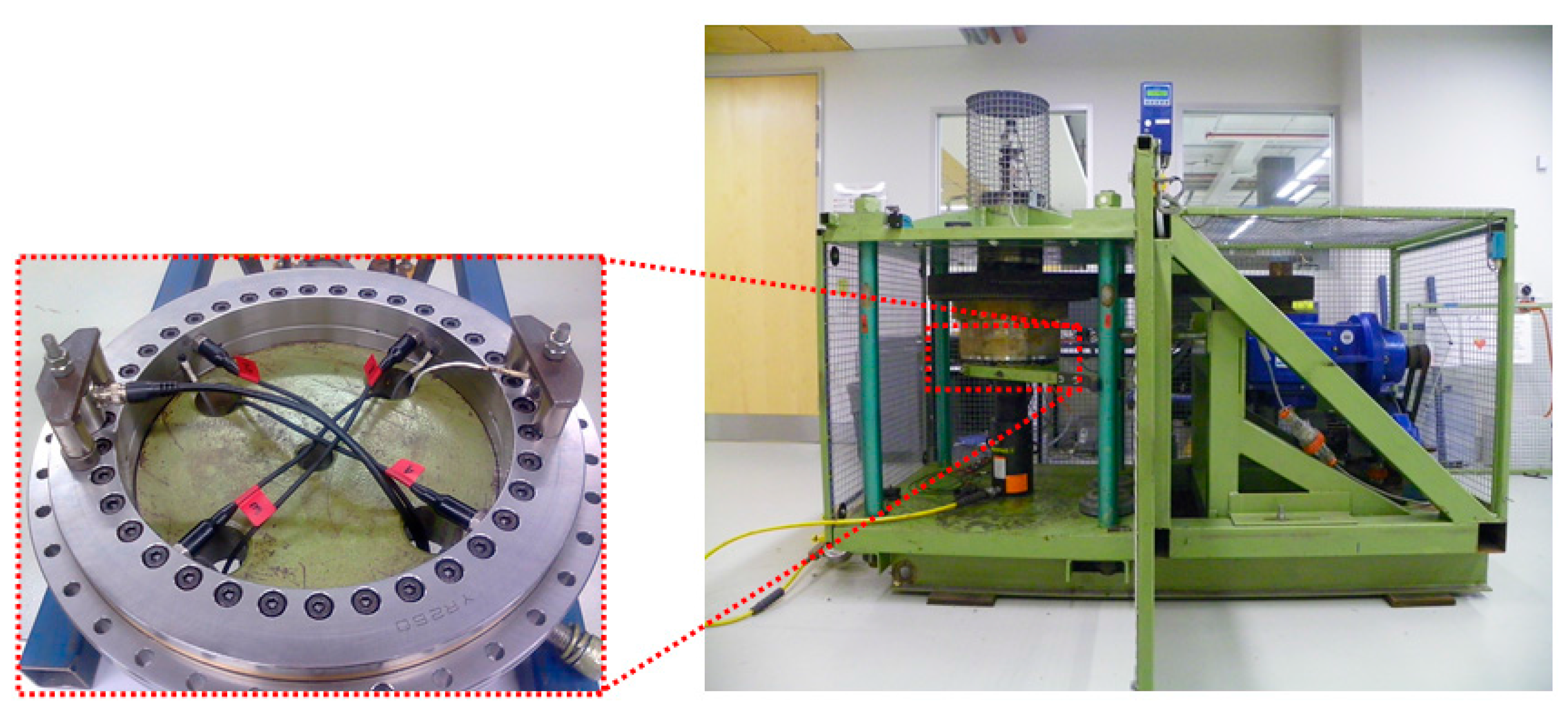
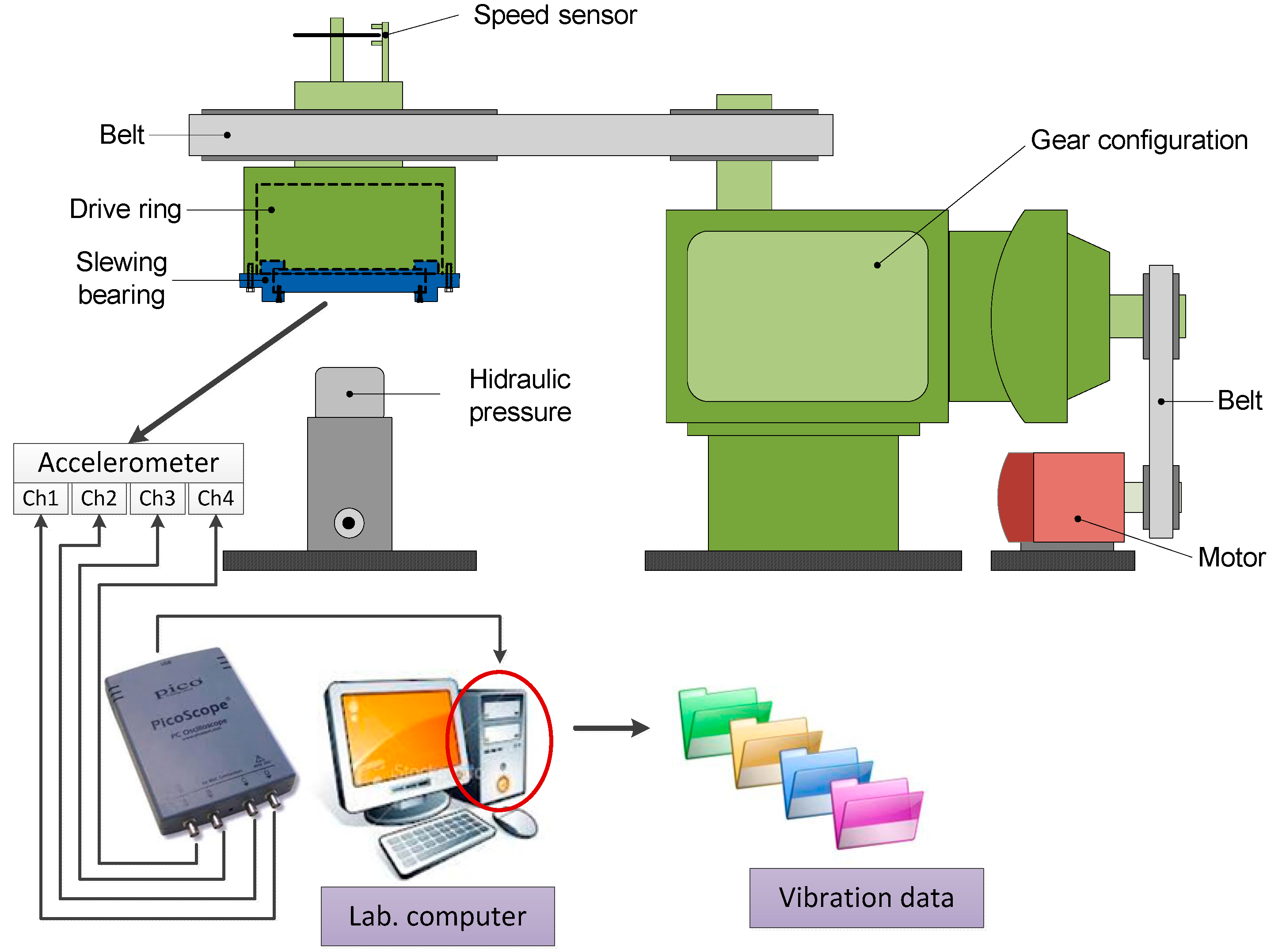
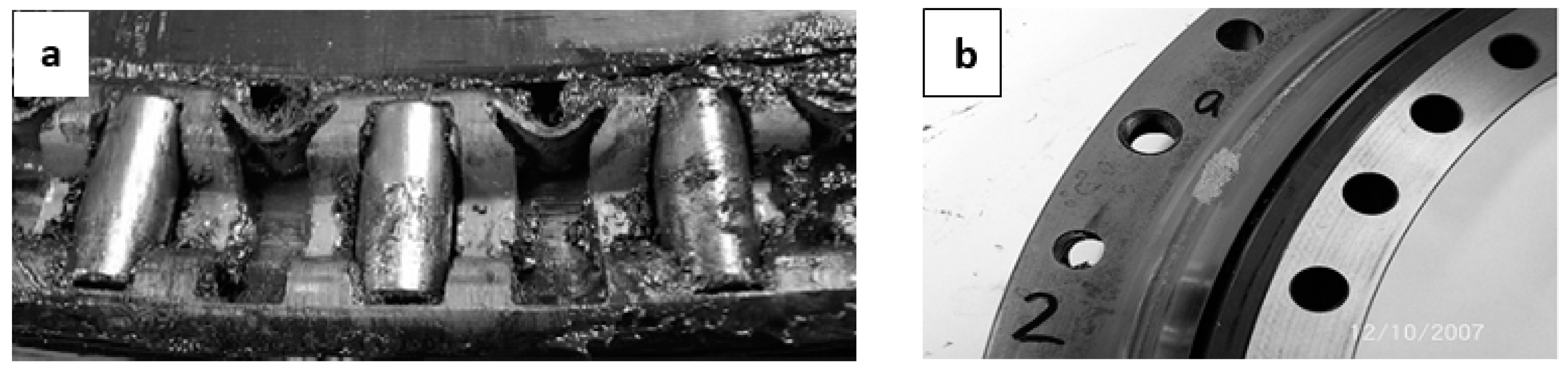
2.1. Slew Bearing Test-Rig and Sensor Location
2.2. Data Acquisition Procedure
3. Features Extraction Methods and Its Application on Slew Bearing Vibration Signal
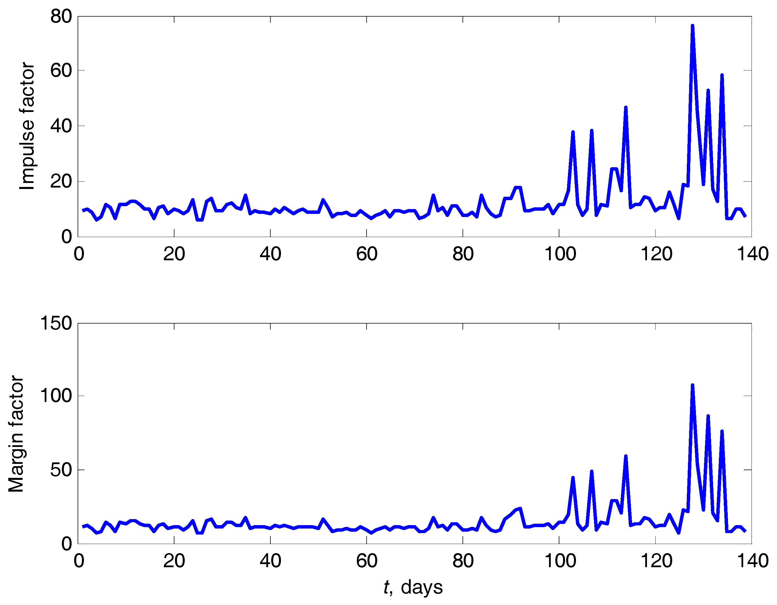
3.1. Category 1: Time-Domain Features Extraction
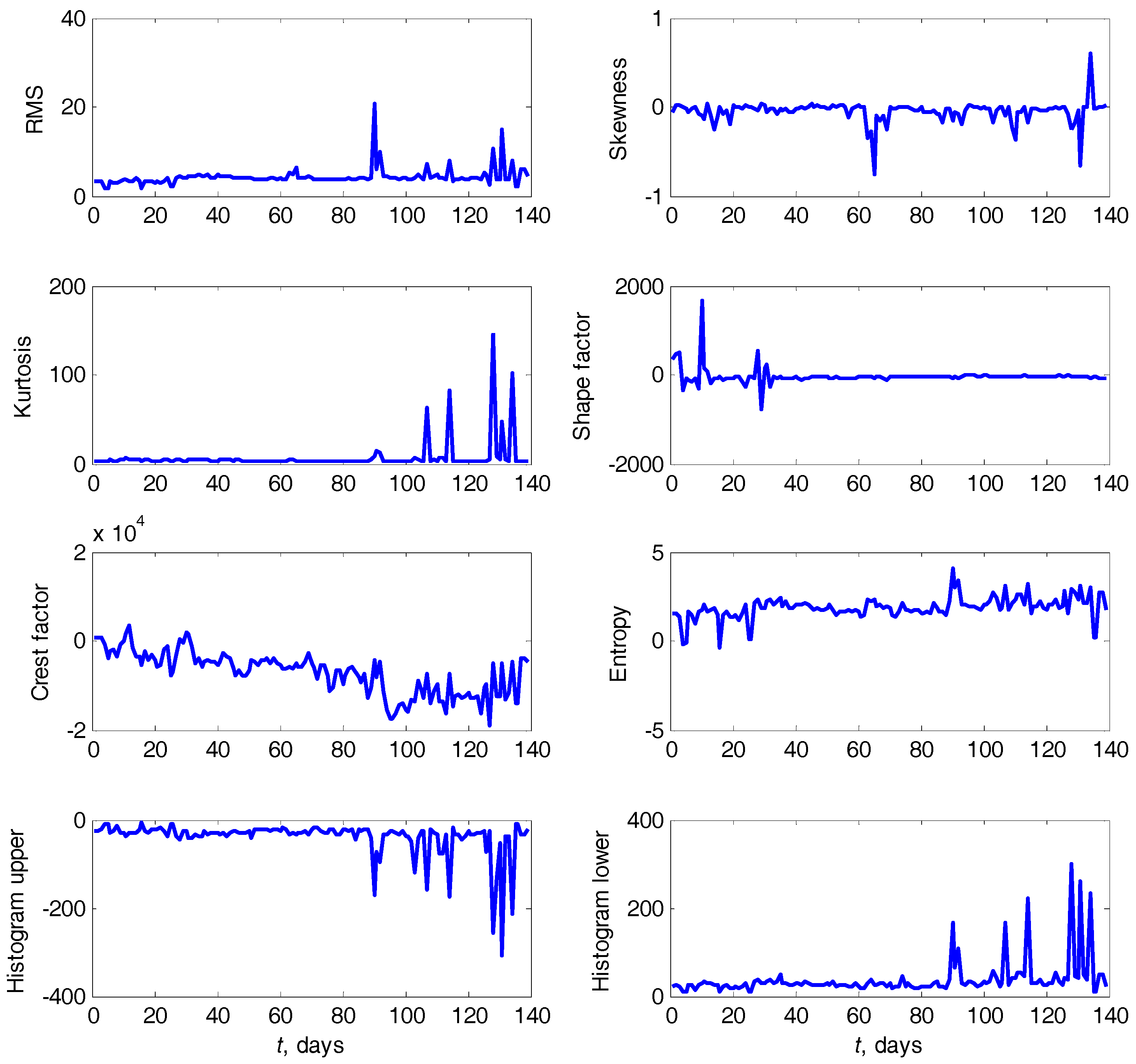
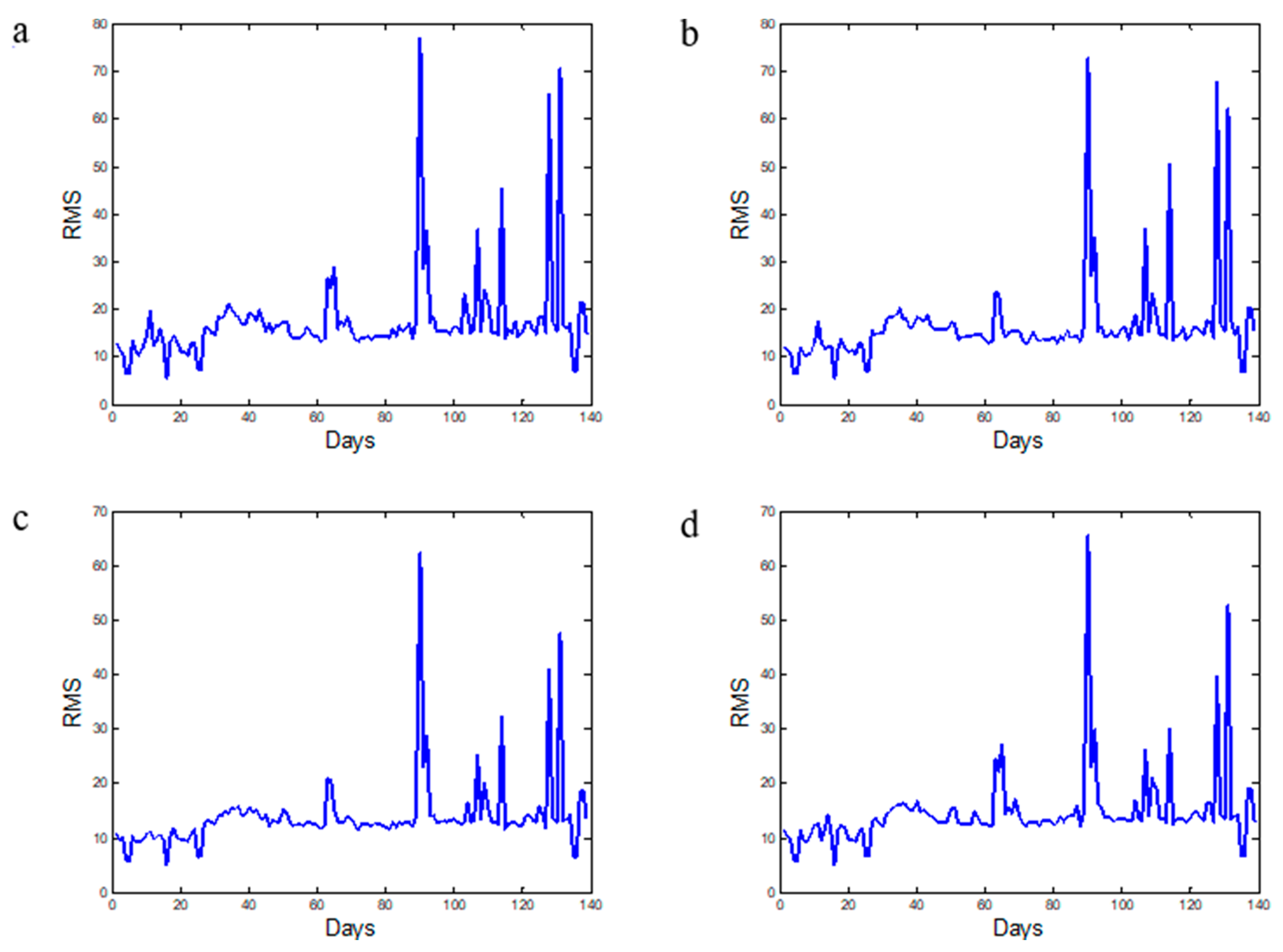
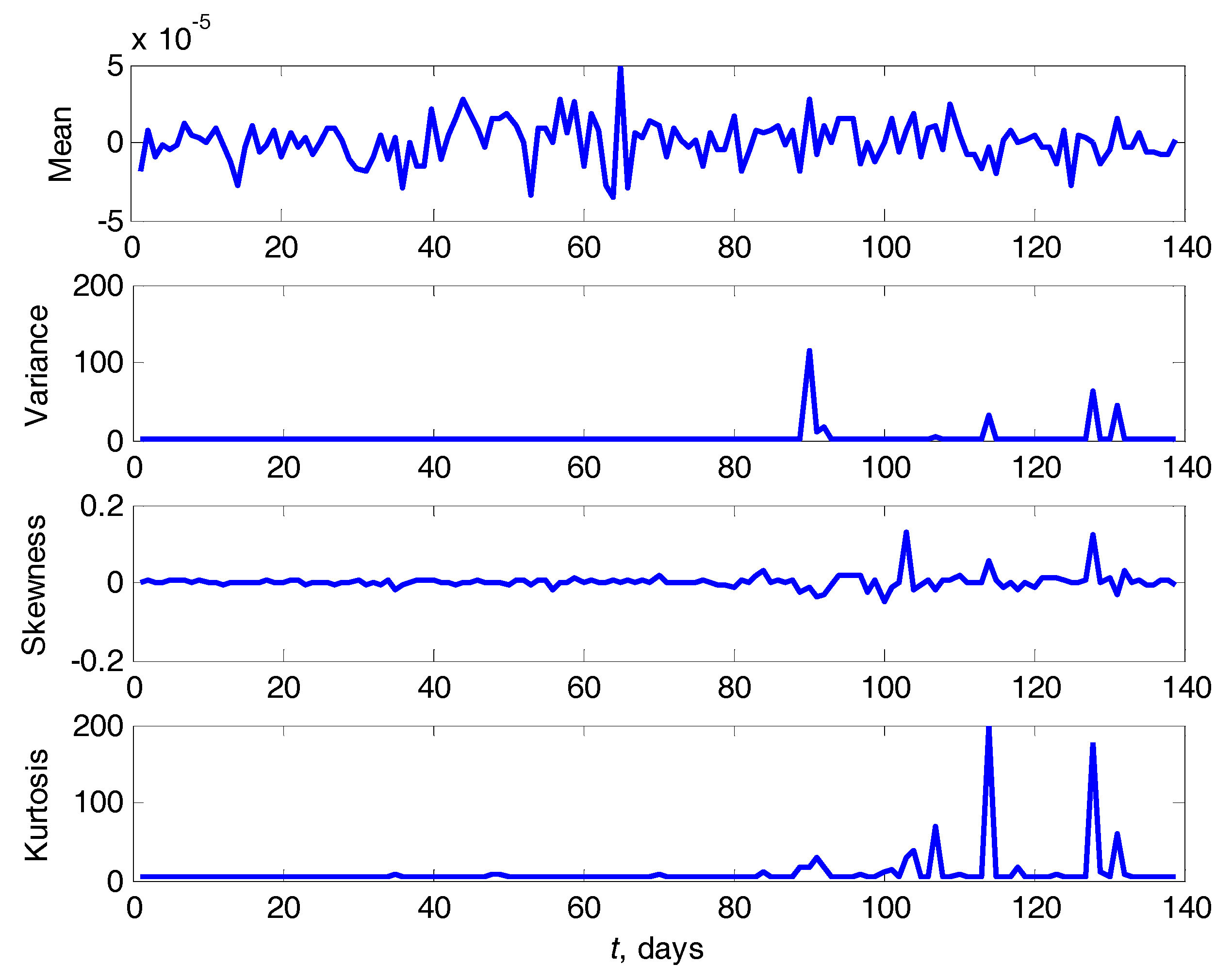
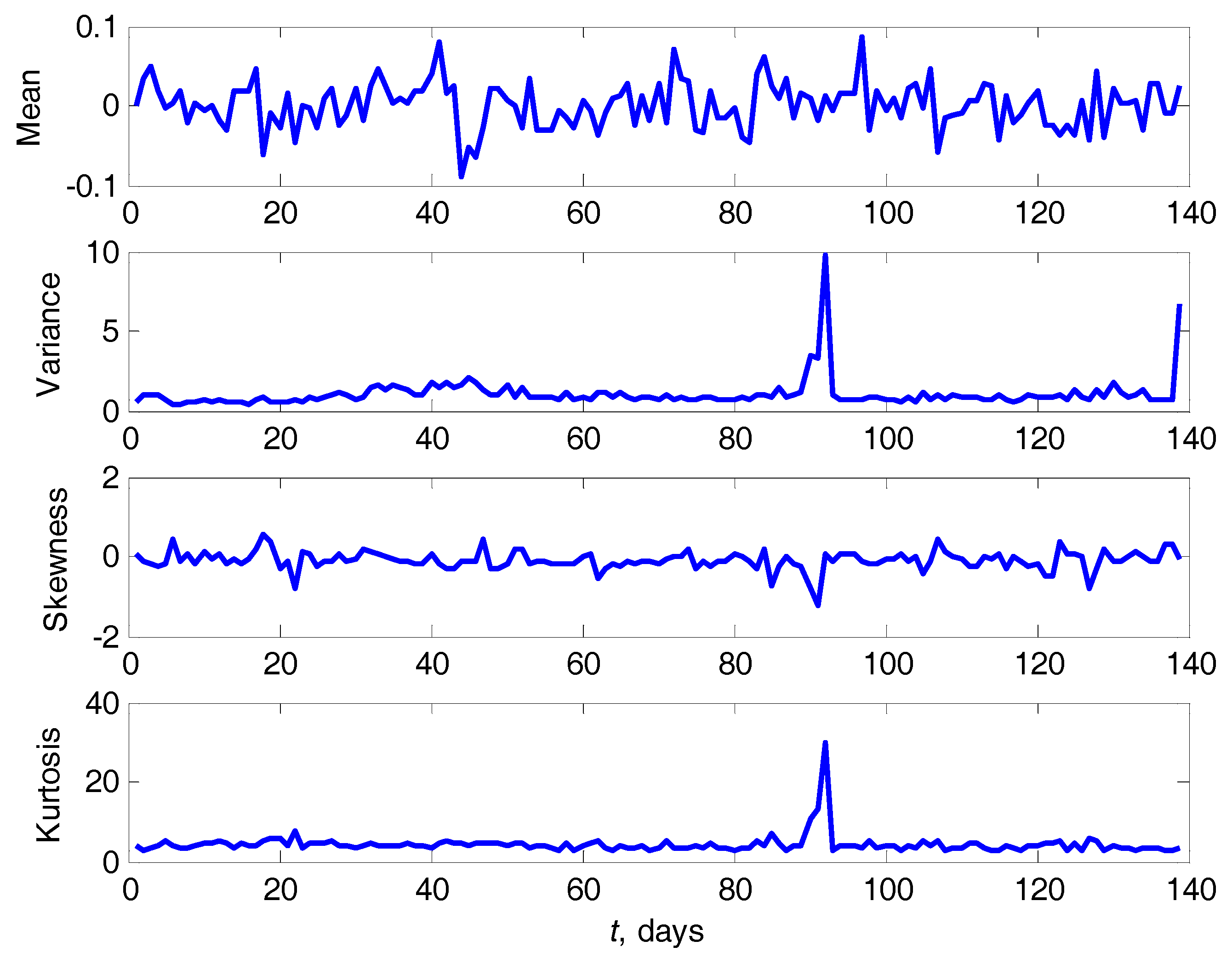
3.1.1. Statistical Time-Domain Features
3.1.2. Upper and Lower Bound of Histogram
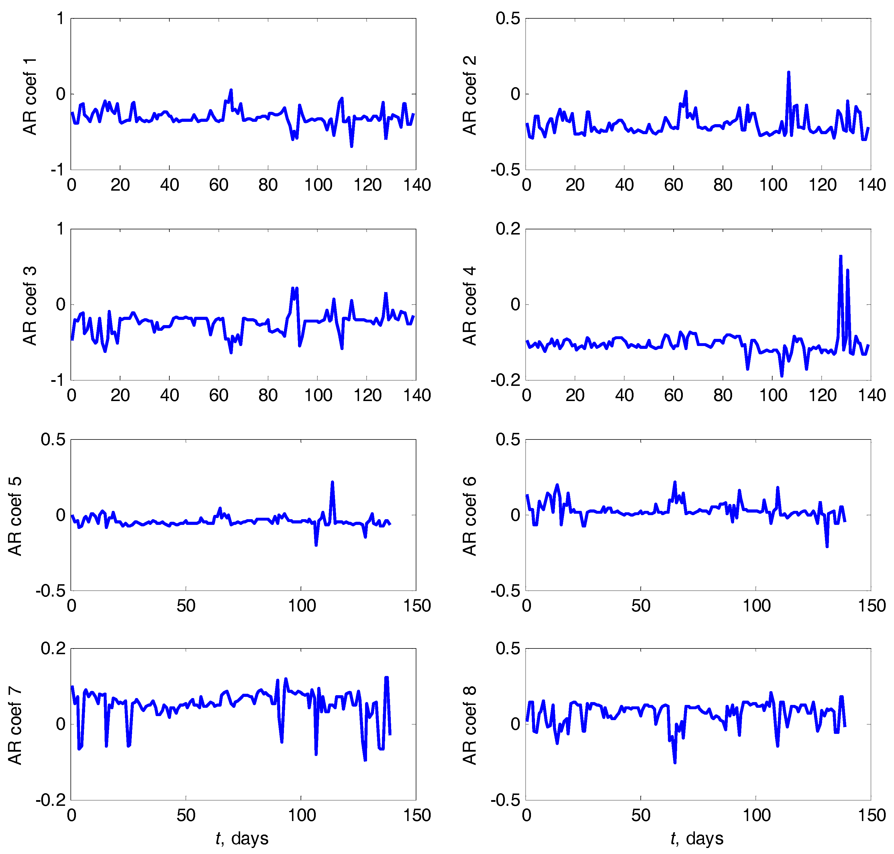
3.1.3. Autoregressive (AR) Coefficients
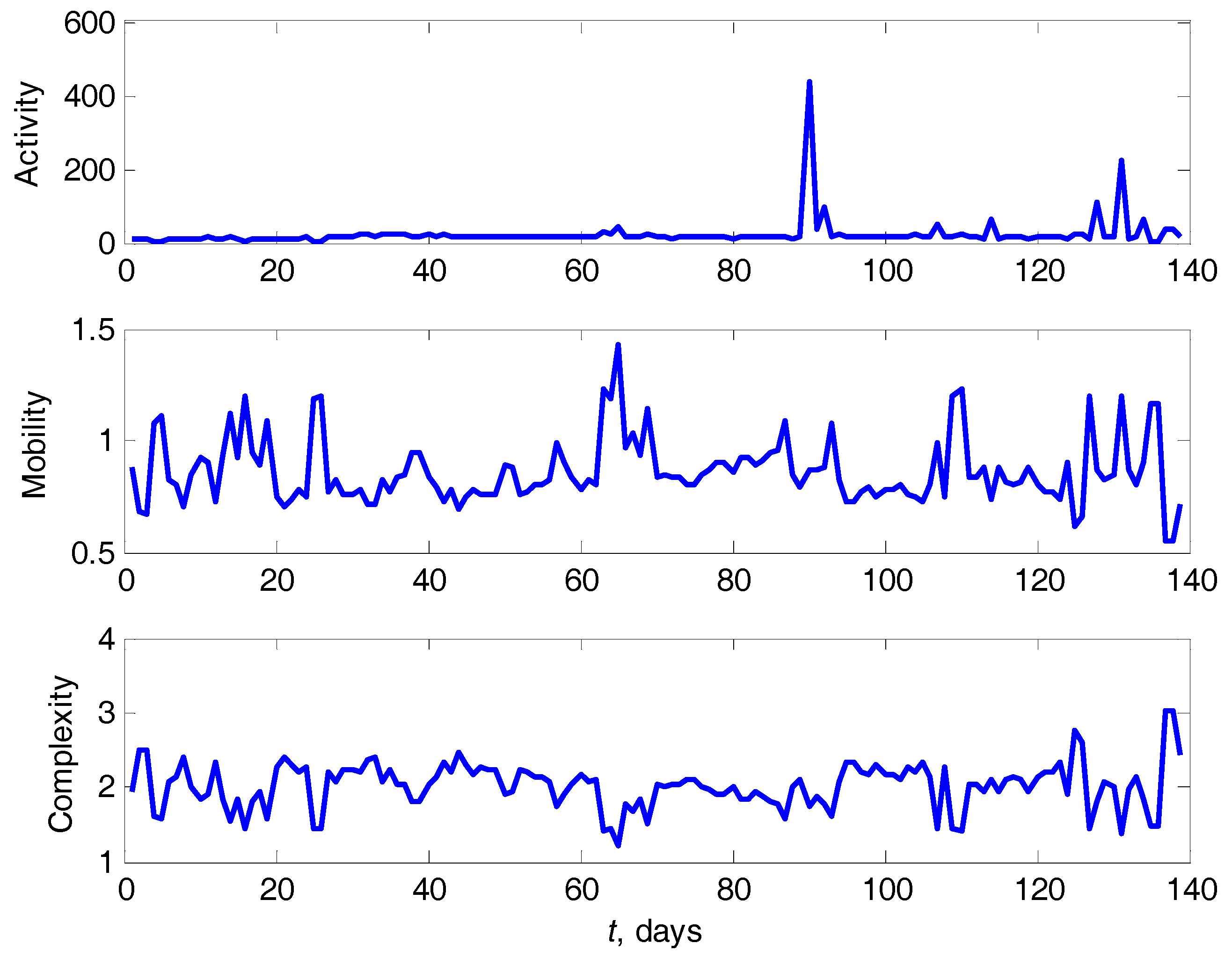
3.1.4. Hjorts’ Parameters
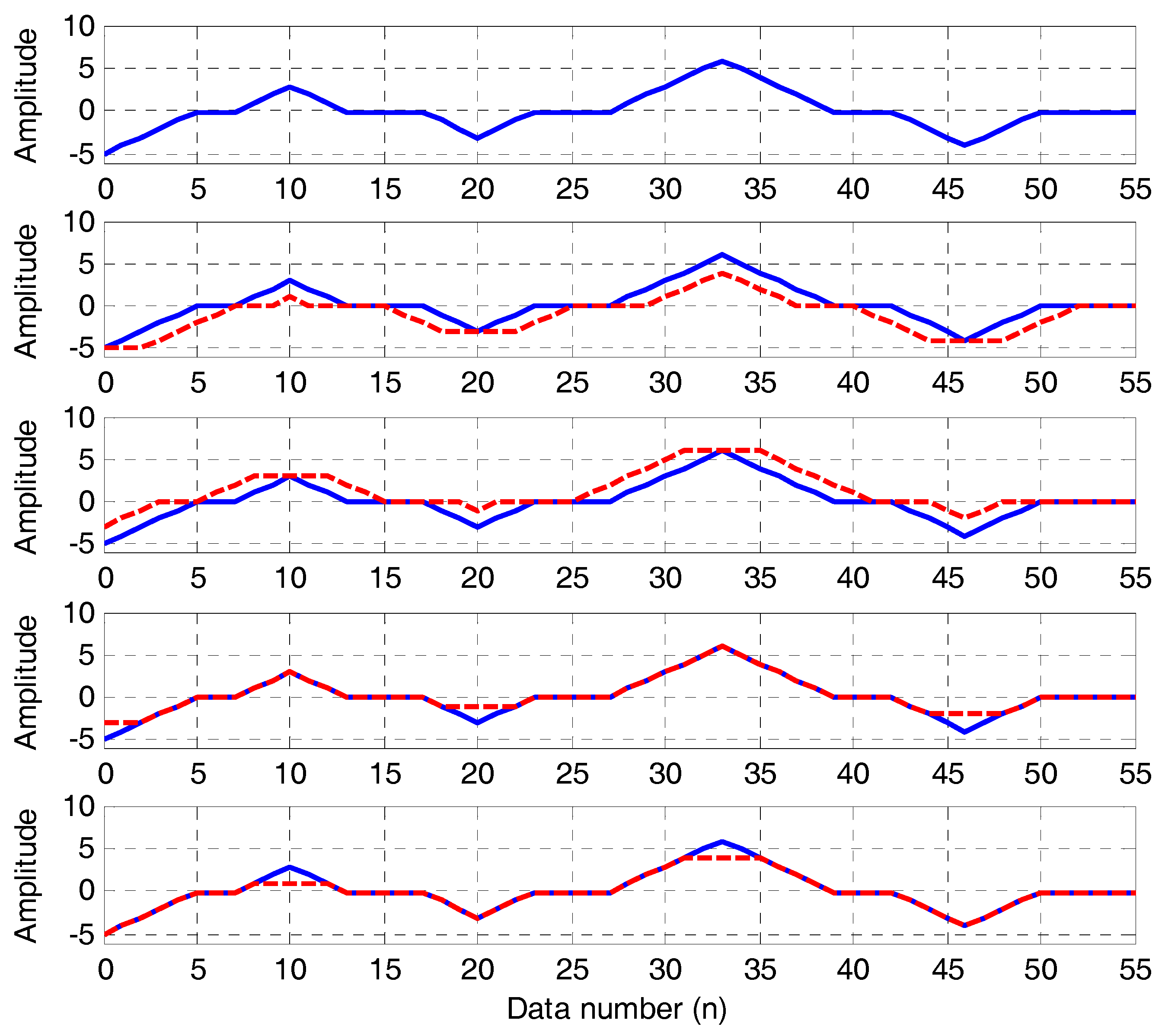
3.1.5. Mathematical Morphology (MM) Operators
- Erosion: also refer to as min filter.
- Dilation: also refer to as max filter.
- Closing: Dilates 1D signal and then erodes the dilated signal using the similar structuring element for both operations.
- Opening: Erodes 1D signal and then dilates the eroded signal using the similar structuring element for both operations.
3.2. Category 2: Frequency-Domain Features Extraction
3.2.1. Statistical Frequency-Domain Features
3.2.2. Spectral Skewness, Spectral Kurtosis, Spectral Entropy and Shannon Entropy Feature
3.3. Category 3: Time-Frequency Representation
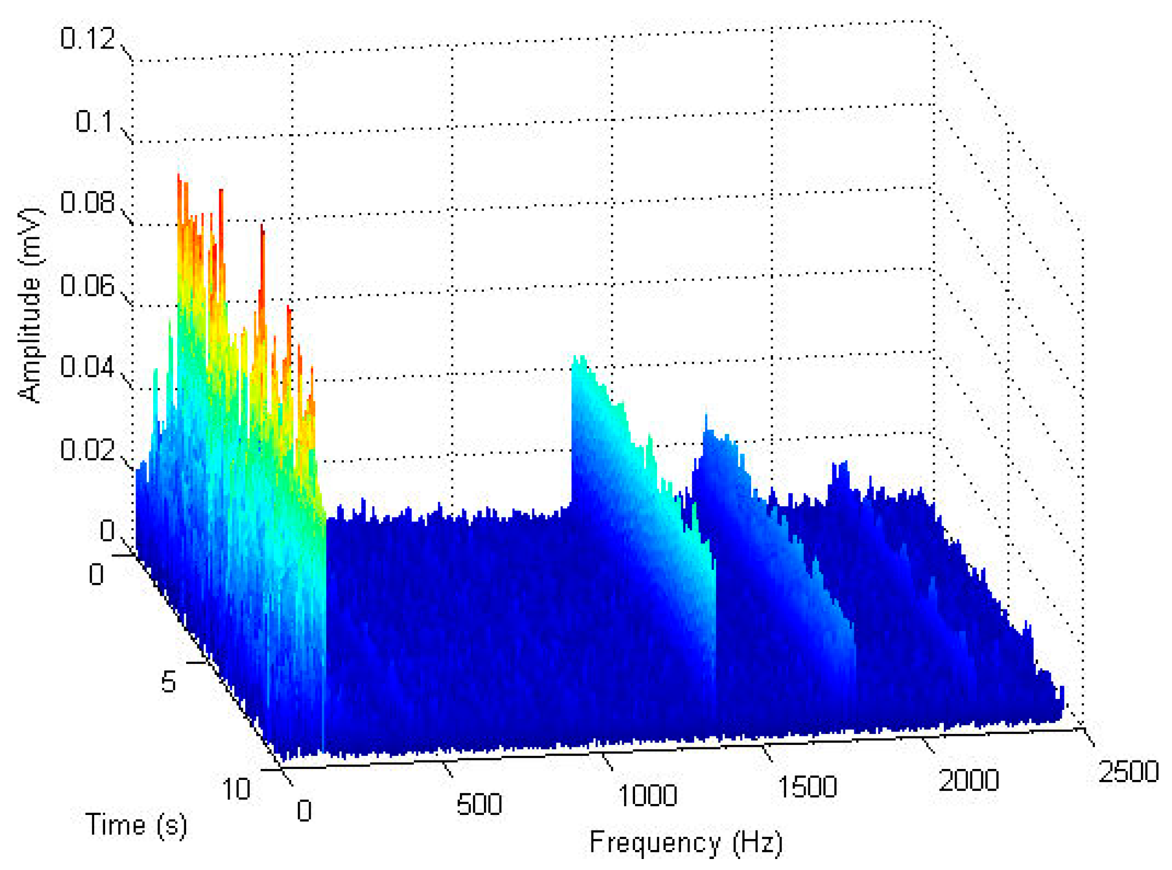
3.3.1. Short-Time Fourier Transform (STFT)
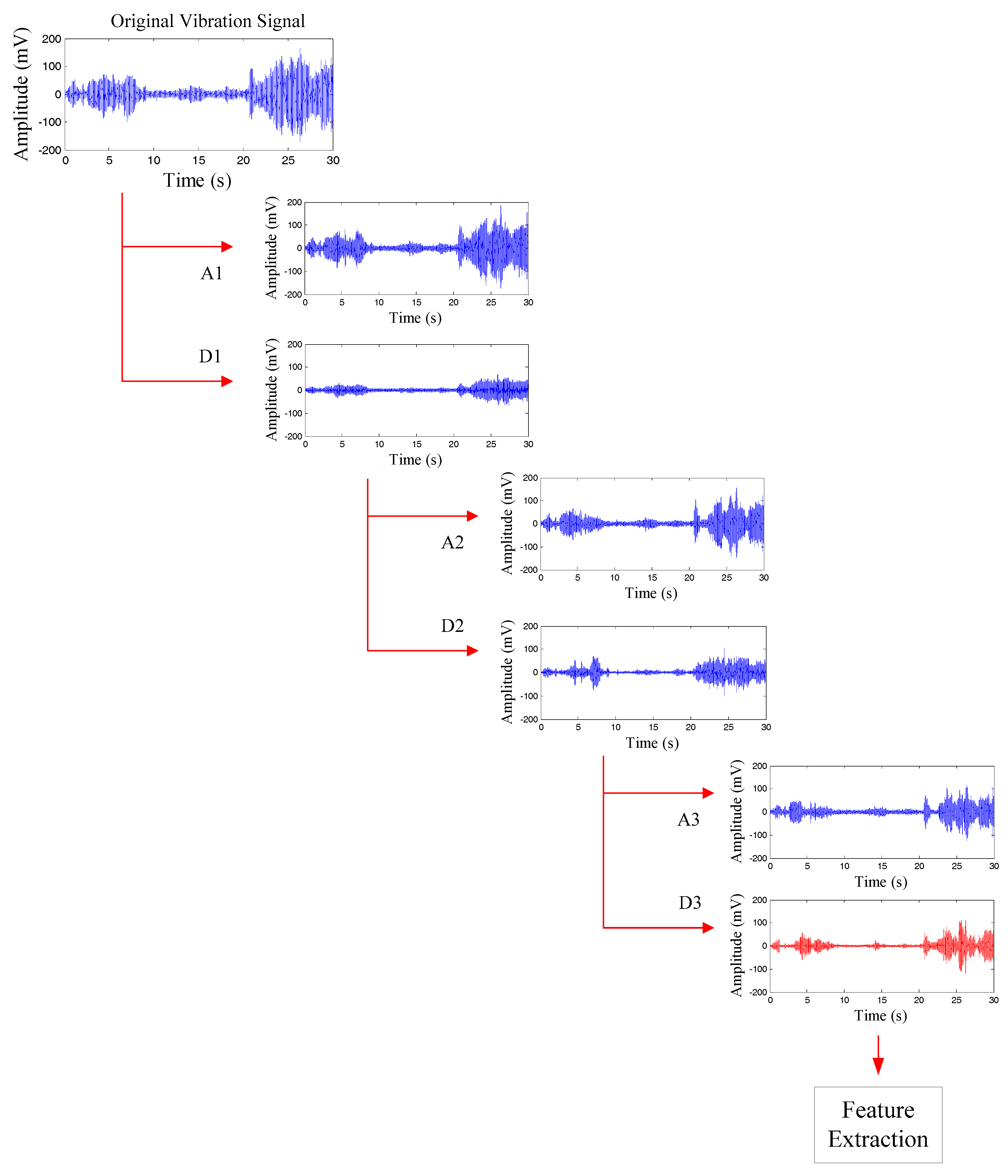
3.3.2. Wavelet Transform and Wavelet Decomposition
3.3.3. Empirical Mode Decomposition-Based Hilbert Huang Transform
3.3.4. Wigner-Ville Distribution (WVD)
3.4. Category 4: Phase-Space Dissimilarity Measurement
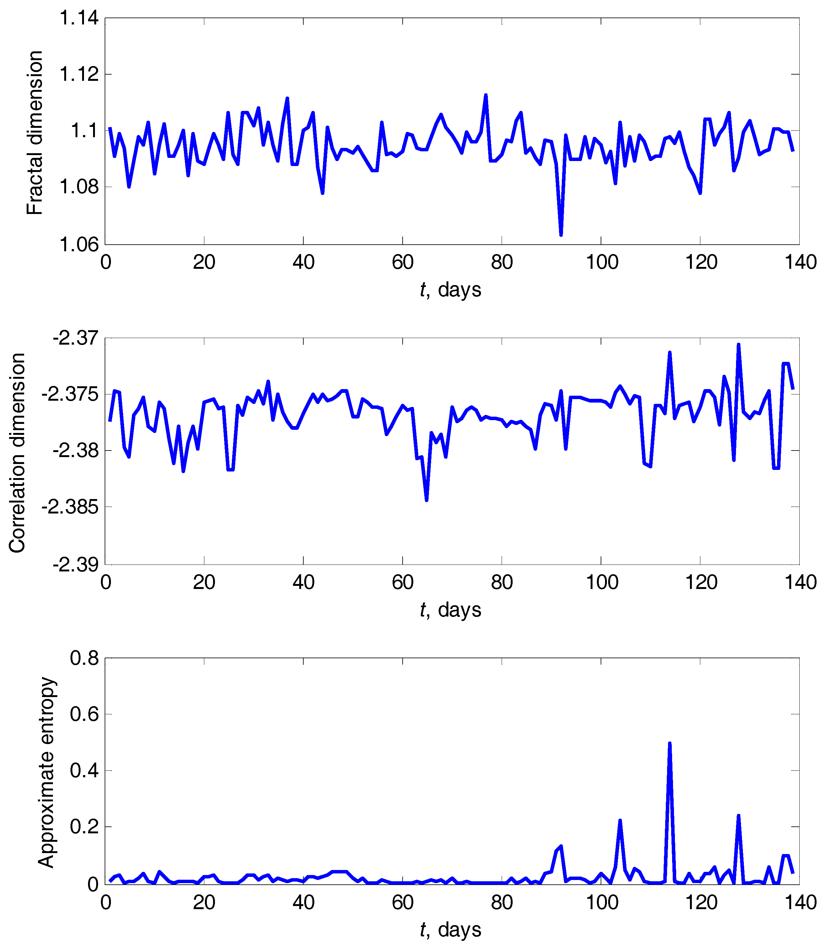
3.4.1. Fractal Dimension
3.4.2. Correlation Dimension
3.4.3. Approximate Entropy
3.4.4. Largest Lyapunov Exponent
3.5. Category 5: Complexity Measurement
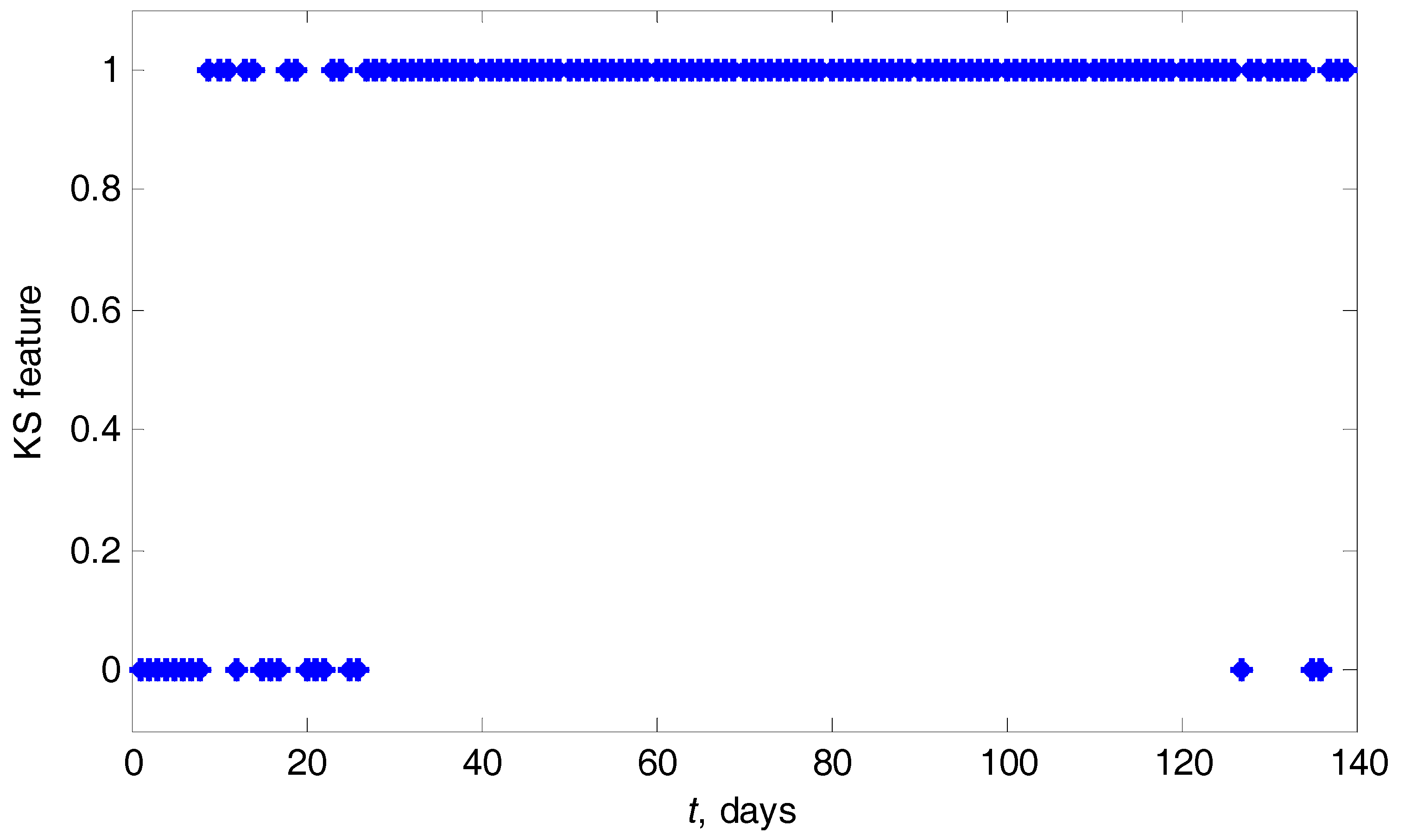
3.5.1. Kolmogorov-Smirnov Test
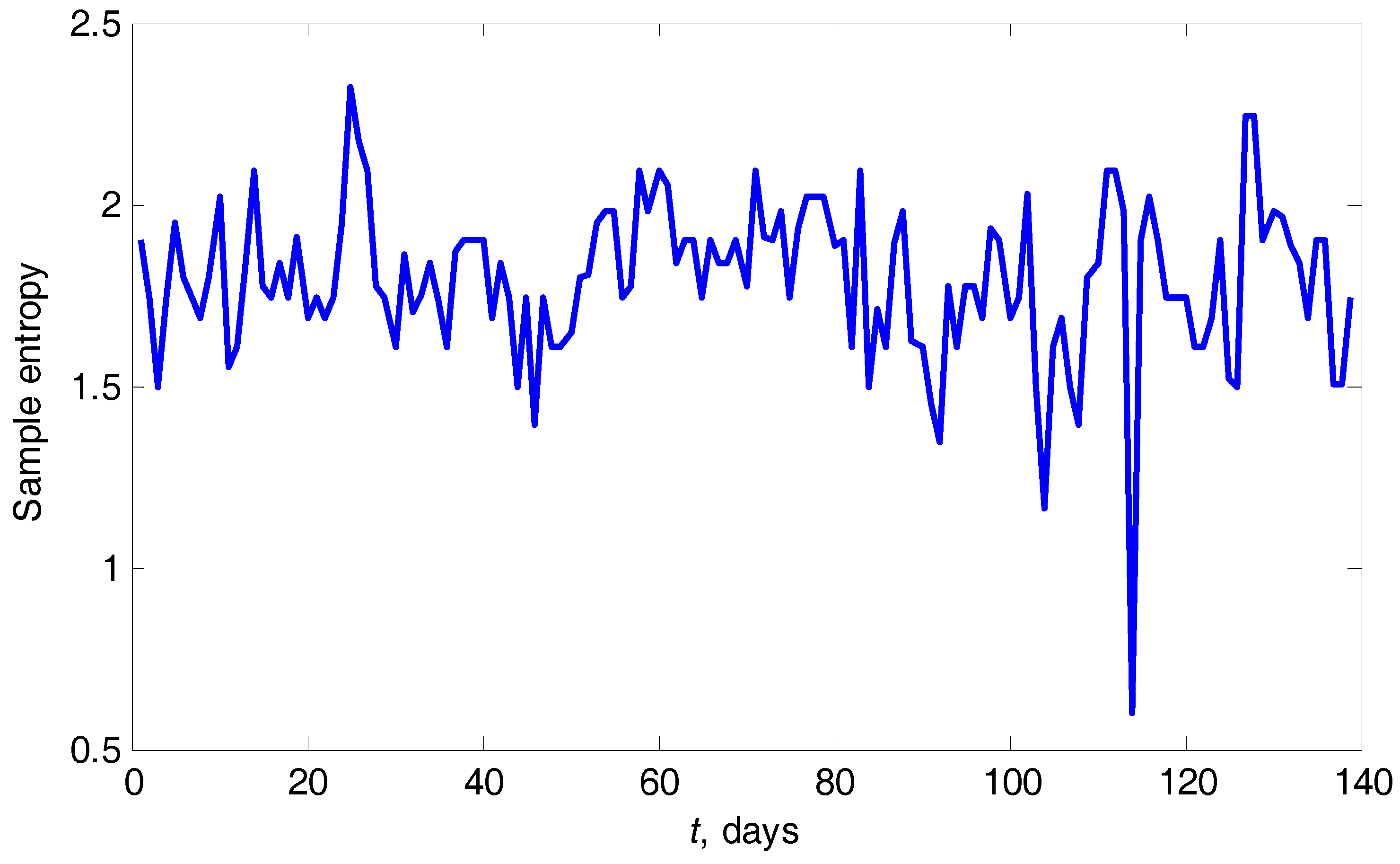
3.5.2. Sample Entropy
3.6. Category 6: Other Features
3.6.1. Singular Value Decomposition (SVD)
3.6.2. Piecewise Aggregate Approximation (PAA) and Adaptive Piecewise Constant Approximation (APCA)
4. Conclusions
Acknowledgments
Author Contributions
Conflicts of Interest
Appendix A. The Formula for Calculating Bearing Fault Frequencies [75]
- Fault frequency of outer ring:
- Fault frequency of inner ring:
- Fault frequency of rolling element:
References
- Caesarendra, W. Vibration and Acoustic Emission-Based Condition Monitoring and Prognostic Methods for Very Low Speed Slew Bearing. Ph.D. Thesis, University of Wollongong, Wollongong, Australia, 2015. [Google Scholar]
- Žvokelj, M.; Zupan, S.; Prebil, I. Multivariate and multiscale monitoring of large-size low-speed bearings using ensemble empirical mode decomposition method combined with principal component analysis. Mech. Syst. Signal Process. 2010, 24, 1049–1067. [Google Scholar] [CrossRef]
- Žvokelj, M.; Zupan, S.; Prebil, I. Non-linear multivariate and multiscale monitoring and signal denoising strategy using kernel principal component analysis combined with ensemble empirical mode decomposition method. Mech. Syst. Signal Process. 2011, 24, 2631–2653. [Google Scholar] [CrossRef]
- Žvokelj, M.; Zupan, S.; Prebil, I. EEMD-based multiscale ICA method for slewing bearing fault detection and diagnosis. J. Sound Vib. 2016, 370, 394–423. [Google Scholar] [CrossRef]
- Feng, Y.; Huang, X.; Chen, J.; Wang, H.; Hong, R. Reliability-based residual life prediction of large-size low-speed slewing bearings. Mech. Mach. Theory 2014, 81, 94–106. [Google Scholar] [CrossRef]
- Lu, C.; Chen, J.; Hong, R.; Feng, Y.; Li, Y. Degradation trend estimation of slewing bearing based on LSSVM model. Mech. Syst. Signal Process. 2016, 76–77, 353–366. [Google Scholar] [CrossRef]
- Hua, W.; Yan, T.; Rongjing, H. Multiple physical signals based residual life prediction model of slewing bearing. J. Vibroeng. 2016, 18, 4340–4353. [Google Scholar]
- Henao, H.; Capolino, G.A.; Fernandez-Cabanas, M.; Filippetti, F.; Bruzzese, C.; Strangas, E.; Pusca, R.; Estima, J.; Riera-Guasp, M.; Hedayati-Kia, S. Trends in fault diagnosis for electrical machines: A review of diagnostic techniques. IEEE Ind. Electron. Mag. 2014, 8, 31–42. [Google Scholar] [CrossRef]
- Eftekharnejad, B.; Carrasco, M.R.; Charnley, B.; Mba, D. The application of spectral kurtosis on Acoustic Emission and vibrations from a defective bearing. Mech. Syst. Signal Process. 2011, 25, 266–284. [Google Scholar] [CrossRef] [Green Version]
- Caesarendra, W.; Kosasih, B.; Tieu, K.; Moodie, C.A.S. An Application of Nonlinear Feature Extraction—A Case Study for Low Speed Slewing Bearing Condition Monitoring and Prognosis. In Proceedings of the IEEE/ASME International Conference on Advanced Intelligent Mechatronics (AIM), Wollongong, Australia, 9–12 July 2013. [Google Scholar]
- Shen, K.; He, Z.; Chen, X.; Sun, C.; Liu, Z. A monotonic degradation assessment index of rolling bearings using fuzzy support vector data description and running time. Sensors 2012, 12, 10109–10135. [Google Scholar] [CrossRef] [PubMed]
- Yiakopoulos, C.T.; Gryllias, K.C.; Antoniadis, I.A. Rolling element bearing fault detection in industrial environments based on a K-means clustering approach. Expert Syst. Appl. 2011, 38, 2888–2911. [Google Scholar] [CrossRef]
- Yang, B.S.; Widodo, A. Introduction of Intelligent Machine Fault Diagnosis and Prognosis; Nova Science Publishers: New York, NY, USA, 2009. [Google Scholar]
- Widodo, A.; Yang, B.S. Wavelet support vector machine for induction machine fault diagnosis based on transient current signal. Expert Syst. Appl. 2008, 35, 307–316. [Google Scholar] [CrossRef]
- Widodo, A.; Kim, E.Y.; Son, J.D.; Yang, B.S.; Tan, A.C.C.; Gu, D.S.; Choi, B.K.; Mathew, J. Fault diagnosis of low speed bearing based on relevance vector machine and support vector machine. Expert Syst. Appl. 2009, 36, 7252–7261. [Google Scholar] [CrossRef]
- Yu, J. Bearing performance degradation assessment using locality preserving projections and Gaussian mixture models. Mech. Syst. Signal Process. 2011, 25, 2573–2588. [Google Scholar] [CrossRef]
- Xia, Z.; Xia, S.; Wan, L.; Cai, S. Spectral regression based fault feature extraction for bearing accelerometer sensor signals. Sensors 2012, 12, 13694–13719. [Google Scholar] [CrossRef] [PubMed]
- Rangayyan, R.M. Biomedical Signal Analysis: A Case-Study Approach; Wiley: New York, NY, USA, 2002. [Google Scholar]
- Päivinen, N.; Lammi, S.; Pitkanen, A.; Nissinen, J.; Penttonen, M.; Grӧnfors, T. Epileptic seizure detection: A nonlinear viewpoint. Comput. Methods Programs Biomed. 2005, 79, 151–159. [Google Scholar] [CrossRef] [PubMed]
- Serra, J. Image Analysis and Mathematical Morphology; Academic Press: New York, NY, USA, 1982. [Google Scholar]
- Nishida, S.; Nakamura, M.; Miyazaki, M.; Suwazono, S.; Honda, M.; Nagamine, T.; Shibazaki, H. Construction of a morphological filter for detecting an event related potential P300 in single sweep EEG record in children. Med. Eng. Phys. 1995, 17, 425–430. [Google Scholar] [CrossRef]
- Nishida, S.; Nakamura, M.; Shindo, K.; Kanda, M.; Shibazaki, H. A morphological filter for extracting waveform characteristics of single sweep evoked potentials. Automatica 1997, 35, 937–943. [Google Scholar] [CrossRef]
- Nishida, S.; Nakamura, M.; Ikeda, A.; Shibazaki, H. Signal separation of background EEG and spike by using morphological filter. Med. Eng. Phys. 1999, 21, 601–608. [Google Scholar] [CrossRef]
- Sedaaghi, M.H. ECG wave detection using morphological filters. Appl. Signal Process. 1998, 5, 182–194. [Google Scholar] [CrossRef]
- Nikolaou, N.G.; Antoniadis, I.A. Application of morphological operators as envelope extractors for impulsive-type periodic signals. Mech. Syst. Signal Process. 2003, 17, 1147–1162. [Google Scholar] [CrossRef]
- Zhang, L.; Xu, J.; Yang, J.; Yang, D.; Wang, D. Multiscale morphology analysis and its application to fault diagnosis. Mech. Syst. Signal Process. 2008, 22, 597–610. [Google Scholar] [CrossRef]
- Wang, J.; Xu, G.; Zhang, Q.; Liang, L. Application of improved morphological filter to the extraction of impulsive attenuation signals. Mech. Syst. Signal Process. 2009, 23, 236–245. [Google Scholar] [CrossRef]
- Dong, Y.; Liao, M.; Zhang, X.; Wang, F. Faults diagnosis of rolling element bearings based on modified morphological method. Mech. Syst. Signal Process. 2011, 25, 1276–1286. [Google Scholar] [CrossRef]
- Santhana, R.; Murali, N. Early classification of bearing faults using morphological operators and fuzzy inference. IEEE Trans. Ind. Electron. 2013, 60, 567–574. [Google Scholar]
- Drummond, C.F.; Sutanto, D. Classification of power quality disturbances using the Iterative Hilbert Huang Transform. In Proceedings of the 14th International Conference on Harmonics and Quality of Power, Bergamo, Italy, 26–29 September 2010; p. 107. [Google Scholar]
- Lerch, A. An Introduction to Audio Content Analysis: Applications in Signal Processing and Music Informatics; Wiley-IEEE Press: Hoboken, NJ, USA, 2012. [Google Scholar]
- Antoni, J.; Randall, R.B. The spectral kurtosis: Application to the vibratory surveillance and diagnostics of rotating machines. Mech. Syst. Signal Process. 2006, 20, 308–331. [Google Scholar] [CrossRef]
- Feng, Z.; Liang, M.; Chu, F. Recent advances in time-frequency analysis methods for machinery fault diagnosis: A review with application examples. Mech. Syst. Signal Process. 2013, 38, 165–205. [Google Scholar] [CrossRef]
- Al-Badour, F.; Sunar, M.; Cheded, L. Vibration analysis of rotating machinery using time-frequency analysis and wavelet techniques. Mech. Syst. Signal Process. 2011, 25, 2083–2101. [Google Scholar] [CrossRef]
- Allen, J.B. Short term spectral analysis, synthesis, and modification by discrete Fourier transform. IEEE Trans. Acoust. Speech Signal Process. 1977, 25, 235–238. [Google Scholar] [CrossRef]
- Wang, S.; Huang, W.; Zhu, Z.K. Transient modeling and parameter identification based on wavelet and correlation filtering for rotating machine fault diagnosis. Mech. Syst. Signal Process. 2011, 25, 1299–1320. [Google Scholar] [CrossRef]
- Peng, Z.K.; Chu, F.L. Application of the wavelet transform in machine condition monitoring and fault diagnostics: A review with bibliography. Mech. Syst. Signal Process. 2004, 18, 199–221. [Google Scholar] [CrossRef]
- Daubechies, C.I. Ten Lectures on Wavelet; SIAM: Philadelphia, PA, USA, 1992. [Google Scholar]
- Caesarendra, W.; Kosasih, B.; Tieu, A.K.; Moodie, C.A.S. Circular domain features based condition monitoring for low speed slewing bearing. Mech. Syst. Signal Process. 2014, 45, 114–138. [Google Scholar] [CrossRef]
- Niu, G.; Widodo, A.; Son, J.D.; Yang, B.S.; Hwang, D.H.; Kang, D.S. Decision-level fusion based on wavelet decomposition for induction motor fault diagnosis using transient current signal. Expert Syst. Appl. 2008, 35, 918–928. [Google Scholar] [CrossRef]
- Liu, B.; Ling, S.F.; Meng, Q. Machinery diagnosis based on wavelets packets. J. Vib. Control 1997, 3, 5–17. [Google Scholar]
- Huang, N.E.; Shen, Z.; Long, S.R.; Wu, M.C.; Shih, H.H.; Zheng, Q.; Yen, N.C.; Tung, C.C.; Liu, H.H. The empirical mode decomposition and the Hilbert spectrum for nonlinear and non-stationary time series analysis. Proc. R. Soc. Lond. A 1998, 454, 903–995. [Google Scholar] [CrossRef]
- Braun, S.; Feldman, M. Decomposition of non-stationary signals into varying time scales: Some aspects of the EMD and HVD methods. Mech. Syst. Signal Process. 2011, 25, 2608–2630. [Google Scholar] [CrossRef]
- Lei, Y.; Lin, J.; He, Z.; Zuo, M.J. A review on empirical mode decomposition in fault diagnosis of rotating machinery. Mech. Syst. Signal Process. 2013, 35, 108–126. [Google Scholar] [CrossRef]
- Caesarendra, W.; Kosasih, P.B.; Tieu, A.K.; Moodie, C.A.S.; Choi, B.K. Condition monitoring of naturally damaged slow speed slewing bearing based on ensemble empirical mode decomposition. J. Mech. Sci. Technol. 2013, 27, 1–10. [Google Scholar] [CrossRef]
- Rilling, G.; Flandrin, P.; Gonçalves, P. On empirical mode decomposition and its algorithms. In Proceedings of the IEEE-EURASiP Workshop on Nonlinear Signal and Image Processing, Grado, Italy, 8–11 June 2003. [Google Scholar]
- Staszewski, W.J.; Worden, K.; Tomlinson, G.R. Time-frequency analysis in gearbox fault detection using the Wigner-Ville distribution and pattern recognition. Mech. Syst. Signal Process. 1997, 11, 673–692. [Google Scholar] [CrossRef]
- Loutridis, S.J. Instantaneous energy density as a feature for gear fault detection. Mech. Syst. Signal Process. 2006, 20, 1239–1253. [Google Scholar] [CrossRef]
- Claasen, T.A.M.; Mecklenbrauker, W.F.G. The Wigner distribution—A tool for time-frequency analysis. Part 1: Continuous time signals. Philips J. Res. 1980, 35, 217–250. [Google Scholar]
- Dong, G.; Chen, J. Noise resistant time frequency analysis and application in fault diagnosis of rolling element bearings. Mech. Syst. Signal Process. 2012, 33, 212–236. [Google Scholar] [CrossRef]
- Ubeyli, E.D. Adaptive neuro-fuzzy inference system for classification of EEG signals using Lyapunov exponents. Comput. Methods Programs Biomed. 2009, 93, 313–321. [Google Scholar] [CrossRef] [PubMed]
- Logan, D.; Mathew, J. Using the correlation dimension for vibration fault diagnosis of rolling element bearings-I. Basics concepts. Mech. Syst. Signal Process. 1996, 10, 241–250. [Google Scholar] [CrossRef]
- Lu, C.; Sun, Q.; Tao, L.; Liu, H.; Lu, C. Bearing health assessment based on chaotic characteristics. Shock Vib. 2013, 20, 519–530. [Google Scholar] [CrossRef]
- Higuchi, T. Relationship between the fractal dimension and the power law index for a time series: A numerical investigation. Phys. D Nonlinear Phenom. 1990, 46, 254–264. [Google Scholar] [CrossRef]
- N’Diaye, M.; Degeratu, C.; Bouler, J.M.; Chappard, D. Biomaterial porosity determined by fractal dimensions, succolarity and lacunarity on microcomputed tomographic images. Mater. Sci. Eng. C 2013, 33, 2025–2030. [Google Scholar] [CrossRef] [PubMed] [Green Version]
- Accardo, A.; Affinito, M.; Carrozi, M.; Bouquet, F. Use of the fractal dimension for the analysis of electroencephalographic time series. Biol. Cybern. 1997, 77, 339–350. [Google Scholar] [PubMed]
- King, R.D.; George, A.T.; Jeon, T.; Hynan, L.S.; Youn, T.S.; Kennedy, D.N.; Dickerson, B.; Alzheimer’s Disease Neuroimaging Initiative. Characterization of atrophic changes in the cerebral cortex using fractal dimensional analysis. Brain Imaging Behav. 2009, 3, 154–166. [Google Scholar] [CrossRef] [PubMed]
- Liu, J.Z.; Zhang, L.D.; Yue, G.H. Fractal dimension in human Cerebellum measured by magnetic resonance imaging. Biophys. J. 2003, 85, 4041–4046. [Google Scholar] [CrossRef]
- Roberts, A.J.; Cronin, A. Unbiased estimation of multi-fractal dimensions of finite data sets. Phys. A Stat. Mech. Appl. 1996, 233, 867–878. [Google Scholar] [CrossRef]
- Maragos, P.; Potamianos, A. Fractal dimensions of speech sounds: Computation and application to automatic speech recognition. J. Acoust. Soc. Am. 1999, 105, 1925–1932. [Google Scholar] [CrossRef] [PubMed]
- Yang, J.; Zhang, Y.; Zhu, Y. Intelligent fault diagnosis of rolling element bearing based on SVMs and fractal dimension. Mech. Syst. Signal Process. 2007, 21, 2012–2024. [Google Scholar] [CrossRef]
- Grassberger, P.; Procaccia, I. Estimation of the Kolmogorov entropy from a chaotic signal. Phys. Rev. A 1983, 28, 2591–2593. [Google Scholar] [CrossRef]
- Yan, R.; Gao, R.X. Approximate entropy as a diagnostic tool for machine health monitoring. Mech. Syst. Signal Process. 2007, 21, 824–839. [Google Scholar] [CrossRef]
- Caesarendra, W.; Kosasih, B.; Tieu, A.K.; Moodie, C.A.S. Application of the largest Lyapunov exponent algorithm for feature extraction in low speed slew bearing condition monitorin. Mech. Syst. Signal Process. 2005, 50, 116–138. [Google Scholar]
- Cong, F.; Chen, J.; Pan, Y. Kolmogorov-Smirnov test for rolling bearing performance degradation assessment and prognosis. J. Vib. Control 2011, 17, 1337–1347. [Google Scholar] [CrossRef]
- Richman, J.S.; Moorman, J.R. Physiological time-series analysis using approximate entropy and sample entropy. Am. J. Physiol. Heart Circ. Physiol. 2000, 278, H2039–H2049. [Google Scholar] [PubMed]
- Chen, X.; Yin, C.; He, W. Feature extraction of gearbox vibration signals based on EEMD and sample entropy. In Proceedings of the 10th International Conference on Fuzzy Systems and Knowledge Discovery (FSKD), Shenyang, China, 23–25 July 2013; pp. 811–815. [Google Scholar]
- Wong, M.L.D.; Liu, C.; Nandi, A.K. Classification of ball bearing faults using entropic measures. Surveillance 2013, 7, 1–8. [Google Scholar]
- Kanjilal, P.P.; Palit, S. On multiple pattern extraction using singular value decomposition. IEEE Trans. Signal Process. 1995, 43, 1536–1540. [Google Scholar] [CrossRef]
- Kanjilal, P.P.; Bhattacharya, J.; Saha, G. Robust method for periodicity detection and characterization of irregular cyclical series in term of embedded periodic components. Phys. Rev. E 1999, 59, 4013–4025. [Google Scholar] [CrossRef]
- Qiu, H.; Lee, J.; Lin, J.; Yu, G. Wavelet filter-based weak signature detection method and its application on rolling element bearing prognostics. J. Sound Vib. 2006, 289, 1066–1090. [Google Scholar] [CrossRef]
- Keogh, E.; Chakrabarti, K.; Pazzani, M.; Mehrotra, S. Dimensionality reduction for fast similarity search in large time series databases. Knowl. Inf. Syst. 2001, 3, 263–286. [Google Scholar] [CrossRef]
- Yi, B.K.; Faloutsos, C. Fast time sequence indexing for arbitrary Lp norms. In Proceedings of the 26th International Conference on Very Large Data Bases Cairo (VLDB ’00), Cairo, Egypt, 10–14 September 2000; pp. 385–394. [Google Scholar]
- Chakrabarti, K.; Keogh, E.; Mehrotra, S.; Pazzani, M. Locally adaptive dimensionality reduction for indexing large time series databases. ACM Trans. Database Syst. 2002, 27, 188–228. [Google Scholar] [CrossRef]
- Eschmann, P.; Hasbargen, L.; Weigand, K. Die Wälzlagerpraxis: Handbuch für die Berechnung und Gestaltung von Lagerungen; R. Oldenburg: München, Germany, 1953. [Google Scholar]


| Feature Name | Description | |
|---|---|---|
| Brief Definition | Formula | |
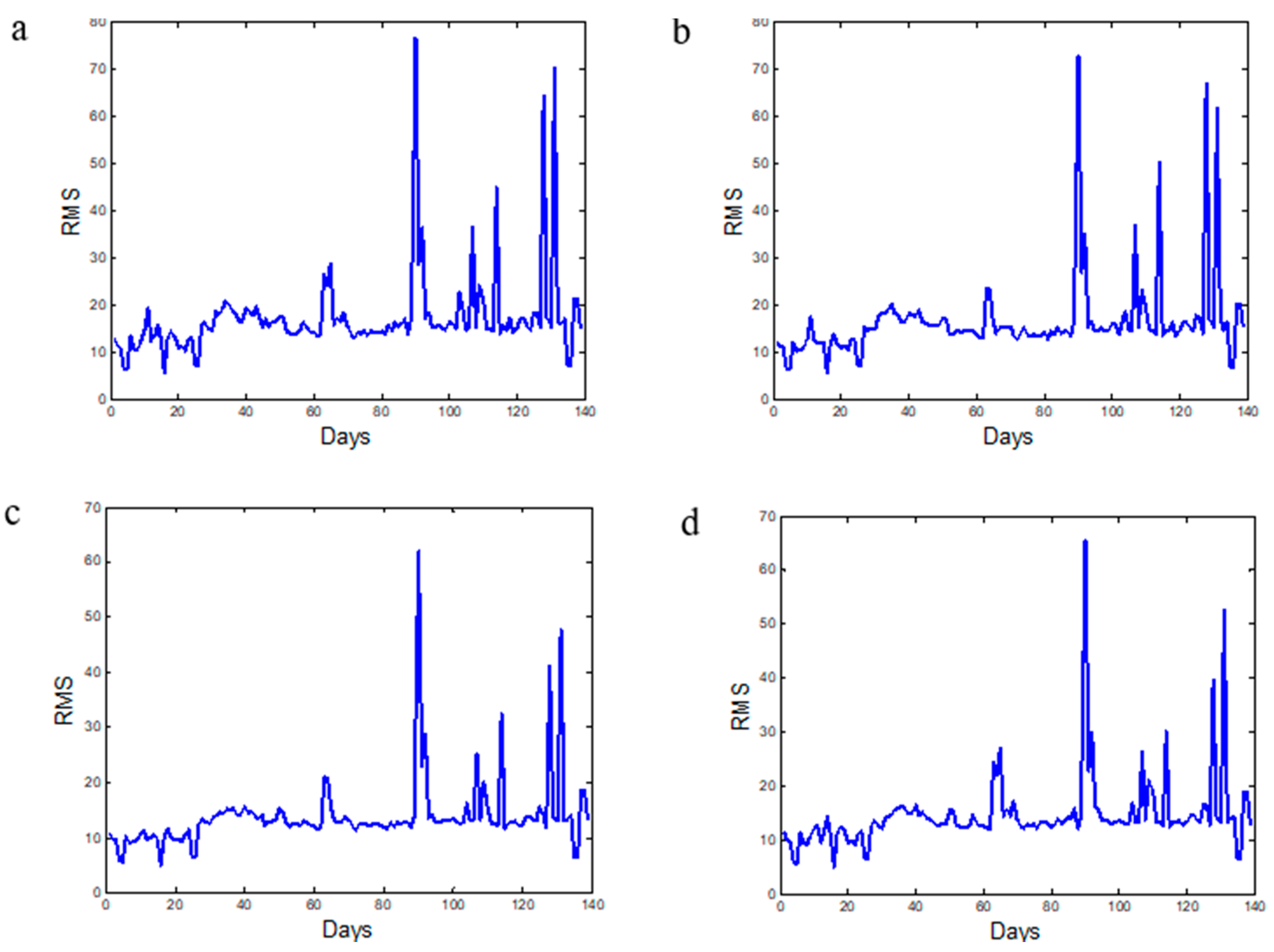
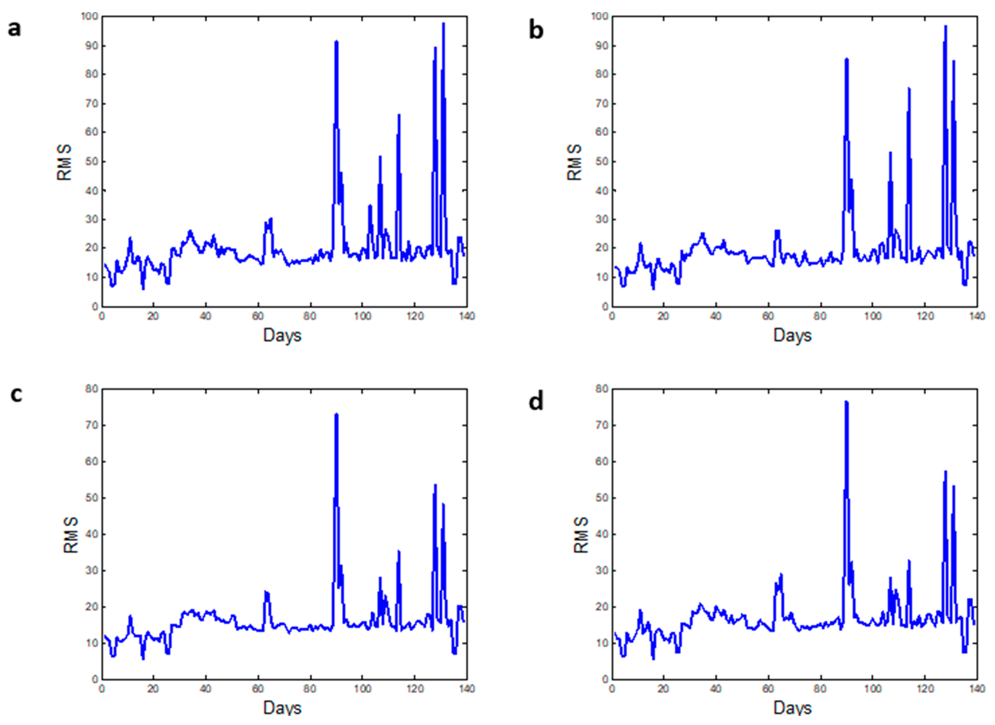
| RMS | The RMS value increase gradually as fault developed. However, RMS is unable to provide the information of incipient fault stage while it increases with the fault development [11]. | |
| Variance | Variance measures the dispersion of a signal around their reference mean value. | |
| Skewness | Skewness quantifies the asymmetry behavior of vibration signal through its probability density function (PDF). | |
| Kurtosis | Kurtosis quantifies the peak value of the PDF. The kurtosis value for normal rolling element bearing is well-recognized as 3. | |
| Shape factor | Shape factor is a value that is affected by an object’s shape but is independent of its dimensions [12]. | |
| Crest factor | Crest factor (CF) calculates how much impact occur during the rolling element and raceway contact. CF is appropriate for “spiky signals” [12]. | |
| Entropy | Entropy, , is a calculation of the uncertainty and randomness of a sampled vibration data. Given a set of probabilities, , the entropy can be calculated using the formulas as shown in the right column. | |
| Defect Mode | Fault Frequencies (Hz) (Calculation is Given in Appendix A) | |
|---|---|---|
| Axial | Radial | |
| Outer raceway (BPFO) | 1.32 | 0.55 |
| Inner raceway (BPFI) | 1.37 | 0.55 |
| Rolling element (BSF) | 0.43 | 0.54 |
| Vibration Data | IMFs of EMD (Hz) | ||||||||
|---|---|---|---|---|---|---|---|---|---|
| IMF2 | IMF3 | IMF4 | … | IMF11 | IMF12 | IMF13 | IMF14 | IMF15 | |
| 24 February | 641.81 | 694.52 | 390.35 | … | 2.47 | 1.44 | 0.69 | 0.33 | 1.99 |
| 3 May | 702.88 | 684.34 | 346.23 | … | 2.04 | 1.23 | 0.64 | 0.43 | 0.19 |
| 30 August | 651.72 | 679.86 | 245.92 | … | 1.37 | 0.68 | 0.33 | 0.10 | |
© 2017 by the authors. Licensee MDPI, Basel, Switzerland. This article is an open access article distributed under the terms and conditions of the Creative Commons Attribution (CC BY) license (http://creativecommons.org/licenses/by/4.0/).
Share and Cite
Caesarendra, W.; Tjahjowidodo, T. A Review of Feature Extraction Methods in Vibration-Based Condition Monitoring and Its Application for Degradation Trend Estimation of Low-Speed Slew Bearing. Machines 2017, 5, 21. https://doi.org/10.3390/machines5040021
Caesarendra W, Tjahjowidodo T. A Review of Feature Extraction Methods in Vibration-Based Condition Monitoring and Its Application for Degradation Trend Estimation of Low-Speed Slew Bearing. Machines. 2017; 5(4):21. https://doi.org/10.3390/machines5040021
Chicago/Turabian StyleCaesarendra, Wahyu, and Tegoeh Tjahjowidodo. 2017. "A Review of Feature Extraction Methods in Vibration-Based Condition Monitoring and Its Application for Degradation Trend Estimation of Low-Speed Slew Bearing" Machines 5, no. 4: 21. https://doi.org/10.3390/machines5040021