An Efficient Numerical Technique for the Nonlinear Fractional Kolmogorov–Petrovskii–Piskunov Equation


1
Department of Mathematics, Faculty of Science & Technology, Karnatak University, Dharwad 580003, India
2
Department of Mathematics, Faculty of Arts and Sciences, Cankaya University, Eskisehir Yolu 29. Km, Yukarıyurtcu Mahallesi Mimar Sinan Caddesi No, Etimesgut 406790, Turkey
3
Institute of Space Sciences, 077125 Magurele-Bucharest, Romania
*
Author to whom correspondence should be addressed.
Mathematics 2019, 7(3), 265; https://doi.org/10.3390/math7030265
Submission received: 20 December 2018
/
Revised: 7 March 2019
/
Accepted: 12 March 2019
/
Published: 14 March 2019
(This article belongs to the Special Issue Advances in Differential and Difference Equations with Applications 2019)
Abstract
:The -homotopy analysis transform method (-HATM) is employed to find the solution for the fractional Kolmogorov–Petrovskii–Piskunov (FKPP) equation in the present frame work. To ensure the applicability and efficiency of the proposed algorithm, we consider three distinct initial conditions with two of them having Jacobi elliptic functions. The numerical simulations have been conducted to verify that the proposed scheme is reliable and accurate. Moreover, the uniqueness and convergence analysis for the projected problem is also presented. The obtained results elucidate that the proposed technique is easy to implement and very effective to analyze the complex problems arising in science and technology.
1. Introduction
Integration and differentiation with arbitrary order is called fractional calculus (FC), and it is the general expansion of integer order calculus to arbitrary order. Derivatives of arbitrary order were invented by Leibnitz soon after the integer order derivatives. Recently, FC has become a powerful tool because of its favorable properties such as analyticity, linearity, and nonlocality. With the fast growth of digital computer knowledge, many researchers have started to work on the theory and applications of FC to present their view points.
Moreover, many pioneering references are available for diverse definitions of fractional calculus, this has laid the groundwork for FC study [1,2,3,4,5,6]. The theory of fractional-order calculus has been related to practical projects, and it has been applied to study many interesting topics including chaos theory [7], biomathematics [8], financial models [9], optics [10], and other areas. The analytical and numerical solutions for differential equations of fractional order present in the above phenomena play a vital role in describing the characters of nonlinear complex problems as they exist in daily life.
Fractional order models extend our concepts of differentiability, and they incorporate non-local and systematic memory effects through fractional order space and time derivatives [11]. These features allow us to model phenomena across multiple time and space scales without having to partition the problem into smaller and smaller compartments. The extent to which a fractional order model will span multiple scales is based on an underlying presumption that fractional derivatives can limit or capture salient features of complex phenomena. In interdisciplinary fields, many systems can be described more accurately and more conveniently by fractional differential equations. For instance, fractional derivatives have been widely used in mathematical modeling of viscoelastic materials [12]. The anomalous diffusion phenomena in nonhomogeneous media can be explained by non-integer, derivative-based equations of diffusion [13]. Another example of an element with fractional order is fractance, which is an electrical circuit with non-integer order impedance that has both resistance and capacitance properties [14]. Moreover, it has been shown that the dynamic process of heat conduction can be modeled more adequately via fractional order calculus [15]. In biology, the membranes of biological cells are proven to have fractional order electrical conductance and are classified among non-integer order systems [16,17]. In economics, it is known that some finance systems can display fractional order dynamics [18].
In [19], Kolmogorov, Petrovskii, and Piskunov initiated the traveling waves theory and derived an equation called Kolmogorov–Petrovskii–Piskunov (KPP) equation. The KPP equation initially arose from the study of genetic models in the increase of microorganisms. Later, it was applied to analyze various biological, physical, and chemical models. Mainly, it is used in biological models to elucidate the progression of microbiological population densities (cells or bacteria) in terms of space–time, as a result of diffusion mechanisms. Particularly, nonlocal models are designed to elucidate the patterns of formation in bacterial regions [20]. This helps to analyze the micro-morphogenesis, which is of particular interest in the elementary phenomena of contemporary microbiology [21]. Now, we consider a nonlinear KPP equation [22]:
where and are constants. The KPP equation contains various familiar nonlinear equations in mathematical physics. In the case of , and , it reduces to the Newll–Whitehead equation; For , and , it is called the FitzHugh–Nagumo equation; and for , and , it is a special case of the Fisher equation (i.e., ). In the present investigation, we consider the fractional KPP (FKPP) equation [23,24]:
with the initial condition . Here, specifies the state evolution over the spatial-temporal domain characterized by the coordinates , respectively.
Recently, a number of new and advanced schemes have been developed to study the differential systems of fractional orders. These schemes are in parallel to the formation of new computational algorithms and symbolic programming. Most of the complex phenomena, including chaos, solitons, asymptotic properties, singular formation, etc., remained undetected or were in feeble states in the pre-computer era. New mathematical theories and analytical techniques that have been combined with recent computational algorithms have precipitated this revolution in our understanding, and this aids us in our study of nonlinear phenomena.
A Chinese mathematician, Liao Shijun, proposed the homotopy analysis method (HAM) [25,26] by employing the fundamental concept of differential geometry and topology, called homotopy. Recently, HAM has been efficiently employed to analyze and find the solution for problems arising in distinct areas of science and technology. In connection with this, the q-homotopy analysis transform method (-HATM) was proposed by Singh et al. [27], which is an elegant amalgamation of -HAM and the Laplace transform. The future scheme controls and manipulates the series solution, which quickly converges to the exact solution in a short, permissible region. As a result, many authors have recently analyzed the different phenomena situated in different areas with the help of -HATM, including Srivastava et al. who studied models of vibration equations of arbitrary order [28], Singh et al. who were employed to find the solution to the fractional Drinfeld–Sokolov–Wilson equation [29], Bulut et al. who analyzed HIV infection of CD4+T lymphocyte cells with a fractional model [30], Kumar et al. who analyzed the model of Lienard’s equation [31], and many others [32,33,34,35].
On employing the methods with perturbation, linearization, or discretization techniques, we obtained only approximate solutions for nonlinear complex problems. These problems were appraised by exerting different schemes having their own limitations and weakness, including more time for evaluation, massive computational work, and obtaining divergent results. The classical technique (i.e., HAM) necessitates more time for computational work and a large computer memory. To overcome these limitations, there is a need to combine this technique with already available transform techniques. The enhancement of the proposed technique is its proficiency of amalgamating two strong algorithms to solve linear and nonlinear fractional differential equations, both numerically and analytically. The proposed method provides many strong properties, including nonlocal effect, a straightforward solution procedure, a large convergence region free from any assumptions, discretization, and perturbation. It is worth revealing that the Laplace transform with semi-analytical techniques requires less CPU time to evaluate solutions for nonlinear complex models and phenomena in science and technology. The -HATM solution involves two auxiliary parameters, and , which helps us to adjust and control the convergence of the solution. We can say that the proposed technique can decrease computation time and work compared to other traditional techniques while maintaining great efficiency of the obtained results. Therefore, in the present frame work we employ -HATM to investigate the nonlinear FKPP equation.
Analytical and numerical solutions for the nonlinear fractional differential equations are of fundamental importance since most complex phenomena are modelled mathematically by differential and integral equations, but actually require a fractional order. There are many methods available in the literature to solve these equations. The KPP equation is studied through distinct techniques like the discrimination algorithm [36], the (G’/G)-expansion method [37], the homotopy perturbation method (HMP) [23], the generalized two-dimensional differential transform method [24], and many others [22,38,39,40,41,42]. The rest of the paper is arranged as follows. In Section 2 the preliminaries of fractional order integrals and derivatives and the Laplace transform are presented. Section 3 concerns the fundamental procedure of the proposed algorithm for the fractional KPP equation. In Section 4 the convergence analysis of the technique is presented. In Section 5, a solution for the fractional KPP equation is investigated. In Section 6 and Section 7, the numerical simulation and discussions and concluding remarks are cited.
2. Preliminaries
We recall the definitions and notations of FC and the Laplace transform, which shall be employed in the present frame work:
Definition 1.
Definition 2.
The fractional derivative of in the Caputo [3] sense is defined as
3. Proposed Algorithm for the Fractional Kolmogorov–Petrovskii–Piskunov (KPP) Equation
In this segment, we applied a fundamental solution procedure of the proposed algorithm for the FKPP equitation. First, we consider a fractional order, nonlinear KPP equation:
subjected to the initial condition
where denotes the fractional Caputo derivative of the function Here, is a bounded function (i.e., for a number we have ), Now, by performing the on Equation (5) and make use of conditions provided in Equation (7), we get
We define the nonlinear operator with the assistance of Equation (8), as
where , and is a real function of and . For a non-zero auxiliary function, we construct a homotopy as follows [43]:
where is a symbol of , is an auxiliary parameter, is the embedding parameter, and is an initial guess of. The following results hold respectively for and:
Thus, by amplifying from to, the solution converges from to the solution. Expanding the function in series form by applying the Taylor theorem [44] near to, one can get
where
On choosing the auxiliary linear operator, and, the series (11) converges at and then it yields one of the solutions for Equation (6):
Now, the zero-th order deformation Equation (10) differentiates -times with respect to , is then divided by and finally assigns, which gives
where
Employing the inverse on Equation (15), it yields
Then, we define for the cited equation as follows:
where
By Equation (17), Equation (18) is reduced to
Finally, on solving Equation (20) we get the iterative terms of . The -HATM series solution is presented by
4. Convergence Analysis of the Technique
Here, we present the convergence analysis of the proposed algorithm for the FKPP equation
Theorem 1.
(Uniqueness theorem) The obtained solution for the FKPP Equation (6) with the aid of -HATM is unique wherever , where .
Proof.
The solution for the FKPP equation defined in Equation (6) is presented as
where
If possible, let and be the two distinct solutions for the FKKP equation such that and , then using the above relation, we have
By employing convolution theorem for LT, we obtained
where . By the help of the integral mean value, the above equation reduces to
Since , then, which gives . This proves the uniqueness of the solution. □
Theorem 2.
Proof.
Let be a Banach space of all continuous functions on with the norm symbolized as . First, we prove is a Cauchy sequence in the Banach space.
Now, consider
On employing a convolution theorem for LT, we get
With the aid of the integral mean value theorem [44,45], the above relation reduced to
Setting , it yields:
On using triangular inequality, we have
As , so , then we have
But , consequently as then , therefore, the sequence is a Cauchy sequence in . It yields and is a convergent sequence. This concludes our required results. □
5. Solution for the fractional KPP equation
In this part, we consider two distinct initial conditions for the FKPP equation to validate the applicability and efficiency of the proposed algorithms.
Case (i).
where is the Jacobi elliptic function, and and are arbitrary constants. The exact solution for the classical KPP equation is given by
On solving Equation (20) with the initial condition (24), we obtain
On continuing the same procedure, the remaining iterative terms can be found.
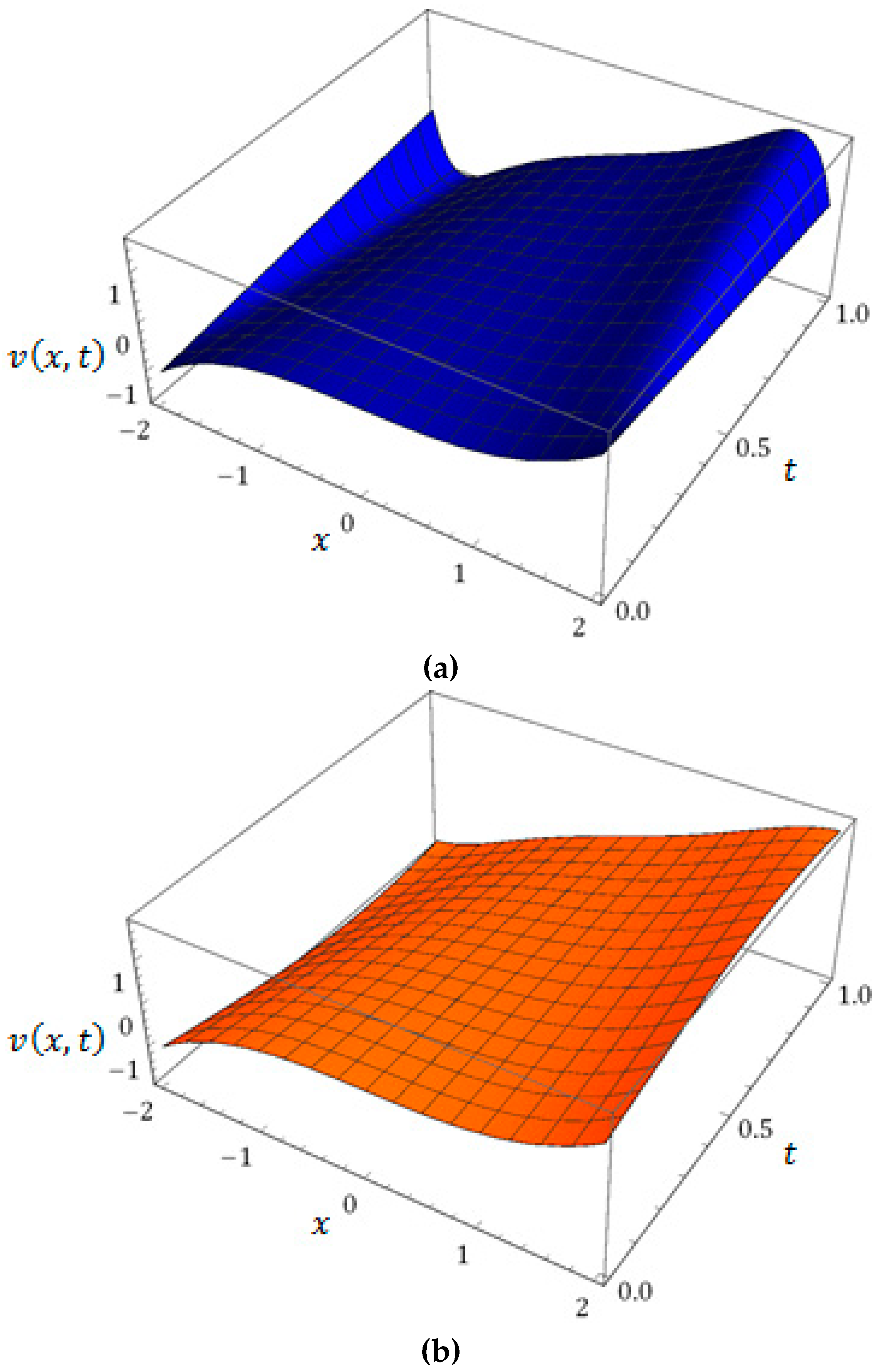
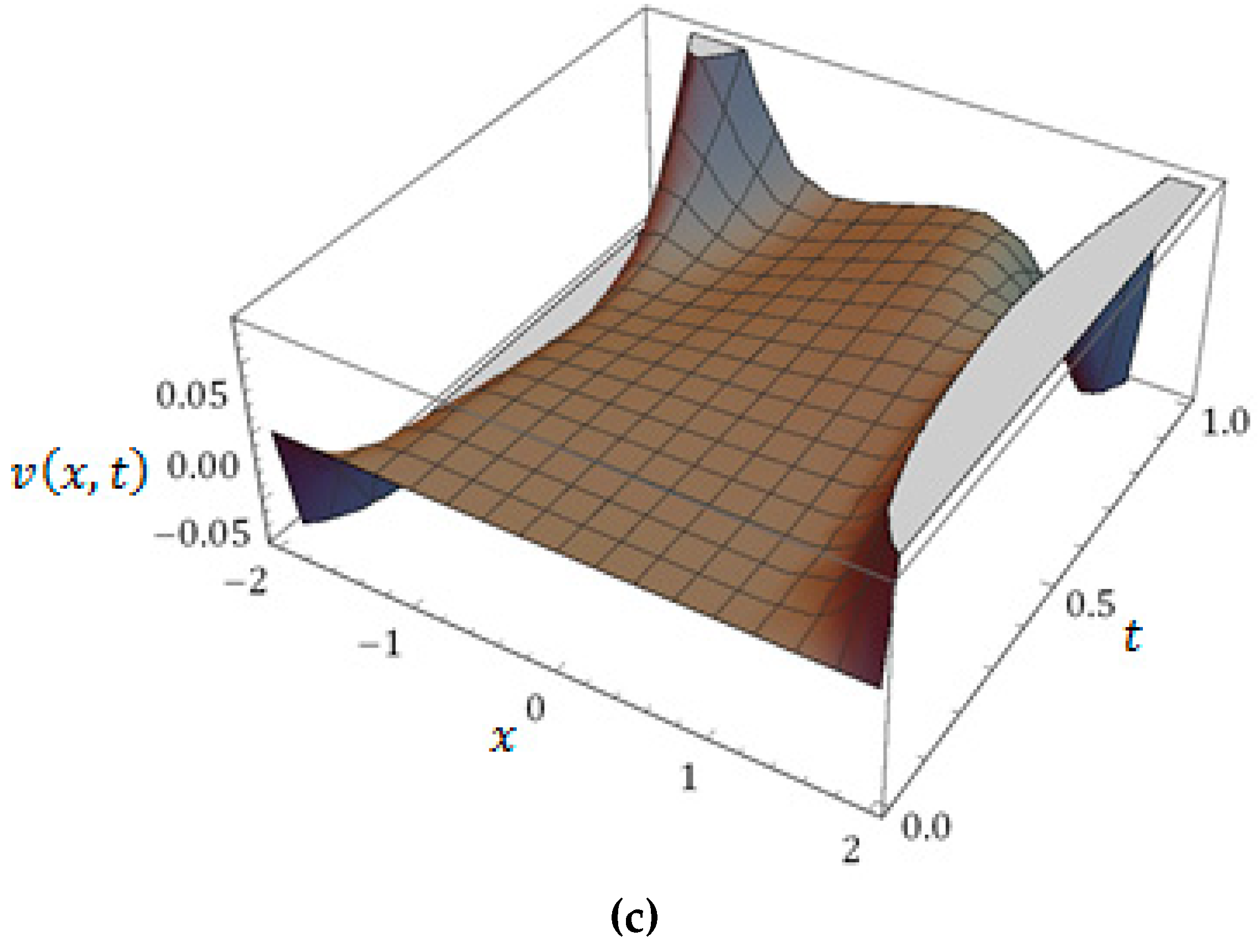
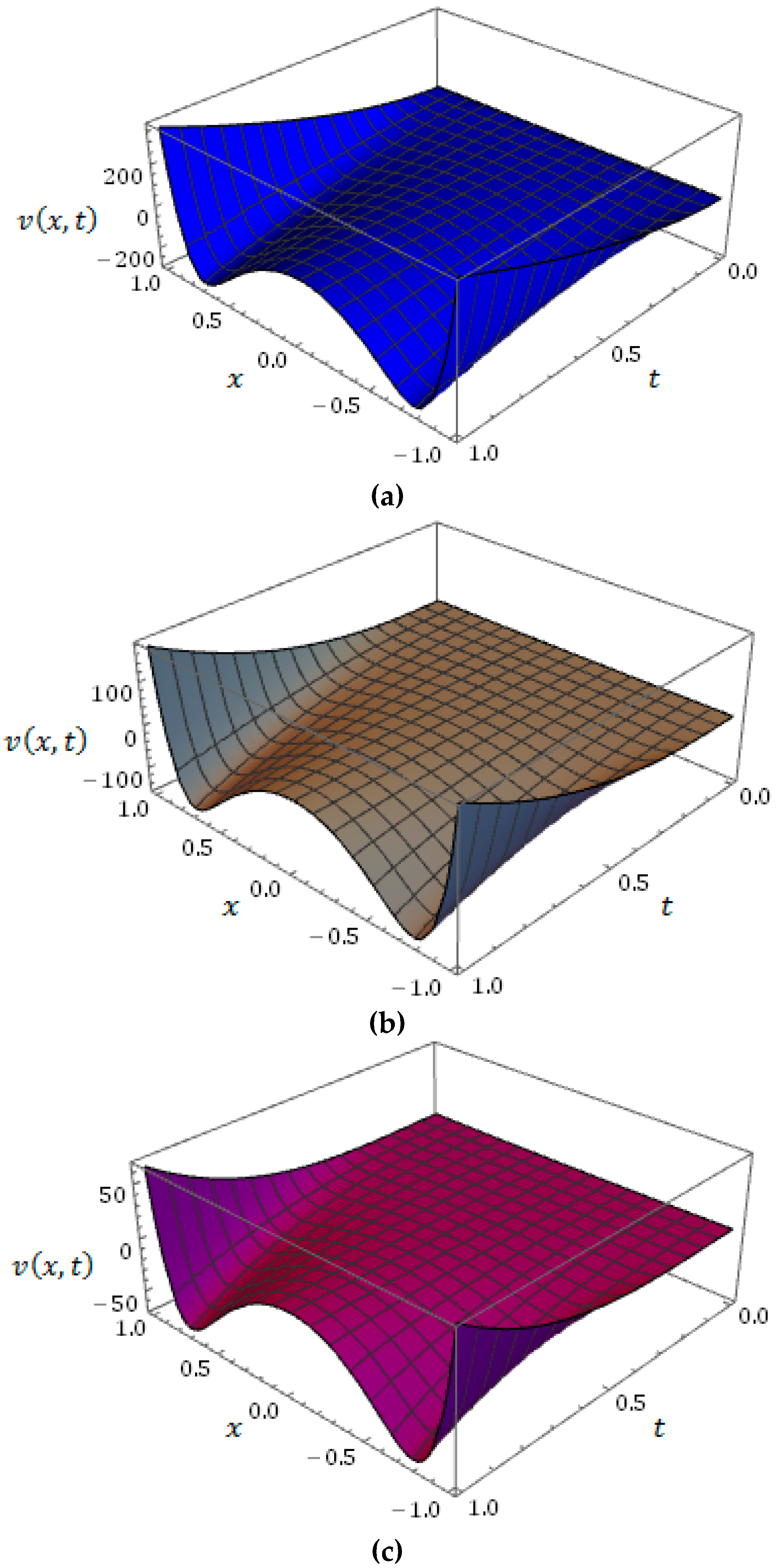
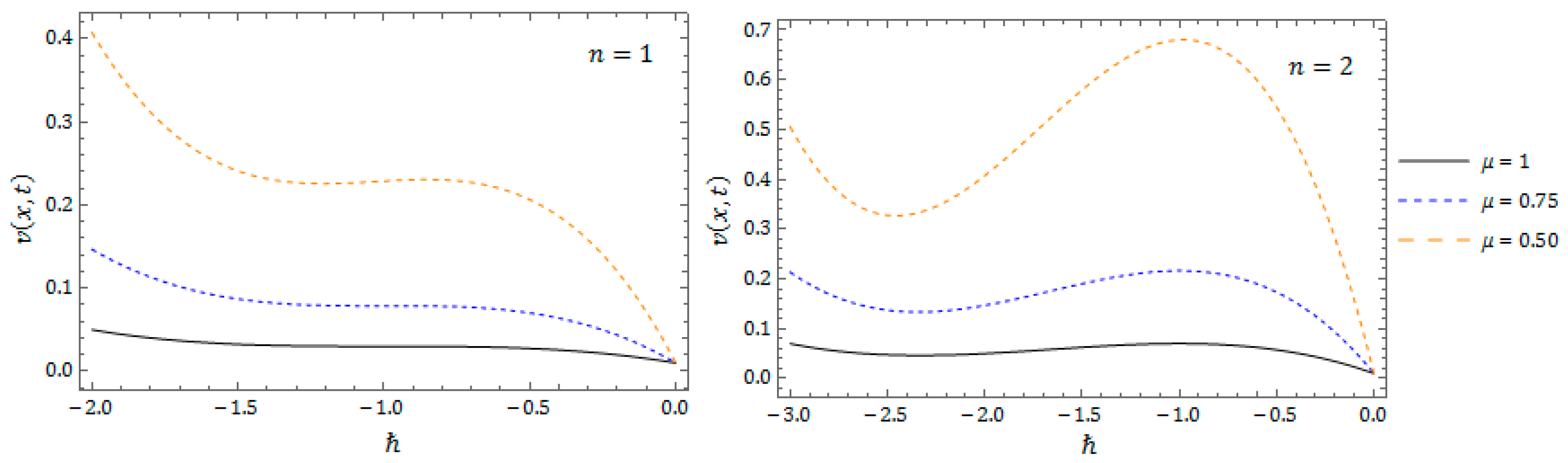
The nature of the solution obtained by -HATM for the FKPP equation with the initial conditions considered in Equation (25) is presented in Figure 1a, and the corresponding nature of the exact solution and surface of absolute error are presented in Figure 1b,c, respectively. Figure 2 is the responses of obtained solutions for case with distinct fractional Brownian motions and standard motions. Figure 3 represent the -curves with diverse values of and obtained by -HATM for case. This helps us to control and adjust the convergence region of the obtained solution.
The error analysis has been presented in order to show the efficiency of the proposed technique for the solution to the FKPP equation with the initial conditions considered in case , which is presented in Table 1, for diverse values of and with distinct fractional Brownian motions and standard motions. From the table we can see that as increases from to, the solution gets closer to the exact solution.
Case (ii).
On solving Equation (20) with the initial condition (25), we obtain
On continuing the same procedure, the remaining iterative terms can be found.
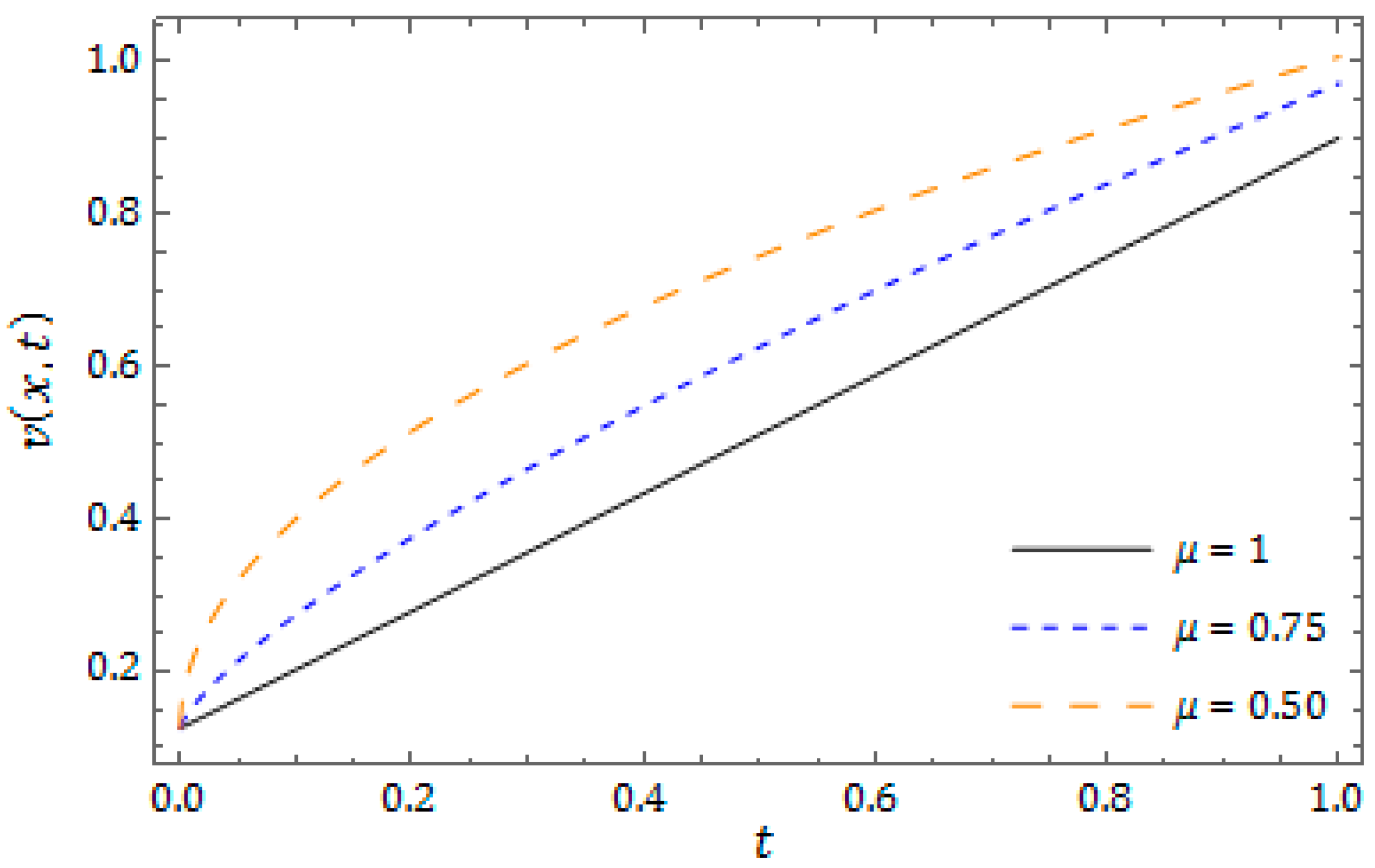
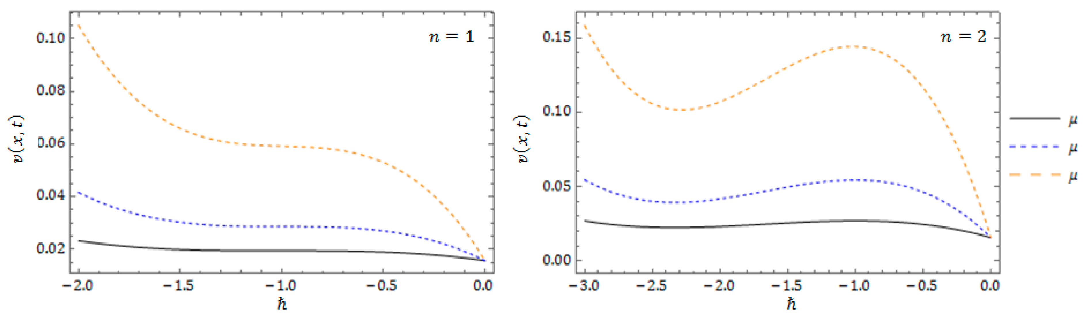
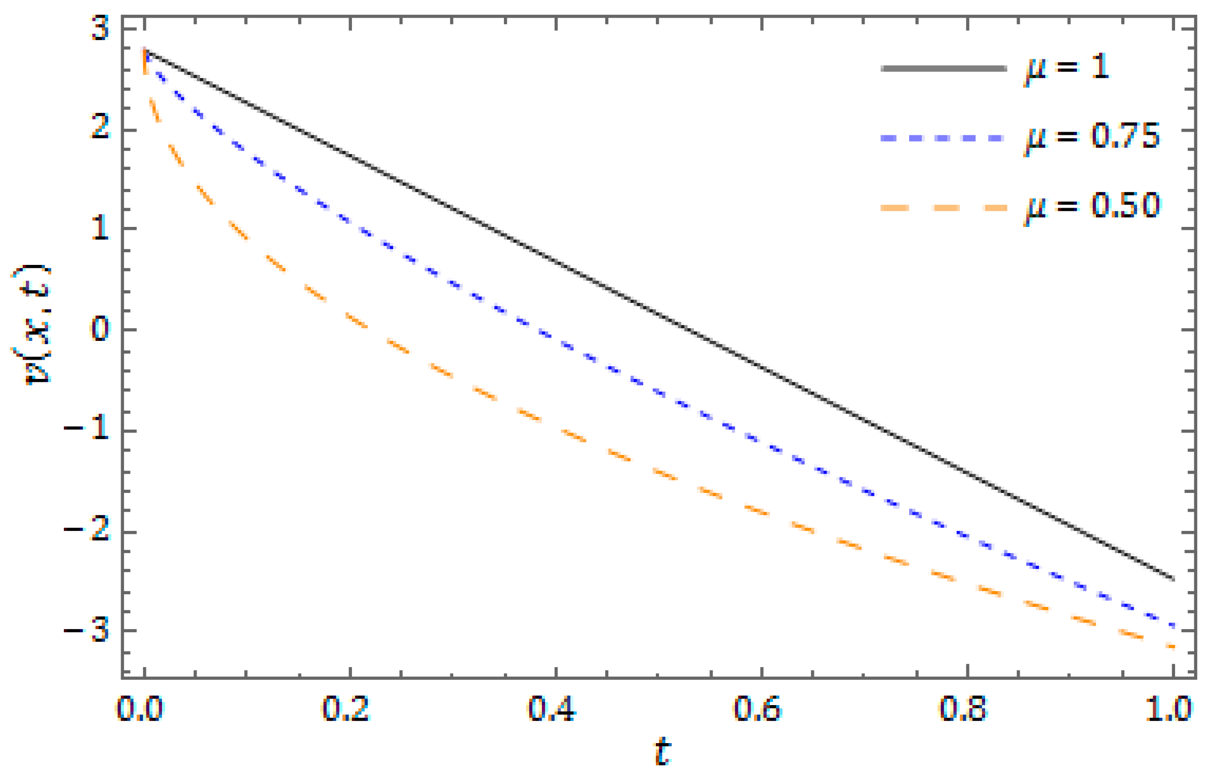
The nature of the FKPP equation with the initial conditions considered in Equation (26) for different (i.e., 0.50, 0.75, and 1) is observed in Figure 4, which elucidates the rule of fractional derivatives in the projected problem. Figure 5 represent the -curves with diverse values of and obtained by -HATM for case .
In order to show the efficiency of the proposed technique for case, the numerical simulations have been connected, which are presented in Table 2.
Case (iii).
where and are the Jacobi elliptic functions.
On solving Equation (20) with the initial condition (26), we obtain
On continuing the same procedure, the remaining iterative terms can be found. Then, the -HATM series solution for Equation (20) is presented by
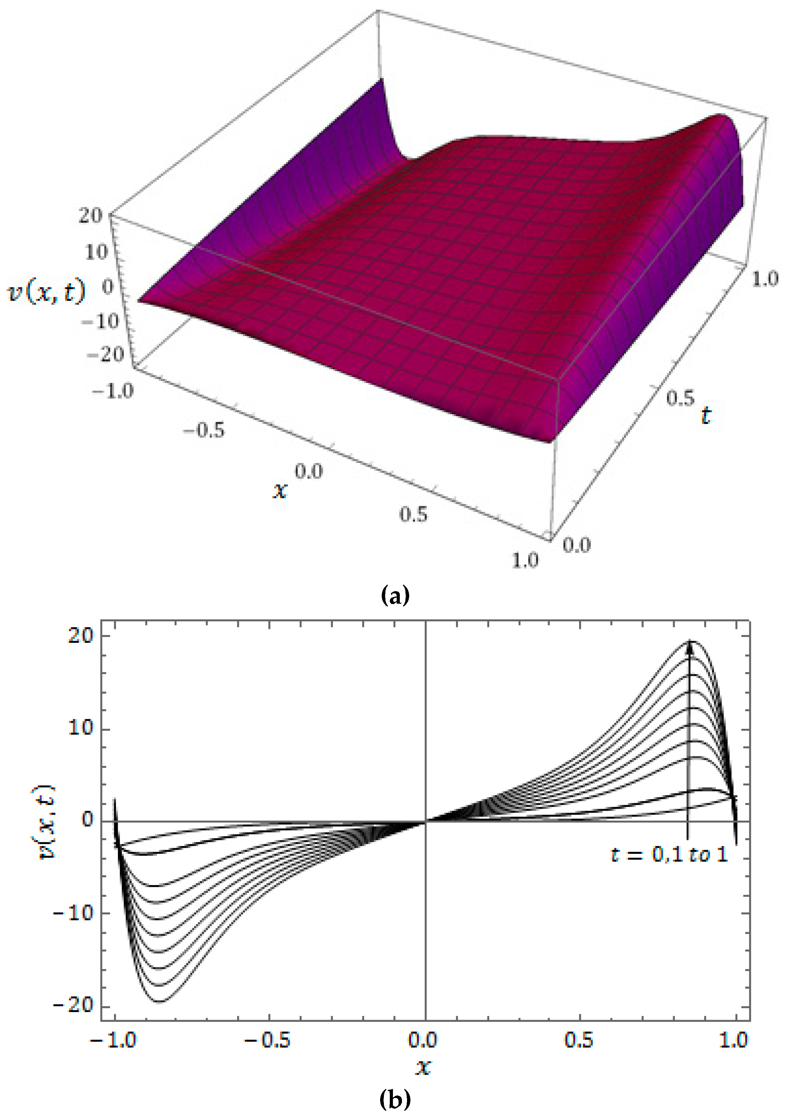
The surface of the considered equation with the initial conditions cited in Equation (27) is presented in Figure 6a, and the corresponding plot for diverse time is shown in Figure 6b. This helps us to understand the behavior of the KPP equation when spatial-temporal variables are changed. Figure 7 is the responses of obtained solutions for case with distinct fractional Brownian motions and standard motions. Figure 8 represent the -curves with distinct values of and obtained by -HATM for case. This aids us to control and adjust the convergence region of the obtained solution.
In order to show the efficiency of the proposed technique for case, the numerical simulations have been connected, which are presented in Table 3 for diverse values of and with distinct fractional Brownian motions and standard motions.
6. Numerical Results and Discussion
In this section, we conduct a numerical simulation for the obtained solution of the fractional order KPP equation with the help of -HATM. Further, the solution obtained by the proposed method is more accurate compared to the solution obtained by the other techniques. From the cited tables it is clear that the proposed problem noticeably depends on order. From the figures, we can see that as time increases, the solution to the FKPP equation also increases in both the cases.
We can see from the obtained solution that the solution procedure of the proposed method is straightforward and simple to implement, whereas the solution obtained with the help of techniques presented in [24] is difficult, and it requires more computation in order to evaluate more terms in the series solution. The proposed technique provides us two parameters, namely, auxiliary parameter and embedding parameter, which helps to control and adjust the convergence region of the obtained solution. From the tables and plots obtained in the present investigation, we can say that the proposed technique effectively captures the behavior of the FKPP equation. Moreover, the future method is very efficient to analyze the fractional order differential equations with initial conditions that have Jacobi elliptic functions with the help of the mathematical software MATHEMATICA (Version-10.4, Wolfram Research, Champaign, Illinois, US).
7. Conclusions
In this paper, we profitably employed -HATM to find the solution for the KPP equation of fractional order. We considered three cases with two distinct initial conditions having Jacobi elliptic functions, which were very difficult to solve with the aid perturbation, linearization, and discretization. The proposed algorithm was free from these difficulties. The novelty of the proposed technique is that it provides a nonlocal effect, a straightforward solution procedure, and a promising large convergence region. The convergence analysis is presented with the aid of Banach’s fixed point theory for the considered problem. In the present investigation we can see that the FKPP equation, having initial conditions analyzed with Jacobi elliptic functions, finds the approximated analytical solution in the series form. Further, the obtained solutions contain two parameters, which helps us to control the convergence of the obtained solution. Finally, we can conclude that the considered technique is highly coherent and it can be employed to examine wide classes of nonlinear mathematical models that have fractional orders. They can be applied for understanding the behaviors of complex phenomena in connected areas of science and technology.
Author Contributions
The authors declare that they carried out all the work in this manuscript, and read and approved the final manuscript.
Conflicts of Interest
The authors declare no conflict of interest.
References
- Liouville, J. Memoire sur quelques questions de geometrie et de mecanique, et sur un nouveau genre de calcul pour resoudre ces questions. J. Ecole Polytech. 1832, 13, 71–162. [Google Scholar]
- Riemann, G.F.B. Versuch Einer Allgemeinen Auffassung der Integration und Differentiation; Gesammelte Mathematische Werke: Leipzig, Germany, 1896. [Google Scholar]
- Caputo, M. Elasticita e Dissipazione; Zanichelli: Bologna, Italy, 1969. [Google Scholar]
- Miller, K.S.; Ross, B. An Introduction to Fractional Calculus and Fractional Differential Equations; A Wiley: New York, NY, USA, 1993. [Google Scholar]
- Podlubny, I. Fractional Differential Equations; Academic Press: New York, NY, USA, 1999. [Google Scholar]
- Kilbas, A.A.; Srivastava, H.M.; Trujillo, J.J. Theory and Applications of Fractional Differential Equations; Elsevier: Amsterdam, The Netherlands, 2006. [Google Scholar]
- Baleanu, D.; Wu, G.-C.; Zeng, S.-D. Chaos analysis and asymptotic stability of generalized Caputo fractional differential equations. Chaos Solitons Fractals 2017, 102, 99–105. [Google Scholar] [CrossRef]
- Baleanu, D.; Guvenc, Z.B.; Machado, J.A.T. New Trends in Nanotechnology and Fractional Calculus Applications; Springer: New York, NY, USA, 2010. [Google Scholar]
- Sweilam, N.H.; Hasan, M.M.A.; Baleanu, D. New studies for general fractional financial models of awareness and trial advertising decisions. Chaos Solitons Fractals 2017, 104, 772–784. [Google Scholar] [CrossRef]
- Esen, A.; Sulaiman, T.A.; Bulut, H.; Baskonus, H.M. Optical solitons and other solutions to the conformable space–time fractional Fokas–Lenells equation. Optik 2018, 167, 150–156. [Google Scholar] [CrossRef]
- Hilfer, R. Applications of Fractional Calculus in Physics; World Scientific: Singapore, 2000. [Google Scholar]
- Ogata, K. Modern Control Engineering; Prentice Hall: Upper Saddle River, NJ, USA, 2010. [Google Scholar]
- Arkhincheev, V.E. Anomalous diffusion in inhomogeneous media: Some exact results. Model. Meas. Control A 1993, 26, 11–29. [Google Scholar]
- Krishna, B.T. Studies on fractional order differentiators and integrators: A survey. Signal Process. 2011, 91, 386–426. [Google Scholar] [CrossRef]
- Djordjevic, V.D.; Atanackovic, T.M. Similarity solutions to nonlinear heat conduction and Burgers/Korteweg-deVries fractional equations. J. Comput. Appl. Math. 2008, 222, 701–714. [Google Scholar] [CrossRef]
- Cole, K.S. Electric Conductance of Biological Systems; Cold Spring Harbor: New York, NY, USA, 1993. [Google Scholar]
- Glockle, W.G.; Nonnenmacher, T.F. A fractional calculus approach to self-similar protein dynamics. Biophys. J. 1995, 68, 46–53. [Google Scholar] [CrossRef]
- Laskin, N. Fractional market dynamics. Phys. A 2000, 287, 482–492. [Google Scholar] [CrossRef]
- Kolmogorov, A.N.; Petrovskii, I.; Piskunov, N. A study of the diffusion equation with increase in the amount of substance and its application to a biology problem. Byul. Moskovskogo Gos. Univ. 1937, 1, 1–25. [Google Scholar]
- Fuentes, M.A.; Kuperman, M.N.; Kenkre, V.M. Nonlocal interaction effects on pattern formation in population dynamics. Phys. Rev. Lett. 2003, 91, 158104. [Google Scholar] [CrossRef] [PubMed]
- Murray, J.D. Mathematical Biology. I: An Introduction, 3rd ed.; Springer: New York, NY, USA, 2001. [Google Scholar]
- Unal, A.O. On the Kolmogorov-Petrovskii-Piskunov equation. Commun. Fac. Sci. Univ. Ank. Series A1 2013, 62, 1–10. [Google Scholar]
- Gepreel, K.A. The homotopy perturbation method applied to the nonlinear fractional Kolmogorov–Petrovskii–Piskunov equations. Appl. Math. Lett. 2011, 24, 1428–1434. [Google Scholar] [CrossRef]
- Song, L.-N.; Wang, W.-G. Approximate solutions of nonlinear fractional Kolmogorov-Petrovskii-Piskunov equations using an enhanced algorithm of the generalized two-dimensional differential transform method. Commun. Theor. Phys. 2012, 58, 182–188. [Google Scholar] [CrossRef]
- Liao, S.J. Homotopy analysis method and its applications in mathematics. J. Basic Sci. Eng. 1997, 5, 111–125. [Google Scholar]
- Liao, S.J. Homotopy analysis method: A new analytic method for nonlinear problems. Appl. Math. Mech. 1998, 19, 957–962. [Google Scholar]
- Singh, J.; Kumar, D.; Swroop, R. Numerical solution of time- and space-fractional coupled Burgers’ equations via homotopy algorithm. Alex. Eng. J. 2016, 55, 1753–1763. [Google Scholar] [CrossRef]
- Srivastava, H.M.; Kumar, D.; Singh, J. An efficient analytical technique for fractional model of vibration equation. Appl. Math. Model. 2017, 45, 192–204. [Google Scholar] [CrossRef]
- Singh, J.; Kumar, D.; Baleanu, D.; Rathore, S. An efficient numerical algorithm for the fractional Drinfeld–Sokolov–Wilson equation. Appl. Math. Comput. 2018, 335, 12–24. [Google Scholar] [CrossRef]
- Bulut, H.; Kumar, D.; Singh, J.; Swroop, R.; Baskonus, H.M. Analytic study for a fractional model of HIV infection of CD4+T lymphocyte cells. Math. Nat. Sci. 2018, 2, 33–43. [Google Scholar] [CrossRef]
- Kumar, D.; Agarwal, R.P.; Singh, J. A modified numerical scheme and convergence analysis for fractional model of Lienard’s equation. J. Comput. Appl. Math. 2018, 399, 405–413. [Google Scholar] [CrossRef]
- Veeresha, P.; Prakasha, D.G.; Baskonus, H.M. New numerical surfaces to the mathematical model of cancer chemotherapy effect in Caputo fractional derivatives. Chaos 2019, 29, 013119. [Google Scholar] [CrossRef] [PubMed]
- Veeresha, P.; Prakasha, D.G.; Magesh, N.; Nandeppanavar, M.M.; Christopher, A.J. Numerical simulation for fractional Jaulent-Miodek equation associated with energy-dependent Schrodinger potential using two novel techniques. arXiv, 2019; arXiv:1810.06311. [Google Scholar]
- Prakash, A.; Veeresha, P.; Prakasha, D.G.; Goyal, M. A homotopy technique for fractional order multi-dimensional telegraph equation via Laplace transform. Eur. Phys. J. Plus 2019, 134, 1–18. [Google Scholar] [CrossRef]
- Veeresha, P.; Prakasha, D.G.; Baskonus, H.M. Novel simulations to the time-fractional Fisher’s equation. Math. Sci. 2019, 1–10. [Google Scholar] [CrossRef]
- Wang, D.S.; Li, H.B. Single and multi-solitary wave solutions to a class of nonlinear evolution equations. J. Math. Anal. Appl. 2008, 343, 273–298. [Google Scholar] [CrossRef]
- Feng, J.S.; Li, W.J.; Wan, Q.L. Using (G’/G)-expansion method to seek the traveling wave solution of Kolmogorov-Petrovskii-Piskunov equation. Appl. Math. Comput. 2011, 217, 5860–5865. [Google Scholar]
- Hariharan, G. The homotopy analysis method applied to the Kolmogorov-Petrovskii-Piskunov (KPP) and fractional KPP equations. J. Math. Chem. 2013, 51, 992–1000. [Google Scholar] [CrossRef]
- Nikitin, A.G.; Barannyk, T.A. Solitary waves and other solutions for nonlinear heat equations. Cent. Eur. J. Math. 2005, 2, 840–858. [Google Scholar] [CrossRef]
- Ma, W.X.; Fuchssteiner, B. Explicit and exact solutions to a Kolmogorov-Petrovskii-Piskunov equation. Int. J. Non-Linear Mech. 1996, 31, 329–338. [Google Scholar] [CrossRef]
- Qin, C.-Y.; Tian, S.-F.; Wang, X.-B.; Zou, L.; Zhang, T.-T. Lie symmetry analysis, conservation laws and analytic solutions of the time fractional Kolmogorov–Petrovskii–Piskunov equation. Chin. J. Phys. 2018, 56, 1734–1742. [Google Scholar] [CrossRef]
- Zayed, E.M.; Alurrf, K.A.; Nowehy, A.G.A. Many Exact Solutions of the Nonlinear KPP Equation Using the Bäcklund Transformation of the Riccati Equation. Int. J. Opt. Photonic Eng. 2017, 2, 1–7. [Google Scholar]
- Prakasha, D.G.; Veeresha, P.; Rawashdeh, M.S. Numerical solution for (2+1)-dimensional time-fractional coupled Burger equations using fractional natural decomposition method. Math. Meth. Appl. Sci. 2019, 42, 1–19. [Google Scholar] [CrossRef]
- Odibat, Z.M.; Shawagfeh, N.T. Generalized Taylor’s formula. Appl. Math. Comput. 2007, 186, 286–293. [Google Scholar]
- Argyros, I.K. Convergence and Applications of Newton-Type Iterations; Springer Science & Business Media: Berlin, Germany, 2008. [Google Scholar]
- Magrenan, A.A. A new tool to study real dynamics: The convergence plane. Appl. Math. Comput. 2014, 248, 215–224. [Google Scholar] [CrossRef]
Figure 1.
(a) Response of the q-homotopy analysis transform method (-HATM) solution. (b) Nature of Exact solution. (c) Surface of Absolute error for case at , and .
Figure 1.
(a) Response of the q-homotopy analysis transform method (-HATM) solution. (b) Nature of Exact solution. (c) Surface of Absolute error for case at , and .


Figure 2.
Nature of the -HATM solution in case with respect to at , and for diverse .

Figure 3.
-curves obtained for in case with diverse when , and at distinct.

Figure 4.
Surface of -HATM solution for case at (a) ; (b) ; and (c) when and .

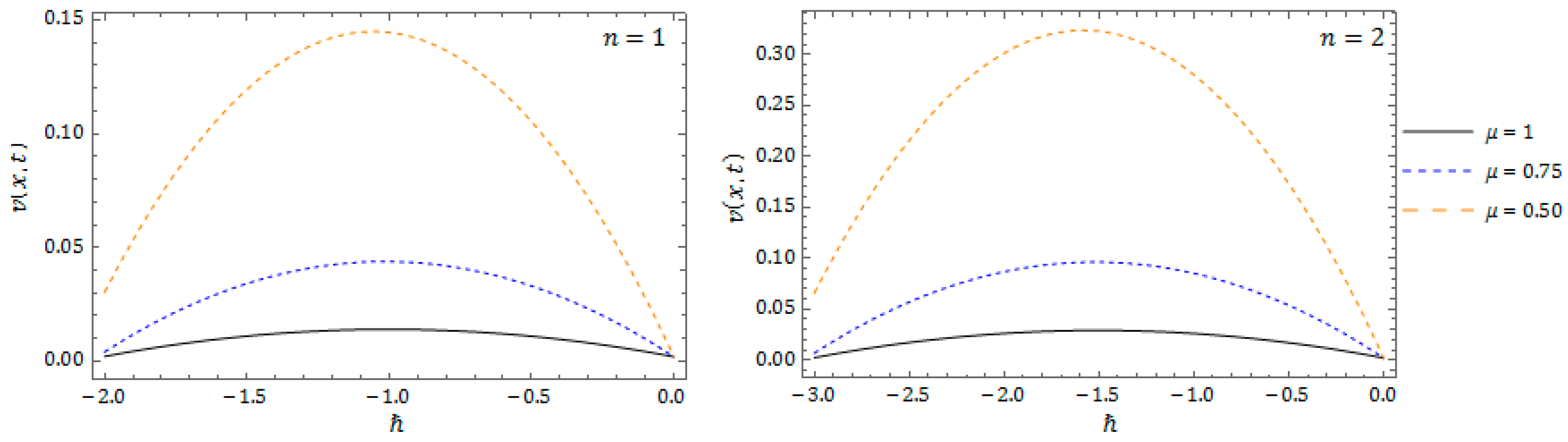
Figure 5.
-curves obtained for in case with diverse when and at distinct.

Figure 6.
(a) Surface of -HATM solution. (b) Nature of obtained solution at different times is from for case at , and.
Figure 6.
(a) Surface of -HATM solution. (b) Nature of obtained solution at different times is from for case at , and.

Figure 7.
Response of -HATM solution in case with respect to at , and for diverse .

Figure 8.
-curves obtained for in case with diverse when and at distinct.


Table 1.
Numerical simulations for fractional Kolmogorov–Petrovskii–Piskunov (FKPP) equation in terms of absolute error considered in case using -HATM at , and with distinct and for different.
Table 1.
Numerical simulations for fractional Kolmogorov–Petrovskii–Piskunov (FKPP) equation in terms of absolute error considered in case using -HATM at , and with distinct and for different.
| x | t | |||
|---|---|---|---|---|
| 0.2 | 0.02 | 0.004048 | 0.001614 | |
| 0.04 | 0.006276 | 0.002612 | ||
| 0.06 | 0.007984 | 0.003405 | ||
| 0.08 | 0.009382 | 0.004070 | ||
| 0.1 | 0.010561 | 0.004641 | ||
| 0.4 | 0.02 | 0.008131 | 0.003243 | |
| 0.04 | 0.012647 | 0.005266 | ||
| 0.06 | 0.016140 | 0.006892 | ||
| 0.08 | 0.019029 | 0.008272 | ||
| 0.1 | 0.021493 | 0.009474 | ||
| 0.6 | 0.02 | 0.012305 | 0.004914 | |
| 0.04 | 0.019220 | 0.0080222 | ||
| 0.06 | 0.024642 | 0.010555 | ||
| 0.08 | 0.029180 | 0.012738 | ||
| 0.1 | 0.033108 | 0.014673 | ||
| 0.8 | 0.02 | 0.016605 | 0.006656 | |
| 0.04 | 0.026002 | 0.010896 | ||
| 0.06 | 0.033399 | 0.014373 | ||
| 0.08 | 0.039628 | 0.017386 | ||
| 0.1 | 0.045047 | 0.020072 | ||
| 1 | 0.02 | 0.020854 | 0.008402 | |
| 0.04 | 0.032340 | 0.013606 | ||
| 0.06 | 0.041138 | 0.017723 | ||
| 0.08 | 0.048301 | 0.021142 | ||
| 0.1 | 0.054307 | 0.024043 |
Table 2.
Numerical simulations for the equation considered in case using -HATM at and with distinct and for different.
Table 2.
Numerical simulations for the equation considered in case using -HATM at and with distinct and for different.
| x | t | μ = 0.7 | μ = 0.8 | μ = 0.9 | μ = 1 |
|---|---|---|---|---|---|
| 0.01 | 0.2 | 0.71354 | 0.59265 | 0.48863 | 0.40010 |
| 0.4 | 1.15909 | 1.03179 | 0.91172 | 0.80012 | |
| 0.6 | 1.53948 | 1.42709 | 1.31320 | 1.20010 | |
| 0.8 | 1.88289 | 1.79638 | 1.70125 | 1.60010 | |
| 1 | 2.20119 | 2.14744 | 2.07961 | 2.00011 | |
| 0.05 | 0.2 | 0.71591 | 0.59502 | 0.49101 | 0.40249 |
| 0.4 | 1.16139 | 1.03412 | 0.91407 | 0.80246 | |
| 0.6 | 1.54170 | 1.42936 | 1.31549 | 1.20242 | |
| 0.8 | 1.88502 | 1.79856 | 1.70347 | 1.60236 | |
| 1 | 2.20323 | 2.14953 | 2.08174 | 2.00227 | |
| 0.1 | 0.2 | 0.72283 | 0.60217 | 0.49829 | 0.40986 |
| 0.4 | 1.16738 | 1.04053 | 0.92080 | 0.80942 | |
| 0.6 | 1.54654 | 1.43477 | 1.32138 | 1.20870 | |
| 0.8 | 1.88855 | 1.80275 | 1.70827 | 1.60769 | |
| 1 | 2.20530 | 2.15230 | 2.08521 | 2.00640 |
Table 3.
Numerical simulations for the equation considered in case using . -HATM at and with distinct and for different.
Table 3.
Numerical simulations for the equation considered in case using . -HATM at and with distinct and for different.
| x | t | μ = 0.8 | μ = 0.9 | μ = 1 |
|---|---|---|---|---|
| 0.1 | 0.02 | 0.39544 | 0.31857 | 0.25627 |
| 0.04 | 0.73580 | 0.63051 | 0.53892 | |
| 0.06 | 1.07771 | 0.95890 | 0.84998 | |
| 0.08 | 1.42750 | 1.30632 | 1.18942 | |
| 0.1 | 1.78728 | 1.67345 | 1.55725 | |
| 0.2 | 0.02 | 1.03187 | 0.79132 | 0.61147 |
| 0.04 | 2.17367 | 1.76387 | 1.43330 | |
| 0.06 | 3.48467 | 2.94515 | 2.48151 | |
| 0.08 | 4.95178 | 4.32609 | 3.75607 | |
| 0.1 | 6.56361 | 5.89892 | 5.25702 | |
| 0.3 | 0.02 | 2.14834 | 1.57388 | 1.16766 |
| 0.04 | 4.99339 | 3.89101 | 3.03371 | |
| 0.06 | 8.49589 | 6.94886 | 5.65234 | |
| 0.08 | 12.5737 | 10.6995 | 9.02354 | |
| 0.1 | 17.1721 | 15.1092 | 13.1473 | |
| 0.4 | 0.02 | 3.92819 | 2.79270 | 2.01364 |
| 0.04 | 9.67310 | 7.36715 | 5.60298 | |
| 0.06 | 16.9775 | 13.6543 | 10.8974 | |
| 0.08 | 25.6269 | 21.5326 | 17.8969 | |
| 0.1 | 35.4848 | 30.9193 | 26.6014 | |
| 0.5 | 0.02 | 6.27845 | 4.41081 | 3.14532 |
| 0.04 | 15.8083 | 11.9311 | 8.98311 | |
| 0.06 | 28.0760 | 22.4336 | 17.7701 | |
| 0.08 | 42.6940 | 35.7006 | 29.5059 | |
| 0.1 | 59.4191 | 51.5854 | 44.1909 |
© 2019 by the authors. Licensee MDPI, Basel, Switzerland. This article is an open access article distributed under the terms and conditions of the Creative Commons Attribution (CC BY) license (http://creativecommons.org/licenses/by/4.0/).
Share and Cite
MDPI and ACS Style
Veeresha, P.; Prakasha, D.G.; Baleanu, D. An Efficient Numerical Technique for the Nonlinear Fractional Kolmogorov–Petrovskii–Piskunov Equation. Mathematics 2019, 7, 265. https://doi.org/10.3390/math7030265
AMA Style
Veeresha P, Prakasha DG, Baleanu D. An Efficient Numerical Technique for the Nonlinear Fractional Kolmogorov–Petrovskii–Piskunov Equation. Mathematics. 2019; 7(3):265. https://doi.org/10.3390/math7030265
Chicago/Turabian StyleVeeresha, Pundikala, Doddabhadrappla Gowda Prakasha, and Dumitru Baleanu. 2019. "An Efficient Numerical Technique for the Nonlinear Fractional Kolmogorov–Petrovskii–Piskunov Equation" Mathematics 7, no. 3: 265. https://doi.org/10.3390/math7030265
Note that from the first issue of 2016, this journal uses article numbers instead of page numbers. See further details here.