Back to Basics: Meaning of the Parameters of Fractional Order PID Controllers
by
 , , , and
Inés Tejado
1,* ,
,
Blas M. Vinagre
1 ,
,
José Emilio Traver
1,
Javier Prieto-Arranz
1,2 and
Cristina Nuevo-Gallardo
1 1
Industrial Engineering School, University of Extremadura, 06006 Badajoz, Spain
2
School of Industrial Engineering, University of Castilla-La Mancha, 13071 Ciudad Real, Spain
*
Author to whom correspondence should be addressed.
Mathematics 2019, 7(6), 530; https://doi.org/10.3390/math7060530
Submission received: 8 May 2019
/
Revised: 1 June 2019
/
Accepted: 4 June 2019
/
Published: 11 June 2019
(This article belongs to the Special Issue Fractional Order Systems)
Abstract
:The beauty of the proportional-integral-derivative (PID) algorithm for feedback control is its simplicity and efficiency. Those are the main reasons why PID controller is the most common form of feedback. PID combines the three natural ways of taking into account the error: the actual (proportional), the accumulated (integral), and the predicted (derivative) values; the three gains depend on the magnitude of the error, the time required to eliminate the accumulated error, and the prediction horizon of the error. This paper explores the new meaning of integral and derivative actions, and gains, derived by the consideration of non-integer integration and differentiation orders, i.e., for fractional order PID controllers. The integral term responds with selective memory to the error because of its non-integer order , and corresponds to the area of the projection of the error curve onto a plane (it is not the classical area under the error curve). Moreover, for a fractional proportional-integral (PI) controller scheme with automatic reset, both the velocity and the shape of reset can be modified with . For its part, the derivative action refers to the predicted future values of the error, but based on different prediction horizons (actually, linear and non-linear extrapolations) depending on the value of the differentiation order, . Likewise, in case of a proportional-derivative (PD) structure with a noise filter, the value of allows different filtering effects on the error signal to be attained. Similarities and differences between classical and fractional PIDs, as well as illustrative control examples, are given for a best understanding of new possibilities of control with the latter. Examples are given for illustration purposes.
1. Introduction
The proportional-integral-derivative (PID) controller is distinguished as the most common form of feedback. In process control today, more than 95% of the control loops are of PID type, but these controllers can be found in all areas where control is used.
Despite its straightforward structure, the popularity of PID controllers lies in the simplicity of the design procedures and in the effectiveness obtained to the system performance [1]. Those are the main reasons why PID controllers have survived many changes in technology, from mechanics and pneumatics to microprocessors via electronic tubes, transistors, integrated circuits, among others. Actually, practically all PID controllers made today are based on microprocessors, so this electronic element has had a dramatic influence on this kind of control providing PIDs additional advances features, such as gain scheduling, continuous adaptation, and automatic tuning [2].
From the control engineering point of view, improving system behavior is the major concern. To that end, the generalization of classical PID controllers to non-integer orders of integration and differentiation was firstly proposed in [3]. Intuitively, with this extension of classical PIDs there are more tuning parameters and, consequently, more flexibilities in adjusting time and frequency responses of the control system. This also translates in more robustness in designs.
However, the first step when applying an existing or new controller is to understand exactly what their actions can do in closed-loop in order to take full advantage of the possible effects on the system response. In the case of integer order, the interpretation of the three actions of PIDs seems to be clear [4,5,6]:
- the proportional action is simply proportional to the current control error;
- the integral action is related to the past values of the control error, so represents the accumulated error, i.e., the area under the error curve;
- the derivative action predicts future values of the error or, in other words, corrects based on the rate of change of the deviation from the set-point.
Since the pioneering work of Podlubny, there is ample evidence that supports that fractional order PIDs (FOPIDs) have been extensively studied and applied in many fields. Undoubtedly, the lists that are reported below are quite far from aiming at completeness, failing to mention literal hundreds of other published texts related to FOPIDs; relevant and recent papers were selected for giving the reader an idea of the development volume on this topic that can be found in the specialized literature. Fundamentals of FOPIDs can be found in, e.g., [7,8,9,10]. In what concerns design methods, among the reported, the following can be highlighted: Ziegler–Nichols-type rules [11,12,13,14], optimal tuning [15,16,17,18], tuning for robustness purposes [19,20,21], auto-tuning [22,23], and tuning based on reducing the number of parameters [24]. Likewise, numerous advanced control schemes based on FOPID controllers were proposed, such as, Smith predictors structures [25,26,27], internal mode control [28,29,30], hybrid control [31], gain scheduling [32,33,34], gain and order scheduling [35,36], among others. Current reviews in the development of FOPIDs can be found in [37,38,39,40,41,42]; likewise, few current examples of application in industry are described in [43,44,45,46,47,48,49,50].
Despite so many variations and applications of the FOPID algorithm, as well as design and tuning methods, up to now a detailed description of the meaning of the parameters of such controllers cannot be found in the literature. Nevertheless, although few, studies on the geometric and physical interpretation of integrals and derivatives of arbitrary (not necessary integer) order have been published [51,52], but it still remains as an open problem.
These circumstances make the understanding of the meaning of the parameters of FOPIDs a priority. With so much in play, this paper explores the new meaning of integral and derivative actions, and gains, derived by the consideration of non-integer integration and differentiation orders. Similarities and differences between classical and fractional PIDs, as well as illustrative control examples, are given for a best understanding of new possibilities of control with the latter.
The remainder of this paper is organized as follows. Section 2 describes the control algorithm of classical PID and its generalization to non-integer order. Section 3 explains the meaning of the parameters of non-integer PIDs. Section 4 discusses similarities and differences between classical and fractional PIDs. Illustrative examples are given in Section 5. Main conclusions of this paper are drawn in Section 6.
2. Generalities
This section describes the control algorithm of classical PIDs and its generalization to non-integer order.
2.1. Classical PID Controller
The use of PID control consists of applying properly the combination of three types of corrective actions to the error signal, which represents how far or near is the desired output from the actual output. As widely known, these three control actions are proportional, integral and derivative.
The key aspect when tuning PID controllers is in deciding how to best combine those three terms to achieve the most efficient regulation of the process variable for the considered problem. As well known, the most obvious way is to use a simple weighted sum where each term is multiplied by a tuning constant or gain, and the results are then added together as follows:
where is the control signal, is the control error (, i.e., the difference between the desired set-point, , and the measured process variable, y), and , , and are the controller parameters: proportional gain, integral time constant, and derivative time constant, respectively.
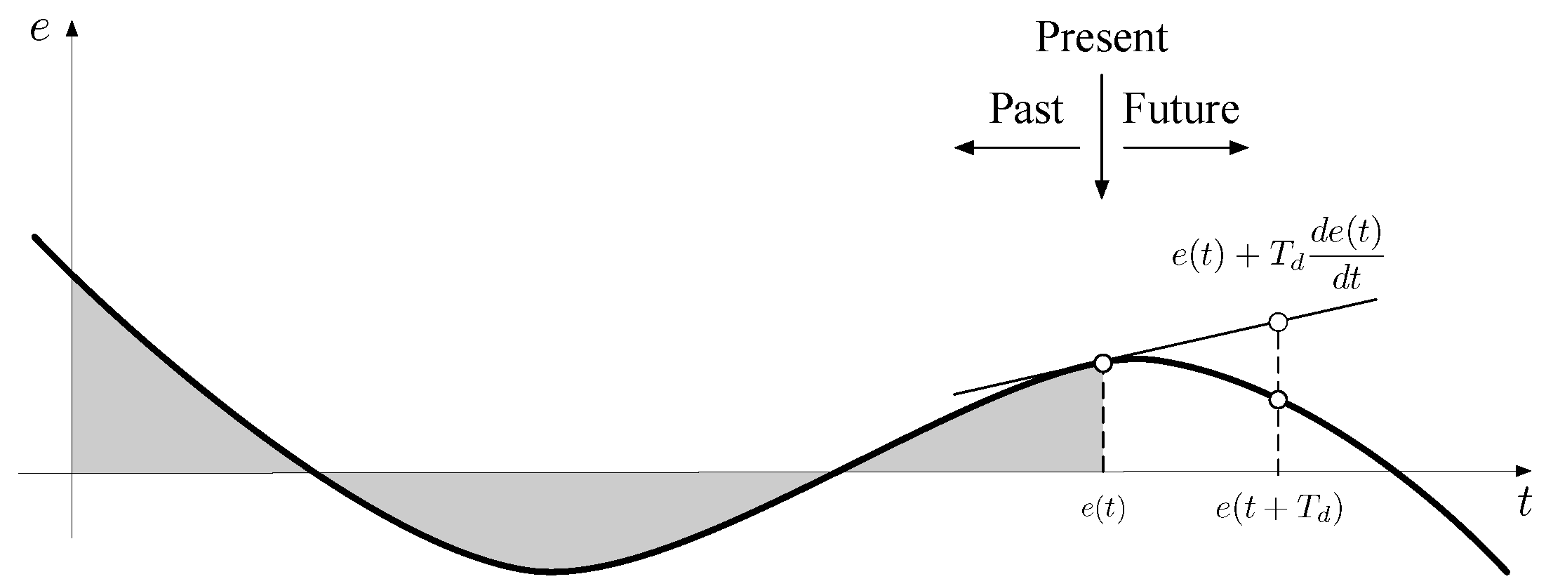
Control law (1) guarantees that the present (due to the proportional action), the past (by means of the integral action) and the future of the error (by the derivative action) are taken into account, as shown in Figure 1. Two main observations can be made to (1): (1) the controller needs only compute the current error between the measured process variable and the desired set-point to calculate how much and how fast that difference has been changing over time, and (2) the relative contributions of each term then can be then adjusted by choosing appropriate values of the controller parameters.
2.2. Fractional Order PID Controller
The generalization to non-integer orders of (1) leads to the typical algorithm of a FOPID controller, i.e.,
where and are the non-integer orders of the integral and derivative terms, respectively, and is the fractional operator defined as Riemann–Liouville as [10,53]
(n is a general non-integer order, and , the gamma function).
Similarly to the classical version, control law (2) combines the three natural ways of taking into account the error: current, accumulated, and predicted error. However, in contrast to the integer counterpart, fractional operators are non local, which results in new meaning of the integral and derivative actions, and gains. In particular, the fractional integration of the error is not already the area under its curve; it can be viewed as the area of the projection of the curve onto a plane. Hence, what the integration order is doing is a selection of the history of the error or, what is the same, the integral term responds with selective memory to the past values of the error. For its part, the action of a controller with proportional and fractional derivative action may be interpreted as if the control is made proportional to the predicted process output, where the prediction is definitively different from the classical case: it is made by extrapolating the error by a straight line that is not tangent to the error curve at the current value of the error, or by a curve (i.e., linear and non-linear extrapolations). More details of these and other possibilities will be explained in Section 3.
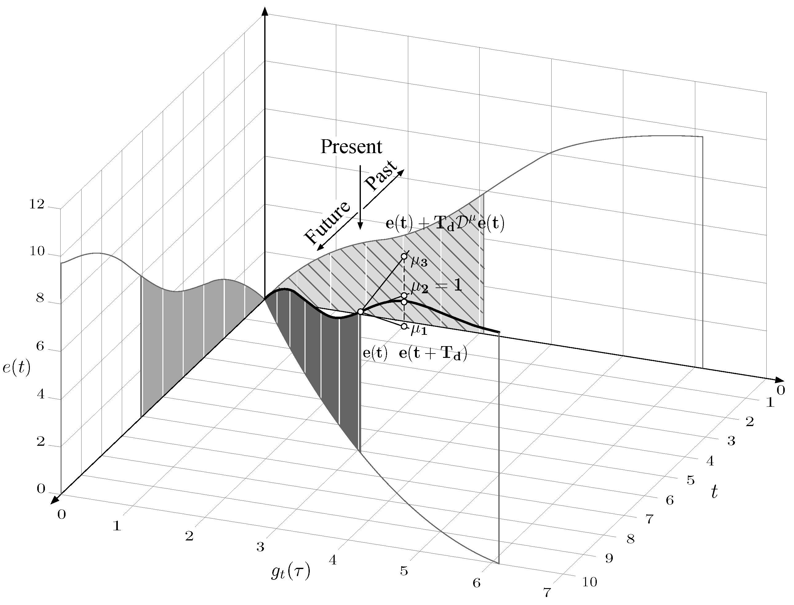
Figure 2 is an attempt to illustrate these effects. It should be remarked that, in this figure, the error was considered as the function (taken from [51]). To show the integral and derivative effects for non-integer orders, it must be said that:
- For integral action, left-side Riemann-Liouville fractional integral of the error was considered as:whereThen, taking the axes , and e, function was plotted in the plane for . Along the obtained curve, a “fence” was plotted varying , so the top edge of the “fence” is a 3D line for . The area of the projection of this “fence” onto the plane corresponds to the value of the integer order integral of the error (i.e., the classical area under the curve), whereas that of the projection onto the plane corresponds to the value of fractional order integral (4). All this reasoning was adapted from [51].
- For derivative action, straight lines that pass through the point and whose slope matches the value of the differentiation of order of the error curve at that point were plotted.
The following values of the orders were taken for simulations: , , , and .
3. Going Into Detail About Parameters
This section contains the explanation of the meaning of the parameters of FOPID controllers, in comparison with those classical of integer order. It should be remarked that, despite the fact the proportional action is not affected by a fractional order, it is also included for completeness of information.
3.1. Proportional Action
The proportional action increases the deviation between the set-point value and the system output y (i.e., the error) with the proportional gain . The main drawback of using a pure proportional control action is that it produces a steady-state error, which motivates that it can be also considered as:
where is a bias or reset [4]. Indeed, when , the control signal reduces to . The parameter usually takes the value , where and are the maximum and minimum limits of the actuator, respectively. However, sometimes can be adjusted manually to a value that ensures that the steady-state error is zero at a given set-point.
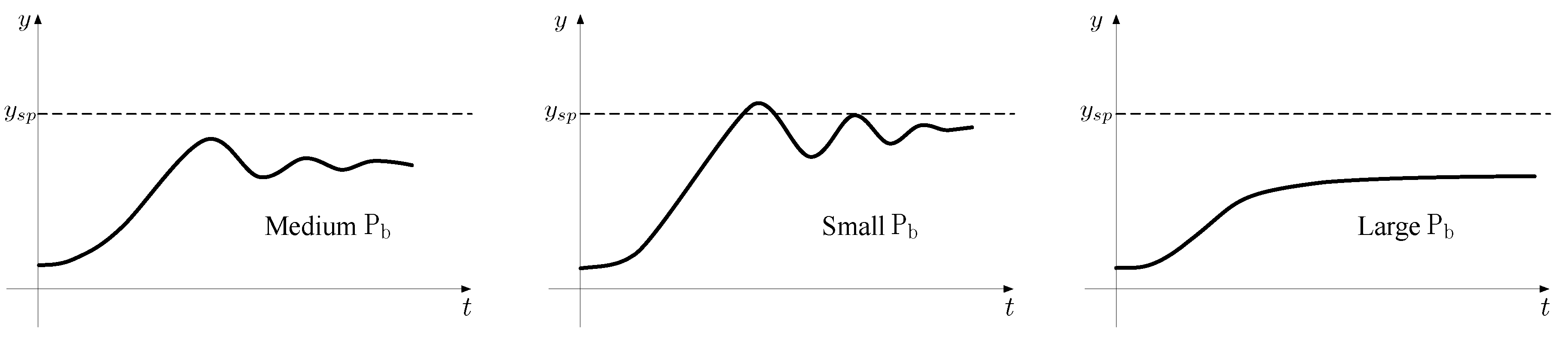
Likewise, the proportional gain can be specified in terms of its inverse proportional band, , which represents the percentage of change in the error signal necessary to cause a full-scale change in the proportional action. As can be observed in Figure 3, the tendency of y to oscillate increases as decreases. The large oscillations occurring with a small are due to the fact that the power is reduced very quickly when the system output enters the proportional band, meaning a balanced state cannot be established immediately.
Indeed, confusing “proportional band” with “proportional gain” leads to a decreased proportional action when the control engineer wants more, and vice-versa.
3.2. Integral Action
The main function of the integral action is to guarantee that the steady-state error is zero, i.e., the output of the controlled system is equal to the desired set-point in steady-state. The following simple explanation proves this affirmation. Let us consider a system controlled by a fractional order proportional-integral (PI) controller in steady-state where both the control signal () and the error () are constant. If this is the case, the control signal will be given by [3]
While , this clearly contradicts the hypothesis that the control signal is constant. Thus, similarly to the integer case, a controller with integral action of fractional order will always give zero error in steady-state.
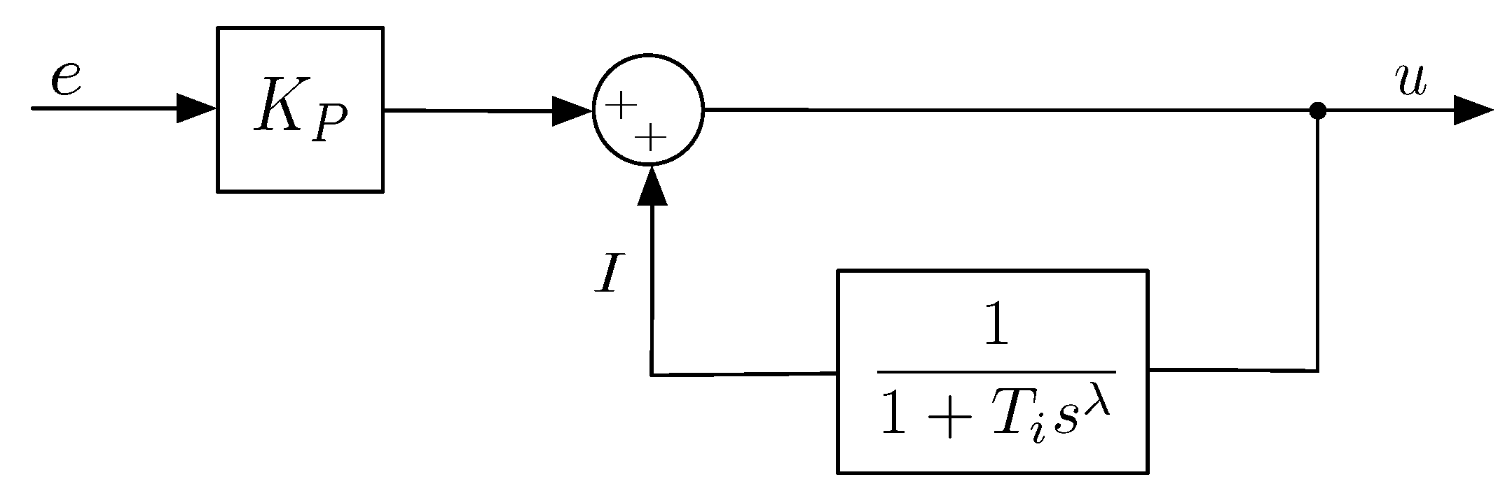
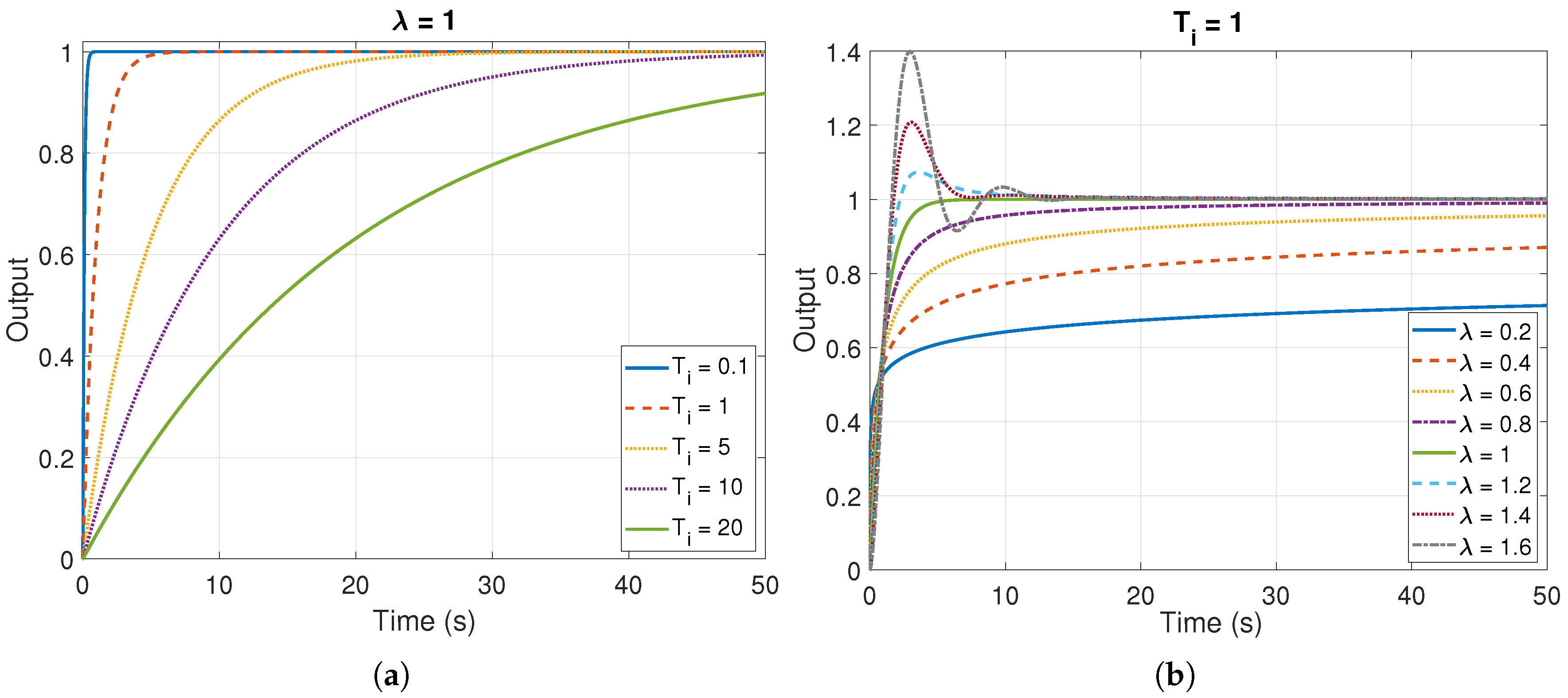
Integral action was known originally as a device that automatically resets the bias of a proportional controller. Figure 4 shows the scheme of the extension to non-integer orders of a PI controller with automatic reset. As can be observed, the first order filter in the feedback loop is replaced by its fractional version of order . From the block diagram, the control signal can be obtained as
with
Substituting (9) in (8), the control signal is given by
thus the control scheme of the figure is equivalent to a fractional order PI controller. Figure 5 shows unit step responses of the fractional system in the feedback loop in Figure 4. Unlike the integer order case (see Figure 5a), both the velocity and the shape of resetting can be controlled by the integration order, , as shown in Figure 5b. It can be observed that it is even possible to obtain underdamped responses when .
It is important to remark that function fode_sol() was taken from [10] to obtain the step responses in MATLAB.
3.3. Derivative Action
The objective of the derivative action is to improve the system stability in closed-loop. Classical derivative controllers give responses to changing error signals but do not, however, respond to constant error signals, since with a constant error the rate of change of error with time is zero. Because of this, the derivative term is combined with, at least, the proportional term. By contrast, fractional derivative controllers do response to constant error signals; the differentiation of fractional order of a constant is different from zero.
The derivative action of a proportional-derivative (PD) controller can be viewed as a crude prediction of the error in future, where the prediction is made by extrapolating the error by the tangent to the error curve at time t, being the prediction horizon (see Figure 1). (Actually, the derivative action uses linear extrapolation, not prediction.) For the fractional case, the basic structure of the controller is
Analogously to the classical case, an approximation of may be
The control signal is then proportional to an estimation of the error at time ahead over a straight line that, in general, is not tangent to the error curve, and whose slope matches the value of the differentiation of -th order of the error curve at the point [52], as shown in Figure 2. Likewise, another way of viewing the prediction is from fractional Taylor series for fractional derivatives. In this case, the prediction horizon is done over a curve (i.e., non-linear extrapolation). More details about prediction can be found in Appendix A.
Therefore, different prediction horizons (in fact, linear and non-linear extrapolations) for the error can be obtained choosing accordingly the value of .
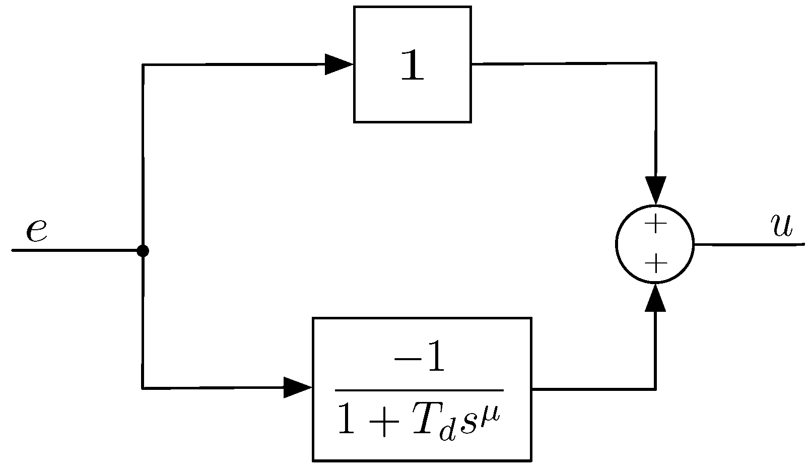
The classical implementation of a fractional derivative action is illustrated in Figure 6. From this figure, the following relation can be obtained
which corresponds to a derivative action of fractional order with noise filter. It is well known that the derivative part of the PID controller requires low-pass filtering to limit the high-frequency gain.
Let us focus only on the noise filter of (13), i.e.,
Notice that: (1) it has the property to ensure that the process output equals the set-point in steady-state; (2) as usual, it has a low-pass character; and (3) the order of the filter is .
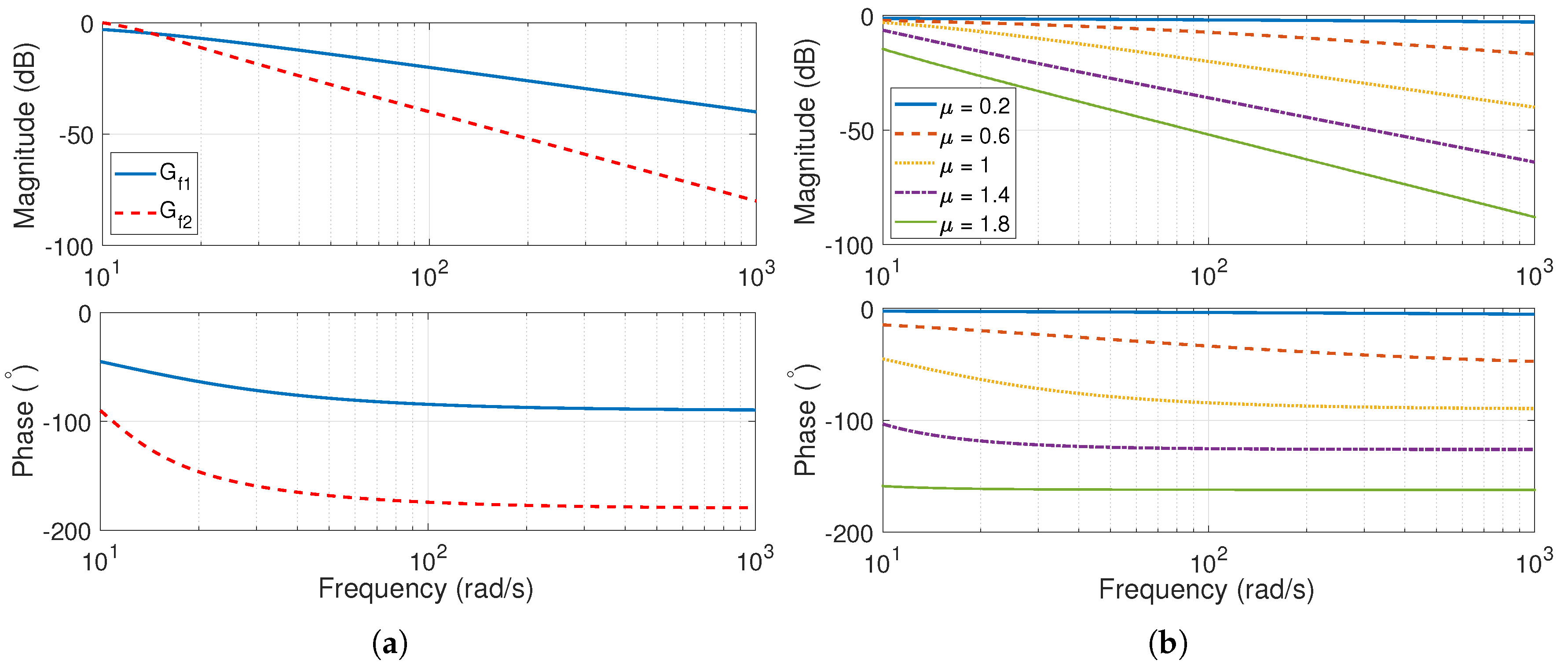
In the literature, the classical filters to reduce noise effects in PID controllers are up to second order, usually given as follows [54]:
where is the filter time constant. Note that filter (16) has complex poles with damping ratio .
Figure 7 shows Bode plots of the filters, of both integer and fractional order, for . As can be seen in Figure 7b, changes in the order allow to have different frequency responses ranged between those of the two integer filters (Figure 7a), and consequently, different filtering effects on the error signal can be attained. Another issue to take into account is that most design methods for classical PIDs do not consider noise. Due to this fact, the filter time constant is often suggested to be chosen as a fraction of the derivative time, i.e., . However, this solution has severe drawbacks, as reported in [55]. On the contrary, this is not necessary for the fractional case because there is an only parameter to be tuned, , and it is included in the controller design.
4. Classical Versus Fractional PIDs
This section discusses the similarities and differences between classical and fractional PIDs. In particular, only integral and derivatives parts are compared— the proportional part is similar for both kinds of controllers. The properties described below are summarized in Table 1.
4.1. Integral Part
As is well known, the main effects of the integral action are those that make the system response slower, decrease its relative stability, and eliminate the steady-state error for inputs for which previously had a finite error. These effects can be observed in the different domains of analysis as follows. In the time-domain, the effects on the transient response cause a decrease of the rising time and an increase of the settling time and the overshoot. In the complex plane, the integral action causes a displacement of the root locus of the system towards the right half-plane. Finally, in the frequency-domain, an increase of dB/dec in the slopes of the magnitude curves and a decrement of in the phase plots can be observed.
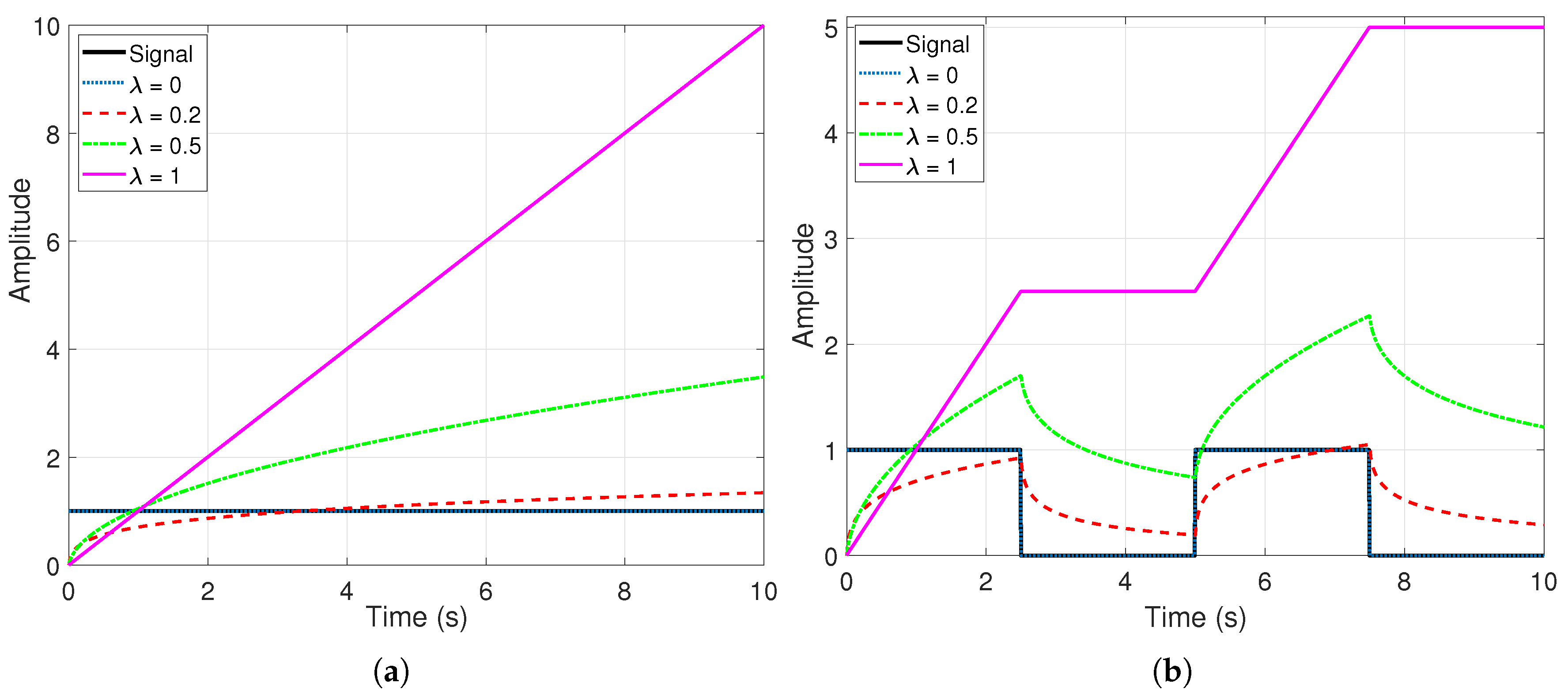
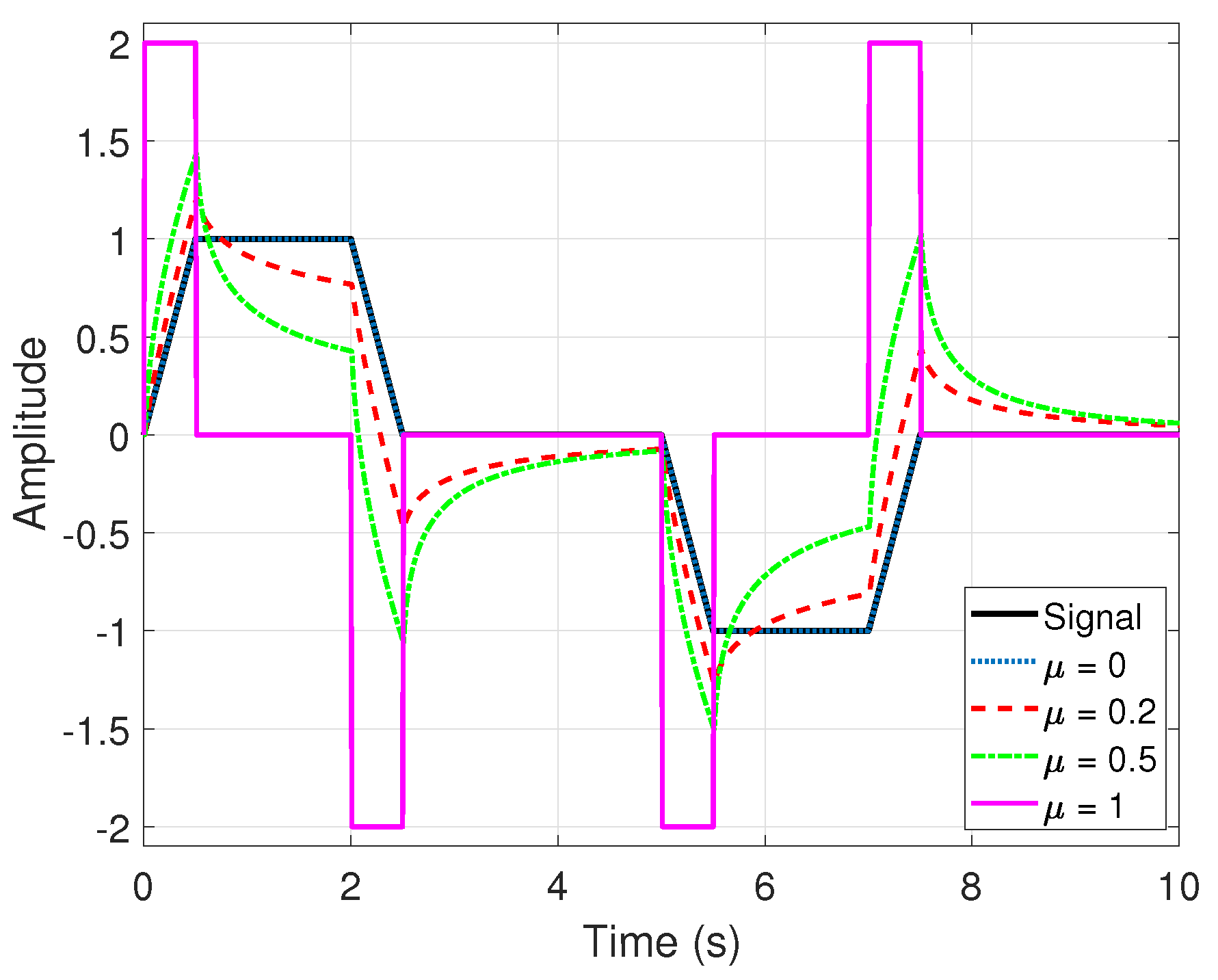
In the case of a fractional integration order , the selection of the value of translates into a certain weighting of the effects mentioned above. In the time-domain, for example, due to the fact that the integral action only responds to errors other than zero by increasing the control action, for positive errors, and decreasing it in case of negative, if the error is constant, the control action can be ramped up with different slopes or velocities, as can be observed in Figure 8a. For a square error signal (Figure 8b), it can be observed that there is a set of effects of the control action over the error that range from the pure proportional action () to the classical integral action (). For intermediate values of , the control action grows when the error is constant, which results in a removal of the steady-state error, whereas decreases when the error goes to zero, which reduces the instability of the system. In the complex plane, it can be seen that the selection of a value of parameter moves the root locus of the system towards the right half-plane. In the frequency-domain, the fact that can vary between 0 and 1 introduces the possibility of adding a constant increment to the slope of the magnitude curve between 0 and dB/dec (actually, a value of dB/dec), as well as a constant lag to the phase curve between 0 and rad (specifically, a value of rad).
4.2. Derivative Part
The derivative action increases the system stability and tends to accentuate the noise effects at high frequencies. In the time-domain, this is manifested, mainly, by a decrease in both the overshoot and the settling time. In the complex plane, it produces a displacement of the system root locus towards the left half-plane. In the frequency-domain, a constant phase lead of /2 and an increase of 20 dB/dec in the slopes of the magnitude curves.
Following a reasoning parallel to that made for the integral action, it is easy to understand that all these effects are weighted by choosing an appropriate value of the order of the derivative, (see Figure 9).
5. Illustrative Examples
This section provides two examples to illustrate the properties of both integral and derivative actions, as well the effects of their fractional orders.
Example 1.
Let us consider a system given by the following transfer function [4]
controlled by a fractional order PI of the form:
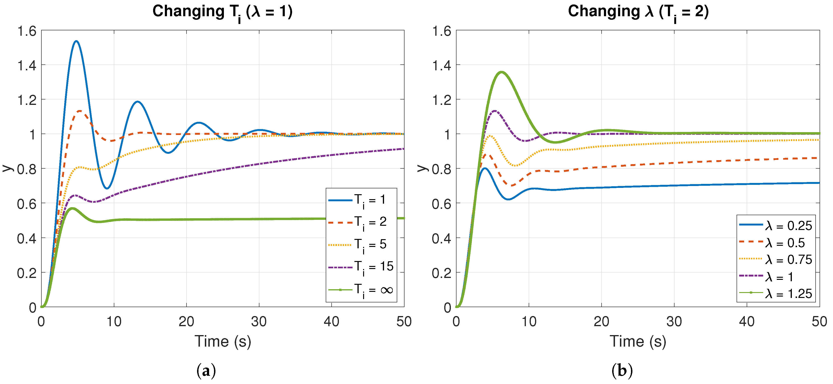
To illustrate the properties of the integral action and the effect of its fractional order, Figure 10 shows unit step responses in closed-loop of system (17) controlled by fractional PI controller (18). The proportional gain is constant, , whereas the integral time and are changed individually in Figure 10a,b, respectively. More precisely, responses for the classical case () are plotted in Figure 10a. As expected, the steady-state error is removed when takes finite values; the case corresponds to pure proportional control, where the steady-state error is 50 percent. Likewise, the smaller the values of , the faster the response, but the more oscillatory [4]. The effects of changing the integration order, , can be seen in Figure 10b ( is fixed to 2). In this case, the smaller the values of , the slower the response. Unlike , oscillations and system response are not affected by parameter .
Example 2.
Now, consider the double integrator with unit gain, i.e.,
controlled by a fractional order PD of the form:
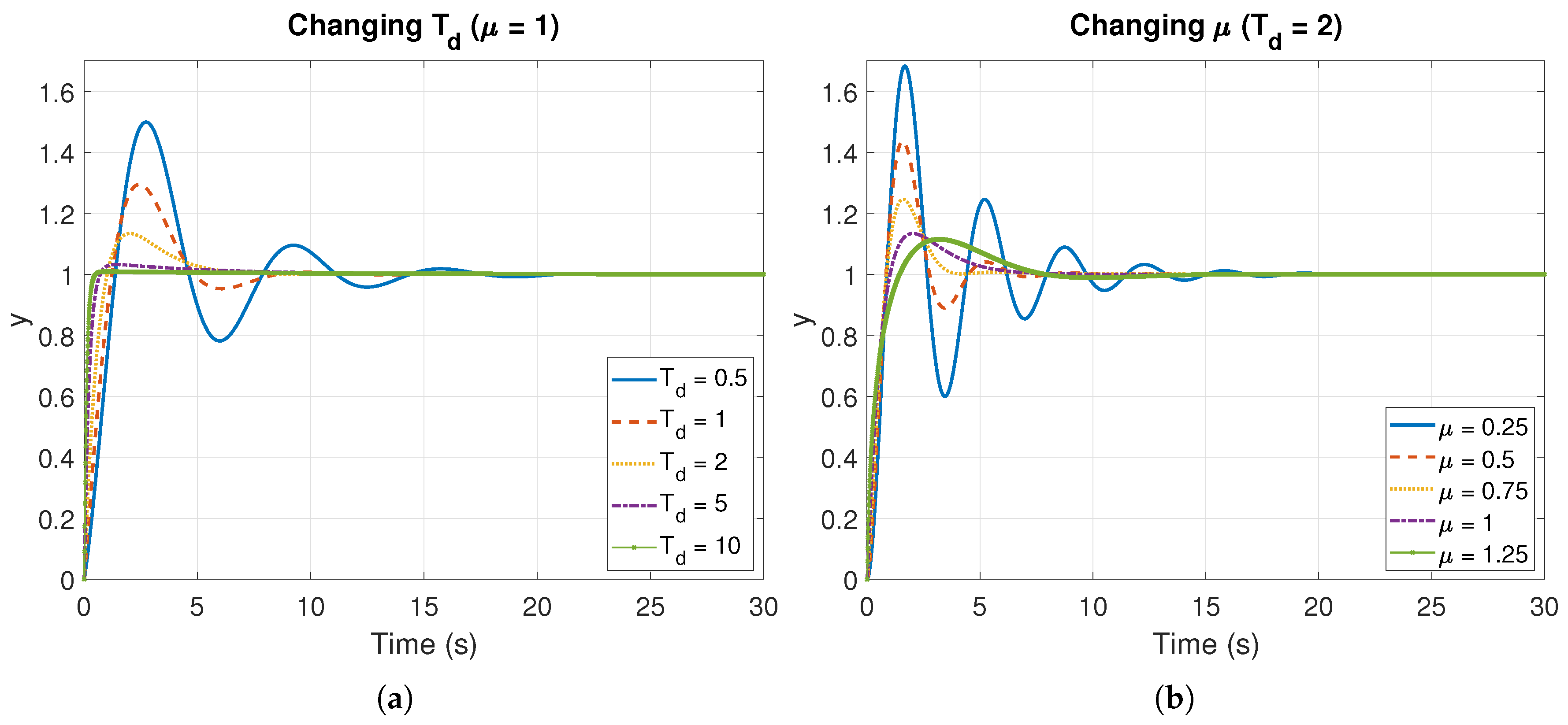
The properties of the derivative action and its non-integer order are illustrated in Figure 11, which shows unit step responses in closed-loop of system (19) controlled by fractional PD controller (20). Similarly to the previous example, the proportional gain is constant, , whereas the derivative time and are changed in an individual way in Figure 11a,b, respectively. In particular, responses for the classical case () are plotted in Figure 11a. As expected, damping increases when increases. In other words, the higher the values of , the faster the response. The effects of changing can be observed in Figure 11b ( is set to 2). In this case, the smaller the values of , the slower the damping. Unlike , only affects the overshoot.
It must be said that the function fode_sol() was also used to obtain the step responses of both examples.
6. Conclusions
Although ample studied and successfully applied to many kinds of control problems, the extension of classical proportional-integral-derivative (PID) controllers to non-integer orders presents a main weakness: basis, in terms of understanding of the effects of their parameters on the system response, is sometimes omitted, and even unknown. This can be explained, in part, because the geometric and physical interpretation of integrals and derivatives of arbitrary (not necessary integer) order still remains as an open problem. This paper has focused on the new meaning of integral and derivative actions, and gains, derived by the consideration of non-integer integration and differentiation orders, i.e., for fractional order PID (FOPID) controllers. Similarities and differences between classical and fractional PIDs, as well as illustrative examples were given for a best understanding of the possibilities of control with the latter.
When the integral term is concerned, it was shown that it responds with selective memory because of the non-integer order . That was also viewed as the area of the projection of the error curve onto a plane, which is definitively different from the classical area under the error curve. Moreover, taking into account a fractional proportional-integral (PI) controller scheme with automatic reset, unlike the integer order case, it was also shown that both the velocity and the shape of resetting can be controlled by the integration order, .
With respect to derivative action, it was illustrated that different prediction horizons (in fact, linear and non-linear extrapolations) for the error can be obtained for a fractional proportional-derivative (PD) choosing accordingly the value of the differentiation order, . Likewise, in case of an structure with noise filter, the value of allows different filtering effects on the error signal to be attained.
Author Contributions
This work involved all coauthors. I.T. wrote the original draft and contributed to the investigation and the analysis, edited the manuscript and contributed to the illustrations and examples. B.M.V. conceived the idea, contributed to the editing and supervised all the manuscript. J.E.T. wrote the plotting software and contributed to the illustrations. J.P.-A. and C.N.-G. contributed to the illustrations and the editing.
Funding
This research has been supported in part by the Spanish Agencia Estatal de Investigación (AEI) under Project DPI2016-80547-R (Ministerio de Economía y Competitividad), and in part by the European Social Fund (FEDER, EU).
Conflicts of Interest
The authors declare no conflict of interest.
Appendix A. Analysis of Prediction Horizon
This appendix gives information about the approximation of the prediction of the error at time ahead, i.e., the approximation of to understand the meaning of a fractional order derivative action.
Let assume that the error is a continuous function, and , , where h is a fixed step. Thus, can be approximated by:
which is referred to as approximation #1. Likewise, analogously with the integer case, the prediction may be also expressed as
It is referred to as approximation #2.
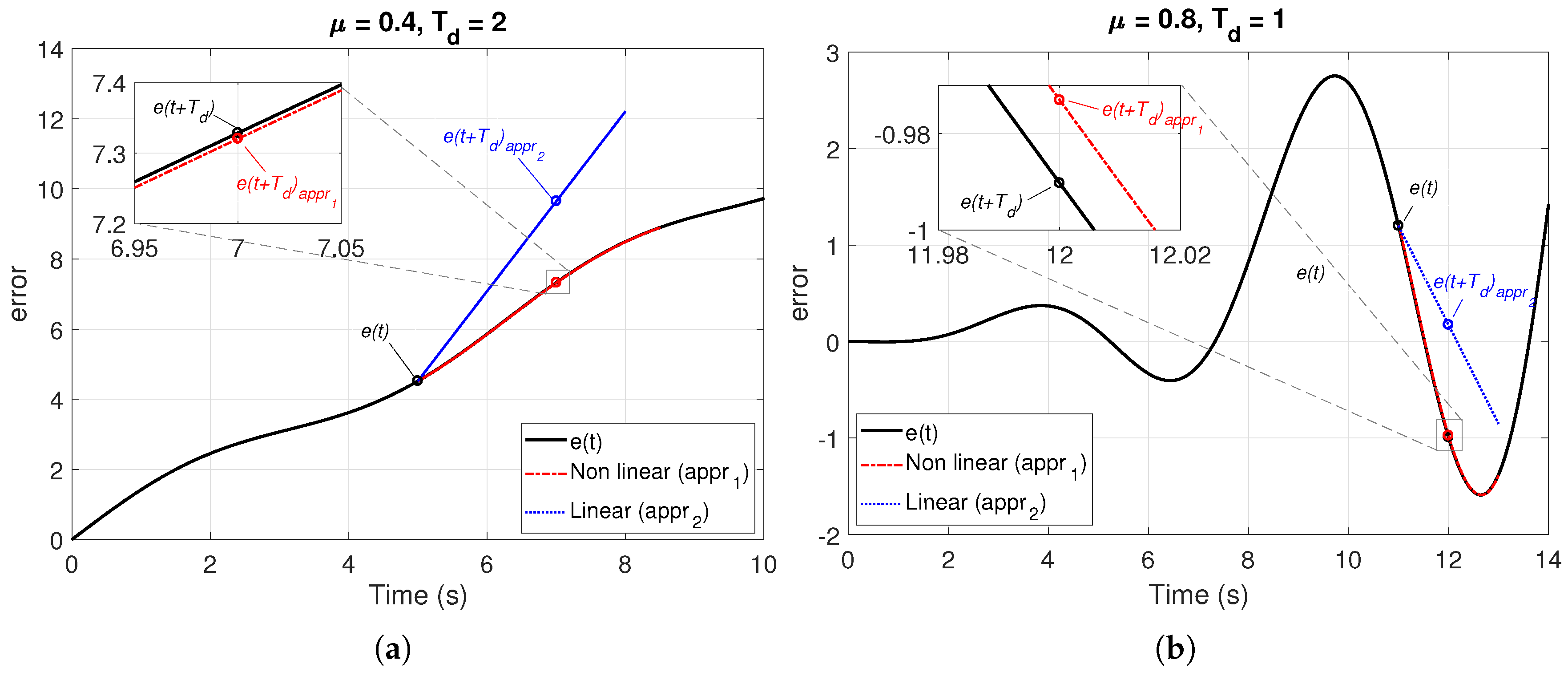
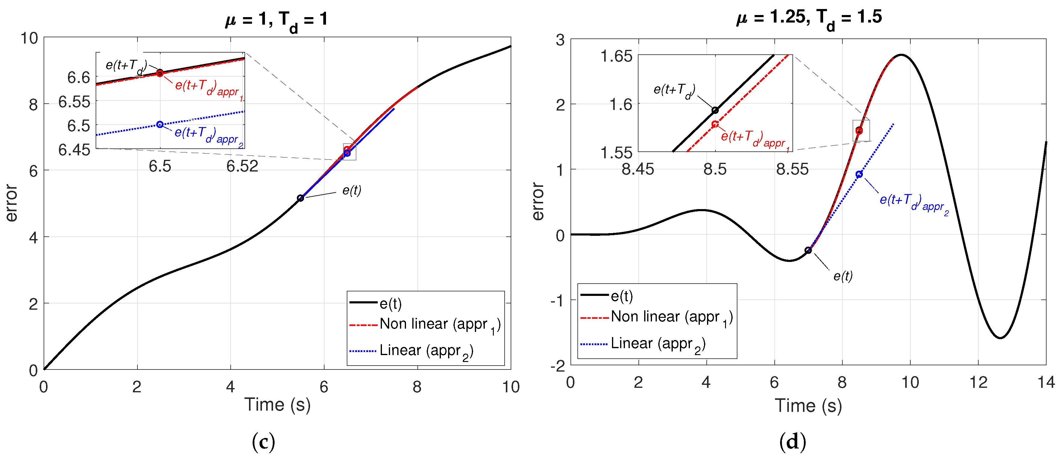
Hence, taking into account approximation #1, the prediction in future of the error is done from a non-linear extrapolation due to the fact that the term on the right in (A2) is non-linear. In contrast, the prediction with (A3) is carried out over a straight line (linear extrapolation) that passes for point t, and whose slope matches the value of the -th order differentiation of the error. Thus, the control signal is proportional to an estimation of the control error at time ahead, where that estimation is obtained by non-linear or linear extrapolation. Both predictions are illustrated in Figure A1 for different values of and , namely, and , and considering the error as and . As can be observed, although there are big differences between the approximations above, the prediction function assumed to the derivative term is guaranteed at time ahead, especially when approximation given by (A2) is taken: it approaches, to a large extent, the actual curve of the error.
Figure A1.
Prediction horizons of derivative part depending on the order : (a) , (b) , (c) , (d) , . Notice that cases (a) and (c) correspond to the error as the function , whereas the error is given by in cases (b) and (d).
Figure A1.
Prediction horizons of derivative part depending on the order : (a) , (b) , (c) , (d) , . Notice that cases (a) and (c) correspond to the error as the function , whereas the error is given by in cases (b) and (d).


References
- Aström, K.J.; Hägglund, T. PID Controllers: Theory, Design and Tuning, 2nd ed.; ISA—The Instrumentation, Systems, and Automation Society: Research Triangle Park, NC, USA, 1995. [Google Scholar]
- Aström, K.J.; Murray, R.M. Feedback Systems: An Introduction for Scientists and Engineers, 2nd ed.; Princeton University Press: Princeton, NJ, USA, 2008. [Google Scholar]
- Podlubny, I. Fractional-order systems and PIλDμ-controllers. IEEE Trans. Autom. Control 1999, 44, 208–214. [Google Scholar] [CrossRef]
- Aström, K.J.; Hägglund, T. Advanced PID Control; Chapter PID Control; ISA—The Instrumentation, Systems, and Automation Society: Research Triangle Park, NC, USA, 2006; pp. 64–94. [Google Scholar]
- Visioli, A. Practical PID Control; Advances in Industrial Control; Chapter Basics of PID Control; Springer: Berlin/Heidelberg, Germany, 2006; pp. 1–18. [Google Scholar]
- Li, Y.; Heong, K.; Chong, G.C.Y. PID Control System Analysis and Design. Problems, Remedies, and Future Directions. IEEE Control Syst. Mag. 2006, 26, 32–41. [Google Scholar]
- Vinagre, B.M.; Feliu-Batlle, V.; Tejado, I. Fractional Control: Fundamentals and User Guide. Revista Iberoamericana de Automática e Informática Industrial 2016, 13, 265–280. [Google Scholar] [CrossRef]
- Valério, D.; Sá da Costa, J. An Introduction to Fractional Control; IET Control Engineering, The Institution of Engineering and Technology: Stevenage, UK, 2013. [Google Scholar]
- Vinagre, B.M.; Monje, C.A. PID Control in the Third Millennium. Lessons Learned and New Approaches; Advances in Industrial Control; Chapter Fractional-Order PID; Springer: Berlin/Heidelberg, Germany, 2012; pp. 465–494. [Google Scholar]
- Monje, C.A.; Chen, Y.Q.; Vinagre, B.M.; Xue, D.; Feliu, V. Fractional-Order Systems and Controls. Fundamentals and Applications; Springer: Berlin/Heidelberg, Germany, 2010. [Google Scholar]
- Lorenzini, C.; Bazanella, A.S.; Alves Pereira, L.F.; Goncalves da Silva, G.R. The generalized forced oscillation method for tuning PID controllers. ISA Trans. 2019, 87, 68–87. [Google Scholar] [CrossRef] [PubMed]
- Tajjudin, M.; Rahiman, M.H.F.; Arshad, N.M.; Adnan, R. Robust Fractional-Order PI Controller with Ziegler-Nichols Rules. Int. J. Electr. Comput. Eng. 2013, 7, 1034–1041. [Google Scholar]
- Gude, J.J.; Kahoraho, E. Modified Ziegler-Nichols method for fractional PI controllers. In Proceedings of the 2010 IEEE 15th Conference on Emerging Technologies & Factory Automation (ETFA 2010), Bilbao, Spain, 13–16 September 2010. [Google Scholar]
- Valério, D.; Sá da Costa, J. Tuning of fractional PID controllers with Ziegler-Nichols-type rules. Signal Process. 2006, 10, 2771–2784. [Google Scholar] [CrossRef]
- Hekimoglu, B. Optimal Tuning of Fractional Order PID Controller for DC Motor Speed Control via Chaotic Atom Search Optimization Algorithm. IEEE Access 2019, 7, 38100–38114. [Google Scholar] [CrossRef]
- Kesarkar, A.A.; Selvaganesan, N. Tuning of optimal fractional-order PID controller using an artificial bee colony algorithm. Syst. Sci. Control Eng. 2015, 3, 99–105. [Google Scholar] [CrossRef]
- Padula, F.; Visioli, A. Tuning rules for optimal PID and fractional-order PID controllers. J. Process Control 2011, 21, 69–81. [Google Scholar] [CrossRef]
- Biswas, A.; Das, S.; Abraham, A.; Dasgupta, S. Design of fractional-order PIλDμ controllers with an improved differential evolution. Eng. Appl. Artif. Intell. 2009, 22, 343–350. [Google Scholar] [CrossRef]
- Liu, L.; Zhang, S. Robust Fractional-Order PID Controller Tuning Based on Bode’s Optimal Loop Shaping. Complexity 2018, 2018, 6570560. [Google Scholar] [CrossRef]
- HosseinNia, S.H.; Tejado, I.; Vinagre, B.M. A Method for the Design of Robust Controllers Ensuring the Quadratic Stability for Switching Systems. J. Vib. Control 2014, 20, 1085–1098. [Google Scholar] [CrossRef]
- Monje, C.A.; Calderón, A.J.; Vinagre, B.M.; Chen, Y.Q.; Feliu, V. On fractional PIλ controllers: Some tuning rules for robustness to plant uncertainties. Nonlinear Dyn. 2004, 38, 369–381. [Google Scholar] [CrossRef]
- De Keyser, R.; Muresan, C.I.; Ionescu, C.M. A novel auto-tuning method for fractional order PI/PD controllers. ISA Trans. 2016, 62, 268–275. [Google Scholar] [CrossRef] [PubMed]
- Monje, C.A.; Vinagre, B.M.; Feliu, V.; Chen, Y.Q. Tuning and auto-tuning of fractional order controllers for industry applications. Control Eng. Pract. 2008, 16, 798–812. [Google Scholar] [CrossRef] [Green Version]
- Chevalier, A.; Francis, C.; Copot, C.; Ionescu, C.M.; De Keyser, R. Fractional-order PID design: Towards transition from state-of-art to state-of-use. ISA Trans. 2019, 84, 178–186. [Google Scholar] [CrossRef] [PubMed]
- Feliu-Batlle, V.; Rivas-Perez, R.; Castillo-Garcia, F.J. Simple Fractional Order Controller Combined with a Smith Predictor for Temperature Control in a Steel Slab Reheating Furnace. Int. J. Control Autom. Syst. 2013, 11, 533–544. [Google Scholar] [CrossRef]
- Feliu-Battle, V.; Rivas Pérez, R.; Castillo García, F.J.; Sánchez Rodríguez, L. Smith predictor based robust fractional order control: Application to water distribution in a main irrigation canal pool. J. Process Control 2009, 19, 506–519. [Google Scholar] [CrossRef]
- Luan Vu, T.N.; Lee, M. Smith predictor based fractional-order PI control for time-delay processes. Korean J. Chem. Eng. 2014, 31, 1321–1329. [Google Scholar]
- Lakshmanaprabu, S.K.; Banu, U.S.; Hemavathy, P.R. Fractional order IMC based PID controller design using Novel Bat optimization algorithm for TITO Process. Energy Proc. 2017, 117, 1125–1133. [Google Scholar] [CrossRef]
- Muresan, C.I.; Dutta, A.; Dulf, E.H.; Pinar, Z.; Maxim, A.; Ionescu, C.M. Tuning algorithms for fractional order internal model controllers for time delay processes. Int. J. Control 2016, 89, 579–593. [Google Scholar] [CrossRef]
- Maamar, B.; Rachid, M. IMC-PID-fractional-order-filter controllers design for integer order systems. ISA Trans. 2014, 53, 1620–1628. [Google Scholar] [CrossRef] [PubMed]
- HosseinNia, S.H.; Tejado, I.; Vinagre, B.M.; Milanés, V.; Villagrá, J. Experimental Application of Hybrid Fractional Order Adaptive Cruise Control at Low Speed. IEEE Trans. Control Syst. Technol. 2014, 22, 2329–2336. [Google Scholar] [CrossRef]
- Ahmed, M.F.; Dorrah, H.T. Design of gain schedule fractional PID control for nonlinear thrust vector control missile with uncertainty. Automatika 2018, 59, 357–372. [Google Scholar] [CrossRef]
- Tejado, I.; Milanés, V.; Villagrá, J.; Vinagre, B.M. Fractional Network-based Control for Vehicle Speed Adaptation via vehicle-to-infrastructure Communications. IEEE Trans. Control Syst. Technol. 2013, 21, 780–790. [Google Scholar] [CrossRef]
- Tejado, I.; HosseinNia, S.H.; Vinagre, B.M.; Chen, Y.Q. Efficient control of a SmartWheel via Internet with compensation of variable delays. Mechatronics 2013, 23, 821–827. [Google Scholar] [CrossRef]
- Tejado, I.; HosseinNia, S.H.; Vinagre, B.M. Adaptive gain-order fractional control for network-based applications. Fract. Calc. Appl. Anal. 2014, 17, 462–482. [Google Scholar] [CrossRef]
- Pan, I.; Das, S. Intelligent Fractional Order Systems and Control; Chapter Gain and Order Scheduling for Fractional Order Controllers; Springer: Berlin/Heidelberg, Germany, 2013; pp. 147–157. [Google Scholar]
- Dastjerdi, A.A.; Vinagre, B.M.; Chen, Y.Q.; HosseinNia, S.H. Linear fractional order controllers; A survey in the frequency domain. Ann. Rev. Control 2019. [Google Scholar] [CrossRef]
- Birs, I.; Muresan, C.; Nascu, I.; Ionescu, C. A Survey of Recent Advances in Fractional Order Control for Time Delay Systems. IEEE Access 2019, 7, 30951–30965. [Google Scholar] [CrossRef]
- Petrás, I. Handbook of Fractional Calculus with Applications; Chapter Modified Versions of the Fractional-Order PID Controller; De Gruyter: Berlin, Germany, 2019; Volume 6, pp. 57–72. [Google Scholar]
- Dastjerdi, A.A.; Saikumar, N.; HosseinNia, S.H. Tuning guidelines for fractional order PID controllers: Rules of thumb. Mechatronics 2018, 56, 26–36. [Google Scholar] [CrossRef]
- Tepljakov, A.; Alagoz, B.B.; Yeroglu, C.; Gonzalez, E.; HosseinNia, S.H.; Petlenkov, E. FOPID Controllers and Their Industrial Applications: A Survey of Recent Results. In Proceedings of the 3rd IFAC Conference on Advances in Proportional-Integral-Derivative Control, Ghent, Belgium, 9–11 May 2018; Volume 51, pp. 25–30. [Google Scholar]
- Shah, P.; Agashe, S. Review of fractional PID controller. Mechatronics 2016, 38, 29–41. [Google Scholar] [CrossRef]
- Apte, A.; Thakar, U.; Joshi, V. Disturbance Observer Based Speed Control of PMSM Using Fractional Order PI Controller. IEEE-CAA J. Autom. Sin. 2019, 6, 316–326. [Google Scholar] [CrossRef]
- AbouOmar, M.S.; Zhang, H.J.; Su, Y.X. Fractional Order Fuzzy PID Control of Automotive PEM Fuel Cell Air Feed System Using Neural Network Optimization Algorithm. Energies 2019, 12, 1435. [Google Scholar] [CrossRef]
- Copot, D.; Ghita, M.; Ionescu, C.M. Simple Alternatives to PID-Type Control for Processes with Variable Time-Delay. Processes 2019, 7, 146. [Google Scholar] [CrossRef]
- Deng, Y. Fractional-order fuzzy adaptive controller design for uncertain robotic manipulators. Int. J. Adv. Robot. Syst. 2019, 16, 1–10. [Google Scholar] [CrossRef]
- Feliu-Talegon, D.; Feliu-Batlle, V.; Tejado, I.; Vinagre, B.M.; HosseinNia, S.H. Stable force control and contact transition of a single link flexible robot using a fractional-order controller. ISA Trans. 2019, 89, 139–157. [Google Scholar] [CrossRef] [PubMed]
- Ren, H.P.; Fan, J.T.; Kaynak, O. Optimal Design of a Fractional-Order Proportional-Integer-Differential Controller for a Pneumatic Position Servo System. IEEE Trans. Ind. Electr. 2019, 66, 6220–6229. [Google Scholar] [CrossRef]
- Zhang, F.; Yang, C.; Zhou, X.; Gui, W. Optimal Setting and Control Strategy for Industrial Process Based on Discrete-Time Fractional-Order (PID mu)-D-lambda. IEEE Access 2019, 7, 47747–47761. [Google Scholar] [CrossRef]
- Mystkowski, A.; Kierdelewicz, A. Fractional-order water level control based on PLC: hardware-in-the-loop simulation and experimental validation. Energies 2018, 11, 2928. [Google Scholar] [CrossRef]
- Podlubny, I. Geometric and Physical Interpretation of Fractional Integration and Fractional Differentiation. Fract. Calc. Appl. Anal. 2004, 5, 367–386. [Google Scholar]
- Tavassoli, M.H.; Tavassoli, A.; Rahimi, M.R.O. The geometric and physical interpretation of fractional order derivatives of polynomial functions. Differ. Geom. Dyn. Syst. 2013, 15, 93–104. [Google Scholar]
- Podlubny, I. Fractional Differential Equations. An Introduction to Fractional Derivatives, Fractional Differential Equations, to Methods of Their Solution and Some of Their Applications; Mathematics in Science and Engineering; Academic Press: Cambridge, MA, USA, 1999; Volume 198. [Google Scholar]
- Hägglund, T. A unified discussion on signal filtering in PID control. Control Eng. Pract. 2013, 21, 994–1006. [Google Scholar] [CrossRef]
- Isaksson, A.; Graebe, S. Derivative filter is an integral part of PID design. IEE Proc. Control Theor. Appl. 2002, 149, 41–45. [Google Scholar] [CrossRef]
- Fractional Taylor Series for Caputo Fractional Derivatives. Construction of Numerical Schemes. Available online: http://www.fdi.ucm.es/profesor/lvazquez/calcfrac/docs/paper_Usero.pdf (accessed on 22 April 2019).
Figure 1.
Evolution of the error (classical proportional-integral-derivative (PID) controllers).

Figure 2.
Evolution of the error (fractional PID controllers).

Figure 3.
System response for different .

Figure 4.
Fractional proportional-integral (PI) controller scheme (classical implementation with automatic reset).
Figure 4.
Fractional proportional-integral (PI) controller scheme (classical implementation with automatic reset).

Figure 5.
Effects of the automatic reset of the integral action when changing: (a) integral time constant (integer case) (b) integration order (fractional case).
Figure 5.
Effects of the automatic reset of the integral action when changing: (a) integral time constant (integer case) (b) integration order (fractional case).

Figure 6.
Fractional order derivative action scheme (classical implementation).

Figure 7.
Frequency response of the noise filter: (a) first and second order low-pass filters (integer case) (b) fractional filter for different values of (fractional case). For simulations, the following values were taken: .
Figure 7.
Frequency response of the noise filter: (a) first and second order low-pass filters (integer case) (b) fractional filter for different values of (fractional case). For simulations, the following values were taken: .

Figure 8.
Effects of the integral action according to integration order on different error signals: (a) constant (b) square.
Figure 8.
Effects of the integral action according to integration order on different error signals: (a) constant (b) square.

Figure 9.
Effects of the derivative action according to differentiation order on a trapezoidal signal.
Figure 9.
Effects of the derivative action according to differentiation order on a trapezoidal signal.

Figure 10.
Step responses in closed-loop of system (17) controlled by fractional PI controller (18) when changing: (a) integral time constant (, ) (b) integration order (, ).

Figure 11.
Step responses in closed-loop of system (19) controlled by fractional PD controller (20) when changing: (a) derivative time constant (, ) (b) integration order (, ).


Table 1.
Similarities and differences between classical and fractional proportional-integral-derivatives (PID) controllers.
Table 1.
Similarities and differences between classical and fractional proportional-integral-derivatives (PID) controllers.
| Action | Domain | Effect on | Integer | Fractional |
|---|---|---|---|---|
| I | Time | Steady-state error | Elimination | |
| u with respect to the sign of e | If , u grows linearly with time | The same but the growing or the decrease is not linear with time | ||
| If , u decreases linearly with time | ||||
| Automatic reset | The velocity of reset can be changed | Both the velocity and the shape of reset can be changed | ||
| Frequency | Frequency response | The magnitude curve decreases with a slope of 20 dB/dec | The magnitude curve decreases with a slope of dB/dec | |
| Decrease of rad in the phase curve | Decrease of rad in the phase curve | |||
| D | Time | Constant errors | Does not response, so the derivative term needs to be combined with, at least, the proportional term | Does response, so the derivative term can be used individually |
| Prediction horizon | Time ahead over the tangent to the error curve at | Time ahead over a curve (non-linear extrapolation) or over a straight line (linear extrapolation) that passes through the point and whose slope matches the value of the fractional differentiation of order of the error curve at that point | ||
| Frequency | Frequency response | The magnitude curve grows with a slope of 20 dB/dec | The magnitude curve grows with a slope of dB/dec | |
| Increment of rad in the phase curve | Increment of rad in the phase curve | |||
| Filtering | Low-pass filters up to second order | Low-pass filter of order | ||
| Usually needs two parameters to be tuned, i.e., (filter time constant) and N (ratio between and ) | Parameter allows to have different frequency responses, ranged between those of the two integer filters, and consequently, have different filtering effects on the error signal. | |||
© 2019 by the authors. Licensee MDPI, Basel, Switzerland. This article is an open access article distributed under the terms and conditions of the Creative Commons Attribution (CC BY) license (http://creativecommons.org/licenses/by/4.0/).
Share and Cite
MDPI and ACS Style
Tejado, I.; Vinagre, B.M.; Traver, J.E.; Prieto-Arranz, J.; Nuevo-Gallardo, C. Back to Basics: Meaning of the Parameters of Fractional Order PID Controllers. Mathematics 2019, 7, 530. https://doi.org/10.3390/math7060530
AMA Style
Tejado I, Vinagre BM, Traver JE, Prieto-Arranz J, Nuevo-Gallardo C. Back to Basics: Meaning of the Parameters of Fractional Order PID Controllers. Mathematics. 2019; 7(6):530. https://doi.org/10.3390/math7060530
Chicago/Turabian StyleTejado, Inés, Blas M. Vinagre, José Emilio Traver, Javier Prieto-Arranz, and Cristina Nuevo-Gallardo. 2019. "Back to Basics: Meaning of the Parameters of Fractional Order PID Controllers" Mathematics 7, no. 6: 530. https://doi.org/10.3390/math7060530
Note that from the first issue of 2016, this journal uses article numbers instead of page numbers. See further details here.