Multi-Attribute Multi-Perception Decision-Making Based on Generalized T-Spherical Fuzzy Weighted Aggregation Operators on Neutrosophic Sets

Abstract

The framework of the T-spherical fuzzy set is a recent development in fuzzy set theory that can describe imprecise events using four types of membership grades with no restrictions. The purpose of this manuscript is to point out the limitations of the existing intuitionistic fuzzy Einstein averaging and geometric operators and to develop some improved Einstein aggregation operators. To do so, first some new operational laws were developed for T-spherical fuzzy sets and their properties were investigated. Based on these new operations, two types of Einstein aggregation operators are proposed namely the Einstein interactive averaging aggregation operators and the Einstein interactive geometric aggregation operators. The properties of the newly developed aggregation operators were then investigated and verified. The T-spherical fuzzy aggregation operators were then applied to a multi-attribute decision making (MADM) problem related to the degree of pollution of five major cities in China. Actual datasets sourced from the UCI Machine Learning Repository were used for this purpose. A detailed study was done to determine the most and least polluted city for different perceptions for different situations. Several compliance tests were then outlined to test and verify the accuracy of the results obtained via our proposed decision-making algorithm. It was proved that the results obtained via our proposed decision-making algorithm was fully compliant with all the tests that were outlined, thereby confirming the accuracy of the results obtained via our proposed method.

1. Introduction

Zadeh [1] first introduced a formal tool to deal with the uncertainties and imprecision that occurs in real-life situations and called this as a fuzzy set (FS). A FS assigns a value in the interval of [0, 1] called a membership grade to every object whereby this membership grade indicates the degree of belongingness of the object to the fuzzy set that is being studied. Since its inception, fuzzy set theory has proven to be highly useful in many areas such as decision making, pattern recognition, automation, and the development of fuzzy logic inference systems. Atanassov [2,3] introduced a generalization of FSs called an intuitionistic fuzzy set (IFS). The IFS model is characterized by two grades of membership, namely a membership function and a non-membership function. As the name indicates, both these functions represent the degree of belongingness and degree of non-belongingness of an object to the fuzzy set that is being studied. One of the limitations of the IFS model is that the sum of the membership and non-membership value must lie within the closed unit interval of [0, 1]. To overcome this limitation, Yager [4,5] introduced a concept of a Pythagorean fuzzy set (PyFS) in which he relaxed this limitation by defining the sum of the squares of the membership function and non-membership function must lie within the interval [0, 1]. This presents the decision makers with wider options when modelling a situation using PyFS, yet there are still restrictions as the decision makers are only free to assign values that fit a certain condition. To overcome this issue, Yager [6] introduced the notion of q-rung ortho pair fuzzy set (q-ROPFS) in which there are no limitations as to the type of membership functions that can be assigned to the objects.

The concept of picture fuzzy sets (PFSs) were introduced by Cuong [7,8]. In the PFS model, there are three functions called the membership function, the abstinence function, and the non-membership function. The PFS model has a similar restriction to the IFS model, in which the sum of the membership, abstinence, and non-membership functions must lie within the interval of [0, 1]. To further overcome this issue, Mahmood et al. [9] introduced the concept of spherical fuzzy sets (SFSs) in which they relaxed this condition so that the sum of the squares of these three membership values must lie within the interval of [0, 1]. In the same paper, the authors also went on to introduce the concept of T-spherical fuzzy sets (T-SFSs) in which there were no limitations or conditions on the values that are allowed for the membership grades.

All of the tools used to handle uncertainties that have been discussed above have proven to have many applications in multi-attribute decision making (MADM) problems related to pattern recognition, similarity measures, and information measures. Many authors have proposed various methods based on aggregation operators for solving MADM problems. These include Xu [10] who proposed a decision-making method based on weighted averaging operators to solve MADM problems based on intuitionistic fuzzy information (IFI). Garg [11,12] introduced interactive aggregation operators for IFI, whereas He et al. [13] proposed the use of interactive geometric operators for IFSs to solve MADM problems based on IFI. Zhao and Wei [14] proposed a decision-making method based on Einstein hybrid aggregation operators for IFI, whereas Liu [15] introduced frank aggregation operators for MADM problems based on the interval-valued IFI framework. Garg [16,17] introduced Einstein norms to solve MADM problems for PyFSs, Peng et al. [18] proposed an exponential operation and aggregation operator for q-rung ortho pair fuzzy information, while Wei [19] introduced geometric aggregation operators for PFSs. Garg [20] proposed picture fuzzy aggregation operators, whereas Garg et al. [21] proposed interactive geometric operators for T-SFSs, and applied these in solving MADM problems in various areas. Li and Deng [22] introduced a generalized ordered proposition fusion based on belief entropy, whereas Fei et al. [23] introduced a new vector valued similarity measure for intuitionistic fuzzy sets based on OWA operators. We refer the readers to [24,25,26,27,28,29,30,31,32,33,34,35,36,37,38,39,40,41,42,43,44,45,46,47,48,49,50,51,52,53,54,55,56,57,58,59,60,61,62,63,64,65,66,67,68,69,70,71,72,73,74,75,76,77,78,79,80,81,82,83] for a comprehensive, overall view of the many different methods that are available in literature pertaining to the IFS, PyFS and PFS models.

There are shortcomings and inaccuracies in the existing Einstein operations that have been introduced previously in literature. The existing Einstein operations for IFSs that were introduced in [13] fail under certain circumstances. For example, if $P_1=\left(m_A,0\right)$ and $P_2=\left(0,n_A\right)$ are intuitionistic fuzzy numbers (IFNs), then intuitionistic fuzzy Einstein weighted averaging operator (IFEWAO) aggregates these IFNs as $\left(somevalue,0\right)$ and intuitionistic fuzzy Einstein weighted geometric operator (IFEWGO) aggregates these IFNs as $\left(0,somevalue\right)$. From this simple example, it can be clearly observed that the IFEWAO will not aggregate the whole non-membership value if one IFN happens to have a non-membership value of zero, and similarly the IFEWGO will not aggregate the whole membership value if one IFN happens to have a membership value of zero, which are clearly inaccurate. This and other similar problems served as the motivation for us to propose some new Einstein aggregation operators for the T-SFS model that will be able to overcome this and similar shortcomings in existing structures.

In this paper, we developed some new operational laws for T-spherical fuzzy sets with their properties. Based on these new operations, two types of Einstein aggregation operators are proposed, namely, the Einstein interactive averaging aggregation operators and the Einstein interactive geometric aggregation operators. The properties of the newly developed aggregation operators were then investigated and verified. The T-spherical fuzzy aggregation operators were then applied to a multi-attribute decision making (MADM) problem related to the degree of pollution of five major cities in China. Actual datasets sourced from the UCI Machine Learning Repository were used. A detailed study was done to determine the most and least polluted city for different perceptions for different situations. Several compliance tests were then outlined to test and verify the accuracy of the results obtained via our proposed decision-making algorithm.

The rest of the paper is organized as follows. A brief but comprehensive background study of the important concepts related to this paper is recapitulated in Section 2. In Section 3, we present a detailed study of the important properties of aggregation operators, namely, the boundedness, monotonicity, idempotency and commutativity. In Section 4, we introduce two operators, namely, the generalized t-spherical fuzzy w-weighted geometric and arithmetic interaction functions, and study the properties of these operators. In Section 5, two decision making algorithms are introduced for the newly introduced operators. These algorithms are subsequently applied to solve a multi-attribute multi-perception decision making problem related to the ranking of the pollution level of five major Chinese cities using real-life datasets of the concentration of PM2.5 pollutant in five major cities in China. Concluding remarks are presented in Section 7, followed by the acknowledgements and list of references.

2. Preliminaries

Some basic notions over a universal set $X$ are defined and these notions will help us in our proposed work.

Definition 1.

([9]) Let $t$ be a positive real number. Let $m_0,i_0,n_0$ be three real numbers in $\left[0,1\right]$ satisfying $0\le m_0{}^{\tau }+i_0{}^{\tau }+n_0{}^{\tau }\le 1$ for all $\tau \ge t$. Then the triplet $𝒻=⟨m_0,i_0,n_0⟩$ is said to be a t-spherical fuzzy number (abbr. $S{F}_{t}n$).

Definition 2.

([9]) Let $t$ be a positive real number. Let $m,i,n:X\to \left[0,1\right]$ be such that $0\le m^{\tau }\left(x\right)+i^{\tau }\left(x\right)+n^{\tau }\left(x\right)\le 1$ for all $x\in X$ and for all $\tau \ge t$. Then:

(i) 

$P=\left\{\left(x,⟨m\left(x\right),i\left(x\right),n\left(x\right)⟩\right)\mid x\in X\right\}$ is said to be a t-spherical fuzzy set (abbr. $S{F}_{t}S$) in $X$.

(ii) 

$m,i,n$ are respectively called the membership function, the abstinence function, and the non-membership function of $P$.

(iii) 

$r\left(x\right)=\sqrt[t]{1-\left(m^t\left(x\right)+i^t\left(x\right)+n^t\left(x\right)\right)}$ is called the degree of refusal of $x$ in $P$.

We however do not agree with such definitions defined by the previous authors. We found that the algorithm works for all $⟨m_0,i_0,n_0⟩$ as long as $m_0,i_0,n_0$ are real numbers in $\left[0,1\right]$ (see [46]). In fact it is clear that a t-spherical fuzzy number will also be a f-spherical fuzzy number for all $f>t$, simply because the satisfaction of $0\le m_0{}^{\tau }+i_0{}^{\tau }+n_0{}^{\tau }\le 1$ for all $\tau \ge t$ will have included all $\tau$ with $\tau \ge f$ as well. Moreover, by such definition, if $m_0,i_0,n_0$ all < 1, then $⟨m_0,i_0,n_0⟩$ will always be a t-spherical fuzzy number for all $t$ that is large enough. Not to mention that, in the context of $0\le m_0{}^{\tau }+i_0{}^{\tau }+n_0{}^{\tau }\le 1$, the choices of $\tau$ in the existing literatures of t-spherical fuzzy number is limited to natural numbers. This hinders the flexibility of the structure making it incapable of being fine-tuned to suit a situation.

Definition 3.

([47]) Let $t$ be a positive real number. Let $m_0,i_0,n_0$ be three real numbers in $\left[0,1\right]$. Then the triplet $𝒻=⟨m_0,i_0,n_0⟩$ is said to be a single-valued neutrosophic number (abbr. $SVNn$). Moreover, $m_0,i_0,n_0$ are called the membership value $𝒻⟨m⟩$, the abstinence value $𝒻⟨i⟩$ and the non-membership value $𝒻⟨n⟩$ of $𝒻$, respectively. The set of all $SVNn$ is denoted by ${\mathbb{S}}_{SVN}$.

Remark 1.

In this particular case, we write $𝒻⟨m⟩=m_0$, $𝒻⟨i⟩=i_0$, $𝒻⟨n⟩=n_0$.

Remark 2.

The condition of “$0\le m_0{}^{\tau }+i_0{}^{\tau }+n_0{}^{\tau }\le 1$ for all $\tau \ge t$” is now removed. Thus an $S{F}_{t}n$ is always an $SVNn$ regardless of the value of $t,$ and therefore the properties of $S{F}_{t}n$ is similar to the properties of $SVNn.$

Definition 4.

([47]) Let $t$ be a positive real number. Let $,i,n:X\to \left[0,1\right]$. Then:

i) 

$P=\left\{\left(x,⟨m\left(x\right),i\left(x\right),n\left(x\right)⟩\right)\mid x\in X\right\}$ is said to be a single-valued neutrosophic set (abbr. $SVNS$) in $X.$

ii) 

$m,i,n$ are called the truth-membership function, the indeterminacy-membership function, and the falsity-membership function of $P,$ respectively.

Remark 3.

It is straightforward that $P\subseteq {\mathbb{S}}_{SVN}.$

In the literature of intuitionistic fuzzy numbers, there has been some well-established operations defined for them. One well known group of operations are called the Einstein operations and these are defined as follows.

Definition 5.

([14]) Let $P_1=⟨m_1,n_1⟩$ and $P_2=⟨m_2,n_2⟩$ be two intuitionistic fuzzy numbers. The Einstein operations are defined as given below:

(i) 

$P_1\otimes P_2=\left(\frac{m_1{m}_2}{1+\left(1-m_1\right)\left(1-m_2\right)},\frac{n_1+n_2}{1+n_1{n}_2}\right)$

(ii) 

$P_1\oplus P_2=\left(\frac{m_1+m_2}{1+m_1{m}_2},\frac{n_1{n}_2}{1+\left(1-n_1\right)\left(1-n_2\right)}\right)$

(iii) 

$\lambda P_1=\left(\frac{{\left(1+m_1\right)}^{\lambda }+{\left(1-m_1\right)}^{\lambda }}{{\left(1+m_1\right)}^{\lambda }-{\left(1-m_1\right)}^{\lambda }},\frac{2n_1^{\lambda }}{{\left(2-n_1\right)}^{\lambda }+n_1^{\lambda }}\right),\lambda >0$

(iv) 

$P_1^{\lambda }=\left(\frac{2m_1^{\lambda }}{{\left(2-m_1\right)}^{\lambda }+m_1^{\lambda }},\frac{{\left(1+n_1\right)}^{\lambda }+{\left(1-n_1\right)}^{\lambda }}{{\left(1+n_1\right)}^{\lambda }-{\left(1-n_1\right)}^{\lambda }}\right),\lambda >0$

There has also been a set of operations for SVNn as proposed by Wang et al. [47] which are defined as follows:

Definition 6.

([47]) Let ${𝒻}_1=⟨m_1,i_1,n_1⟩$, ${𝒻}_2=⟨m_2,i_2,n_2⟩\in {\mathbb{S}}_{SVN}$. The operations for all elements ${\mathbb{S}}_{SVN}$ can be defined as follows:

(i) 

${𝒻}_1\otimes {𝒻}_2=⟨m_1{m}_2,i_1+i_2-i_1{i}_2,n_1+n_2-n_1{n}_2⟩$

(ii) 

${𝒻}_1\oplus {𝒻}_2=⟨m_1+m_2-m_1{m}_2,i_1{i}_2,n_1{n}_2⟩$

(iii) 

$\lambda {𝒻}_1=⟨1-{(1-m_1)}^{\lambda },i_1{}^{\lambda },n_1{}^{\lambda }⟩,\lambda >0$

(iv) 

${𝒻}_1{}^{\lambda }=⟨m_1{}^{\lambda },1-{(1-i_1)}^{\lambda },1-{\left(1-n_1\right)}^{\lambda }⟩,\lambda >0$

3. Monotonicity, Boundedness, Idempotency, and Commutativity of Operations

In order to use an operation in the procedure to aggregate a group of data, it is desirable that the operation satisfies the following properties. Furthermore, the higher the extent to which the operation satisfies these properties, the higher the extent to which the proposed operation is able to resemble human intuition effectively. In this section, we define the properties of monotonicity, boundedness, idempotency, and commutativity for the ${\mathrm{SF}}_t\mathrm{n}.$

Definition 7.

Let $ℱ$ be a function that maps a $SVNn$ to a number in $\left[0,1\right]$ i.e., $ℱ:{\mathbb{S}}_{SVN}\to \left[0,1\right]$. Then we have the following properties.

(1) Boundedness:

$ℱ$ is said to be bounded if all of the following conditions hold:

(i)

$ℱ(⟨1,0,1⟩)=1$

(ii)

$ℱ(⟨0,0,0⟩)=0$

(iii)

$0\le ℱ\left(𝒻\right)\le 1$, for all $𝒻$ being an $\mathrm{SVNn}$

(2) Monotonicity:

$ℱ$ is said to be monotone if the following condition holds:

If $m_a\le m_b,i_a\le i_b$ and $n_a\le n_b$, then $ℱ(⟨m_a,i_a,n_a⟩)\le ℱ(⟨m_b,i_b,n_b⟩).$

It is therefore necessary to generalize such a theorem for functions that map a $k$-tuple of $\mathrm{SVNn}$ (i.e., an element of ${\mathbb{S}}_{\mathrm{SVN}}{}^k$) to a single $\mathrm{SVNn}$, where $k$ may not be 1. Furthermore, for the definition of boundedness, emphasis should be given to $⟨1,0,0⟩$ instead of $⟨1,0,1⟩$. This is because $⟨1,0,0⟩$ is an indication of perfect membership in any generalizations from the classical literature of sets. This leads us to the following definitions.

Definition 8.

Let $ℳ$ be a function that maps a $k$-tuple of $SVNn$ to an $SVNn$ i.e., $ℳ:{\mathbb{S}}_{SVN}{}^k\to {\mathbb{S}}_{SVN}$. An example of this function would be the function defined in Definition 11 in which $\otimes :{\mathbb{S}}_{SVN}{}^2\to {\mathbb{S}}_{SVN}$. Then the following properties hold.

(1) Boundedness:

$ℳ$ is said to be bounded if all the following conditions hold for all $\left({𝒻}_1,{𝒻}_2,\dots ,{𝒻}_k\right)\in {\mathbb{S}}_{\mathrm{SVN}}{}^k.$

(i)

${𝒻}_1={𝒻}_2=\cdots ={𝒻}_k=⟨1,0,0⟩$ implies $ℳ\left({𝒻}_1,{𝒻}_2,\dots ,{𝒻}_k\right)=⟨1,0,0⟩$

(ii)

${𝒻}_1={𝒻}_2=\cdots ={𝒻}_k=⟨0,0,0⟩$ implies $ℳ\left({𝒻}_1,{𝒻}_2,\dots ,{𝒻}_k\right)=⟨0,0,0⟩$

(iii)

$0\le ℳ\left({𝒻}_1,{𝒻}_2,\dots ,{𝒻}_k\right)⟨\xi ⟩\le 1$, for all $\xi \in \left\{\mathrm{m},\mathrm{i},\mathrm{n}\right\}$

Moreover, $ℳ$ is said to be strictly bounded, if all of the following conditions hold too for all $\left({𝒻}_1,{𝒻}_2,\dots ,{𝒻}_k\right)\in {\mathbb{S}}_{\mathrm{SVN}}{}^k$ and for all $\xi \in \left\{\mathrm{m},\mathrm{i},\mathrm{n}\right\}$.

(i)

${𝒻}_1⟨\xi ⟩={𝒻}_2⟨\xi ⟩=\cdots ={𝒻}_k⟨\xi ⟩=1$ implies $ℳ\left({𝒻}_1,{𝒻}_2,\dots ,{𝒻}_k\right)⟨\xi ⟩=1$

(ii)

${𝒻}_1⟨\xi ⟩={𝒻}_2⟨\xi ⟩=\cdots ={𝒻}_k⟨\xi ⟩=0$ implies $ℳ\left({𝒻}_1,{𝒻}_2,\dots ,{𝒻}_k\right)⟨\xi ⟩=0$

(iii)

$0\le \min \left\{{𝒻}_1⟨\xi ⟩,{𝒻}_2⟨\xi ⟩,\dots ,{𝒻}_k⟨\xi ⟩\right\}\le ℳ\left({𝒻}_1,{𝒻}_2,\dots ,{𝒻}_k\right)⟨\xi ⟩\le \max \left\{{𝒻}_1⟨\xi ⟩,{𝒻}_2⟨\xi ⟩,\dots ,{𝒻}_k⟨\xi ⟩\right\}\le 1$

Otherwise, $ℳ$ is said to be loosely bounded.

(2) Monotonicity:

$ℳ$ is said to be monotone if the following condition holds for all $\left({𝒻}_1,{𝒻}_2,\dots ,{𝒻}_k\right),\left({ℊ}_1,{ℊ}_2,\dots ,{ℊ}_k\right)\in {\mathbb{S}}_{\mathrm{SVN}}{}^k$:

If ${𝒻}_j⟨\xi ⟩\le {ℊ}_j⟨\xi ⟩$ holds for all $\xi \in \left\{\mathrm{m},\mathrm{i},\mathrm{n}\right\}$ and for all $j=1,2,\cdots ,k,$ then $ℳ\left({𝒻}_1,{𝒻}_2,\dots ,{𝒻}_k\right)⟨\xi ⟩\le ℳ\left({ℊ}_1,{ℊ}_2,\dots ,{ℊ}_k\right)⟨\xi ⟩$ holds for all $\xi \in \left\{\mathrm{m},\mathrm{i},\mathrm{n}\right\}$ as well.

Moreover, $ℳ$ is said to be strictly monotone if the following condition holds too for all $\left({𝒻}_1,{𝒻}_2,\dots ,{𝒻}_k\right),\left({ℊ}_1,{ℊ}_2,\dots ,{ℊ}_k\right)\in {\mathbb{S}}_{\mathrm{SVN}}{}^k$, and for all $\xi \in \left\{\mathrm{m},\mathrm{i},\mathrm{n}\right\}$.

If ${𝒻}_j⟨\xi ⟩\le {ℊ}_j⟨\xi ⟩$ for all $j=1,2,\cdots ,k,$ then $ℳ\left({𝒻}_1,{𝒻}_2,\dots ,{𝒻}_k\right)⟨\xi ⟩\le ℳ\left({ℊ}_1,{ℊ}_2,\dots ,{ℊ}_k\right)⟨\xi ⟩$.

Otherwise, $ℳ$ is said to be loosely monotone.

As there are now more than one $\mathrm{SVNn}$ that act as inputs, we further define the following.

(3) Idempotency:

$ℳ$ is said to be idempotent if the following condition holds for all $\left({𝒻}_1,{𝒻}_2,\cdots ,{𝒻}_k\right)\in {\mathbb{S}}_{\mathrm{SVN}}{}^k$, and for all $𝒻\in {\mathbb{S}}_{\mathrm{SVN}}$:

$${𝒻}_1={𝒻}_2=\dots ={𝒻}_k=𝒻\mathrm{implies}ℳ\left({𝒻}_1,{𝒻}_2,\dots ,{𝒻}_k\right)=𝒻.$$

Moreover, $ℳ$ is said to be strictly idempotent, if the following condition holds too for all $\left({𝒻}_1,{𝒻}_2,\dots ,{𝒻}_k\right)\in {\mathbb{S}}_{\mathrm{SVN}}{}^k$, for all $k\in \left[0,1\right]$ and for all $\xi \in \left\{\mathrm{m},\mathrm{i},\mathrm{n}\right\}$:

$${𝒻}_1⟨\xi ⟩={𝒻}_2⟨\xi ⟩=\cdots ={𝒻}_k⟨\xi ⟩=k\mathrm{implies}ℳ\left({𝒻}_1,{𝒻}_2,\dots ,{𝒻}_k\right)⟨\xi ⟩=k.$$

Otherwise, $ℳ$ is said to be loosely idempotent.

(4) Commutativity:

$ℳ$ is said to be commutative if the following condition holds for all $\left({𝒻}_1,{𝒻}_2,\dots ,{𝒻}_k\right)\in {\mathbb{S}}_{\mathrm{SVN}}{}^k$:

$$ℳ\left({𝒻}_1,{𝒻}_2,\dots ,{𝒻}_k\right)=ℳ\left({ℊ}_1,{ℊ}_2,\dots ,{ℊ}_k\right)\mathrm{whenever}\left\{{𝒻}_1,{𝒻}_2,\dots ,{𝒻}_k\right\}=\left\{{ℊ}_1,{ℊ}_2,\dots ,{ℊ}_k\right\}.$$

Moreover, $ℳ$ is said to be strictly commutative if the following condition holds for all $\left({𝒻}_1,{𝒻}_2,\dots ,{𝒻}_k\right)\in {\mathbb{S}}_{\mathrm{SVN}}{}^k$ and for all $\xi \in \left\{\mathrm{m},\mathrm{i},\mathrm{n}\right\}$.

$$ℳ\left({𝒻}_1,{𝒻}_2,\dots ,{𝒻}_k\right)⟨\xi ⟩=ℳ\left({ℊ}_1,{ℊ}_2,\dots ,{ℊ}_k\right)⟨\xi ⟩\mathrm{whenever}\left\{{𝒻}_1⟨\xi ⟩,{𝒻}_2⟨\xi ⟩,\dots ,{𝒻}_k⟨\xi ⟩\right\}=\left\{{ℊ}_1⟨\xi ⟩,{ℊ}_2⟨\xi ⟩,\dots ,{ℊ}_k⟨\xi ⟩\right\}.$$

Otherwise, $ℳ$ is said to be loosely commutative.

Definition 9.

Let $w=\left(w_1,w_2,\dots ,w_k\right)$ be a $k$-dimensional vector, with $w_j\in \left[0,1\right]$ for all $j$ and ${{\displaystyle \sum }}_{j=1}^k{w}_j=1$. Then $w$ is said to be an ordered $k$-partition of $1$. The set of all $k$-partition of $1$ is denoted by ${\mathbb{J}}^k.$

Definition 10.

Let $\mathcal{Q}:{\mathbb{J}}^k\times {\mathbb{S}}_{SVN}{}^k\to {\mathbb{S}}_{SVN}.$ Then the following properties hold.

(1) Boundedness:

$\mathcal{Q}$ is said to be bounded if all of the following conditions hold for all $f=\left({𝒻}_1,{𝒻}_2,\dots ,{𝒻}_k\right)\in {\mathbb{S}}_{\mathrm{SVN}}{}^k$ and for all $w\in {\mathbb{J}}^k.$

(i)

${𝒻}_1={𝒻}_2=\cdots ={𝒻}_k=⟨1,0,0⟩$ implies $\mathcal{Q}\left(w,f\right)=⟨1,0,0⟩$

(ii)

${𝒻}_1={𝒻}_2=\dots ={𝒻}_k=⟨0,0,0⟩$ implies $\mathcal{Q}\left(w,f\right)=⟨0,0,0⟩$

(iii)

$0\le \mathcal{Q}\left(w,f\right)⟨\xi ⟩\le 1$, for all $\xi \in \left\{\mathrm{m},\mathrm{i},\mathrm{n}\right\}$

Moreover, $\mathcal{Q}$ is said to be strictly bounded, if all of the following conditions hold too for all $f=\left({𝒻}_1,{𝒻}_2,\dots ,{𝒻}_k\right)\in {\mathbb{S}}_{\mathrm{SVN}}{}^k,$ for all $w\in {\mathbb{J}}^k$, and for all $\xi \in \left\{\mathrm{m},\mathrm{i},\mathrm{n}\right\}$.

(i)

${𝒻}_1⟨\xi ⟩={𝒻}_2⟨\xi ⟩=\cdots ={𝒻}_k⟨\xi ⟩=1$ implies $\mathcal{Q}\left(w,f\right)⟨\xi ⟩=1$

(ii)

${𝒻}_1⟨\xi ⟩={𝒻}_2⟨\xi ⟩=\cdots ={𝒻}_k⟨\xi ⟩=0$ implies $\mathcal{Q}\left(w,f\right)⟨\xi ⟩=0$

(iii)

$0\le \min \left\{{𝒻}_1⟨\xi ⟩,{𝒻}_2⟨\xi ⟩,\dots ,{𝒻}_k⟨\xi ⟩\right\}\le \mathcal{Q}\left(w,f\right)⟨\xi ⟩\le \max \left\{{𝒻}_1⟨\xi ⟩,{𝒻}_2⟨\xi ⟩,\dots ,{𝒻}_k⟨\xi ⟩\right\}\le 1$

Otherwise, $\mathcal{Q}$ is said to be loosely bounded.

(2) Monotonicity:

$\mathcal{Q}$ is said to be monotone if the following conditions holds for all $f=\left({𝒻}_1,{𝒻}_2,\dots ,{𝒻}_k\right)$, $g=\left({ℊ}_1,{ℊ}_2,\dots ,{ℊ}_k\right)\in {\mathbb{S}}_{\mathrm{SVN}}{}^k$ and for all $w\in {\mathbb{J}}^k$.

If ${𝒻}_j⟨\xi ⟩\le {ℊ}_j⟨\xi ⟩$ holds for all $\xi \in \left\{\mathrm{m},\mathrm{i},\mathrm{n}\right\}$ and for all $j=1,2,\cdots ,k,$ then $\mathcal{Q}\left(w,f\right)⟨\xi ⟩\le \mathcal{Q}\left(w,g\right)⟨\xi ⟩$ holds for all $\xi \in \left\{\mathrm{m},\mathrm{i},\mathrm{n}\right\}$ too.

Moreover, $\mathcal{Q}$ is said to be strictly monotone if the following condition holds too for all $f=\left({𝒻}_1,{𝒻}_2,\dots ,{𝒻}_k\right)$, $g=\left({ℊ}_1,{ℊ}_2,\dots ,{ℊ}_k\right)\in {\mathbb{S}}_{\mathrm{SVN}}{}^k$, for all $w\in {\mathbb{J}}^k$, and for all $\xi \in \left\{\mathrm{m},\mathrm{i},\mathrm{n}\right\}$.

If ${𝒻}_j⟨\xi ⟩\le {ℊ}_j⟨\xi ⟩$ for all $j=1,2,\cdots ,k$, then $\mathcal{Q}\left(w,f\right)⟨\xi ⟩\le \mathcal{Q}\left(w,g\right)⟨\xi ⟩.$

Otherwise, $\mathcal{Q}$ is said to be loosely monotone.

As there are now more than one $\mathrm{SVNn}$ that act as inputs, we further define the following.

(3) Idempotency:

$\mathcal{Q}$ is said to be idempotent if the following condition holds for all $f=\left({𝒻}_1,{𝒻}_2,\dots ,{𝒻}_k\right)\in {\mathbb{S}}_{\mathrm{SVN}}{}^k$, for all $w\in {\mathbb{J}}^k$, and for all $𝒻\in {\mathbb{S}}_{\mathrm{SVN}}.$

$${𝒻}_1={𝒻}_2\cdots ={𝒻}_k=𝒻\mathrm{implies}\mathcal{Q}\left(w,f\right)=𝒻.$$

Moreover, $\mathcal{Q}$ is said to be strictly idempotent, if the following condition holds too for all $f=\left({𝒻}_1,{𝒻}_2,\cdots ,{𝒻}_k\right)\in {\mathbb{S}}_{\mathrm{SVN}}{}^k$, for all $w\in {\mathbb{J}}^k$, for all $k\in \left[0,1\right],$ and for all $\xi \in \left\{\mathrm{m},\mathrm{i},\mathrm{n}\right\}$.

$${𝒻}_1⟨\xi ⟩={𝒻}_2⟨\xi ⟩=\dots ={𝒻}_k⟨\xi ⟩=k\mathrm{implies}\mathcal{Q}\left(w,f\right)⟨\xi ⟩=k.$$

Otherwise, $\mathcal{Q}$ is said to be loosely idempotent.

(4) Commutativity:

$\mathcal{Q}$ is said to be commutative if the following condition holds for all $f=\left({𝒻}_1,{𝒻}_2,\dots ,{𝒻}_k\right),g=({ℊ}_1,{ℊ}_2,\dots ,{ℊ}_k)\in {\mathbb{S}}_{\mathrm{SVN}}{}^k$ and for all $w=\left(w_1,w_2,\dots ,w_k\right),x=\left(x_1,x_2,\dots ,x_k\right)\in {\mathbb{J}}^k$,

$\mathcal{Q}\left(\left(w_1,w_2,\dots ,w_k\right),({𝒻}_1,{𝒻}_2,\dots ,{𝒻}_k)\right)=\mathcal{Q}\left(\left(x_1,x_2,\dots ,x_k\right),({ℊ}_1,{ℊ}_2,\dots ,{ℊ}_k)\right)$ whenever the set of ordered pairs:

$$\left\{\left(w_1,{𝒻}_1\right),(w_2,{𝒻}_2),\dots ,\left(w_k,{𝒻}_k\right)\right\}=\left\{(x_1,{ℊ}_1),(x_2,{ℊ}_2),\dots ,(x_k,{ℊ}_k)\right\}.$$

Moreover, $\mathcal{Q}$ is said to be strictly commutative if the following condition holds for all $f=\left({𝒻}_1,{𝒻}_2,\dots ,{𝒻}_k\right)\in {\mathbb{S}}_{\mathrm{SVN}}{}^k$ and for all $\xi \in \left\{\mathrm{m},\mathrm{i},\mathrm{n}\right\}.$

$\mathcal{Q}\left(\left(w_1,w_2,\dots ,w_k\right),({𝒻}_1,{𝒻}_2,\dots ,{𝒻}_k)\right)⟨\xi ⟩=\mathcal{Q}\left(\left(x_1,x_2,\dots ,x_k\right),({ℊ}_1,{ℊ}_2,\dots ,{ℊ}_k)\right)⟨\xi ⟩$ whenever the set of ordered pairs:

$$\left\{\left(w_1,{𝒻}_1⟨\xi ⟩\right),(w_2,{𝒻}_2⟨\xi ⟩),\dots ,(w_k,{𝒻}_k⟨\xi ⟩)\right\}=\left\{(x_1,{ℊ}_1⟨\xi ⟩),(x_2,{ℊ}_2⟨\xi ⟩),\dots ,(x_k,{ℊ}_k⟨\xi ⟩)\right\}.$$

Otherwise, $\mathcal{Q}$ is said to be loosely commutative.

4. Generalized T-Spherical Fuzzy Subjectively Weighted Interaction Operators

In this section, we introduce the concepts of the generalized t-spherical fuzzy subjectively weighted interaction operators and study some of its properties.

Lemma 1.

Let $t$ be any positive real number. Let $\mathit{w}=\left(w_1,w_2,\dots ,w_k\right)\in {\mathbb{J}}^k$. Let $n_0\in \left[0,1\right]$. Then the following holds:

$$\begin{array}{l}1-\sqrt[t]{1-\frac{{{\displaystyle \prod }}_{j=1}^k{\left(2-{\left(1-n_0\right)}^t\right)}^{w_j}-{{\displaystyle \prod }}_{j=1}^k{({\left(1-n_0\right)}^t)}^{w_j}}{{{\displaystyle \prod }}_{j=1}^k{\left(2-{\left(1-n_0\right)}^t\right)}^{w_j}+{{\displaystyle \prod }}_{j=1}^k{({\left(1-n_0\right)}^t)}^{w_j}}}\\ =\sqrt[t]{\frac{{{\displaystyle \prod }}_{j=1}^k{(1+n_0^t)}^{w_j}-{{\displaystyle \prod }}_{j=1}^k{(1-n_0^t)}^{w_j}}{{{\displaystyle \prod }}_{j=1}^k{(1+n_0^t)}^{w_j}+{{\displaystyle \prod }}_{j=1}^k{(1-n_0^t)}^{w_j}}}=n_0\end{array}$$

Proof. 

As ${{\displaystyle \sum }}_{j=1}^k{w}_j=1$, it follows that

$$\begin{array}{l}1-\sqrt[t]{1-\frac{{{\displaystyle \prod }}_{j=1}^k{\left(2-{\left(1-n_0\right)}^t\right)}^{w_j}-{{\displaystyle \prod }}_{j=1}^k{({\left(1-n_0\right)}^t)}^{w_j}}{{{\displaystyle \prod }}_{j=1}^k{\left(2-{\left(1-n_0\right)}^t\right)}^{w_j}+{{\displaystyle \prod }}_{j=1}^k{({\left(1-n_0\right)}^t)}^{w_j}}}\\ =1-\sqrt[t]{1-\frac{{\left(2-{\left(1-n_0\right)}^t\right)}^{{{\displaystyle \sum }}_{j=1}^k{w}_j}-{\left({\left(1-n_0\right)}^t\right)}^{{{\displaystyle \sum }}_{j=1}^k{w}_j}}{{\left(2-{\left(1-n_0\right)}^t\right)}^{{{\displaystyle \sum }}_{j=1}^k{w}_j}+{\left({\left(1-n_0\right)}^t\right)}^{{{\displaystyle \sum }}_{j=1}^k{w}_j}}}\\ =1-\sqrt[t]{1-\frac{2-{\left(1-n_0\right)}^t-{\left(1-n_0\right)}^t}{2-{\left(1-n_0\right)}^t+{\left(1-n_0\right)}^t}}=1-\sqrt[t]{1-\frac{2-2{\left(1-n_0\right)}^t}{2}}\\ =1-\sqrt[t]{1-1+{\left(1-n_0\right)}^t} =n_0\end{array}$$

Furthermore,

$$\begin{array}{c}\sqrt[t]{\frac{{{\displaystyle \prod }}_{j=1}^k{(1+n_0^t)}^{w_j}-{{\displaystyle \prod }}_{j=1}^k{(1-n_0^t)}^{w_j}}{{{\displaystyle \prod }}_{j=1}^k{(1+n_0^t)}^{w_j}+{{\displaystyle \prod }}_{j=1}^k{(1-n_0^t)}^{w_j}}}=\sqrt[t]{\frac{{(1+n_0^t)}^{{{\displaystyle \sum }}_{j=1}^k{w}_j}-{(1-n_0^t)}^{{{\displaystyle \sum }}_{j=1}^k{w}_j}}{{(1+n_0^t)}^{{{\displaystyle \sum }}_{j=1}^k{w}_j}+{(1-n_0^t)}^{{{\displaystyle \sum }}_{j=1}^k{w}_j}}}\\ =\sqrt[t]{\frac{(1+n_0^t)-(1-n_0^t)}{(1+n_0^t)+(1-n_0^t)}}=\sqrt[t]{\frac{2n_0^t}{2}}=n_0.\end{array}$$

 ☐

Lemma 2.

Let $\lambda$ be any positive real number. Let $n,u$ be such that $0\le n\le u\le 1$. Then $1-{(1-n)}^{\lambda }\le 1-{(1-u)}^{\lambda }$.

Proof. 

$n\le u\Rightarrow 1-n\ge 1-u\Rightarrow {(1-n)}^{\lambda }\ge {(1-u)}^{\lambda }\Rightarrow 1-{(1-n)}^{\lambda }\le 1-{(1-u)}^{\lambda }$. ☐

Lemma 3.

Let $t$ be any positive real number. Let $\mathit{w}=\left(w_1,w_2,\dots ,w_k\right)\in {\mathbb{J}}^k$. Let $n_j,u_j$ be such that $0\le n_j\le u_j\le 1$ for all $j=1,2,\cdots ,k$. Then

(i) 

$0\le \sqrt[t]{\frac{{{\displaystyle \prod }}_{j=1}^k{\left(1+n_j^t\right)}^{w_j}-{{\displaystyle \prod }}_{j=1}^k{\left(1-n_j^t\right)}^{w_j}}{{{\displaystyle \prod }}_{j=1}^k{\left(1+n_j^t\right)}^{w_j}+{{\displaystyle \prod }}_{j=1}^k{\left(1-n_j^t\right)}^{w_j}}}\le \sqrt[t]{\frac{{{\displaystyle \prod }}_{j=1}^k{\left(1+u_j^t\right)}^{w_j}-{{\displaystyle \prod }}_{j=1}^k{\left(1-u_j^t\right)}^{w_j}}{{{\displaystyle \prod }}_{j=1}^k{\left(1+u_j^t\right)}^{w_j}+{{\displaystyle \prod }}_{j=1}^k{\left(1-u_j^t\right)}^{w_j}}}\le 1$

(ii) 

$0\le 1-\sqrt[t]{1-\frac{{{\displaystyle \prod }}_{j=1}^k{\left(2-{\left(1-n_j\right)}^t\right)}^{w_j}-{{\displaystyle \prod }}_{j=1}^k{({\left(1-n_j\right)}^t)}^{w_j}}{{{\displaystyle \prod }}_{j=1}^k{\left(2-{\left(1-n_j\right)}^t\right)}^{w_j}+{{\displaystyle \prod }}_{j=1}^k{({\left(1-n_j\right)}^t)}^{w_j}}}\le 1-\sqrt[t]{1-\frac{{{\displaystyle \prod }}_{j=1}^k{\left(2-{\left(1-u_j\right)}^t\right)}^{w_j}-{{\displaystyle \prod }}_{j=1}^k{({\left(1-u_j\right)}^t)}^{w_j}}{{{\displaystyle \prod }}_{j=1}^k{\left(2-{\left(1-u_j\right)}^t\right)}^{w_j}+{{\displaystyle \prod }}_{j=1}^k{({\left(1-u_j\right)}^t)}^{w_j}}}\le 1$

Proof. 

(1)

With $t$ being a positive real number, $w=\left(w_1,w_2,\dots ,w_k\right)\in {\mathbb{J}}^k$, and $n_j,u_j$ satisfying $0\le n_j\le u_j\le 1$ for all $j=1,2,\cdots ,k$, it follows that:

$$0\le n_j^t\le u_j^t\le 1$$

$$n_j^t-u_j^t\le 0\le -n_j^t+u_j^t$$

$$(1+n_j^t)(1-u_j^t)=1+n_j^t-u_j^t-n_j^t{u}_j^t\le 1-n_j^t+u_j^t-n_j^t{u}_j^t=(1-n_j^t)(1+u_j^t)$$

$${((1+n_j^t)(1-u_j^t))}^{w_j}\le {((1-n_j^t)(1+u_j^t))}^{w_j}\mathrm{for}\mathrm{all}j.$$

As a result,

$${\displaystyle {\displaystyle \prod }_{j=1}^k}{(1+n_j^t)}^{w_j}{\displaystyle {\displaystyle \prod }_{j=1}^k}{(1-u_j^t)}^{w_j}={\displaystyle {\displaystyle \prod }_{j=1}^k}{((1+n_j^t)(1-u_j^t))}^{w_j}\le {\displaystyle {\displaystyle \prod }_{j=1}^k}{((1-n_j^t)(1+u_j^t))}^{w_j}={\displaystyle {\displaystyle \prod }_{j=1}^k}{(1-n_j^t)}^{w_j}{\displaystyle {\displaystyle \prod }_{j=1}^k}{(1+u_j^t)}^{w_j}$$

$$\begin{array}{l}{\displaystyle {\displaystyle \prod }_{j=1}^k}{(1+n_j^t)}^{w_j}{\displaystyle {\displaystyle \prod }_{j=1}^k}{(1-u_j^t)}^{w_j}-{\displaystyle {\displaystyle \prod }_{j=1}^k}{(1-n_j^t)}^{w_j}{\displaystyle {\displaystyle \prod }_{j=1}^k}{(1+u_j^t)}^{w_j}\le 0\\ \le -{\displaystyle {\displaystyle \prod }_{j=1}^k}{(1+n_j^t)}^{w_j}{\displaystyle {\displaystyle \prod }_{j=1}^k}{(1-u_j^t)}^{w_j}+{\displaystyle {\displaystyle \prod }_{j=1}^k}{(1-n_j^t)}^{w_j}{\displaystyle {\displaystyle \prod }_{j=1}^k}{(1+u_j^t)}^{w_j}.\end{array}$$

This further implies that

$$\left({\displaystyle {\displaystyle \prod }_{j=1}^k}{(1+n_j^t)}^{w_j}-{\displaystyle {\displaystyle \prod }_{j=1}^k}{(1-n_j^t)}^{w_j}\right)\left({\displaystyle {\displaystyle \prod }_{j=1}^k}{(1+u_j^t)}^{w_j}+{\displaystyle {\displaystyle \prod }_{j=1}^k}{(1-u_j^t)}^{w_j}\right)$$

$$\begin{array}{c}={\displaystyle {\displaystyle \prod }_{j=1}^k}{(1+n_j^t)}^{w_j}{\displaystyle {\displaystyle \prod }_{j=1}^k}{(1+u_j^t)}^{w_j}+{\displaystyle {\displaystyle \prod }_{j=1}^k}{(1+n_j^t)}^{w_j}{\displaystyle {\displaystyle \prod }_{j=1}^k}{(1-u_j^t)}^{w_j}-{\displaystyle {\displaystyle \prod }_{j=1}^k}{(1-n_j^t)}^{w_j}{\displaystyle {\displaystyle \prod }_{j=1}^k}{(1+u_j^t)}^{w_j}\\ -{\displaystyle {\displaystyle \prod }_{j=1}^k}{(1-n_j^t)}^{w_j}{\displaystyle {\displaystyle \prod }_{j=1}^k}{(1-u_j^t)}^{w_j}\end{array}$$

$$\begin{array}{c}\le {\displaystyle {\displaystyle \prod }_{j=1}^k}{(1+n_j^t)}^{w_j}{\displaystyle {\displaystyle \prod }_{j=1}^k}{(1+u_j^t)}^{w_j}-{\displaystyle {\displaystyle \prod }_{j=1}^k}{(1+n_j^t)}^{w_j}{\displaystyle {\displaystyle \prod }_{j=1}^k}{(1-u_j^t)}^{w_j}+{\displaystyle {\displaystyle \prod }_{j=1}^k}{(1-n_j^t)}^{w_j}{\displaystyle {\displaystyle \prod }_{j=1}^k}{(1+u_j^t)}^{w_j}\\ -{\displaystyle {\displaystyle \prod }_{j=1}^k}{(1-n_j^t)}^{w_j}{\displaystyle {\displaystyle \prod }_{j=1}^k}{(1-u_j^t)}^{w_j}\end{array}$$

$$=\left({\displaystyle {\displaystyle \prod }_{j=1}^k}{(1+u_j^t)}^{w_j}-{\displaystyle \prod }_{j=1}^k{(1-u_j^t)}^{w_j}\right)\left({\displaystyle \prod }_{j=1}^k{(1+n_j^t)}^{w_j}+{\displaystyle \prod }_{j=1}^k{(1-n_j^t)}^{w_j}\right)$$

We now obtain

$$\frac{{{\displaystyle \prod }}_{j=1}^k{(1+n_j^t)}^{w_j}-{{\displaystyle \prod }}_{j=1}^k{(1-n_j^t)}^{w_j}}{{{\displaystyle \prod }}_{j=1}^k{(1+n_j^t)}^{w_j}+{{\displaystyle \prod }}_{j=1}^k{(1-n_j^t)}^{w_j}}\le \frac{{{\displaystyle \prod }}_{j=1}^k{(1+u_j^t)}^{w_j}-{{\displaystyle \prod }}_{j=1}^k{(1-u_j^t)}^{w_j}}{{{\displaystyle \prod }}_{j=1}^k{(1+u_j^t)}^{w_j}+{{\displaystyle \prod }}_{j=1}^k{(1-u_j^t)}^{w_j}}$$

On the other hand, it is clear that $0\le x\le 1$ implies that $0\le (1-x)\le (1+x)$.

Thus

$$0\le \frac{{{\displaystyle \prod }}_{j=1}^k{(1+n_j^t)}^{w_j}-{{\displaystyle \prod }}_{j=1}^k{(1-n_j^t)}^{w_j}}{{{\displaystyle \prod }}_{j=1}^k{(1+n_j^t)}^{w_j}+{{\displaystyle \prod }}_{j=1}^k{(1-n_j^t)}^{w_j}}\le \frac{{{\displaystyle \prod }}_{j=1}^k{(1+u_j^t)}^{w_j}-{{\displaystyle \prod }}_{j=1}^k{(1-u_j^t)}^{w_j}}{{{\displaystyle \prod }}_{j=1}^k{(1+u_j^t)}^{w_j}+{{\displaystyle \prod }}_{j=1}^k{(1-u_j^t)}^{w_j}}\le 1,$$

and therefore

$$0\le \sqrt[t]{\frac{{{\displaystyle \prod }}_{j=1}^k{(1+n_j^t)}^{w_j}-{{\displaystyle \prod }}_{j=1}^k{(1-n_j^t)}^{w_j}}{{{\displaystyle \prod }}_{j=1}^k{(1+n_j^t)}^{w_j}+{{\displaystyle \prod }}_{j=1}^k{(1-n_j^t)}^{w_j}}}\le \sqrt[t]{\frac{{{\displaystyle \prod }}_{j=1}^k{(1+u_j^t)}^{w_j}-{{\displaystyle \prod }}_{j=1}^k{(1-u_j^t)}^{w_j}}{{{\displaystyle \prod }}_{j=1}^k{(1+u_j^t)}^{w_j}+{{\displaystyle \prod }}_{j=1}^k{(1-u_j^t)}^{w_j}}}\le 1$$

holds for all positive real numbers $t$.

(2)

For each $j$, as $0\le n_j\le u_j\le 1$, so $1-{(1-n_j)}^t\le 1-{(1-u_j)}^t$ holds by taking $\lambda =t$ in Lemma 2. By following the same procedure as part (1) of this lemma, with $1-{(1-n_j)}^t$ and $1-{(1-u_j)}^t$ taking place of $n_j^t$ and $u_j^t$ respectively:

$$\begin{array}{c}0\le \frac{{{\displaystyle \prod }}_{j=1}^k{\left(1+\left(1-{(1-n_j)}^t\right)\right)}^{w_j}-{{\displaystyle \prod }}_{j=1}^k{\left(1-\left(1-{(1-n_j)}^t\right)\right)}^{w_j}}{{{\displaystyle \prod }}_{j=1}^k{\left(1+\left(1-{(1-n_j)}^t\right)\right)}^{w_j}+{{\displaystyle \prod }}_{j=1}^k{\left(1-\left(1-{(1-n_j)}^t\right)\right)}^{w_j}}\le \\ \frac{{{\displaystyle \prod }}_{j=1}^k{\left(1+\left(1-{(1-u_j)}^t\right)\right)}^{w_j}-{{\displaystyle \prod }}_{j=1}^k{\left(1-\left(1-{(1-u_j)}^t\right)\right)}^{w_j}}{{{\displaystyle \prod }}_{j=1}^k{\left(1+\left(1-{(1-u_j)}^t\right)\right)}^{w_j}+{{\displaystyle \prod }}_{j=1}^k{\left(1-\left(1-{(1-u_j)}^t\right)\right)}^{w_j}}\le 1\mathrm{follows}.\end{array}$$

This further implies that

$$\begin{array}{l}0\le \frac{{{\displaystyle \prod }}_{j=1}^k{\left(2-{\left(1-n_j\right)}^t\right)}^{w_j}-{{\displaystyle \prod }}_{j=1}^k{({\left(1-n_j\right)}^t)}^{w_j}}{{{\displaystyle \prod }}_{j=1}^k{\left(2-{\left(1-n_j\right)}^t\right)}^{w_j}+{{\displaystyle \prod }}_{j=1}^k{({\left(1-n_j\right)}^t)}^{w_j}}\\ \le \frac{{{\displaystyle \prod }}_{j=1}^k{\left(2-{\left(1-u_j\right)}^t\right)}^{w_j}-{{\displaystyle \prod }}_{j=1}^k{({\left(1-u_j\right)}^t)}^{w_j}}{{{\displaystyle \prod }}_{j=1}^k{\left(2-{\left(1-u_j\right)}^t\right)}^{w_j}+{{\displaystyle \prod }}_{j=1}^k{({\left(1-u_j\right)}^t)}^{w_j}}\le 1\end{array}$$

by taking $\lambda =\frac{1}{t}$ in Lemma 2, again

$$\begin{array}{l}\le 1-\sqrt[t]{1-\frac{{{\displaystyle \prod }}_{j=1}^k{\left(2-{\left(1-n_j\right)}^t\right)}^{w_j}-{{\displaystyle \prod }}_{j=1}^k{({\left(1-n_j\right)}^t)}^{w_j}}{{{\displaystyle \prod }}_{j=1}^k{\left(2-{\left(1-n_j\right)}^t\right)}^{w_j}+{{\displaystyle \prod }}_{j=1}^k{({\left(1-n_j\right)}^t)}^{w_j}}}\le 1-\\ \sqrt[t]{1-\frac{{{\displaystyle \prod }}_{j=1}^k{\left(2-{\left(1-u_j\right)}^t\right)}^{w_j}-{{\displaystyle \prod }}_{j=1}^k{({\left(1-u_j\right)}^t)}^{w_j}}{{{\displaystyle \prod }}_{j=1}^k{\left(2-{\left(1-u_j\right)}^t\right)}^{w_j}+{{\displaystyle \prod }}_{j=1}^k{({\left(1-u_j\right)}^t)}^{w_j}}}\le 1\mathrm{follows}.\end{array}$$

 ☐

Corollary 1.

Let $t$ be any positive real number. Let $\mathit{w}=\left(w_1,w_2,\dots ,w_k\right)\in {\mathbb{J}}^k$. Let $\left\{m_1,m_2,\dots ,m_k\right\}\subset \left[0,1\right]$. Then:

(i) 

$\min \left\{m_1,m_2,\dots ,m_k\right\}\le \sqrt[t]{\frac{{{\displaystyle \prod }}_{j=1}^k{\left(1+m_j^t\right)}^{w_j}-{{\displaystyle \prod }}_{j=1}^k{\left(1-m_j^t\right)}^{w_j}}{{{\displaystyle \prod }}_{j=1}^k{\left(1+m_j^t\right)}^{w_j}+{{\displaystyle \prod }}_{j=1}^k{\left(1-m_j^t\right)}^{w_j}}}\le \max \left\{m_1,m_2,\dots ,m_k\right\}$

(ii) 

$\min \left\{m_1,m_2,\dots ,m_k\right\}\le 1-\sqrt[t]{1-\frac{{{\displaystyle \prod }}_{j=1}^k{\left(2-{\left(1-m_j\right)}^t\right)}^{w_j}-{{\displaystyle \prod }}_{j=1}^k{({\left(1-m_j\right)}^t)}^{w_j}}{{{\displaystyle \prod }}_{j=1}^k{\left(2-{\left(1-m_j\right)}^t\right)}^{w_j}+{{\displaystyle \prod }}_{j=1}^k{({\left(1-m_j\right)}^t)}^{w_j}}}\le \max \left\{m_1,m_2,\dots ,m_k\right\}$

Proof. 

Since $\min \left\{m_1,m_2,\dots ,m_k\right\}\le m_j\le \max \left\{m_1,m_2,\dots ,m_k\right\}$ for all $j=1,2,\cdots ,k$, the corollary is thus a direct consequence of Lemma 3. ☐

Definition 11.

Let $t$ be a positive real number.

(i)

The Generalized t-Spherical Fuzzy Weighted Geometric Interaction Function, is defined as ${\mathrm{GSF}}_t\mathrm{G}:{\mathbb{J}}^k\times {\mathbb{S}}_{\mathrm{SVN}}{}^k\to {\mathbb{S}}_{\mathrm{SVN}}$ for all $k$, where

$$\begin{array}{l}{\mathrm{GSF}}_{t}G\left(w,f\right)\\ =\langle \begin{array}{c}1-\sqrt[t]{1-\frac{{{\displaystyle \prod }}_{j=1}^k{\left(2-{\left(1-m_j\right)}^t\right)}^{w_j}-{{\displaystyle \prod }}_{j=1}^k{({\left(1-m_j\right)}^t)}^{w_j}}{{{\displaystyle \prod }}_{j=1}^k{\left(2-{\left(1-m_j\right)}^t\right)}^{w_j}+{{\displaystyle \prod }}_{j=1}^k{({\left(1-m_j\right)}^t)}^{w_j}}}, \sqrt[t]{\frac{{{\displaystyle \prod }}_{j=1}^k{(1+i_j^t)}^{w_j}-{{\displaystyle \prod }}_{j=1}^k{(1-i_j^t)}^{w_j}}{{{\displaystyle \prod }}_{j=1}^k{(1+i_j^t)}^{w_j}+{{\displaystyle \prod }}_{j=1}^k{(1-i_j^t)}^{w_j}}},\\ \sqrt[t]{\frac{{{\displaystyle \prod }}_{j=1}^k{(1+n_j^t)}^{w_j}-{{\displaystyle \prod }}_{j=1}^k{(1-n_j^t)}^{w_j}}{{{\displaystyle \prod }}_{j=1}^k{(1+n_j^t)}^{w_j}+{{\displaystyle \prod }}_{j=1}^k{(1-n_j^t)}^{w_j}}}\end{array}\rangle \end{array}$$

for all $f=\left({𝒻}_1,{𝒻}_2,\dots ,{𝒻}_k\right)=(⟨m_1,i_1,n_1⟩,⟨m_2,i_2,n_2⟩,\dots ,⟨m_k,i_k,n_k⟩)\in {\mathbb{S}}_{\mathrm{SVN}}{}^k,$ for all $w\in {\mathbb{J}}^k$.

In such a case,

(a)

${\mathrm{GSF}}_t\mathrm{G}\left(w:f\right)$ is said to be the Generalized t-Spherical Fuzzy $w$-Weighted Geometric Interaction on $f$.

(b)

$w$ is said to be the weight vector of $f$ in ${\mathrm{GSF}}_t\mathrm{G}\left(w:f\right)$.

(ii)

The Generalized t-Spherical Fuzzy Weighted Arithmetic Interaction Function, is defined as ${\mathrm{GSF}}_t\mathrm{A}:{\mathbb{J}}^k\times {\mathbb{S}}_{\mathrm{SVN}}{}^k\to {\mathbb{S}}_{\mathrm{SVN}}$ for all $k$, where

$$\begin{array}{l}{\mathrm{GSF}}_t\mathrm{A}\left(w,f\right)\\ \text{=}\langle \begin{array}{c}\sqrt[t]{\frac{{{\displaystyle \prod }}_{j=1}^k{(1+m_j^t)}^{w_j}-{{\displaystyle \prod }}_{j=1}^k{(1-m_j^t)}^{w_j}}{{{\displaystyle \prod }}_{j=1}^k{(1+m_j^t)}^{w_j}+{{\displaystyle \prod }}_{j=1}^k{(1-m_j^t)}^{w_j}}},1-\sqrt[t]{1-\frac{{{\displaystyle \prod }}_{j=1}^k{\left(2-{\left(1-i_j\right)}^t\right)}^{w_j}-{{\displaystyle \prod }}_{j=1}^k{({\left(1-i_j\right)}^t)}^{w_j}}{{{\displaystyle \prod }}_{j=1}^k{\left(2-{\left(1-i_j\right)}^t\right)}^{w_j}+{{\displaystyle \prod }}_{j=1}^k{({\left(1-i_j\right)}^t)}^{w_j}}},\\ 1-\sqrt[t]{1-\frac{{{\displaystyle \prod }}_{j=1}^k{\left(2-{\left(1-n_j\right)}^t\right)}^{w_j}-{{\displaystyle \prod }}_{j=1}^k{({\left(1-n\right)}^t)}^{w_j}}{{{\displaystyle \prod }}_{j=1}^k{\left(2-{\left(1-n_j\right)}^t\right)}^{w_j}+{{\displaystyle \prod }}_{j=1}^k{({\left(1-n_j\right)}^t)}^{w_j}}}\end{array}\rangle \end{array}$$

for all $f=\left({𝒻}_1,{𝒻}_2,\dots ,{𝒻}_k\right)=\left(⟨m_1,i_1,n_1⟩,⟨m_2,i_2,n_2⟩,\dots ,⟨m_k,i_k,n_k⟩\right)\in {\mathbb{S}}_{\mathrm{SVN}}{}^k$, for all $w\in {\mathbb{J}}^k$.

In such a case,

(a)

${\mathrm{GSF}}_t\mathrm{A}\left(w,f\right)$ is said to be the Generalized t-Spherical Fuzzy $w$-Weighted Arithmetic Interaction on $f$.

(b)

$w$ is said to be the weight vector of $f$ in ${\mathrm{GSF}}_t\mathrm{G}\left(w,f\right)$.

Remark 4.

It is “generalized” in the sense that the operator is now allowed to take any positive real numbers, thus it is no longer limited to natural numbers.

Remark 5.

In other words, $GS{F}_{t}A$ and $GS{F}_{t}G$ work on ${\mathbb{J}}^k\times {\mathbb{S}}_{SVN}{}^k$ for all values of $k$, and will map any element from such ${\mathbb{J}}^k\times {\mathbb{S}}_{SVN}{}^k$ to an element of ${\mathbb{S}}_{SVN}$.

Theorem 1.

$GS{F}_{t}G$ and $GS{F}_{t}A$ are strictly idempotent, regardless of the value of $t$.

Proof. 

Let $f=\left({𝒻}_1,{𝒻}_2,\dots ,{𝒻}_k\right)\in {\mathbb{S}}_{\mathrm{SVN}}{}^k$, and let $w=\left(w_1,w_2,\dots ,w_k\right)\in {\mathbb{J}}^k$. If 𝒻_j = 𝒻₀ for all j, then

$$1-\sqrt[t]{1-\frac{{\displaystyle {{\displaystyle \prod }}_{j=1}^k}{\left(2-{\left(1-f_0\right)}^t\right)}^{w_j}-{\displaystyle {{\displaystyle \prod }}_{j=1}^k}{({\left(1-f_0\right)}^t)}^{w_j}}{{\displaystyle {{\displaystyle \prod }}_{j=1}^k}{\left(2-{\left(1-f_0\right)}^t\right)}^{w_j}+{\displaystyle {{\displaystyle \prod }}_{j=1}^k}{({\left(1-f_0\right)}^t)}^{w_j}}}=\sqrt[t]{\frac{{\displaystyle {{\displaystyle \prod }}_{j=1}^k}{(1+f_0^t)}^{w_j}-{\displaystyle {{\displaystyle \prod }}_{j=1}^k}{(1-f_0^t)}^{w_j}}{{\displaystyle {{\displaystyle \prod }}_{j=1}^k}{(1+f_0^t)}^{w_j}+{\displaystyle {{\displaystyle \prod }}_{j=1}^k}{(1-f_0^t)}^{w_j}}}=f_0$$

follows due to Lemma 1. Consequently, ${\mathrm{GSF}}_t\mathrm{G}\left(w,f\right)={\mathrm{GSF}}_t\mathrm{A}\left(w,f\right)={𝒻}_0$ follows due to Definition 11. The theorem now follows by Definition 10. ☐

Theorem 2.

$GS{F}_{t}G$ and $GS{F}_{t}A$ are strictly bounded, regardless of the value of $t$.

Proof. 

Let $f=\left({𝒻}_1,{𝒻}_2,\dots ,{𝒻}_k\right)\in {\mathbb{S}}_{\mathrm{SVN}}{}^k$, and let $w=\left(w_1,w_2,\dots ,w_k\right)\in {\mathbb{J}}^k$. Denote ${𝒻}_j=⟨m_j,i_j,n_j⟩$ for all $j$, ${\mathrm{GSF}}_t\mathrm{G}\left(w,f\right)=⟨m_{\mathrm{G}},i_{\mathrm{G}},n_{\mathrm{G}}⟩$ and ${\mathrm{GSF}}_t\mathrm{A}\left(w,f\right)=⟨m_{\mathrm{A}},i_{\mathrm{A}},n_{\mathrm{A}}⟩$. Without loss of generality, by Corollary 1, it follows that

$$\min \left\{m_1,m_2,\dots ,m_k\right\}\le \sqrt[t]{\frac{{{\displaystyle \prod }}_{j=1}^k{\left(1+m_j^t\right)}^{w_j}-{{\displaystyle \prod }}_{j=1}^k{\left(1-m_j^t\right)}^{w_j}}{{{\displaystyle \prod }}_{j=1}^k{\left(1+m_j^t\right)}^{w_j}+{{\displaystyle \prod }}_{j=1}^k{\left(1-m_j^t\right)}^{w_j}}}\le \max \left\{m_1,m_2,\dots ,m_k\right\},$$

$$\min \left\{m_1,m_2,\dots ,m_k\right\}\le 1-\sqrt[t]{1-\frac{{{\displaystyle \prod }}_{j=1}^k{\left(2-{\left(1-m_j\right)}^t\right)}^{w_j}-{{\displaystyle \prod }}_{j=1}^k{({\left(1-m_j\right)}^t)}^{w_j}}{{{\displaystyle \prod }}_{j=1}^k{\left(2-{\left(1-m_j\right)}^t\right)}^{w_j}+{{\displaystyle \prod }}_{j=1}^k{({\left(1-m_j\right)}^t)}^{w_j}}}\le \max \left\{m_1,m_2,\dots ,m_k\right\}.$$

 ☐

By Definition 11, we now have

$$\min \left\{m_1,m_2,\dots ,m_k\right\}\le m_{\mathrm{G}}\le \max \left\{m_1,m_2,\dots ,m_k\right\},\min \left\{m_1,m_2,\dots ,m_k\right\}\le m_{\mathrm{A}}\le \max \left\{m_1,m_2,\dots ,m_k\right\},$$

$$\min \left\{i_1,i_2,\dots ,i_k\right\}\le i_{\mathrm{G}}\le \max \left\{i_1,i_2,\dots ,i_k\right\},\min \left\{i_1,i_2,\dots ,i_k\right\}\le i_{\mathrm{A}}\le \max \left\{i_1,i_2,\dots ,i_k\right\},$$

$$\min \left\{n_1,n_2,\dots ,n_k\right\}\le n_{\mathrm{G}}\le \max \left\{n_1,n_2,\dots ,n_k\right\},\min \left\{n_1,n_2,\dots ,n_k\right\}\le n_{\mathrm{A}}\le \max \left\{n_1,n_2,\dots ,n_k\right\}.$$

Furthermore, by Theorem 1, ${\mathrm{GSF}}_t\mathrm{G}$ and ${\mathrm{GSF}}_t\mathrm{A}$ are strictly idempotent. As a result, we also have $m_1,m_2,\dots ,m_k=0$ implies $m_{\mathrm{G}}=m_{\mathrm{A}}=0,m_1,m_2,\dots ,m_k=1$ implies $m_{\mathrm{G}}=m_{\mathrm{A}}=1$, $i_1,i_2,\dots ,i_k=0$ implies $i_{\mathrm{G}}=i_{\mathrm{A}}=0$, $i_1,i_2,\dots ,i_k=1$ implies $i_{\mathrm{G}}=i_{\mathrm{A}}=1$, $n_1,n_2,\dots ,n_k=0$ implies $n_{\mathrm{G}}=n_{\mathrm{A}}=0$, $n_1,n_2,\dots ,n_k=1$ implies $n_{\mathrm{G}}=n_{\mathrm{A}}=1$. The theorem now follows by Definition 10.

Theorem 3.

$GS{F}_{t}G$ and $GS{F}_{t}A$ are strictly monotone, regardless of the value of $t$.

Proof. 

Let $f=\left({𝒻}_1,{𝒻}_2,\dots ,{𝒻}_k\right)$, $g=\left({ℊ}_1,{ℊ}_2,\dots ,{ℊ}_k\right)\in {\mathbb{S}}_{\mathrm{SVN}}{}^k$, and let $w=\left(w_1,w_2,\dots ,w_k\right)\in {\mathbb{J}}^k$. Denote:

${𝒻}_j=⟨m_{f,j},i_{f,j},n_{f,j}⟩$, ${ℊ}_j=⟨m_{g,j},i_{g,j},n_{g,j}⟩$ for all $j$.

$${\mathrm{GSF}}_t\mathrm{G}\left(w,f\right)=⟨m_{f,\mathrm{G}},i_{f,\mathrm{G}},n_{f,\mathrm{G}}⟩,{\mathrm{GSF}}_t\mathrm{A}\left(w,f\right)=⟨m_{f,\mathrm{A}},i_{f,\mathrm{A}},n_{f,\mathrm{A}}⟩;{\mathrm{GSF}}_t\mathrm{G}\left(w,g\right)=⟨m_{g,\mathrm{G}},i_{g,\mathrm{G}},n_{g,\mathrm{G}}⟩,{\mathrm{GSF}}_t\mathrm{A}\left(w,g\right)=⟨m_{g,\mathrm{A}},i_{g,\mathrm{A}},n_{g,\mathrm{A}}⟩.$$

 ☐

The following statements hold:

(i)

If $m_{f,j}\le m_{g,j}$ for all $j$, then both $m_{f,\mathrm{G}}\le m_{g,\mathrm{G}}$ and $m_{f,\mathrm{A}}\le m_{g,\mathrm{A}}$

(ii)

If $i_{f,j}\le i_{g,j}$ for all $j$, then both $i_{f,\mathrm{G}}\le i_{g,\mathrm{G}}$ and $i_{f,\mathrm{A}}\le i_{g,\mathrm{A}}$

(iii)

If $n_{f,j}\le n_{g,j}$ for all $j$, then both $n_{f,\mathrm{G}}\le n_{g,\mathrm{G}}$ and $n_{f,\mathrm{A}}\le n_{g,\mathrm{A}}$

which follows from Lemma 3 and Definition 11. The theorem now follows by Definition 10.

Theorem 4.

$GS{F}_{t}G$ and $GS{F}_{t}A$ are strictly commutative, regardless of the value of $t$.

Proof. 

This theorem is a direct consequence of Definition 11 and Definition 10. ☐

As the aggregation will involve comparison of $\mathrm{SVNn}$. A way of assessment is needed to determine the superiority of the choices based on the contents of the $\mathrm{SVNn}$. The following properties hold for spherical fuzzy numbers and SVNn.

Definition 12.

[21] Let $𝒻=⟨m_0,i_0,n_0⟩$ be a spherical fuzzy number. Then

(i) 

$S_{\alpha }\left(𝒻\right)=m_0{}^2-n_0{}^2$ is said to be the score value of $𝒻$.

(ii) 

$A_{\alpha }\left(𝒻\right)=m_0{}^2+i_0{}^2+n_0{}^2$ is said to be the accuracy value of $𝒻$.

The following properties holds for all $\mathrm{SVNn}$.

Definition 13.

[46] Let $𝒻=⟨m_0,i_0,n_0⟩\in {\mathbb{S}}_{SVN}$. Then

(i) 

$S_{\beta }\left(𝒻\right)=2+m_0-i_0-n_0$ is said to be the score function of $𝒻$.

(ii) 

$A_{\beta }\left(𝒻\right)=m_0-n_0$ is said to be the accuracy function of $𝒻$.

In light of the nature of our work, we shall adopt the following for the remaining sections of this paper.

Definition 14.

Let $𝒻=⟨m_0,i_0,n_0⟩\in {\mathbb{S}}_{SVN}$. Then

(i) 

$S\left(𝒻\right)=\frac{2+m_0-i_0-n_0}{3}$ is said to be the Generalized t-Spherical score value (abbr. $GS{F}_t$- score value) of $𝒻$.

(ii) 

$A\left(𝒻\right)=m_0+i_0+n_0$ is said to be the Generalized t-Spherical accuracy value (abbr. $GS{F}_t$- accuracy value) of $𝒻$.

Definition 15.

Let ${𝒻}_1=⟨m_1,i_1,n_1⟩$, ${𝒻}_2=⟨m_2,i_2,n_2⟩\in {\mathbb{S}}_{SVN}$. Then ${𝒻}_1$ is said to be superior to ${𝒻}_2$, denoted as ${𝒻}_1\succ {𝒻}_2$, if any one of the following statements holds.

(i) 

$S\left({𝒻}_1\right)>S\left({𝒻}_2\right)$

(ii) 

$S\left({𝒻}_1\right)=S\left({𝒻}_2\right)$but$A\left({𝒻}_1\right)>A\left({𝒻}_2\right)$.

On the other hand, ${𝒻}_1$ is said to be similar to ${𝒻}_2$, denoted as ${𝒻}_1\sim {𝒻}_2$, if both $\mathrm{S}\left({𝒻}_1\right)=\mathrm{S}\left({𝒻}_2\right)$ and $\mathrm{A}\left({𝒻}_1\right)=\mathrm{A}\left({𝒻}_2\right)$ are true. Furthermore, we denote ${𝒻}_1\succcurlyeq {𝒻}_2$, if either ${𝒻}_1\succ {𝒻}_2$ or ${𝒻}_1\sim {𝒻}_2$ holds.

Definition 16.

Let ${𝒻}_1=⟨m_1,i_1,n_1⟩$, ${𝒻}_2=⟨m_2,i_2,n_2⟩\in {\mathbb{S}}_{SVN}$. Then ${𝒻}_1$ is said to be equal to ${𝒻}_2$, denoted as ${𝒻}_1={𝒻}_2$, if all values of $m_1=m_2$, $i_1=i_2$ and $n_1=n_2$ holds.

Definition 17.

Let $f=\left({𝒻}_1,{𝒻}_2,\dots ,{𝒻}_k\right)\in {\mathbb{S}}_{SVN}{}^k$. A $SVNn𝒽$ is said to be a relative maximum of $f$, if:

(i) 

$𝒽\succcurlyeq {𝒻}_j$for all$j$.

(ii) 

If$𝒷$is such that$𝒷\succcurlyeq {𝒻}_j$for all$j$then$𝒷\succcurlyeq 𝒽$.

The set of all relative maxima of $f$ is denoted by $\mathrm{rmax}\left(f\right)$.

Definition 18.

Let $f=\left({𝒻}_1,{𝒻}_2,\dots ,{𝒻}_k\right)\in {\mathbb{S}}_{SVN}{}^k$. A $SVNn𝒽$ is said to be a relative minimum of $f$ if:

(i) 

${𝒻}_j\succcurlyeq 𝒽$for all$j$.

(ii) 

If$𝒷$is such that${𝒻}_j\succcurlyeq 𝒻$for all$j$, then$𝒽\succcurlyeq 𝒷$.

The set of all relative minima of $f$ is denoted by $\mathrm{rmin}\left(f\right)$.

Remark 6.

Let ${𝒽}_1,{𝒽}_2\in rmax\left(f\right)$. Then ${𝒽}_1\sim {𝒽}_2$. The relationships $\succcurlyeq$, $\succ$ and $\sim$ as defined in Definition 15 can therefore be extended to relate among $rmax\left(f\right)$ with any $SVNn$. However, that does not mean that ${𝒽}_1={𝒽}_2$.

Remark 7.

If $\left|rmax\left(f\right)\right|=1$, then its sole element is also said to be the absolute maximum of $f$.

5. Algorithms for Multi-Attribute Multi-Perception Decision-Making Based on $GS{F}_{\mathbf{t}}G$ and $GS{F}_{\mathbf{t}}A$

Consider a set of $n$ different alternatives $\mathfrak{A}=\left\{{\mathfrak{a}}_1,{\mathfrak{a}}_2,\dots ,{\mathfrak{a}}_n\right\}$, where each one of them are judged on a set of $k$ different attributes $\mathfrak{B}=\left\{{\mathfrak{b}}_1,{\mathfrak{b}}_2,\dots ,{\mathfrak{b}}_k\right\}$. For each combination of $\left({\mathfrak{a}}_p,{\mathfrak{b}}_q\right)\in \mathfrak{A}\times \mathfrak{B}$, the outcome of the judgement is characterized by an ${\mathrm{SF}}_t\mathrm{n}{𝒻}_{p,q}=⟨m_{p,q},i_{p,q},n_{p,q}⟩$. The subjective weight that each of the $k$ attribute carries, which is set by the user, are in accordance with a weight vector $w=\left(w_1,w_2,\dots ,w_k\right)\in {\mathbb{J}}^k$, where $w_j$ corresponds to the weights of ${\mathfrak{b}}_j$ for all $j$. The strictness of accessing an attribute is addressed by a real number $t$ which is chosen by the user subject to his perception on the data he is investigating (see Section 6.2 for examples on our case study). This decision-making method is called the multi-attribute multi-perception decision making (MAMPDM).

5.1. Prologue: The Derivation of $SVNn$ from a Raw Dataset

To justify the practical usefulness of our algorithm, we are employing the use of raw actual datasets that are obtained from various real-life situations, in which the entities in such datasets can potentially be in many different formats as shown in

Table 1. Types of datasets.

Type of Entity in Datasets		Examples
Qualitative	Nominal	Nationality (Malaysia, Singapore, China …)
	Ordinal	Customer Feedback (Poor, Fair, Good …)
Quantitative	Discrete	Number of stations (1, 2, 3, …)
	Continuous	Measurement (12.3 kg, 34.1 m, …)

.

Moreover, a given dataset may even contain more than one of such type of entities. Thus, it is extremely unlikely to have the raw entities from a given data set resembling the characteristics of $\mathrm{SVNn}$ (or any structure in the literature of fuzzy theory).

It is for this reason that whenever we need to deal with a given dataset, there must always be a dedicated method for converting the raw data to $\mathrm{SVNn},$ as decided by the investigators. Such methods of conversion will certainly depend on the type of entities being studied in a dataset. For example, a given method (which can involve the use of formulae and algorithms) of converting one single entity of “daily mean temperature of a city” into an $\mathrm{SVNn}$, will be totally inadequate and would not be contextually accurate for converting “the number of customers visiting a restaurant at a given point in time” into an $\mathrm{SVNn}$.

But as a real-life dataset may contain a large amount of data, there may be more than one reading presented for a given entity. For example, even in the case of “daily mean temperature of a city”, there could be multiple readings taken at different stations within that particular city, all of which are presented in the dataset. Therefore, the method of conversion in this case may involve the conversion of multiple entities into one SVNn.

Nirmal and Bhatt [48], suggested four different methods of such conversion in the context of selecting automated guided vehicles, all of which involved the conversion of a single quantitative, continuous entity into an SVNn. However, such methods only provide a formula for obtaining the value of $m$ in a SVNn $𝒻=⟨m,i,n⟩$, where both $i$ and $n$ are simply taken to be $1-m$. As a result, the three membership values $⟨m,i,n⟩$ obtained in such a way, only possess one degree of freedom. It is therefore evident that such methods of conversion radically contradicts the purpose of establishing a SVNn with three independent entities representing the truth, indeterminacy, and falsity membership values. Not to mention that, in most existing literature about fuzzy-based decision making, the authors simply use a very small amount of data made by the authors themselves. Such practice, though avoiding the needs of such conversion, severely hinders the establishment of the application of fuzzy theory in real life scenarios.

Therefore, it is evident that a faithful generation of SVNn will necessitate a dataset with a significant caliber, so that the conversion of multiple entities into one SVNn can take place. Only then we can possibly generate SVNn that stays true to the concept of SVNSs where the values of $m,i,n$ are independent of one another.

On the other hand, there may even be cases where the data is mentioned to be completely absent during some part of the dataset. In such a case, the approaches of dealing with the dataset will again depend on the nature of the problem being investigated, as well as the personality of the investigator (e.g., stock buyers).As a result, such approaches can very possibly range from “complete ignorance” (e.g., if the stock buyer is a conservative investor who is fearful of the unknown) all the way to “utmost importance” (e.g., if the stock buyer is very curious of the unknown).

We refer the readers to Section 6.6 for such a method of obtaining SVNn from our dataset of investigation.

Definition 19.

Let ${𝒻}_1=⟨m_1,i_1,n_1⟩$, ${𝒻}_2=⟨m_2,i_2,n_2⟩\in {\mathbb{S}}_{SVN}$. The Euclidean distance between ${𝒻}_1$ and ${𝒻}_2$, denoted by $d\left({𝒻}_1,{𝒻}_2\right)$, is defined to be:

$$\mathrm{d}\left({𝒻}_1,{𝒻}_2\right)=\sqrt{{\left(m_1-m_2\right)}^2+{\left(i_1-i_2\right)}^2+{\left(n_1-n_2\right)}^2}$$

5.2. Algorithm for $GS{F}_{t}G$ Based Multi-Attribute Multi-Perception Decision Making

Step 1. For each of the $k$ attributes under each of the $n$ alternatives, derive an ${\mathrm{SF}}_t\mathrm{n}$ from the raw data using a suitable method, as explained in Section 5.1. This forms a matrix

$$M=\left(\begin{array}{ccc}\begin{array}{cc}{𝒻}_{1,1}& {𝒻}_{1,2}\\ {𝒻}_{2,1}& {𝒻}_{2,2}\end{array}& \cdots & \begin{array}{c}{𝒻}_{1,k}\\ {𝒻}_{2,k}\end{array}\\ ⋮& \ddots & ⋮\\ \begin{array}{cc}{𝒻}_{n,1}& {𝒻}_{n,2}\end{array}& \cdots & {𝒻}_{n,k}\end{array}\right),$$

where ${𝒻}_{p,q}$ is the ${\mathrm{SF}}_t\mathrm{n}$ value for the alternative ${\mathfrak{a}}_p$ on the attribute ${\mathfrak{b}}_q$, for all $p$ and $q$.

Denote $f_c$ = $c$-th row of $M=\left({𝒻}_{c,1},{𝒻}_{c,2},\dots ,{𝒻}_{c,k}\right)$, for all $c$.

Remark 8:

The method of obtaining SVNn from the raw dataset is presented in Section 6.6.

Step 2. For each of the $k$ attributes, calculate the objective weight $\mathsf{\theta }=\left({\theta }_1,{\theta }_2,\dots ,{\theta }_k\right)$ using the formula given below:

$${\theta }_j=\frac{{{\displaystyle \sum }}_{a=1}^n{{\displaystyle \sum }}_{b=1}^n\mathrm{d}\left({𝒻}_{a,j},{𝒻}_{b,j}\right)}{{{\displaystyle \sum }}_{j=1}^k{{\displaystyle \sum }}_{a=1}^n{{\displaystyle \sum }}_{b=1}^n\mathrm{d}\left({𝒻}_{a,j},{𝒻}_{b,j}\right)}$$

Step 3. For each of the $k$ attributes, calculate the integrated weight $\mathsf{\phi }=\left({\phi }_1,{\phi }_2,\dots ,{\phi }_k\right)$ using the formula given below:

$${\phi }_j=\frac{w_j{\theta }_j}{{{\displaystyle \sum }}_{j=1}^k{w}_j{\theta }_j}$$

Step 4. Calculate the geometric interaction value ${𝓅}_c={\mathrm{GSF}}_t\mathrm{G}\left(\mathsf{\phi },f_c\right)$, for all $c=1,2,\cdots ,n$.

Step 5. Determine the superiority of each ${𝓅}_c$ using Definition 17.

5.3. Algorithm for $GS{F}_{t}A$ Based Multi-Attribute Multi-Perception Decision-Making

Step 1–Step 3. Same as Step 1–Step 3 in Section 5.3.

Remark 9:

The method used to derive the ${\mathrm{SF}}_{\mathrm{t}}\mathrm{n}$ may differ from the one used in Section 5.3, even in the case where both this algorithm and the algorithm in Section 5.3 are used to deal with the same raw dataset.

Step 4. Calculate the arithmetic interaction value ${𝓆}_c={\mathrm{GSF}}_t\mathrm{A}\left(\mathsf{\phi },f_c\right)$, for all $c=1,2,\cdots ,n$.

Step 5. Same as Step 5 of the algorithm in Section 5.3.

6. Application of the Proposed Algorithms to Air Pollution in China

6.1. An Overview of the Scenario—Air Pollution in China

The air pollution in China has long been a worldwide health concern ever since China’s industrial boom. In China’s capital Beijing in particular, the concentration of PM2.5 had even reached nearly 1000 ${\mathsf{\mu }\mathrm{g}\mathrm{m}}^{-3}$ around the year 2013, a historic high in China at that time.

6.1.1. The Two Major Smog Outbreaks in 2013

The year 2013 was also marked by two severe outbreaks of smog that had occurred, namely the 2013 Northeastern China smog and the 2013 Eastern China smog. The former occurred on 21–25 October 2013, due to the start-up of Harbin’s coal-powered district heating system, which affects the three northern provinces of China: Heilongjiang, Jilin, and Liaoning. The level of PM2.5 even reached 1000 ${\mathsf{\mu }\mathrm{g}\mathrm{m}}^{-3}$ in Harbin, surpassing the historic high in Beijing. Subsequently, the visibility has dropped to 50 m in general, more than 2000 schools were closed, and all the scheduled flights in the airports were cancelled. Even in Jilin, the level of PM2.5 reached 845 ${\mathsf{\mu }\mathrm{g}\mathrm{m}}^{-3}$ on 22 October 2013, reaching a 63-year record high value. The latter occurred from 2–14 December 2013 affecting an even wider region: All parts of the municipalities of Shanghai and Tianjin, and the provinces of Anhui, Henan, Hebei, Shandong, Jiangsu, and Zhejiang. The level of PM2.5 surpassed 300 ${\mathsf{\mu }\mathrm{g}\mathrm{m}}^{-3}$ in many areas. Likewise, many airports, schools, and highways surrounding the affected region were closed.

The severity of the smog is evident from the two satellite images captured by NASA which are given below in Figure 1 and Figure 2.

6.1.2. The Sources of Pollution

The burning of coal during winter season by itself is yet to be a main constituent of air pollution. Burning coal during the period where the air is still causes massive pollution, as the still air is incapable of dispersing the pollutant.

Another major constituent of pollution in China is the immense traffic flow, more during holiday seasons. Traffic congestion has already become an issue in many major cities in China. One much notable case is the 110 h traffic jam that occurred in the China National Highway on 13 August 2010, which lasted for about two weeks continuously.

Furthermore, the concentration of pollutants may experience a sudden increase during the Lunar New Year season as millions of people start igniting fireworks across all the regions in China, causing a sudden appearance of thick smog in cities which has been called “the spring smog”.

It is plain to see that each constituents of pollution take place according to a certain pattern within a year. For example, the burning of coal takes place during winter season, causing the PM2.5 concentration to be generally higher during the winter season. Such pattern can even be observed from the values of PM2.5 concentrations contained in our dataset of choice (see Section 6.3).

6.1.3. Actions Taken to Combat Pollution in China

In response to the pollution, China has revised the method of assessment of air quality in 2012. The old method of assessment of air quality, in accordance with the standard GB 3095-1996, was by measuring the concentration of only three pollutants: SO₂, NO₂, and PM10 in the air. Those readings were the inputs to calculate the API (air pollution index). Such procedures were repeated daily. The revised method of accessing air quality that is in accordance with the revised standard GB 3095-2012, not only imposes stricter thresholds on the concentration of the previous 3 pollutants SO₂, NO₂, and PM10, but also measures the concentration of PM2.5, O₃, and CO in the air. Moreover, the value of concentration of all the six pollutants are used to calculate the AQI (air quality index). Such procedures are repeated hourly, thus providing a much more frequent update compared to the previously used method.

In this information age, the value of the hourly updated AQI for many major cities in China, are readily accessible to the public and can be found by visiting the relevant websites. Some websites even show the concentration of each of the six pollutants individually. The following Figure 3 shows the addresses and the interface.

The Chinese government has also controlled the use of fireworks during the Lunar New Year seasons to address these pollution concerns. Many cities have now outlawed fireworks, or only allow the use of fireworks in specific locations at specific times and dates.

Nonetheless, when compared with other countries, there is still some difference on how the output value (whether AQI or API or anything similar) is deduced from the concentration of the pollutants. Notably in the aspect of PM2.5 concentration, different nations have different ways of classifying the concentration of PM2.5 and other pollutants in the air that is they have different methods of calculating the API or AQI. As a result, it is more objective to describe the degree of pollution by referring to the concentration of the pollutants, rather than solely relying on the AQI value output that is provided by a country.

For China in particular, among the six pollutants, the main constituent used in the calculation of the API and AQI indexes has been identified as the concentration of PM2.5. Thus in this paper, we will be emphasizing on the concentration of PM2.5 in five selected major cities in China.

6.2. The Multiple Perception of Comparing the Severity of Pollution

When the severity of air pollution between two cities is compared, there are multiple perceptions to judge the severity. One can consider the pollution in an “overview” manner by averaging the readings of PM2.5 concentrations on all cities across all days, or one can judge in a “pinpointing” manner by considering which city registered the most extreme daily PM2.5 concentrations recorded. With regards to the way of pinpointing, this further gives rise to two ways of doing so:

(i)

by pinpointing which city registered the highest daily PM2.5 concentrations recorded

(ii)

by pinpointing which city registered the lowest daily PM2.5 concentrations recorded

These ways correspond to the way two different sectors of a country deals with pollution, namely, environmental management and tourism marketing, both of which are sectors that are indispensable in the development of a nation.

6.2.1. From the View of Environmental Management

Suppose that some regional governments of China are investigating which of their cities are the most polluted and decide to take action to combat the pollution. Some of the actions can be drastic and risky and can only be done on few days of a year (e.g., forced shutting down of factories and power stations, or evacuations). Some other actions are safer and can be done on many days of a year, but are not as effective (e.g., giving away face masks to residents). As a result, the environmental management sector of China will pinpoint the city with very high daily PM2.5 concentrations, no matter how few the days are.

As an illustration, consider an example of three cities as given below.

City A

With PM2.5 concentration reaching more than 500 ${\mathsf{\mu }\mathrm{g}\mathrm{m}}^{-3}$ for 10 random days of a year, but on all the other 355 days (or 356 days if it is a leap year), the PM2.5 concentrations are below 50 ${\mathsf{\mu }\mathrm{g}\mathrm{m}}^{-3}$.

City B

With PM2.5 concentration staying within 120 to 150 ${\mathsf{\mu }\mathrm{g}\mathrm{m}}^{-3}$ all year round.

City C

With PM2.5 concentration within 200 to 400 ${\mathsf{\mu }\mathrm{g}\mathrm{m}}^{-3}$ for the entire month of January and December, but on all the other 10 months, the PM2.5 concentrations are below 50 ${\mathsf{\mu }\mathrm{g}\mathrm{m}}^{-3}$.

If we were to judge solely by the maximum PM2.5 concentration reached (i.e., in a “pinpointing” manner), then City A will be deemed the most polluted. On the other hand, a PM2.5 concentration of 75 ${\mathsf{\mu }\mathrm{g}\mathrm{m}}^{-3}$ is deemed “unhealthy” by Chinese AQI standards. So, if we were to judge solely by the number of days with PM2.5 concentration surpassing 75 ${\mathsf{\mu }\mathrm{g}\mathrm{m}}^{-3}$ (i.e., in an “overviewing” manner), then City B will be deemed the most polluted. Moreover, if “burning coal during winter” is the main concern (i.e., not so “pinpointing” nor “overviewing”), then City C will be deemed the most polluted.

6.2.2. From the View of Tourism Marketing

Suppose a tourism company wishes to promote China by taking some beautiful pictures of a city. The company will be pinpointing just a few days with clear skies (i.e., low PM2.5 concentration) to have the photographs taken. To accomplish this, the company will dispatch a photographic team to be stationed in a city, preparing to take picture of the scenery whenever the clear sky appears. As a result, the photographic team will pinpoint the city with very low daily PM2.5 concentrations, no matter how few the days are. This is in contrast with the environmental management sector.

Nonetheless, the choice of the best city is again subject to different situations faced by the company, i.e., whether the company need the photographs very urgently, or the company is willing to wait long enough and invest enough money for the best scene to occur.

Again as an illustration, consider an example of three cities as given below.

City P

With PM2.5 concentration reaching less than 50 ${\mathsf{\mu }\mathrm{g}\mathrm{m}}^{-3}$ for 10 random days of a year, but on all the other 355 days (or 356 days if it is a leap year), the PM2.5 concentrations are above 300 ${\mathsf{\mu }\mathrm{g}\mathrm{m}}^{-3}$.

City Q

With PM2.5 concentration staying within 100 ${\mathsf{\mu }\mathrm{g}\mathrm{m}}^{-3}$ to 150 ${\mathsf{\mu }\mathrm{g}\mathrm{m}}^{-3}$ all year round.

City R

With PM2.5 concentrations within 50 ${\mathsf{\mu }\mathrm{g}\mathrm{m}}^{-3}$ to 100 ${\mathsf{\mu }\mathrm{g}\mathrm{m}}^{-3}$ for 50 random days of a year, but on all the other days, the PM2.5 concentrations are within 200 ${\mathsf{\mu }\mathrm{g}\mathrm{m}}^{-3}$ to 300 ${\mathsf{\mu }\mathrm{g}\mathrm{m}}^{-3}$.

Among these three cities, if the company is willing to wait long enough for the best scenes to occur (“quality” is of concern), then City P will be the best choice, even if that city is overall very polluted. On the other hand, if the company needs the photographs very urgently (“speed” is of concern), then City Q will be the best choice.

Remark 10.

Obviously, City A in the previous section will be an even better choice than City P, Q, and R as it has 355 days in a year with PM2.5 concentrations of below 50 $\mu g{m}^{-3}$.

6.2.3. On Dealing with the Complete Absence of Data

As far as two different sectors are concerned, if the data on PM2.5 reading is completely absent for a city, then the common practice is to ignore that city altogether.

Thus, a city whose data are totally absent will be assigned a low membership value by the environmental management sector (not worth spending money to combat “pollution” and therefore presume clean air). On the other hand, that city will be assigned a high membership value by the tourism marketing sector (not worth sending crew to wait for a “clear sky” and therefore presume dirty air).

In this paper we shall adopt such an approach of dealing with the absence of data.

6.3. Application of Our Proposed Method Using a Real Life Dataset

In this section, we apply our proposed decision-making algorithm to a real-life data set of the pollution data for five Chinese cities. This data set was obtained from the UCI Machine Learning Repository.

6.3.1. A Brief Description of the Dataset

The dataset contains the hourly reading of PM2.5 (in ${\mathsf{\mu }\mathrm{g}\mathrm{m}}^{-3}$) of five cities in China, namely Beijing, Chengdu, Guangzhou, Shanghai, and Shenyang. The data ranges from 00:00 on 1 January 2010 to 23:00 on 31 December 2015, i.e., six years in total. In each of the five cities, the PM2.5 concentrations are measured hourly from several stations within the city. In particular, there were four stations for Beijing, two stations for Guangzhou, and three stations for each of the other three cities. Each of those stations, however, may or may not produce a PM2.5 concentration given a one-hour interval of any year.

Remark 11:

Although the dataset provides readings for three stations in Guangzhou, it was found that two of the stations, namely “City Station” and “US post” share identical readings throughout the entire 6-year interval. Based on the knowledge of measurement, it is very unlikely that “City Station” and “US post” stations independently obtain their own readings. Thus “City Station” and “US post” in Guangzhou are counted as one single station in our investigation.

6.3.2. Notations Used in the Dataset

The following notations shall be used for all of the remaining parts of this paper:

(a)

Denote $\mathfrak{Y}=\left\{{\mathfrak{y}}_1,{\mathfrak{y}}_2,{\mathfrak{y}}_3,{\mathfrak{y}}_4,{\mathfrak{y}}_5,{\mathfrak{y}}_6\right\}$ to be the six years of concern, where ${\mathfrak{y}}_1,{\mathfrak{y}}_2,{\mathfrak{y}}_3,{\mathfrak{y}}_4,{\mathfrak{y}}_5,{\mathfrak{y}}_6$ represent the years 2010, 2011, 2012, 2013, 2014 and 2015, respectively.

(b)

For each year ${\mathfrak{y}}_q$:

• Denote ${\mathfrak{A}}_{\left(q\right)}=\left\{{\mathfrak{a}}_{\left(q\right),1},{\mathfrak{a}}_{\left(q\right),2},{\mathfrak{a}}_{\left(q\right),3},{\mathfrak{a}}_{\left(q\right),4},{\mathfrak{a}}_{\left(q\right),5}\right\}$ to be the 5 cities in that year, where ${\mathfrak{a}}_{\left(q\right),1},{\mathfrak{a}}_{\left(q\right),2},{\mathfrak{a}}_{\left(q\right),3},{\mathfrak{a}}_{\left(q\right),4},{\mathfrak{a}}_{\left(q\right),5}$ represents the city of Beijing, Chengdu, Guangzhou, Shanghai, and Shenyang, respectively.
• Denote ${\mathfrak{B}}_{\left(q\right)}=\left\{{\mathfrak{b}}_{\left(q\right),1},{\mathfrak{b}}_{\left(q\right),2},\dots ,{\mathfrak{b}}_{\left(q\right),k_q}\right\}$ to be all the hours within that year, starting with the 00:00 of 1st January, till 23:00 of 31st December. It is to be noted that $k_1=k_2=k_4=k_5=k_6=8760$, but $k_3=8784$ as the year 2012 is a leap year.
• Denote all the PM2.5 readings within that year by a matrix whose elements are ordered sets of the following form:

  $$R_{\left(q\right)}=\left(\begin{array}{ccc}\begin{array}{cc}{𝓇}_{\left(q\right),1,1}& {𝓇}_{\left(q\right),1,2}\\ {𝓇}_{\left(q\right),2,1}& {𝓇}_{\left(q\right),2,2}\end{array}& \cdots & \begin{array}{c}{𝓇}_{\left(q\right),1,k_q}\\ {𝓇}_{\left(q\right),2,k_q}\end{array}\\ ⋮& \ddots & ⋮\\ \begin{array}{cc}{𝓇}_{\left(q\right),5,1}& {𝓇}_{\left(q\right),5,2}\end{array}& \cdots & {𝓇}_{\left(q\right),5,k_q}\end{array}\right),$$

  where ${𝓇}_{\left(q\right),1,y}=\left({\rho }_{\left(q\right),1,y,1},{\rho }_{\left(q\right),1,y,2},{\rho }_{\left(q\right),1,y,3},{\rho }_{\left(q\right),1,y,4}\right)$, ${𝓇}_{\left(q\right),3,y}=\left({\rho }_{\left(q\right),3,y,1},{\rho }_{\left(q\right),3,y,2}\right)$ and ${𝓇}_{\left(q\right),v,y}=\left({\rho }_{\left(q\right),v,y,1},{\rho }_{\left(q\right),v,y,2},{\rho }_{\left(q\right),v,y,3}\right)$ for $v=2,4,5$ for all $y$.
• The rows of $R_{\left(q\right)}$ from the 1st to the 5th represents the readings from the city of ${\mathfrak{a}}_{\left(q\right),1},{\mathfrak{a}}_{\left(q\right),2},{\mathfrak{a}}_{\left(q\right),3},{\mathfrak{a}}_{\left(q\right),4},{\mathfrak{a}}_{\left(q\right),5}$, respectively.
• The columns of $R_{\left(q\right)}$ from the 1st to the $k_q$-th represents the readings from the hour ${\mathfrak{b}}_{\left(q\right),1},{\mathfrak{b}}_{\left(q\right),2},\dots ,{\mathfrak{b}}_{\left(q\right),k_q}$, respectively.
• For each $j,\varsigma ,\mu$: if the reading exists in the dataset for the $\mu$ th station in the city of ${\mathfrak{a}}_{\left(q\right),j}$ during the hour of ${\mathfrak{b}}_{\left(q\right),\varsigma }$, then ${\rho }_{\left(q\right),j,\varsigma ,\mu }\in {ℝ}^{+}$ is taken to be that reading, otherwise, ${\rho }_{\left(q\right),j,\varsigma ,\mu }$ is assigned to be $-1$.

(c)

For each ${𝓇}_{\left(q\right),v,y}$ in $R_{\left(q\right)}$:

• Denote the set ${𝓈}_{\left(q\right),v,y}=\left\{\rho \in {𝓇}_{\left(q\right),v,y}|\rho \in {ℝ}^{+}\right\}$.
• Denote $\max \left({𝓈}_{\left(q\right),v,y}\right)$ and $\min \left({𝓈}_{\left(q\right),v,y}\right)$ to be the maximum and minimum value of ${𝓈}_{\left(q\right),v,y}$.
• Denote ${\sigma }^2{}_{\left(q\right),v,y}$ to be the population variance of PM2.5 concentration for city ${\mathfrak{a}}_{\left(q\right),v}$ during the hour ${\mathfrak{b}}_{\left(q\right),y}$ of the year ${\mathfrak{y}}_q$, which we can never know.
• Denote $\mathrm{var}\left({𝓈}_{\left(q\right),v,y}\right)$ to be the unbiased estimate of ${\sigma }^2{}_{\left(q\right),v,y}$ using elements of ${𝓈}_{\left(q\right),v,y}$.

6.4. The Objectives

For each of the six years, the five cities are to be sorted from the most polluted to the least polluted. That value of t is decided by the user based on whichever perception he is investigating, as mentioned in Section 6.2.

6.5. The Chosen Method of Obtaining the SVNn

6.5.1. The Formulas

For each year ${\mathfrak{y}}_q,$ obtain the matrix

$$M_{\left(q\right)}=\left(\begin{array}{ccc}\begin{array}{cc}{𝒻}_{\left(q\right),1,1}& {𝒻}_{\left(q\right),1,2}\\ {𝒻}_{\left(q\right),2,1}& {𝒻}_{\left(q\right),2,2}\end{array}& \cdots & \begin{array}{c}{𝒻}_{\left(q\right),1,k_q}\\ {𝒻}_{\left(q\right),2,k_q}\end{array}\\ ⋮& \ddots & ⋮\\ \begin{array}{cc}{𝒻}_{\left(q\right),5,1}& {𝒻}_{\left(q\right),5,2}\end{array}& \cdots & {𝒻}_{\left(q\right),5,k_q}\end{array}\right)$$

from $R_{\left(q\right)}$ by calculating all the ${𝒻}_{\left(q\right),v,y}=⟨m_{\left(q\right),v,y},i_{\left(q\right),v,y},n_{\left(q\right),v,y}⟩$ in $M_{\left(q\right)}$ with the following formulas:

(1)

For the ${\mathrm{GSF}}_t\mathrm{G}$ based approach used by the environment management sector, take $\left({\varphi }_m,{\varphi }_n\right)=\left(0,1\right).$ For the ${\mathrm{GSF}}_t\mathrm{A}$ based approach used by the tourism marketing sector, take $\left({\varphi }_m,{\varphi }_n\right)=\left(1,0\right)$. (See Section 6.2.3.)

(2)

$m_{\left(q\right),v,y}=\{\begin{array}{c}0.9\times \frac{\max \left({𝓈}_{\left(q\right),v,y}\right)}{500}\mathrm{if}\max \left({𝓈}_{\left(q\right),v,y}\right)<500\\ \begin{array}{c}1-0.1\times \frac{500}{\max \left({𝓈}_{\left(q\right),v,y}\right)}\mathrm{if}\max \left({𝓈}_{\left(q\right),v,y}\right)\ge 500\\ {\varphi }_m\mathrm{if}\left|{𝓈}_{\left(q\right),v,y}\right|=0\end{array}\end{array}$

(3)

$n_{\left(q\right),v,y}=\{\begin{array}{c}1-0.9\times \frac{\min \left({𝓈}_{\left(q\right),v,y}\right)}{500}\mathrm{if}\min \left({𝓈}_{\left(q\right),v,y}\right)<500\\ \begin{array}{c}0.1\times \frac{500}{\min \left({𝓈}_{\left(q\right),v,y}\right)}\mathrm{if}\min \left({𝓈}_{\left(q\right),v,y}\right)\ge 500\\ {\varphi }_n\mathrm{if}\left|{𝓈}_{\left(q\right),v,y}\right|=0\end{array}\end{array}$

(4)

$i_{\left(q\right),v,y}=\{\begin{array}{c}0.9\times \frac{{\mathsf{\sigma }}_{0.95}{}_{\left(q\right),v,y}}{500}\mathrm{if}{\mathsf{\sigma }}_{0.95}{}_{\left(q\right),v,y}<500\\ \begin{array}{c}1-0.1\times \frac{500}{{\mathsf{\sigma }}_{0.95}{}_{\left(q\right),v,y}}{\mathrm{if}\mathsf{\sigma }}_{0.95}{}_{\left(q\right),v,y}\ge 500\\ 1\mathrm{if}\left|{𝓈}_{\left(q\right),v,y}\right|\le 1\end{array}\end{array},$ where ${\sigma }_{0.95}^2{}_{\left(q\right),v,y}=\frac{\left(\left|{𝓈}_{\left(q\right),v,y}\right|-1\right)}{{\chi }_{1-0.95,\left(\left|{𝓈}_{\left(q\right),v,y}\right|-1\right)}^2}\mathrm{var}\left({𝓈}_{\left(q\right),v,y}\right)$.

6.5.2. Motive behind the Choices of Formulas

In this scenario, the number of stations within one city is already quite few from a statistical perspective (i.e., less than 30 in accordance with most literature). In view of this matter, we took the liberty of assuming that the PM2.5 concentration within any city during any hour of a year is normally distributed. Thus it follows that $\frac{\left(\left|{𝓈}_{\left(q\right),v,y}\right|-1\right)}{{\sigma }^2{}_{\left(q\right),v,y}}\mathrm{var}\left({𝓈}_{\left(q\right),v,y}\right)\sim {\chi }_{\left|{𝓈}_{\left(q\right),v,y}\right|-1}^2$. Moreover, in this dataset, $\left|{𝓈}_{\left(q\right),v,y}\right|$ may be smaller than $\left|{𝓇}_{\left(q\right),v,y}\right|$. As $i_{\left(q\right),v,y}$ is a measurement of indeterminacy by Definition 4, such uncertainties of $\mathrm{var}\left({𝓈}_{\left(q\right),v,y}\right)$ at estimating ${\sigma }^2{}_{\left(q\right),v,y}$, on top of the value of $\mathrm{var}\left({𝓈}_{\left(q\right),v,y}\right)$ itself, should be taken into account. It is for these reasons that the 95% upper critical value of ${\sigma }^2{}_{\left(q\right),v,y}$: ${\sigma }_{0.95}^2{}_{\left(q\right),v,y}$, instead of $\mathrm{var}\left({𝓈}_{\left(q\right),v,y}\right)$ itself, is used to characterize $i_{\left(q\right),v,y}$.

The critical values from the statistical table is only accurate to 4 significant figures. Therefore, approximations accurate to 25 significant figures are used, which were obtained using SAGE. For example:

$${\chi }^2{}_{1,0.05}=0.003932140000019522731309468$$

$${\chi }^2{}_{2,0.05}=0.1025865887751010668523923$$

$${\chi }^2{}_{3,0.05}=0.3518463177492713960244376$$

$${\chi }^2{}_{4,0.05}=0.7107230213973241044476521$$

The number 500 is involved in our formulas because 500 $\mathsf{\mu }{\mathrm{g}\mathrm{m}}^{-3}$ is the upper limit of PM2.5 concentration that corresponds to the upper bound of AQI level 6 (i.e., “severely polluted”) in China. In actual measurement, the PM2.5 concentration can still potentially exceed 500 $\mathsf{\mu }{\mathrm{g}\mathrm{m}}^{-3}$ indeed, it is for this reason we allocate 0.0 to 0.9 that corresponds to the PM2.5 concentration reading from 0 $\mathsf{\mu }{\mathrm{g}\mathrm{m}}^{-3}$ to 500 $\mathsf{\mu }{\mathrm{g}\mathrm{m}}^{-3}$. On the other hand, 0.9 to 1.0 are dedicated for the extreme cases where the PM2.5 concentration exceeds 500 $\mathsf{\mu }{\mathrm{g}\mathrm{m}}^{-3}$ with no upper bound imposed, as seen by the reciprocal relationship of the formulas in Section 6.5.1. This applies for all the three values of $m_{\left(q\right),v,y}$, $i_{\left(q\right),v,y}$, and $n_{\left(q\right),v,y}$.

6.6. Results for Some Values of t

As $t$ may theoretically take infinite number of values, here the results for both the ${\mathrm{GSF}}_t\mathrm{G}$ and ${\mathrm{GSF}}_t\mathrm{A}$ approaches are given for the instances of $t=\frac{1}{20},\frac{1}{4},1,4,20$ representing five different perceptions of making decision. As there are six years in our dataset, the sorting for all the six years are given accordingly in

Table 2. Results for the ${\mathrm{GSF}}_t\mathrm{G}$ and ${\mathrm{GSF}}_t\mathrm{A}$ approaches for the chosen dataset.

$\mathbf{Value}\mathbf{of}\mathit{t}$ (Environment Management/Tourism Marketing)	$\mathbf{Results}\mathbf{for}\mathbf{the}\mathbf{G}\mathbf{S}{\mathbf{F}}_{\mathit{t}}\mathbf{G}\mathbf{Approach}$ $\mathbf{Most}\mathbf{Polluted}\to \mathbf{Least}\mathbf{Polluted}$	$\mathbf{Results}\mathbf{for}\mathbf{the}\mathbf{G}\mathbf{S}{\mathbf{F}}_{\mathit{t}}\mathbf{A}\mathbf{Approach}$ $\mathbf{Most}\mathbf{Polluted}\to \mathbf{Least}\mathbf{Polluted}$
1/20 (very overviewing/very urgent)	${\mathfrak{a}}_{\left(1\right),1}\succ {\mathfrak{a}}_{\left(1\right),2}\sim {\mathfrak{a}}_{\left(1\right),3}\sim {\mathfrak{a}}_{\left(1\right),4}\sim {\mathfrak{a}}_{\left(1\right),5}$ ${\mathfrak{a}}_{\left(2\right),1}\succ {\mathfrak{a}}_{\left(2\right),3}\succ {\mathfrak{a}}_{\left(2\right),4}\succ {\mathfrak{a}}_{\left(2\right),2}\sim {\mathfrak{a}}_{\left(2\right),5}$ ${\mathfrak{a}}_{\left(3\right),1}\succ {\mathfrak{a}}_{\left(3\right),4}\succ {\mathfrak{a}}_{\left(3\right),3}\succ {\mathfrak{a}}_{\left(3\right),2}\succ {\mathfrak{a}}_{\left(3\right),5}$ ${\mathfrak{a}}_{\left(4\right),1}\succ {\mathfrak{a}}_{\left(4\right),2}\succ {\mathfrak{a}}_{\left(4\right),5}\succ {\mathfrak{a}}_{\left(4\right),4}\succ {\mathfrak{a}}_{\left(4\right),3}$ ${\mathfrak{a}}_{\left(5\right),5}\succ {\mathfrak{a}}_{\left(5\right),1}\succ {\mathfrak{a}}_{\left(5\right),2}\succ {\mathfrak{a}}_{\left(5\right),3}\succ {\mathfrak{a}}_{\left(5\right),4}$ ${\mathfrak{a}}_{\left(6\right),1}\succ {\mathfrak{a}}_{\left(6\right),2}\succ {\mathfrak{a}}_{\left(6\right),5}\succ {\mathfrak{a}}_{\left(6\right),4}\succ {\mathfrak{a}}_{\left(6\right),3}$	${\mathfrak{a}}_{\left(1\right),2}\sim {\mathfrak{a}}_{\left(1\right),3}\sim {\mathfrak{a}}_{\left(1\right),4}\sim {\mathfrak{a}}_{\left(1\right),5}\succ {\mathfrak{a}}_{\left(1\right),1}$ ${\mathfrak{a}}_{\left(2\right),2}\sim {\mathfrak{a}}_{\left(2\right),5}\succ {\mathfrak{a}}_{\left(2\right),4}\succ {\mathfrak{a}}_{\left(2\right),3}\succ {\mathfrak{a}}_{\left(2\right),1}$ ${\mathfrak{a}}_{\left(3\right),5}\succ {\mathfrak{a}}_{\left(3\right),2}\succ {\mathfrak{a}}_{\left(3\right),3}\succ {\mathfrak{a}}_{\left(3\right),1}\succ {\mathfrak{a}}_{\left(3\right),4}$ ${\mathfrak{a}}_{\left(4\right),2}\succ {\mathfrak{a}}_{\left(4\right),5}\succ {\mathfrak{a}}_{\left(4\right),3}\succ {\mathfrak{a}}_{\left(4\right),1}\succ {\mathfrak{a}}_{\left(4\right),4}$ ${\mathfrak{a}}_{\left(5\right),2}\succ {\mathfrak{a}}_{\left(5\right),1}\succ {\mathfrak{a}}_{\left(5\right),3}\succ {\mathfrak{a}}_{\left(5\right),4}\succ {\mathfrak{a}}_{\left(5\right),5}$ ${\mathfrak{a}}_{\left(6\right),5}\succ {\mathfrak{a}}_{\left(6\right),4}\succ {\mathfrak{a}}_{\left(6\right),3}\succ {\mathfrak{a}}_{\left(6\right),1}\succ {\mathfrak{a}}_{\left(6\right),2}$
¼ (rather overviewing/rather urgent)	${\mathfrak{a}}_{\left(1\right),1}\succ {\mathfrak{a}}_{\left(1\right),2}\sim {\mathfrak{a}}_{\left(1\right),3}\sim {\mathfrak{a}}_{\left(1\right),4}\sim {\mathfrak{a}}_{\left(1\right),5}$ ${\mathfrak{a}}_{\left(2\right),1}\succ {\mathfrak{a}}_{\left(2\right),3}\succ {\mathfrak{a}}_{\left(2\right),4}\succ {\mathfrak{a}}_{\left(2\right),2}\sim {\mathfrak{a}}_{\left(2\right),5}$ ${\mathfrak{a}}_{\left(3\right),1}\succ {\mathfrak{a}}_{\left(3\right),4}\succ {\mathfrak{a}}_{\left(3\right),3}\succ {\mathfrak{a}}_{\left(3\right),2}\succ {\mathfrak{a}}_{\left(3\right),5}$ ${\mathfrak{a}}_{\left(4\right),1}\succ {\mathfrak{a}}_{\left(4\right),2}\succ {\mathfrak{a}}_{\left(4\right),5}\succ {\mathfrak{a}}_{\left(4\right),4}\succ {\mathfrak{a}}_{\left(4\right),3}$ ${\mathfrak{a}}_{\left(5\right),5}\succ {\mathfrak{a}}_{\left(5\right),1}\succ {\mathfrak{a}}_{\left(5\right),2}\succ {\mathfrak{a}}_{\left(5\right),3}\succ {\mathfrak{a}}_{\left(5\right),4}$ ${\mathfrak{a}}_{\left(6\right),1}\succ {\mathfrak{a}}_{\left(6\right),2}\succ {\mathfrak{a}}_{\left(6\right),5}\succ {\mathfrak{a}}_{\left(6\right),4}\succ {\mathfrak{a}}_{\left(6\right),3}$	${\mathfrak{a}}_{\left(1\right),2}\sim {\mathfrak{a}}_{\left(1\right),3}\sim {\mathfrak{a}}_{\left(1\right),4}\sim {\mathfrak{a}}_{\left(1\right),5}\succ {\mathfrak{a}}_{\left(1\right),1}$ ${\mathfrak{a}}_{\left(2\right),2}\sim {\mathfrak{a}}_{\left(2\right),5}\succ {\mathfrak{a}}_{\left(2\right),4}\succ {\mathfrak{a}}_{\left(2\right),3}\succ {\mathfrak{a}}_{\left(2\right),1}$ ${\mathfrak{a}}_{\left(3\right),5}\succ {\mathfrak{a}}_{\left(3\right),2}\succ {\mathfrak{a}}_{\left(3\right),3}\succ {\mathfrak{a}}_{\left(3\right),1}\succ {\mathfrak{a}}_{\left(3\right),4}$ ${\mathfrak{a}}_{\left(4\right),2}\succ {\mathfrak{a}}_{\left(4\right),5}\succ {\mathfrak{a}}_{\left(4\right),3}\succ {\mathfrak{a}}_{\left(4\right),1}\succ {\mathfrak{a}}_{\left(4\right),4}$ ${\mathfrak{a}}_{\left(5\right),2}\succ {\mathfrak{a}}_{\left(5\right),1}\succ {\mathfrak{a}}_{\left(5\right),3}\succ {\mathfrak{a}}_{\left(5\right),4}\succ {\mathfrak{a}}_{\left(5\right),5}$ ${\mathfrak{a}}_{\left(6\right),5}\succ {\mathfrak{a}}_{\left(6\right),4}\succ {\mathfrak{a}}_{\left(6\right),3}\succ {\mathfrak{a}}_{\left(6\right),1}\succ {\mathfrak{a}}_{\left(6\right),2}$
1 (balanced)	${\mathfrak{a}}_{\left(1\right),1}\succ {\mathfrak{a}}_{\left(1\right),2}\sim {\mathfrak{a}}_{\left(1\right),3}\sim {\mathfrak{a}}_{\left(1\right),4}\sim {\mathfrak{a}}_{\left(1\right),5}$ ${\mathfrak{a}}_{\left(2\right),1}\succ {\mathfrak{a}}_{\left(2\right),3}\succ {\mathfrak{a}}_{\left(2\right),4}\succ {\mathfrak{a}}_{\left(2\right),2}\sim {\mathfrak{a}}_{\left(2\right),5}$ ${\mathfrak{a}}_{\left(3\right),1}\succ {\mathfrak{a}}_{\left(3\right),4}\succ {\mathfrak{a}}_{\left(3\right),2}\succ {\mathfrak{a}}_{\left(3\right),3}\succ {\mathfrak{a}}_{\left(3\right),5}$ ${\mathfrak{a}}_{\left(4\right),1}\succ {\mathfrak{a}}_{\left(4\right),2}\succ {\mathfrak{a}}_{\left(4\right),5}\succ {\mathfrak{a}}_{\left(4\right),4}\succ {\mathfrak{a}}_{\left(4\right),3}$ ${\mathfrak{a}}_{\left(5\right),5}\succ {\mathfrak{a}}_{\left(5\right),1}\succ {\mathfrak{a}}_{\left(5\right),2}\succ {\mathfrak{a}}_{\left(5\right),3}\succ {\mathfrak{a}}_{\left(5\right),4}$ ${\mathfrak{a}}_{\left(6\right),1}\succ {\mathfrak{a}}_{\left(6\right),2}\succ {\mathfrak{a}}_{\left(6\right),5}\succ {\mathfrak{a}}_{\left(6\right),4}\succ {\mathfrak{a}}_{\left(6\right),3}$	${\mathfrak{a}}_{\left(1\right),2}\sim {\mathfrak{a}}_{\left(1\right),3}\sim {\mathfrak{a}}_{\left(1\right),4}\sim {\mathfrak{a}}_{\left(1\right),5}\succ {\mathfrak{a}}_{\left(1\right),1}$ ${\mathfrak{a}}_{\left(2\right),2}\sim {\mathfrak{a}}_{\left(2\right),5}\succ {\mathfrak{a}}_{\left(2\right),4}\succ {\mathfrak{a}}_{\left(2\right),3}\succ {\mathfrak{a}}_{\left(2\right),1}$ ${\mathfrak{a}}_{\left(3\right),5}\succ {\mathfrak{a}}_{\left(3\right),2}\succ {\mathfrak{a}}_{\left(3\right),3}\succ {\mathfrak{a}}_{\left(3\right),1}\succ {\mathfrak{a}}_{\left(3\right),4}$ ${\mathfrak{a}}_{\left(4\right),2}\succ {\mathfrak{a}}_{\left(4\right),5}\succ {\mathfrak{a}}_{\left(4\right),3}\succ {\mathfrak{a}}_{\left(4\right),1}\succ {\mathfrak{a}}_{\left(4\right),4}$ ${\mathfrak{a}}_{\left(5\right),2}\succ {\mathfrak{a}}_{\left(5\right),1}\succ {\mathfrak{a}}_{\left(5\right),3}\succ {\mathfrak{a}}_{\left(5\right),4}\succ {\mathfrak{a}}_{\left(5\right),5}$ ${\mathfrak{a}}_{\left(6\right),5}\succ {\mathfrak{a}}_{\left(6\right),4}\succ {\mathfrak{a}}_{\left(6\right),3}\succ {\mathfrak{a}}_{\left(6\right),1}\succ {\mathfrak{a}}_{\left(6\right),2}$
4 (rather pin-pointing/rather patient)	${\mathfrak{a}}_{\left(1\right),1}\succ {\mathfrak{a}}_{\left(1\right),2}\sim {\mathfrak{a}}_{\left(1\right),3}\sim {\mathfrak{a}}_{\left(1\right),4}\sim {\mathfrak{a}}_{\left(1\right),5}$ ${\mathfrak{a}}_{\left(2\right),1}\succ {\mathfrak{a}}_{\left(2\right),4}\succ {\mathfrak{a}}_{\left(2\right),3}\succ {\mathfrak{a}}_{\left(2\right),2}\sim {\mathfrak{a}}_{\left(2\right),5}$ ${\mathfrak{a}}_{\left(3\right),1}\succ {\mathfrak{a}}_{\left(3\right),2}\succ {\mathfrak{a}}_{\left(3\right),3}\succ {\mathfrak{a}}_{\left(3\right),4}\succ {\mathfrak{a}}_{\left(3\right),5}$ ${\mathfrak{a}}_{\left(4\right),1}\succ {\mathfrak{a}}_{\left(4\right),5}\succ {\mathfrak{a}}_{\left(4\right),2}\succ {\mathfrak{a}}_{\left(4\right),4}\succ {\mathfrak{a}}_{\left(4\right),3}$ ${\mathfrak{a}}_{\left(5\right),5}\succ {\mathfrak{a}}_{\left(5\right),1}\succ {\mathfrak{a}}_{\left(5\right),2}\succ {\mathfrak{a}}_{\left(5\right),4}\succ {\mathfrak{a}}_{\left(5\right),3}$ ${\mathfrak{a}}_{\left(6\right),1}\succ {\mathfrak{a}}_{\left(6\right),5}\succ {\mathfrak{a}}_{\left(6\right),2}\succ {\mathfrak{a}}_{\left(6\right),4}\succ {\mathfrak{a}}_{\left(6\right),3}$	${\mathfrak{a}}_{\left(2\right),2}\sim {\mathfrak{a}}_{\left(2\right),5}\succ {\mathfrak{a}}_{\left(2\right),4}\succ {\mathfrak{a}}_{\left(2\right),3}\succ {\mathfrak{a}}_{\left(2\right),1}$ ${\mathfrak{a}}_{\left(4\right),2}\succ {\mathfrak{a}}_{\left(4\right),5}\succ {\mathfrak{a}}_{\left(4\right),3}\succ {\mathfrak{a}}_{\left(4\right),1}\succ {\mathfrak{a}}_{\left(4\right),4}$ ${\mathfrak{a}}_{\left(5\right),2}\succ {\mathfrak{a}}_{\left(5\right),1}\succ {\mathfrak{a}}_{\left(5\right),3}\succ {\mathfrak{a}}_{\left(5\right),4}\succ {\mathfrak{a}}_{\left(5\right),5}$ ${\mathfrak{a}}_{\left(6\right),5}\succ {\mathfrak{a}}_{\left(6\right),4}\succ {\mathfrak{a}}_{\left(6\right),3}\succ {\mathfrak{a}}_{\left(6\right),1}\succ {\mathfrak{a}}_{\left(6\right),2}$
20 (very pin-pointing/very patient)	${\mathfrak{a}}_{\left(1\right),1}\succ {\mathfrak{a}}_{\left(1\right),2}\sim {\mathfrak{a}}_{\left(1\right),3}\sim {\mathfrak{a}}_{\left(1\right),4}\sim {\mathfrak{a}}_{\left(1\right),5}$ ${\mathfrak{a}}_{\left(2\right),1}\succ {\mathfrak{a}}_{\left(2\right),4}\succ {\mathfrak{a}}_{\left(2\right),3}\succ {\mathfrak{a}}_{\left(2\right),2}\sim {\mathfrak{a}}_{\left(2\right),5}$ ${\mathfrak{a}}_{\left(3\right),1}\succ {\mathfrak{a}}_{\left(3\right),4}\succ {\mathfrak{a}}_{\left(3\right),2}\succ {\mathfrak{a}}_{\left(3\right),3}\succ {\mathfrak{a}}_{\left(3\right),5}$ ${\mathfrak{a}}_{\left(4\right),1}\succ {\mathfrak{a}}_{\left(4\right),5}\succ {\mathfrak{a}}_{\left(4\right),4}\succ {\mathfrak{a}}_{\left(4\right),3}\succ {\mathfrak{a}}_{\left(4\right),2}$ ${\mathfrak{a}}_{\left(5\right),5}\succ {\mathfrak{a}}_{\left(5\right),1}\succ {\mathfrak{a}}_{\left(5\right),2}\succ {\mathfrak{a}}_{\left(5\right),3}\succ {\mathfrak{a}}_{\left(5\right),4}$ ${\mathfrak{a}}_{\left(6\right),1}\succ {\mathfrak{a}}_{\left(6\right),5}\succ {\mathfrak{a}}_{\left(6\right),2}\succ {\mathfrak{a}}_{\left(6\right),4}\succ {\mathfrak{a}}_{\left(6\right),3}$	${\mathfrak{a}}_{\left(1\right),2}\sim {\mathfrak{a}}_{\left(1\right),3}\sim {\mathfrak{a}}_{\left(1\right),4}\sim {\mathfrak{a}}_{\left(1\right),5}\succ {\mathfrak{a}}_{\left(1\right),1}$ ${\mathfrak{a}}_{\left(2\right),2}\sim {\mathfrak{a}}_{\left(2\right),5}\succ {\mathfrak{a}}_{\left(2\right),4}\succ {\mathfrak{a}}_{\left(2\right),3}\succ {\mathfrak{a}}_{\left(2\right),1}$ ${\mathfrak{a}}_{\left(3\right),5}\succ {\mathfrak{a}}_{\left(3\right),2}\succ {\mathfrak{a}}_{\left(3\right),3}\succ {\mathfrak{a}}_{\left(3\right),1}\succ {\mathfrak{a}}_{\left(3\right),4}$ ${\mathfrak{a}}_{\left(4\right),2}\succ {\mathfrak{a}}_{\left(4\right),3}\succ {\mathfrak{a}}_{\left(4\right),5}\succ {\mathfrak{a}}_{\left(4\right),4}\succ {\mathfrak{a}}_{\left(4\right),1}$ ${\mathfrak{a}}_{\left(5\right),2}\succ {\mathfrak{a}}_{\left(5\right),3}\succ {\mathfrak{a}}_{\left(5\right),1}\succ {\mathfrak{a}}_{\left(5\right),4}\succ {\mathfrak{a}}_{\left(5\right),5}$ ${\mathfrak{a}}_{\left(6\right),5}\succ {\mathfrak{a}}_{\left(6\right),4}\succ {\mathfrak{a}}_{\left(6\right),3}\succ {\mathfrak{a}}_{\left(6\right),1}\succ {\mathfrak{a}}_{\left(6\right),2}$

.

As mentioned previously in Section 6.3.2: for each $q$, ${\mathfrak{a}}_{\left(q\right),1},{\mathfrak{a}}_{\left(q\right),2},{\mathfrak{a}}_{\left(q\right),3},{\mathfrak{a}}_{\left(q\right),4}$ and ${\mathfrak{a}}_{\left(q\right),5}$ represents the city of Beijing, Chengdu, Guangzhou, Shanghai, and Shenyang, respectively, in the year $2010+q$.

Remark 12:

The change in the results as $t$ increases (i.e., going down the rows of Table 2) are highlighted for easier identification.

7. Compliance Tests to Investigate the Accuracy of our Algorithm

7.1. The Range of the Values of t to Be Investigated

In accordance with the formulas for GSF_tA and GSF_tG as defined in Definition 11, both t and $\frac{1}{t}$ represents the power for which some numbers are to be raised to. In the aspect of computing, it is therefore evident that the further the values of t and $\frac{1}{t}$ are deviated from 1, the more resource intensive the calculation will be. It is for this practical reason that all the tests that we performed in this paper are restricted for values of t ranging from ${10}^{-2}$ to ${10}^2$ inclusively (and thus the same range holds for $\frac{1}{t}$).

7.2. Test 1: Test for Small Values [46]

In Test 1, we are testing on how ${\mathrm{GSF}}_t\mathrm{A}$ and ${\mathrm{GSF}}_t\mathrm{G}$ handles data that are very close to 0.

7.2.1. The Test Inputs

There are four cities ${\mathfrak{A}}_{\left(1\right)}=\left\{{\mathfrak{a}}_{\left(1\right),1},{\mathfrak{a}}_{\left(1\right),2},{\mathfrak{a}}_{\left(1\right),3},{\mathfrak{a}}_{\left(1\right),4}\right\}$ to be accessed during the interval of two days, ${\mathfrak{B}}_{\left(1\right)}=\left\{{\mathfrak{b}}_{\left(1\right),1},{\mathfrak{b}}_{\left(1\right),2}\right\}$ for the severity of pollution on a given perception characterized by the value of t.

$$M_{\left(1\right)}=\left(\begin{array}{cc}\begin{array}{c}\begin{array}{c}\begin{array}{c}⟨0.5000,0.5000,0.5000⟩\\ ⟨0.5000,0.5000,0.5000⟩\end{array}\\ ⟨0.5000,0.5000,0.5000⟩\end{array}\\ ⟨0.5000,0.5000,0.5000⟩\end{array}& \begin{array}{c}\begin{array}{c}\begin{array}{c}⟨0.9999,0.0001,0.0000⟩\\ ⟨0.9999,0.0001,0.0001⟩\end{array}\\ ⟨0.9999,0.0000,0.0001⟩\end{array}\\ ⟨0.0001,0.0000,0.0000⟩\end{array}\end{array}\right)$$

$${\mathsf{\phi }}_{\left(1\right)}=\left(0.500.50\right)$$

Denote $f_{(1),c}$ = $c$-th row of $M_{(1)}$, ${𝒽}_{(1),c}={\mathrm{GSF}}_t\mathrm{A}({\mathsf{\phi }}_{(1)},f_{(1),c})$ and ${𝒷}_{(1),c}={\mathrm{GSF}}_t\mathrm{G}({\mathsf{\phi }}_{(1)},f_{(1),c})$ for all $c$.

7.2.2. The Criteria of Compliance

For all ${10}^{-2}<t<{10}^2$, and for both ${\mathrm{GSF}}_t\mathrm{A}$ and ${\mathrm{GSF}}_t\mathrm{G}$, city ${\mathfrak{a}}_{\left(1\right),4}$ should be classified as the least polluted, followed immediately by city ${\mathfrak{a}}_{\left(1\right),2}.$

7.2.3. The Results of Our Algorithm

Thus, it can be seen in Figure 4 that both of our algorithms ${\mathrm{GSF}}_t\mathrm{A}$ and ${\mathrm{GSF}}_t\mathrm{A}$ fully comply with Test 1.

7.3. Test 2: Priority Test for Subjective Weights [46]

In the second test we are testing on how ${\mathrm{GSF}}_t\mathrm{A}$ and ${\mathrm{GSF}}_t\mathrm{G}$ handles a case where the subjective weights prioritize over the objective weights.

7.3.1. The Test Inputs

There are two cities ${\mathfrak{A}}_{\left(2\right)}=\left\{{\mathfrak{a}}_{\left(2\right),1},{\mathfrak{a}}_{\left(2\right),2}\right\}$ to be accessed during the interval of two days, ${\mathfrak{B}}_{\left(2\right)}=\left\{{\mathfrak{b}}_{\left(2\right),1},{\mathfrak{b}}_{\left(2\right),2}\right\}$ for the severity of pollution on a given perception characterized by the value of t.

$$M_{\left(2\right)}=\left(\begin{array}{cc}⟨0.80,0.10,0.10⟩& ⟨0.19,0.50,0.50⟩\\ ⟨0.20,0.50,0.50⟩& ⟨0.81,0.10,0.10⟩\end{array}\right)$$

$${\mathsf{\phi }}_{\left(2\right)}=\left(0.990.01\right)$$

Denote $f_{(2),c}$ = $c$-th row of $M_{(2)}$, ${𝒽}_{(2),c}={\mathrm{GSF}}_t\mathrm{A}({\mathsf{\phi }}_{(2)},f_{(2),c})$ and ${𝒷}_{(2),c}={\mathrm{GSF}}_t\mathrm{G}({\mathsf{\phi }}_{(2)},f_{(2),c})$ for all $c$.

7.3.2. The Criteria of Compliance

For all ${10}^{-2}<t<{10}^2$, and for both ${\mathrm{GSF}}_t\mathrm{A}$ and ${\mathrm{GSF}}_t\mathrm{G}$, city ${\mathfrak{a}}_{\left(2\right),1}$ should be classified as more polluted than city ${\mathfrak{a}}_{\left(2\right),2}$.

7.3.3. The Results of Our Algorithm

Thus it can be seen in Figure 5 that both of our algorithms ${\mathrm{GSF}}_t\mathrm{A}$ and ${\mathrm{GSF}}_t\mathrm{A}$ fully comply with Test 2.

7.4. Test 3: Priority Test for Objective Weights [46]

In the third test we are testing on how ${\mathrm{GSF}}_t\mathrm{A}$ and ${\mathrm{GSF}}_t\mathrm{G}$ handles a case where the objective weights prioritize over the subjective weights.

7.4.1. The Test Inputs

There are 20 cities ${\mathfrak{A}}_{\left(3\right)}=\left\{{\mathfrak{a}}_{\left(3\right),1},{\mathfrak{a}}_{\left(3\right),2},\cdots ,{\mathfrak{a}}_{\left(3\right),20}\right\}$ to be accessed during the interval of two days, ${\mathfrak{B}}_{\left(3\right)}=\left\{{\mathfrak{b}}_{\left(3\right),1},{\mathfrak{b}}_{\left(3\right),2}\right\}$ for the severity of pollution on a given perception characterized by the value of $t$.

$$M_{\left(3\right)}=\left(\begin{array}{l}\langle 0.90,0.00,0.10\rangle \langle 0.80,0.00,0.10\rangle \\ \langle 0.80,0.00,0.10\rangle \langle 0.90,0.00,0.10\rangle \\ \langle 0.50,0.50,0.50\rangle \langle 0.00,0.90,0.90\rangle \\ \langle 0.50,0.50,0.50\rangle \langle 0.10,0.90,0.80\rangle \\ \langle 0.50,0.50,0.50\rangle \langle 0.20,0.90,0.70\rangle \\ \langle 0.50,0.50,0.50\rangle \langle 0.30,0.90,0.60\rangle \\ \langle 0.50,0.50,0.50\rangle \langle 0.40,0.90,0.50\rangle \\ \langle 0.50,0.50,0.50\rangle \langle 0.50,0.90,0.40\rangle \\ \langle 0.50,0.50,0.50\rangle \langle 0.60,0.90,0.30\rangle \\ \langle 0.50,0.50,0.50\rangle \langle 0.70,0.30,0.90\rangle \\ \langle 0.50,0.50,0.50\rangle \langle 0.70,0.90,0.30\rangle \\ \langle 0.50,0.50,0.50\rangle \langle 0.00,0.30,0.30\rangle \\ \langle 0.50,0.50,0.50\rangle \langle 0.70,0.90,0.90\rangle \\ \langle 0.50,0.50,0.50\rangle \langle 0.70,0.30,0.30\rangle \\ \langle 0.50,0.50,0.50\rangle \langle 0.60,0.40,0.30\rangle \\ \langle 0.50,0.50,0.50\rangle \langle 0.50,0.50,0.30\rangle \\ \langle 0.50,0.50,0.50\rangle \langle 0.40,0.60,0.30\rangle \\ \langle 0.50,0.50,0.50\rangle \langle 0.30,0.70,0.30\rangle \\ \langle 0.50,0.50,0.50\rangle \langle 0.20,0.80,0.30\rangle \\ \langle 0.50,0.50,0.50\rangle \langle 0.10,0.90,0.30\rangle \end{array}\right)$$

$${\mathsf{\phi }}_{\left(3\right)}=\left(0.50010.4999\right)$$

Denote $f_{(3),c}$ = $c$-th row of $M_{(3)}$, ${𝒽}_{(3),c}={\mathrm{GSF}}_t\mathrm{A}({\mathsf{\phi }}_{(3)},f_{(3),c})$ and ${𝒷}_{(3),c}={\mathrm{GSF}}_t\mathrm{G}({\mathsf{\phi }}_{(3)},f_{(3),c})$ for all $c$.

7.4.2. The Criteria of Compliance

For all ${10}^{-2}<t<{10}^2$, and for both ${\mathrm{GSF}}_t\mathrm{A}$ and ${\mathrm{GSF}}_t\mathrm{G}$, city ${\mathfrak{a}}_{\left(3\right),2}$ should be classified as the most polluted, followed immediately by city ${\mathfrak{a}}_{\left(3\right),1}$.

7.4.3. The Results of Our Algorithm

Thus it can be seen in Figure 6 that both of our algorithms ${\mathrm{GSF}}_t\mathrm{A}$ and ${\mathrm{GSF}}_t\mathrm{A}$ fully comply with Test 3.

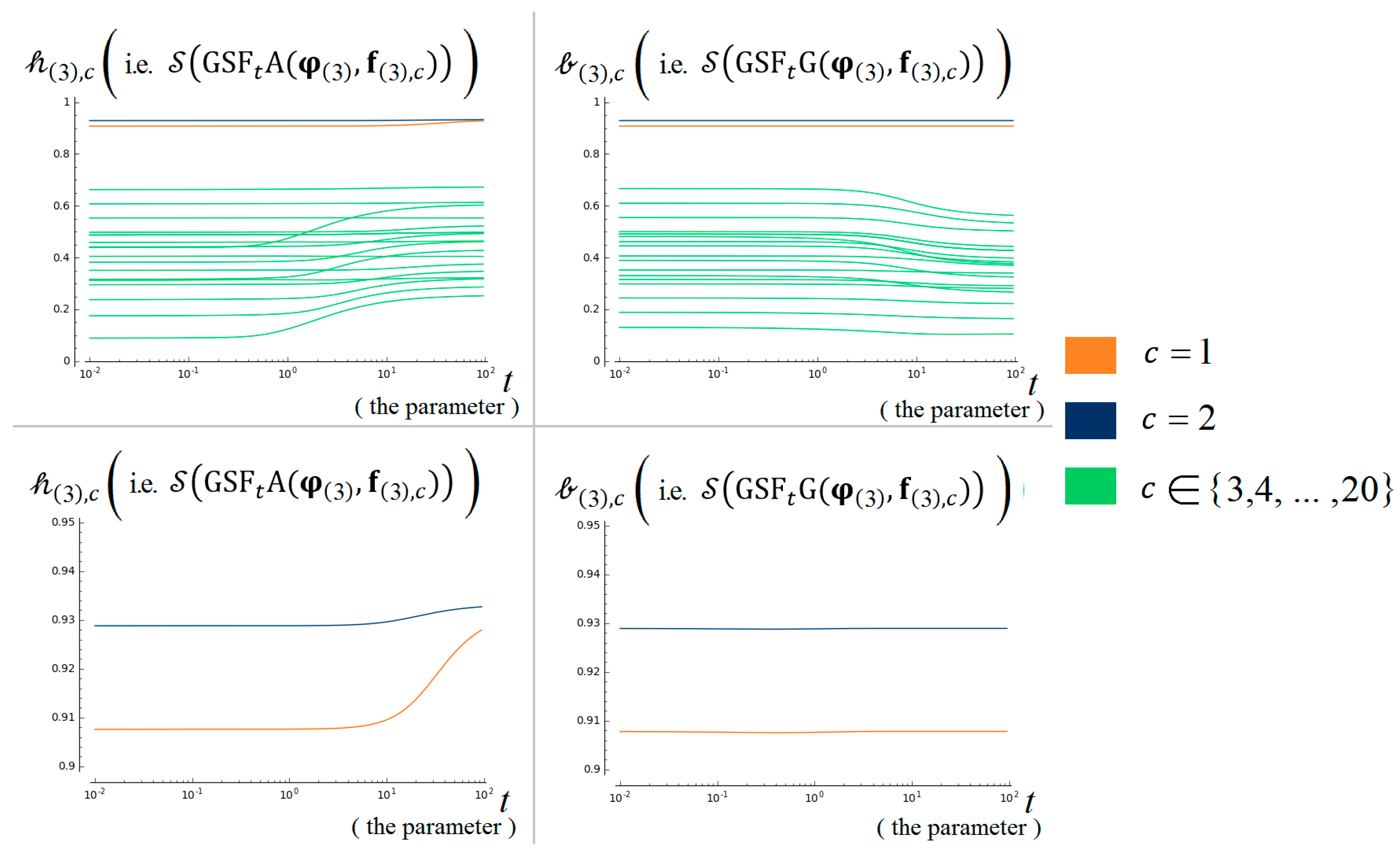
7.5. Test 4: t–Dependence Test

In the fourth test we are testing on the effectiveness of the choices of $t$ at influencing the sorting of the cities, for both ${\mathrm{GSF}}_t\mathrm{A}$ and ${\mathrm{GSF}}_t\mathrm{G}$.

7.5.1. t-Dependence Test of Type-A: For Environmental Management

The Test Inputs

There are 4 cities ${\mathfrak{A}}_{\left(4,\mathrm{A}\right)}=\left\{{\mathfrak{a}}_{\left(4,\mathrm{A}\right),1},{\mathfrak{a}}_{\left(4,\mathrm{A}\right),2},{\mathfrak{a}}_{\left(4,\mathrm{A}\right),3},{\mathfrak{a}}_{\left(4,\mathrm{A}\right),4}\right\}$ to be accessed during the interval of 10 days, ${\mathfrak{B}}_{\left(4,\mathrm{A}\right)}=\left\{{\mathfrak{b}}_{\left(4,\mathrm{A}\right),1},{\mathfrak{b}}_{\left(4,\mathrm{A}\right),2},\dots ,{\mathfrak{b}}_{\left(4,\mathrm{A}\right),10}\right\}$ for the severity of pollution on a given perception characterized by the value of $t$. For easier identification, ${\mathfrak{a}}_{\left(4,\mathrm{A}\right),1},{\mathfrak{a}}_{\left(4,\mathrm{A}\right),2},{\mathfrak{a}}_{\left(4,\mathrm{A}\right),3},{\mathfrak{a}}_{\left(4,\mathrm{A}\right),4}$ shall also be addressed as City $\mathrm{P},\mathrm{Q},\mathrm{R},\mathrm{S}$ respectively.

$$M_{\left(4,A\right)}=\left(\begin{array}{l}\langle 0.05,0.05,0.90\rangle \langle 0.05,0.05,0.90\rangle \langle 0.05,0.05,0.90\rangle \langle 0.99,0.01,0.01\rangle \langle 0.05,0.05,0.90\rangle \\ \langle 0.05,0.05,0.90\rangle \langle 0.05,0.05,0.90\rangle \langle 0.05,0.05,0.90\rangle \langle 0.05,0.05,0.90\rangle \langle 0.05,0.05,0.90\rangle \\ \\ \langle 0.99,0.01,0.01\rangle \langle 0.05,0.05,0.90\rangle \langle 0.05,0.05,0.90\rangle \langle 0.05,0.05,0.90\rangle \langle 0.05,0.05,0.90\rangle \\ \langle 0.05,0.05,0.90\rangle \langle 0.05,0.05,0.90\rangle \langle 0.05,0.05,0.90\rangle \langle 0.05,0.05,0.90\rangle \langle 0.05,0.05,0.90\rangle \\ \\ \langle 0.50,0.05,0.30\rangle \langle 0.50,0.05,0.30\rangle \langle 0.50,0.05,0.30\rangle \langle 0.10,0.05,0.52\rangle \langle 0.10,0.05,0.52\rangle \\ \langle 0.10,0.05,0.52\rangle \langle 0.10,0.05,0.52\rangle \langle 0.10,0.05,0.52\rangle \langle 0.10,0.05,0.52\rangle \langle 0.10,0.05,0.52\rangle \\ \\ \langle 0.30,0.10,0.40\rangle \langle 0.30,0.10,0.40\rangle \langle 0.30,0.10,0.40\rangle \langle 0.30,0.10,0.40\rangle \langle 0.30,0.10,0.40\rangle \\ \langle 0.30,0.10,0.40\rangle \langle 0.30,0.10,0.40\rangle \langle 0.30,0.10,0.40\rangle \langle 0.30,0.10,0.40\rangle \langle 0.30,0.10,0.40\rangle \end{array}\right)$$

$${\mathsf{\phi }}_{\left(4,\mathrm{A}\right)}=\left(0.100.100.100.100.100.100.100.100.100.10\right)$$

Denote $f_{(4,\mathrm{A}),c}$ = $c$-th row of $M_{(4,\mathrm{A})}$, ${𝓆}_c={\mathrm{GSF}}_t\mathrm{A}({\mathsf{\phi }}_{(4,\mathrm{A})},f_{(4,\mathrm{A}),c})$ for all $c$.

The Criteria of Compliance

There should exist $t_a,t_b,t_{c,1},t_{c,2}$, with ${10}^{-2}<t_a<t_b<t_{c,1}<{10}^2$ and $t_b<t_{c,2}<{10}^2$.

This is for the algorithm to yield:

• ${𝓆}_4\succcurlyeq {𝓆}_3\succcurlyeq {𝓆}_2$ and ${𝓆}_4\succcurlyeq {𝓆}_3\succcurlyeq {𝓆}_1$ whenever $t\in \left({10}^{-2},t_a\right)$
• ${𝓆}_3\succcurlyeq {𝓆}_4\succcurlyeq {𝓆}_2$ and ${𝓆}_3\succcurlyeq {𝓆}_4\succcurlyeq {𝓆}_1$ whenever $t\in \left(t_a,t_b\right)$
• ${𝓆}_3\succcurlyeq {𝓆}_1\succcurlyeq {𝓆}_4$ whenever $t\in \left(t_b,t_{c,1}\right)$
• ${𝓆}_3\succcurlyeq {𝓆}_2\succcurlyeq {𝓆}_4$ whenever $t\in \left(t_b,t_{c,2}\right)$
• ${𝓆}_1\succcurlyeq {𝓆}_3\succcurlyeq {𝓆}_4$ whenever $t\in \left(t_{c,1},{10}^2\right)$
• ${𝓆}_2\succcurlyeq {𝓆}_3\succcurlyeq {𝓆}_4$ whenever $t\in \left(t_{c,2},{10}^2\right)$

This is because:

• All the 10 days of City S are “slightly polluted”: $⟨0.30,0.10,0.40⟩$. Thus, the low values of $t$ should produce an “overview” or “generalizing” perception, where a general value or trend of the degree of pollution across all the days is of primary concern. This perception consequently results in the deduction of City S as the most polluted city, for low values of $t$.
• City P and City Q contains one day that is “severely polluted”: $⟨0.99,0.01,0.01⟩$. Thus, the high values of $t$ should produce a “pinpointing” perception, where the highest degree of pollution recorded on a particular day is of primary concern. This perception consequently results in the deduction of City P and City Q as the two most polluted cities, for high values of $t$.
  Remark 13:

  The most polluted city, out of City P and City Q depends on the objective weight which was already dealt by Test 3 from Section 7.4.
• City $\mathrm{R}$ contains three days that is “medially polluted”: $⟨0.50,0.05,0.30⟩$. Thus, the medium values of $t$ should produce a perception that is between “overview” and “pinpointing” in nature. This perception consequently results in the selection of City R as the most polluted city, for medium values of $t$.

The Results of Our Algorithm

Thus, it can be seen in Figure 7 that our algorithm ${\mathrm{GSF}}_t\mathrm{A}$ fully complies with the $t$-dependence test of type-A.

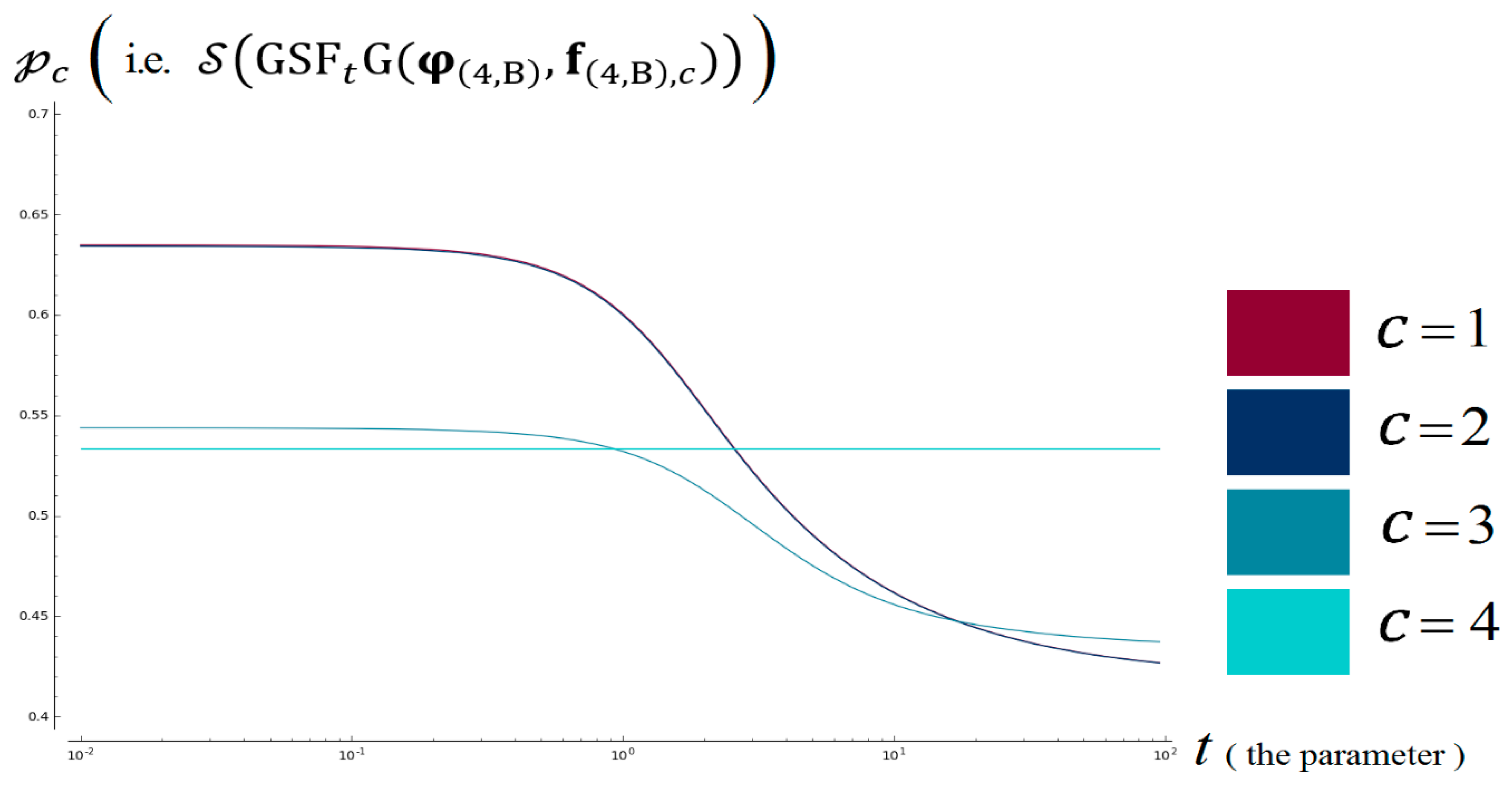
7.5.2. $t$-Dependence Test of Type-B: For Tourism Marketing

The Test Inputs

There are 4 cities ${\mathfrak{A}}_{\left(4,\mathrm{B}\right)}=\left\{{\mathfrak{a}}_{\left(4,\mathrm{B}\right),1},{\mathfrak{a}}_{\left(4,\mathrm{B}\right),2},{\mathfrak{a}}_{\left(4,\mathrm{B}\right),3},{\mathfrak{a}}_{\left(4,\mathrm{B}\right),4}\right\}$ to be accessed during the interval of 10 days, ${\mathfrak{B}}_{\left(4,\mathrm{B}\right)}=\left\{{\mathfrak{b}}_{\left(4,\mathrm{B}\right),1},{\mathfrak{b}}_{\left(4,\mathrm{B}\right),2},\dots ,{\mathfrak{b}}_{\left(4,\mathrm{B}\right),10}\right\}$ for the severity of pollution on a given perception characterized by the value of t. For easier identification, ${\mathfrak{a}}_{\left(4,\mathrm{B}\right),1},{\mathfrak{a}}_{\left(4,\mathrm{B}\right),2},{\mathfrak{a}}_{\left(4,\mathrm{B}\right),3},{\mathfrak{a}}_{\left(4,\mathrm{B}\right),4}$ shall also be addressed as City $\mathrm{T},\mathrm{U},\mathrm{V},\mathrm{W}$ respectively.

$$M_{\left(4,B\right)}=\left(\begin{array}{l}\langle 0.40,0.10,0.10\rangle \langle 0.40,0.10,0.10\rangle \langle 0.40,0.10,0.10\rangle \langle 0.40,0.10,0.10\rangle \langle 0.01,0.01,0.99\rangle \\ \langle 0.40,0.10,0.10\rangle \langle 0.40,0.10,0.10\rangle \langle 0.40,0.10,0.10\rangle \langle 0.40,0.10,0.10\rangle \langle 0.40,0.10,0.10\rangle \\ \\ \langle 0.40,0.10,0.10\rangle \langle 0.40,0.10,0.10\rangle \langle 0.40,0.10,0.10\rangle \langle 0.40,0.10,0.10\rangle \langle 0.40,0.10,0.10\rangle \\ \langle 0.01,0.01,0.99\rangle \langle 0.40,0.10,0.10\rangle \langle 0.40,0.10,0.10\rangle \langle 0.40,0.10,0.10\rangle \langle 0.40,0.10,0.10\rangle \\ \\ \langle 0.30,0.10,0.20\rangle \langle 0.30,0.10,0.20\rangle \langle 0.30,0.10,0.20\rangle \langle 0.30,0.10,0.20\rangle \langle 0.30,0.10,0.20\rangle \\ \langle 0.05,0.05,0.80\rangle \langle 0.05,0.05,0.80\rangle \langle 0.05,0.05,0.80\rangle \langle 0.30,0.10,0.20\rangle \langle 0.30,0.10,0.20\rangle \\ \\ \langle 0.20,0.10,0.40\rangle \langle 0.20,0.10,0.40\rangle \langle 0.20,0.10,0.50\rangle \langle 0.20,0.10,0.40\rangle \langle 0.20,0.10,0.40\rangle \\ \langle 0.20,0.10,0.40\rangle \langle 0.20,0.10,0.40\rangle \langle 0.20,0.10,0.40\rangle \langle 0.20,0.10,0.40\rangle \langle 0.20,0.10,0.40\rangle \end{array}\right)$$

$${\mathsf{\phi }}_{\left(4,\mathrm{B}\right)}=\left(0.100.100.100.100.100.100.100.100.100.10\right)$$

Denote $f_{\left(4,\mathrm{B}\right),c}$ = $c$-th row of $M_{\left(4,\mathrm{B}\right)}$, for all $c$, ${𝓅}_c={\mathrm{GSF}}_t\mathrm{G}({\mathsf{\phi }}_{\left(4,\mathrm{B}\right)},f_{\left(4,\mathrm{B}\right),c})$ for all $c$.

The Criteria of Compliance

There should exist ${10}^{-2}<t_a<t_b<t_c<t_d<t_e<{10}^2$.

There should exist $t_a,t_b,t_{c,1},t_{c,2}$ with ${10}^{-2}<t_a<t_b<t_{c,1}<{10}^2$ and $t_b<t_{c,2}<{10}^2$.

This is for the algorithm to yield:

• ${𝓅}_1\succcurlyeq {𝓅}_3\succcurlyeq {𝓅}_4$ and ${𝓅}_2\succcurlyeq {𝓅}_3\succcurlyeq {𝓅}_4$ whenever $t\in \left({10}^{-2},t_a\right)$.
• ${𝓅}_3\succcurlyeq {𝓅}_1\succcurlyeq {𝓅}_4$ and ${𝓅}_3\succcurlyeq {𝓅}_2\succcurlyeq {𝓅}_4$ whenever $t\in \left(t_a,t_b\right)$.
• ${𝓅}_3\succcurlyeq {𝓅}_4\succcurlyeq {𝓅}_1$ whenever $\in \left(t_b,t_{c,1}\right)$.
• ${𝓅}_3\succcurlyeq {𝓅}_4\succcurlyeq {𝓅}_2$ whenever $\in \left(t_b,t_{c,2}\right)$.
• ${𝓅}_4\succcurlyeq {𝓅}_3\succcurlyeq {𝓅}_1$ whenever $\in \left(t_{c,1},{10}^2\right)$.
• ${𝓅}_4\succcurlyeq {𝓅}_3\succcurlyeq {𝓅}_2$ whenever $\in \left(t_{c,2},{10}^2\right)$.

This is because:

• All the 10 days of City $\mathrm{W}$ are “slightly polluted”: $⟨0.20,0.10,0.40⟩$. Thus, the low values of $t$ should produce an “urgent” perception, where time is at stake and therefore the photographic team must quickly take photographs of a city. This perception consequently results in the deduction of City $\mathrm{W}$ as the least polluted city for low values of $t$.
• City $\mathrm{T}$ and City $\mathrm{U}$ contain one day that is “good”: $⟨0.01,0.01,0.99⟩$. Thus, the high values of $t$ should produce a “quality” perception, where the photographic team must wait for the clearest possible sky to produce the best possible photographs to market China tourism. This perception consequently results in the deduction of City $\mathrm{T}$ and City $\mathrm{U}$ as the two least polluted cities, for high values of $t$.
  Remark 14:

  The least polluted city, out of City $\mathrm{T}$ and City $\mathrm{U}$ depends on the objective weight which was already dealt by Test 3 from Section 7.4.
• City $\mathrm{V}$ contains three days that is “okay”: $⟨0.50,0.05,0.80⟩$. Thus, the medium values of $t$ should produce a perception that is between “urgent” and “quality” in nature. This perception consequently results in the deduction of City $\mathrm{V}$ as the least polluted city for medium values of $t$.

The Results of Our Algorithm

Thus, it can be seen in Figure 8 that our algorithm ${\mathrm{GSF}}_t\mathrm{G}$ fully complies with the $t$-dependence test of type-B.

It can be clearly observed that our algorithms comply with all of the tests that were outlined above, hence proving the accuracy of our algorithms and the corresponding formulas.

8. Conclusions

In this paper, we introduced two operators, namely, the generalized $t$-spherical fuzzy $w$-weighted geometric and arithmetic interaction functions. The structural properties of these operators were thoroughly studied and it was proven that the two newly introduced operators satisfy these properties. The highlight of this work is the development of two decision making algorithms based on these two operators, and the application of these algorithms in a multi-attribute multi-perception decision-making problem related to the ranking of the pollution level of five major Chinese cities. Further, we also presented a novel method to convert the values in the raw dataset into single-valued neutrosophic numbers, something which has not been done in existing literature. In addition to this, we have also outlined several tests to investigate the accuracy of the results yielded by our algorithm, and it was proven that our algorithm has demonstrated compliance with all of the tests that were outlined, thereby proving the accuracy of the results. Hence this work is definitely an important addition to the body of knowledge in this area of study.

References

- Zadeh, L.A. Information and control. Fuzzy Sets 1965, 8, 338–353. [Google Scholar]
- Atanassov, K.T. Intuitionistic fuzzy sets. Fuzzy Sets Syst. 1986, 20, 87–96. [Google Scholar] [CrossRef]
- Atanassov, K.T. Intuitionistic Fuzzy Sets; Springer-Verlag: Berlin/Heidelberg, Germany, 1999. [Google Scholar]
- Yager, R.R. Pythagorean fuzzy subsets. In Proceedings of the 2013 Joint IFSA World Congress and NAFIPS Annual Meeting (IFSA/NAFIPS), Edmonton, AB, Canada, 24–28 June 2013. [Google Scholar]
- Yager, R.R. Pythagorean membership grades in multi criteria decision making. IEEE Trans. Fuzzy Syst. 2014, 22, 958–965. [Google Scholar] [CrossRef]
- Yager, R.R. Generalized orthopair fuzzy sets. IEEE Trans. Fuzzy Syst. 2017, 25, 1222–1230. [Google Scholar] [CrossRef]
- Cuong, B.C. Picture Fuzzy Sets—First Results, Part 2; Tech. Rep; Institute of Mathematics, Vietnam Academy of Science and Technology: Hanoi, Vietnam, 2013. [Google Scholar]
- Cuong, B.C. Picture Fuzzy Sets—First Results, Part 1; Institute of Mathematics, Vietnam Academy of Science and Technology: Hanoi, Vietnam, 2013. [Google Scholar]
- Mahmood, T.; Ullah, K.; Khan, Q.; Jan, N. An approach toward decision-making and medical diagnosis problems using the concept of spherical fuzzy sets. Neural Comput. Appl. 2018, 1–13. [Google Scholar] [CrossRef]
- Xu, Z.S.; Yager, R.R. Some geometric aggregation operators based on intuitionistic fuzzy sets. Int. J. Gen. Syst. 2006, 35, 417–433. [Google Scholar] [CrossRef]
- Garg, H. Generalized intuitionistic fuzzy interactive geometric interaction operators using Einstein t-norm and t-conorm and their application to decision making. Comput. Ind. Eng. 2016, 101, 53–69. [Google Scholar] [CrossRef]
- Garg, H. Novel intuitionistic fuzzy decision making method based on an improved operation laws and its application. Eng. Appl. Artif. Intell. 2017, 60, 164–174. [Google Scholar] [CrossRef]
- He, Y.; Chen, H.; Zhau, L.; Liu, J.; Tao, Z. Intuitionistic fuzzy geometric interaction averaging operators and their application to multi-criteria decision making. Inf. Sci. 2014, 259, 142–159. [Google Scholar] [CrossRef]
- Zhao, X.; Wei, G. Some intuitionistic fuzzy Einstein hybrid aggregation operators and their application to multiple attribute decision making. Knowl. Based Syst. 2013, 37, 472–479. [Google Scholar] [CrossRef]
- Liu, P. Some frank aggregation operators for interval-valued intuitionistic fuzzy numbers and their application to group decision making. J. Mult. Valued Logic Soft Comput. 2017, 29, 183–223. [Google Scholar]
- Garg, H. A new generalized Pythagorean fuzzy information aggregation using Einstein operations and its application to decision making. Int. J. Intell. Syst. 2016, 31, 886–920. [Google Scholar] [CrossRef]
- Garg, H. Generalized Pythagorean fuzzy geometric interactive aggregation operators using Einstein operations and their application to decision making. J. Exp. Theor. Artif. Intell. 2018, 1–32. [Google Scholar] [CrossRef]
- Peng, X.; Dai, J.; Garg, H. Exponential operation and aggregation operator for q-rung orthopair fuzzy set and their decision-making method with a new score function. Int. J. Intell. Syst. 2018, 33, 2255–2282. [Google Scholar] [CrossRef]
- Wei, G. Picture fuzzy aggregation operators and their application to multiple attribute decision making. J. Intell. Fuzzy Syst. 2017, 33, 713–724. [Google Scholar] [CrossRef]
- Garg, H. Some picture fuzzy aggregation operators and their applications to multicriteria decision-making. Arab. J. Sci. Eng. 2017, 42, 5275–5290. [Google Scholar] [CrossRef]
- Garg, H.; Munir, M.; Ullah, K.; Mahmood, T.; Jan, N. Algorithm for T-Spherical Fuzzy Multi-Attribute Decision Making Based on Improved Interactive Aggregation Operators. Symmetry 2018, 10, 670. [Google Scholar] [CrossRef]
- Li, Y.; Deng, Y. Generalized ordered propositions fusion based on belief entropy. Int. J. Comp. Comm. Control 2018, 13, 792–807. [Google Scholar] [CrossRef]
- Fei, L.; Wang, H.; Chen, L.; Deng, Y. A new vector valued similarity measure for intuitionistic fuzzy sets based on OWA operators. Iran. J. Fuzzy Syst. 2019, 16, 113–126. [Google Scholar]
- Wang, W.; Liu, X. Interval-valued intuitionistic fuzzy hybrid weighted averaging operator based on Einstein operation and its application to decision making. J. Intell. Fuzzy Syst. 2013, 25, 279–290. [Google Scholar]
- Wang, W.; Liu, X. The multi-attribute decision making method based on interval-valued intuitionistic fuzzy Einstein hybrid weighted geometric operator. Comput. Math. Appl. 2013, 66, 1845–1856. [Google Scholar] [CrossRef]
- Wang, W.; Liu, X.; Qin, Y. Interval-valued intuitionistic fuzzy aggregation operators. J. Syst. Eng. Electron. 2012, 23, 574–580. [Google Scholar] [CrossRef]
- Xu, Z.S.; Xia, M. Induced generalized intuitionistic fuzzy operators. Knowl. Based Syst. 2003, 24, 197–209. [Google Scholar] [CrossRef]
- Garg, H.; Kumar, K. An advanced study on the similarity measures of intuitionistic fuzzy sets based on the set pair analysis theory and their application in decision making. Soft Comput. 2018, 22, 4959–4970. [Google Scholar] [CrossRef]
- Wei, G.-W.; Xu, X.-R.; Deng, D.-X. Interval-valued dual hesitant fuzzy linguistic geometric aggregation operators in multiple attribute decision making. Int. J. Knowl. Based Intell. Eng. Syst. 2016, 20, 189–196. [Google Scholar] [CrossRef] [Green Version]
- Garg, H. Some robust improved geometric aggregation operators under interval-valued intuitionistic fuzzy environment for multi-criteria decision-making process. J. Ind. Manag. Optim. 2018, 14, 283–308. [Google Scholar] [CrossRef] [Green Version]
- Chen, S.M.; Cheng, S.H.; Tsai, W.H. Multiple attribute group decision making based on interval-valued intuitionistic fuzzy aggregation operators and transformation techniques of interval—Valued intuitionistic fuzzy values. Inf. Sci. 2016, 367–368, 418–442. [Google Scholar] [CrossRef]
- Garg, H. Some arithmetic operations on the generalized sigmoidal fuzzy numbers and its application. Granul. Comput. 2018, 3, 9–25. [Google Scholar] [CrossRef]
- Chen, S.M.; Cheng, S.H.; Chiou, C.H. Fuzzy multiattribute group decision making based on intuitionistic fuzzy sets and evidential reasoning methodology. Inf. Fusion 2016, 27, 215–227. [Google Scholar] [CrossRef]
- Wei, G.W. Interval valued hesitant fuzzy uncertain linguistic aggregation operators in multiple attribute decision making. Int. J. Mach. Learn. Cybern. 2016, 7, 1093–1114. [Google Scholar] [CrossRef]
- Kumar, K.; Garg, H. Connection number of set pair analysis based TOPSIS method on intuitionistic fuzzy sets and their application to decision making. Appl. Intell. 2018, 48, 2112–2119. [Google Scholar] [CrossRef]
- Kumar, K.; Garg, H. Prioritized linguistic interval-valued aggregation operators and their applications in group decision-making problems. Mathematics 2018, 6, 209. [Google Scholar] [CrossRef]
- Khan, M.U.; Mahmood, T.; Ullah, K.; Jan, N.; Deli, I.; Khan, Q. Some aggregation operators for bipolar-valued hesitant fuzzy information based on Einstein operational laws. J. Eng. Appl. Sci. 2017, 36, 63–72. [Google Scholar]
- Garg, H. Some methods for strategic decision-making problems with immediate probabilities in Pythagorean fuzzy environment. Int. J. Intell. Syst. 2018, 33, 687–712. [Google Scholar] [CrossRef]
- Ullah, K.; Mahmood, T.; Jan, N. Similarity measures for t-spherical fuzzy sets with applications in pattern recognition. Symmetry 2018, 10, 193. [Google Scholar] [CrossRef]
- Garg, H. Linguistic Pythagorean fuzzy sets and its applications in multi attribute decision-making process. Int. J. Intell. Syst. 2018, 33, 1234–1263. [Google Scholar] [CrossRef]
- Garg, H. New logarithmic operational laws and their aggregation operators for Pythagorean fuzzy set and their applications. Int. J. Intell. Syst. 2018. [Google Scholar] [CrossRef]
- Garg, H.; Arora, R. Generalized and group-based generalized intuitionistic fuzzy soft sets with applications in decision-making. Appl. Intell. 2018, 48, 343–356. [Google Scholar] [CrossRef]
- Garg, H. New logarithmic operational laws and their applications to multiattribute decision making for single-valued neutrosophic numbers. Cogn. Syst. Res. 2018, 52, 931–946. [Google Scholar] [CrossRef] [Green Version]
- Rani, D.; Garg, H. Complex intuitionistic fuzzy power aggregation operators and their applications in multi-criteria decision-making. Expert Syst. 2018, e12325. [Google Scholar] [CrossRef]
- Ullah, K.; Mahmood, T.; Jan, N.; Broumi, S.; Khan, Q. On bipolar-valued hesitant fuzzy sets and their applications in multi-attribute decision making. Nucleus 2018, 55, 93–101. [Google Scholar]
- Selvachandran, G.; Quek, S.; Smarandache, F.; Broumi, S. An Extended Technique for Order Preference by Similarity to an Ideal Solution (TOPSIS) with Maximizing Deviation Method Based on Integrated Weight Measure for Single-Valued Neutrosophic Sets. Symmetry 2018, 10, 236. [Google Scholar] [CrossRef]
- Wang, H.; Smarandache, F.; Zhang, Y.Q.; Sunderraman, R. Single valued neutrosophic sets. Multispace Multistructure 2010, 4, 410–413. [Google Scholar]
- Nirmal, N.P.; Bhatt, M.G. Selection of automated guided vehicle using single valued neutrosophic entropy based on novel multi attribute decision making technique. New Trends Neutrosophic Theory Appl. 2016, 105–114. Available online: https://www.semanticscholar.org/paper/Selection-of-Automated-Guided-Vehicle-using-Single-ANGALBoomija/985a780ec046a90d1aec2895a89db53a8ae1a6d1 (accessed on 9 May 2019).
- Jha, S.; Kumar, R.; Priyadarshini, I.; Smarandache, F.; Long, H.V. Neutrosophic Image Segmentation with Dice Coefficients. Measurement 2019, 134, 762–772. [Google Scholar] [CrossRef]
- Nguyen, G.N.; Ashour, A.S.; Dey, N. A survey of the State-of-the-arts on Neutrosophic Sets in Biomedical Diagnoses. Int. J. Mach. Learn. Cybern. 2019, 10, 1–13. [Google Scholar] [CrossRef]
- Le Hoang, S.; Fujita, H. Neural-Fuzzy with Representative Sets for Prediction of Student Performance. Appl. Intell. 2019, 49, 172–187. [Google Scholar]
- Long, H.V.; Ali, M.; Khan, M.; Tu, D.N. A novel approach for Fuzzy Clustering based on Neutrosophic Association Matrix. Comput. Ind. Eng. 2019. [Google Scholar] [CrossRef]
- Kaur, S.; Bansal, R.K.; Mittal, M.; Goyal, L.M.; Kaur, I.; Verma, A. Mixed pixel decomposition based on extended fuzzy clustering for single spectral value remote sensing images. J. Indian Soc. Remote Sens. 2019, 47, 427–437. [Google Scholar] [CrossRef]
- Tuan, T.M.; Fujita, H.; Dey, N.; Ashour, A.S.; Ngoc, V.T.N.; Chu, D.T. Dental Diagnosis from X-Ray Images: An Expert System based on Fuzzy Computing. Biomed. Signal Process. Control 2018, 39C, 64–73. [Google Scholar]
- Ali, M.; Khan, M.; Tung, N.T. Segmentation of Dental X-ray Images in Medical Imaging using Neutrosophic Orthogonal Matrices. Expert Syst. Appl. 2018, 91, 434–441. [Google Scholar] [CrossRef]
- Ngan, R.T.; Ali, M. Delta-Equality of Intuitionistic Fuzzy Sets: A New Proximity Measure and Applications in Medical Diagnosis. Appl. Intell. 2018, 48, 499–525. [Google Scholar] [CrossRef]
- Ali, M.; Dat, L.Q.; Smarandache, F. Complex Neutrosophic Set: Formulation and Applications in Decision-Making. Int. J. Fuzzy Syst. 2018, 20, 986–999. [Google Scholar] [CrossRef]
- Giap, C.N.; Son, L.H.; Chiclana, F. Dynamic Structural Neural Network. J. Intell. Fuzzy Syst. 2018, 34, 2479–2490. [Google Scholar] [CrossRef]
- Ngan, R.T.; Cuong, B.C.; Ali, M. H-max distance measure of intuitionistic fuzzy sets in decision making. Appl. Soft Comput. 2018, 69, 393–425. [Google Scholar] [CrossRef]
- Le, T.; Le Son, H.; Vo, M.; Lee, M.; Baik, S. Cluster-Based Boosting Algorithm for Bankruptcy Prediction in a Highly Imbalanced Dataset. Symmetry 2018, 10, 250. [Google Scholar] [CrossRef]
- Khan, M.; Son, L.; Ali, M.; Chau, H.; Na, N.; Smarandache, F. Systematic Review of Decision Making Algorithms in Extended Neutrosophic Sets. Symmetry 2018, 10, 314. [Google Scholar] [CrossRef]
- Hemanth, D.J.; Anitha, J.; Mittal, M. Diabetic Retinopathy Diagnosis from Retinal Images using Modified Hopfield Neural Network. J. Med. Syst. 2018, 42, 247–253. [Google Scholar] [CrossRef]
- Ngan, T.T.; Lan, L.T.H.; Ali, M.; Tamir, D.; Son, L.H.; Tuan, T.M.; Rishe, N.; Kandel, A. Logic Connectives of Complex Fuzzy Sets. Rom. J. Inf. Sci. Technol. 2018, 21, 344–358. [Google Scholar]
- Jain, R.; Jain, N.; Kapania, S.; Son, L. Degree Approximation-Based Fuzzy Partitioning Algorithm and Applications in Wheat Production Prediction. Symmetry 2018, 10, 768. [Google Scholar] [CrossRef]
- Hemanth, D.J.; Anitha, J.; Naaji, A.; Geman, O.; Popescu, D.E. Modified Deep Convolutional Neural Network for Abnormal Brain Image Classification. IEEE Access 2018, 7, 4275–4283. [Google Scholar] [CrossRef]
- Phong, P.H.; Son, L.H. Linguistic Vector Similarity Measures and Applications to Linguistic Information Classification. Int. J. Intell. Syst. 2017, 32, 67–81. [Google Scholar] [CrossRef]
- Son, L.H.; Thong, P.H. Some Novel Hybrid Forecast Methods Based On Picture Fuzzy Clustering for Weather Nowcasting from Satellite Image Sequences. Appl. Intell. 2017, 46, 1–15. [Google Scholar] [CrossRef]
- Son, L.H.; Tuan, T.M. Dental segmentation from X-ray images using semi-supervised fuzzy clustering with spatial constraints. Eng. Appl. Artif. Intell. 2017, 59, 186–195. [Google Scholar] [CrossRef]
- Hai, D.T.; Le Vinh, T. Novel Fuzzy Clustering Scheme for 3D Wireless Sensor Networks. App. Soft Comput. 2017, 54, 141–149. [Google Scholar] [CrossRef]
- Son, L.H. Measuring Analogousness in Picture Fuzzy Sets: From Picture Distance Measures to Picture Association Measures. Fuzzy Optim. Decis. Mak. 2017, 16, 359–378. [Google Scholar] [CrossRef]
- Thanh, N.D.; Ali, M.; Son, L.H. A Novel Clustering Algorithm in a Neutrosophic Recommender System for Medical Diagnosis. Cognit. Comput. 2017, 9, 526–544. [Google Scholar] [CrossRef]
- Son, L.H.; Tien, N.D. Tune up Fuzzy C-Means for Big Data: Some novel hybrid clustering algorithms based on Initial Selection and Incremental Clustering. Int. J. Fuzzy Syst. 2017, 19, 1585–1602. [Google Scholar] [CrossRef]
- Son, L.H.; Tuan, T.M. A cooperative semi-supervised fuzzy clustering framework for dental X-ray image segmentation. Expert Syst. Appl. 2016, 46, 380–393. [Google Scholar] [CrossRef]
- Wijayanto, A.W.; Purwarianti, A.; Son, L.H. Fuzzy geographically weighted clustering using artificial bee colony: An efficient geo-demographic analysis algorithm and applications to the analysis of crime behavior in population. Appl. Intell. 2016, 44, 377–398. [Google Scholar] [CrossRef]
- Thong, P.H.; Son, L.H. Picture Fuzzy Clustering: A New Computational Intelligence Method. Soft Comput. 2016, 20, 3549–3562. [Google Scholar] [CrossRef]
- Son, L.J.; Hai, P.V. A novel multiple fuzzy clustering method based on internal clustering validation measures with gradient descent. Int. J. Fuzzy Syst. 2016, 18, 894–903. [Google Scholar] [CrossRef]
- Tuan, T.M.; Ngan, T.T.; Son, L.H. A Novel Semi-Supervised Fuzzy Clustering Method based on Interactive Fuzzy Satisficing for Dental X-Ray Image Segmentation. Appl. Intell. 2016, 45, 402–428. [Google Scholar] [CrossRef]
- Son, L.H.; Phong, P.H. On the performance evaluation of intuitionistic vector similarity measures for medical diagnosis. J. Intell. Fuzzy Syst. 2016, 31, 1597–1608. [Google Scholar] [CrossRef]
- Son, L.H. Generalized Picture Distance Measure and Applications to Picture Fuzzy Clustering. Appl. Soft Comput. 2016, 46, 284–295. [Google Scholar] [CrossRef]
- Thong, P.H.; Son, L.H. A Novel Automatic Picture Fuzzy Clustering Method Based On Particle Swarm Optimization and Picture Composite Cardinality. Knowl. Based Syst. 2016, 109, 48–60. [Google Scholar] [CrossRef]
- Thong, P.H.; Son, L.H. Picture Fuzzy Clustering for Complex Data. Eng. Appl. Artif. Intell. 2016, 56, 121–130. [Google Scholar] [CrossRef]
- Ngan, T.T.; Tuan, T.M.; Minh, N.H.; Dey, N. Decision making based on fuzzy aggregation operators for medical diagnosis from dental X-ray images. J. Med. Syst. 2016, 40, 1–7. [Google Scholar] [CrossRef] [PubMed]
- Son, L.H. DPFCM: A Novel Distributed Picture Fuzzy Clustering Method on Picture Fuzzy Sets. Expert Syst. Appl. 2016, 42, 51–66. [Google Scholar] [CrossRef]