Improved Compact Cuckoo Search Algorithm Applied to Location of Drone Logistics Hub


College of Computer Science and Engineering, Shandong University of Science and Technology, Qingdao 266590, China
*
Author to whom correspondence should be addressed.
Mathematics 2020, 8(3), 333; https://doi.org/10.3390/math8030333
Submission received: 31 January 2020
/
Revised: 26 February 2020
/
Accepted: 27 February 2020
/
Published: 3 March 2020
(This article belongs to the Special Issue Supply Chain Optimization)
Abstract
:Drone logistics can play an important role in logistics at the end of the supply chain and special environmental logistics. At present, drone logistics is in the initial development stage, and the location of drone logistics hubs is an important issue in the optimization of logistics systems. This paper implements a compact cuckoo search algorithm with mixed uniform sampling technology, and, for the problem of weak search ability of the algorithm, this paper combines the method of recording the key positions of the search process and increasing the number of generated solutions to achieve further improvements, as well as implements the improved compact cuckoo search algorithm. Then, this paper uses 28 test functions to verify the algorithm. Aiming at the problem of the location of drone logistics hubs in remote areas or rural areas, this paper establishes a simple model that considers the traffic around the village, the size of the village, and other factors. It is suitable for selecting the location of the logistics hub in advance, reducing the cost of drone logistics, and accelerating the large-scale application of drone logistics. This paper uses the proposed algorithm for testing, and the test results indicate that the proposed algorithm has strong competitiveness in the proposed model.
1. Introduction
There are many complex optimization scenarios in the fields of industry, finance, mathematics, etc. Some of them are difficult to find a true global optimal solution. The meta-heuristic algorithm is suitable for dealing with problems that are not solved by specific effective methods [1,2,3,4]. The Cuckoo Search (CS) algorithm is a new heuristic algorithm that simulates cuckoo parasitic brooding and solves complex optimization problems [5,6]. The CS uses the nest position of the cuckoo bird to represent a possible solution in the solution space. The cuckoo bird’s parasitic brooding behavior is used to search the solution space of the complex optimization problem. The movement of the solution is realized by the cuckoo’s Levy flight mechanism, and the potential better solution is found through continuous searching and updating. The Levy flight mechanism used in the cuckoo algorithm can effectively jump out of the local optimal solution, and thus has better global search performance. It has also achieved better results in engineering optimization problems [6,7]. Since the cuckoo algorithm was proposed, various improved versions of the algorithm have been proposed for different uses, such as Modified Cuckoo Search (MCS) [8], Binary Cuckoo Search (BCS) [9], Multiobjective Cuckoo Search (MOCS) [10], Chaotic Cuckoo Search (CCS) [11], etc. This type of algorithm is usually used to solve complex optimization problems, thus it will set a population to obtain better solutions in a shorter time. Therefore, when dealing with complex optimization problems, or when it is applied to a device with limited memory, the heuristic algorithm needs to be improved to achieve the same or better solution in a shorter time or with less memory consumption.
Compact is a technique that can reduce the memory usage of the meta-heuristic algorithm. By using a probabilistic model to replace the population used in the algorithm from a macro perspective, it achieves less memory usage and shorter calculation time [12,13,14,15,16,17,18]. The compact method uses a probability model to represent the original population, and then uses the probability model to generate a new solution. By comparing the generated solutions, the probability model is updated, which is then used to replace the population update in the original algorithm [12]. Some related algorithm improvements using the compact method have been proposed, such as compact particle swarm optimization (cPSO) [12], compact genetic algorithm (cGA) [13], compact differential evolution (cDE) [14], compact bat algorithm (cBA) [15], etc. This article attempts to implement an improved version of the compact CS algorithm with a mixture of normal and uniform distributions. For the problem of weak search ability of the algorithm, this paper combines the method of recording the key positions of the search process and increasing the number of generated solutions to achieve further improvements and implements the improved compact cuckoo search algorithm (icCS). The algorithm was tested using 28 test functions of CEC2017.
As a new logistics method in the supply chain, drone logistics can effectively improve the efficiency of the logistics system and solve the problem of express delivery in the last mile of the current logistics system [19,20]. Drone logistics, with its own advantages, can perform express delivery in rural, mountainous, or congested areas, as well as areas where ground traffic is impassable [20]. It can also be used in special situations and applied to scenarios that require rapid delivery, such as medical rescue and blood product transportation [21,22,23,24]. To apply drones to logistics systems, there have been many related studies. In addition to optimizing the design of logistics systems and logistics drones [25], it is also necessary to design logistics models based on cost, efficiency, and other factors. Flight optimization in the process of logistics distribution of drones is also an issue that needs to be researched in the field of drone logistics [26]. There are currently two main models of drone logistics: models for distribution centers and drones and those for delivery vehicles and drones. Many scholars have studied the logistics mode of combining drone and truck transportation [27,28]. For the model of using truck transportation and drone for distribution, the logistics problem is usually regarded as a path planning problem with the drone [29]. Then, usually the travelling salesman problem is used to solve it on the basis of adding drones [30]. Intelligent algorithms are also applied to such problems [31]. In addition, there are many studies using machine learning to deal with supply chain problems. Some machine learning methods, such as Bayesian optimization, can also effectively deal with optimization problems [32,33]. The logistics mode of distribution centers and drones usually focuses on the location of the logistics center, and, because of the low load of the drone itself and the limited battery energy, the logistics of the drone are limited [34]. In addition, other scholars have studied other influencing factors of drone logistics, including operating costs, differences between urban and rural areas, etc. [35,36].
Hu et al. [37] used CS to deal with the trajectory planning of micro aerial vehicles for express transportation in cities. Considering the wind field, the obstacles of the building, and the characteristics of the goods, the cuckoo algorithm is used to plan the transportation path. This paper focuses on rural and remote areas, where surrounding villages are served by setting up a drone logistics hub. The path of the drone during transportation is a straight line between the logistics hub and the village. The main problem is the optimization of the location of the logistics hub. This paper aims at the logistics scenarios in rural and remote areas, using the logistics model of distribution centers and drones, assuming that future logistics drones can or have a stronger load capacity and longer dwell time. Then, the location of the drone logistics hub is simply modeled and tested using the algorithm proposed in this paper.
2. Related Work
This section briefly introduces the cuckoo search algorithm and the drone logistics hub location model proposed in this paper.
2.1. Metaheuristics Algorithm of Cuckoo
The CS algorithm is a new meta-heuristic algorithm that simulates the breeding strategy of cuckoo in nature [5]. It solves complex optimization problems by imitating the brooding and parasitic behavior of cuckoos in nature. The cuckoo search algorithm uses the position of the bird nest to represent a possible solution, and updates the solution by updating the position of the bird nest. The update method uses Lévy flight to simulate the movement pattern of birds in nature. Lévy flight consists of long-range flights with occasional large steps and short-range flights with frequent small steps. The occasional long-distance flight in Lévy flight can expand the search range and prevent falling into local optimum.
To simplify the implementation of this algorithm, three simple and idealized rules are set for the cuckoo search algorithm. (1) Each cuckoo produces only one egg at a time, and then randomly selects a location for hatching. (2) The nest with the best eggs will be preserved and passed on to the next generation. (3) The number of nests that can be used is fixed, and the probability of the eggs in the nest being found is . When the egg is found, the owner of the nest will throwaway the egg or build a new nest. The cuckoo search algorithm uses the parameter to control local search and global exploration [38]. The formula for local search is written as
where represents the next generation solution, i is a cuckoo in the solution, is the step size, is a Heaviside function, is a random number generated by a uniform distribution, and and represent two randomly selected different solutions from all current possible solutions. The implementation formula for global exploration is written as
In Equation (2), indicates the step size scaling factor, usually . The random step size in Lévy flight is generated using the Lévy probability distribution.
The variance and mean of the distribution are infinite. According to the original literature of the CS algorithm [5], the pseudo-code of the algorithm is shown in Algorithm 1.

2.2. Location Model of Drone Logistics Hub
At present, drone logistics is limited by the low load and weak endurance of drones. Moreover, drones have limited mobility and cannot perform long-term continuous delivery, thus the current more reasonable model is the collaborative model of delivery vehicles and drones. Then, path planning for delivery vehicles and drones is performed. However, after the drone picks up the goods from the delivery vehicle for delivery, it is necessary to consider that the drone returns to the delivery vehicle after the recipient receives it. The movement of the delivery vehicle and the uncertainty of the recipient’s pickup time will significantly reduce the drone’s delivery efficiency. However, with the development of technology, drone equipment for logistics will solve the current problems, and, when the level of automation increases, the mode of combining small unmanned logistics centers with drones will become more competitive.
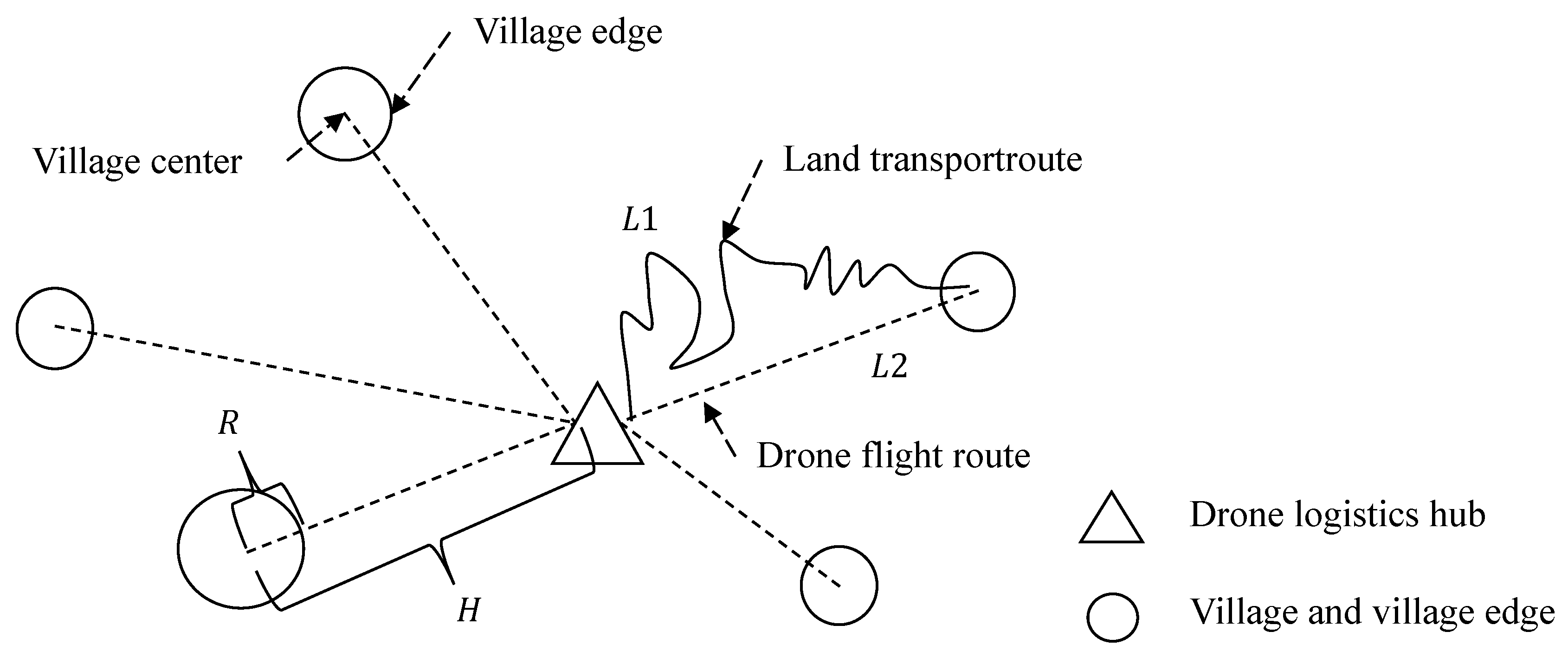
This paper chooses the model of unmanned logistics center and drone, and applies it to the location of unmanned logistics hub in rural areas. The simulation diagram of the model in two-dimensional space is shown in Figure 1. The premise assumptions and explanations of the model are as follows:
- (1)
- The frone only travels to and from one village at a time.
- (2)
- The drone’s endurance is able to meet the flight requirements from the logistics hub to the farthest village that the logistics hub is responsible for.
- (3)
- Under ideal conditions, the drone distribution path is a straight line from the logistics hub to the corresponding village.
- (4)
- Each logistics hub is responsible for express delivery services in multiple villages, and each village chooses the nearest logistics hub to serve it.
- (5)
- The sizes of the villages are different, that is, the areas of the villages and the numbers of villagers are different.
- (6)
- Drones do not enter the village when delivering goods, but deliver goods to the edge of the village to ensure safety.
- (7)
- The land transportation distance from the logistics hub to each village is different and the degree of traffic difficulty is measured by the distance.
- (8)
- The number of logistics hubs is artificially set according to the scope of application and artificially selected after calculating different solutions.
The circle in Figure 1 represents the village, and the size of the circle represents the radius of the village, which is expressed as R. The triangle represents the drone logistics station, and H represents the straight line distance between the logistics hub and the village center. The model established in this paper is relatively simple. This paper only considers the distribution distance, the size of the village, and the current village’s efficiency ratio of using drone logistics to land transportation, which is used to indicate the degree of difficulty of land transportation. The objective function of the model is written as
In the formula, represents the straight line distance from the center of the village labeled i to the nearest logistics hub. is the distance between a village and a logistics hub minus the village radius, as drone delivery is not delivered to the precise location of the recipient, but is delivered to the edge of the village, which can ensure better security. N is the total number of villages to be considered. is the number of people living in the village. The larger is the population, the more frequently does the logistics center deliver to the village, thus the logistics hub needs to be closer to the village to reduce the overall cost. is the distance for land transportation, is the distance for linear delivery using drones, and is usually a value greater than 1, thus the logistics hub needs to be closer to villages with high land distribution costs. The variables and parameters involved in the model can be obtained through actual measurement. There are no unnatural parameters, and the degree of traffic difficulty is also obtained by using land transportation distance and straight flight distance. All parameters can be calculated from the application environment data during actual application.The solution obtained after calculating the model is the relative positions of multiple logistics hubs, and different villages choose their nearest logistics hubs based on the distance. In the end, different solutions will be generated according to the number of logistics hubs. Because the proposed model does not take into account all the influencing factors, and the importance of the model’s constraints is different in different situations, it needs to be artificially selected according to actual conditions.
3. Improved Compact Cuckoo Search Algorithm
This section introduces the application of the compact scheme and improved compact scheme to cuckoo search algorithm.
3.1. Compact Scheme
The essence of the distribution estimation algorithm (EDA) is to use the probability model to represent the population in the meta-heuristic algorithm, use the probability model to represent the population from a macro perspective, and implement the operation on the population in the meta-heuristic algorithm by operating the probability model [42,43]. The compact method is an effective method to reduce the memory footprint of the meta-heuristic algorithm. By updating the probability model instead of updating the entire population, the calculation amount is reduced and the algorithm running time is shortened.
Firstly, the probabilistic model is constructed using the original population distribution, and then the population is updated by evaluating the probability model to find the optimal solution. Since the probability model is used to represent the entire population, the characteristics of the original population are described from a macro perspective. Perturbation Vector (PV) is often used to represent the characteristics of the entire population. PV is constantly changing with the operation of the algorithm, which is defined as: , where is used to representing the mean value of the PV, is the standard deviation of the PV, and t is used to represent the number of current iterations. Each pair of mean and standard deviation corresponds to a probability density function (PDF), which is truncated at and normalized to an area of amplitude of 1 [44]. Using the PV vector, the solution can be randomly generated by the inverse cumulative distribution function (CDF). After generating two solutions using PV, usually which is better is judged by comparing the fitness function values of the two solutions; the better solution is the and the worse solution is the . Then, the PV is updated. The formula for updating each standard deviation and the average value in the PV using and is as follows:
where represents the newly generated average and is the virtual population. The update rules for are as follows:
The PV vector and the generated individual solution are stored during algorithm execution, instead of storing the location of the entire population solution and the motion vector, which achieves less runtime memory usage and is beneficial for use on resource-constrained devices. However, since the conventional compact algorithm only randomly generates one solution at a time, there are fewer possible solutions explored during each iteration, which will cause the problem of insufficient convergence ability in the later iterations, and the method needs to be improved.
3.2. Improved Compact Scheme
The compact algorithm saves more memory resources, reduces the amount of calculation, and shortens the algorithm running time compared with the original algorithm. However, the compact algorithm generates two solutions per iteration and compares them. The solution generated during each iteration is less than the population-based method in the original algorithm. Therefore, the number of overall searches is small, the algorithm will converge slowly in the later stages of iteration, and it is easy to fall into a local optimum.
Because the compact algorithm uses PV to generate new solutions, with continuous iteration, PV will slowly converge to a certain area, but the number of solutions generated by PV during each iteration is small, thus it is difficult to jump out of the local optimum. Thus, the method of sampling using the normal distribution in the compact mode is improved. Considering the above problems, this paper chooses to add the uniform distribution sampling method on the basis of using the original compact mode. As shown in Algorithm 2, a new solution is generated using PV during each iteration, and another new solution is generated using uniform sampling. Then, CS is used to update the two generated solutions. Using uniform sampling in the solution space can search for other regions to find a better solution while the PV converges to the optimal region. Because there may be better solutions around the solution generated during the iteration, to get closer to the surrounding better solution during the iteration, a perturbation operation on the optimal value is added in this paper, as shown in Algorithm 2.
| Algorithm 2: Improved compact cuckoo search algorithm. |
 |
After improving the compact mode, the algorithm can achieve better results and convergence ability, but the global search ability and local search ability can still be further improved. Therefore, a switching mode is added in this paper. When the algorithm is trapped in a local optimal value, it switches to a population-based search mode, as shown in Algorithm 2. There are many ways to judge when the algorithm is trapped in a local optimal value. The first method can compare the recent iteration trend with the overall iteration trend. The second method can determine whether a better solution can be found within a certain number of iterations. This paper uses the second method to switch modes. The possible solutions when the mode is switched are divided into two parts, one is selected from the optimal solution obtained during the execution of the compact algorithm, and the other is generated using a uniform distribution, as shown in Algorithm 2, where n is the number of new solutions generated per iteration after switching.
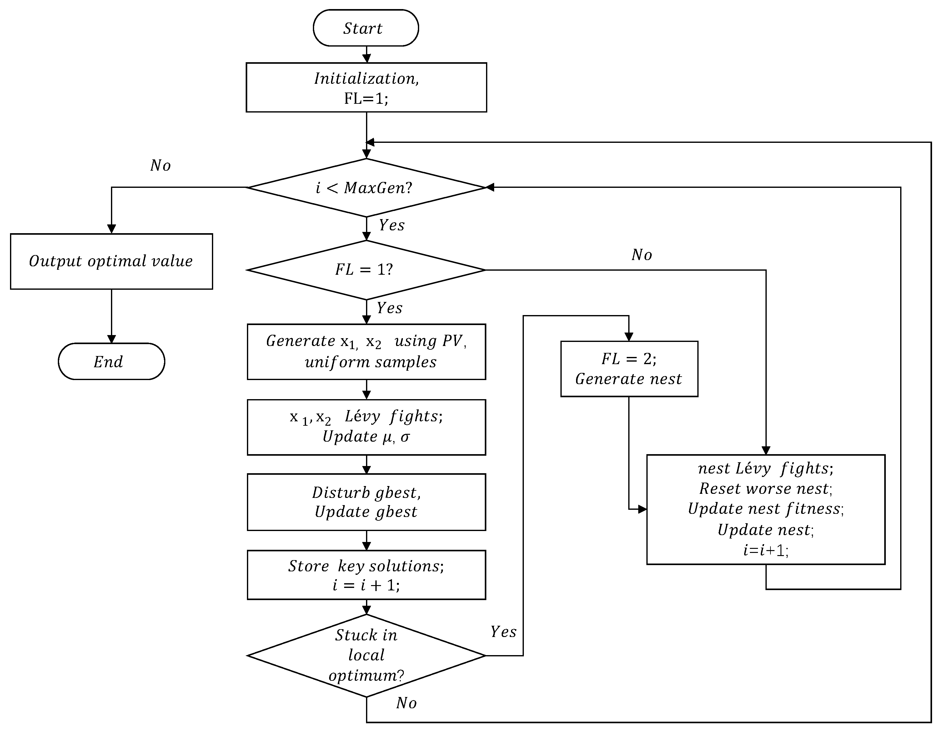
There are many ways to obtain the optimal solution from the operation of the compact algorithm. This article chooses the key solution of the optimal solution in the previous iterative process. The selection of the key solution needs to conform to Equation (7); the difference between the fitness function value of the key solution and the previous solution is greater than the difference of the first m optimal values of the key solution. m in this paper is 20. t represents the current number of iterations and is used to store the optimal solution obtained during each iteration. By selecting the key solution from the optimal solution for each iteration, it is possible to use the previous search results for a more refined search, which is a memory-based approach. Selecting those breakthrough solutions in the iterative process through Equation (7) can assist in fine search after switching. Based on the above introduction, the flow chart of the icCS algorithm in this paper is given in Figure 2.
4. Experimental Results
The proposed algorithm was tested. The test function used CEC’17 benchmark suite [45]. The 28 test functions used in this study include unimodal functions, simple multimodal functions, mixed functions, and composition functions. All test functions used are minimization problems and are defined as follows:
where D is the number of dimensions and the search range is . According to the introduction of CEC’17 benchmark suite, was excluded because it exhibits unstable behavior, especially for higher dimensions in test functions. Compared with the same algorithm implemented in Matlab, the performance of the one implemented in C is very different [45]. Thus, 28 test functions were used to the the algorithm in this paper. All tested algorithms maintained consistent parameter settings. The population size of all algorithms was 20 and the number of algorithm iterations was set to 3000. Each algorithm was tested five times on each function and the average value was retained. The parameter settings of each comparison algorithm are shown in Table 1.
4.1. Comparison with Common Optimization Algorithms
The improved compact cuckoo search algorithm proposed in this paper was compared with common classical algorithms on the test functions: the original CS algorithm [5]; the Adaptive Cuckoo Search Algorithm (ACS) [46], in which the parameter was set to 0.25; common PSO [47]; DE [48]; and the sine cosine algorithm (SCA) proposed in 2016 [49]. The comparison results are shown in Table 2.
Table 2 shows the average value obtained by running the icCS algorithm and other algorithms on the test functions. The last row in the table summarizes the comparison results of icCS algorithm and other algorithms, where w indicates on how many test functions icCS has achieved better results than the algorithm results of the current column. Table 3 shows the standard deviation of the icCS algorithm and other algorithms on the test functions.
According to the data in Table 2 and Table 3, the algorithm proposed in this paper achieved better results than other algorithms on the test functions. Especially on specific functions, such as , , and , compared with CS and ACS algorithms, the proposed algorithm could obtain better and more stable results. At the same time, the overall performance of each algorithm compared with the icCS algorithm was measured at a significant level = 0.05 under the Wilcoxon’s sign rank test (Table 4) [50].
According to Table 2, compared with CS, icCS achieved better or similar results on 19 functions; compared with ACS, icCS achieved better or similar results on 17 functions; compared with the PSO algorithm, icCS obtained better or similar results on 15 functions, with better results than PSO on functions , , , , , , and ; and compared with DE, icCS achieved better or similar results on 16 functions, obtaining better results on functions , , , , , , . However, DE could find the global optimal value effectively on and , which was better than other algorithms. Compared with SCA, icCS achieved better or similar results on all functions. For the comparison of standard deviations, Table 3 gives the corresponding data. Combined with the data in Table 2, the icCS algorithm proposed in this paper has similar stability compared with CS and ACS algorithms. However, the CS and ACS algorithms on , , and did not achieve good results. Based on the above comparison, the overall performance of the algorithm icCS proposed in this paper is better on 28 test functions.
4.2. Comparison with Compact Algorithms
Table 5 and Table 6 compare the proposed pcCS algorithm with other common algorithms using the compact method, including compact Particle Swarm Optimization (cPSO) [12], compact Bat Algorithm (cBA) [15], and compact Artificial Bee Colony algorithms (cABC) [51]. The number of virtual populations was set to 20 and the parameters of the algorithm remained the same as those in the original document.
This paper compares the proposed icCS algorithm with other compact algorithms in 10D and 30D optimization. At the same time, the overall performance of each other algorithm was measured at a significant level = 0.05 under Wilcoxon sign rank test. According to the data in Table 5 and Table 6, the algorithm proposed in this paper has better performance than the other three compact algorithms and can obtain better results. For the cBA algorithm in Table 5, icCS achieved better results on , , , , , , , and . Combined with the results of Wilcoxon sign rank test, the proposed icCS algorithm was significantly better than the cBA algorithm on 28 test functions. For the cPSO and cABC algorithms, the cABC algorithm could still obtain better results when it was optimized in 10D, but, when it was optimized in 30D, as shown in Table 6, the cABC algorithm was not as stable as the proposed icCS algorithm. As shown in Table 5 for 10D optimization and Table 6 for 30D optimization, the performance of the proposed icCS algorithm in different dimensions is similar and does not fluctuate too much. According to the results of the Wilcoxon sign rank test, the proposed icCS algorithm was significantly better than other algorithms using only compact technology for the 28 test functions and both 10D and 30D optimization.
4.3. Convergence Evaluation
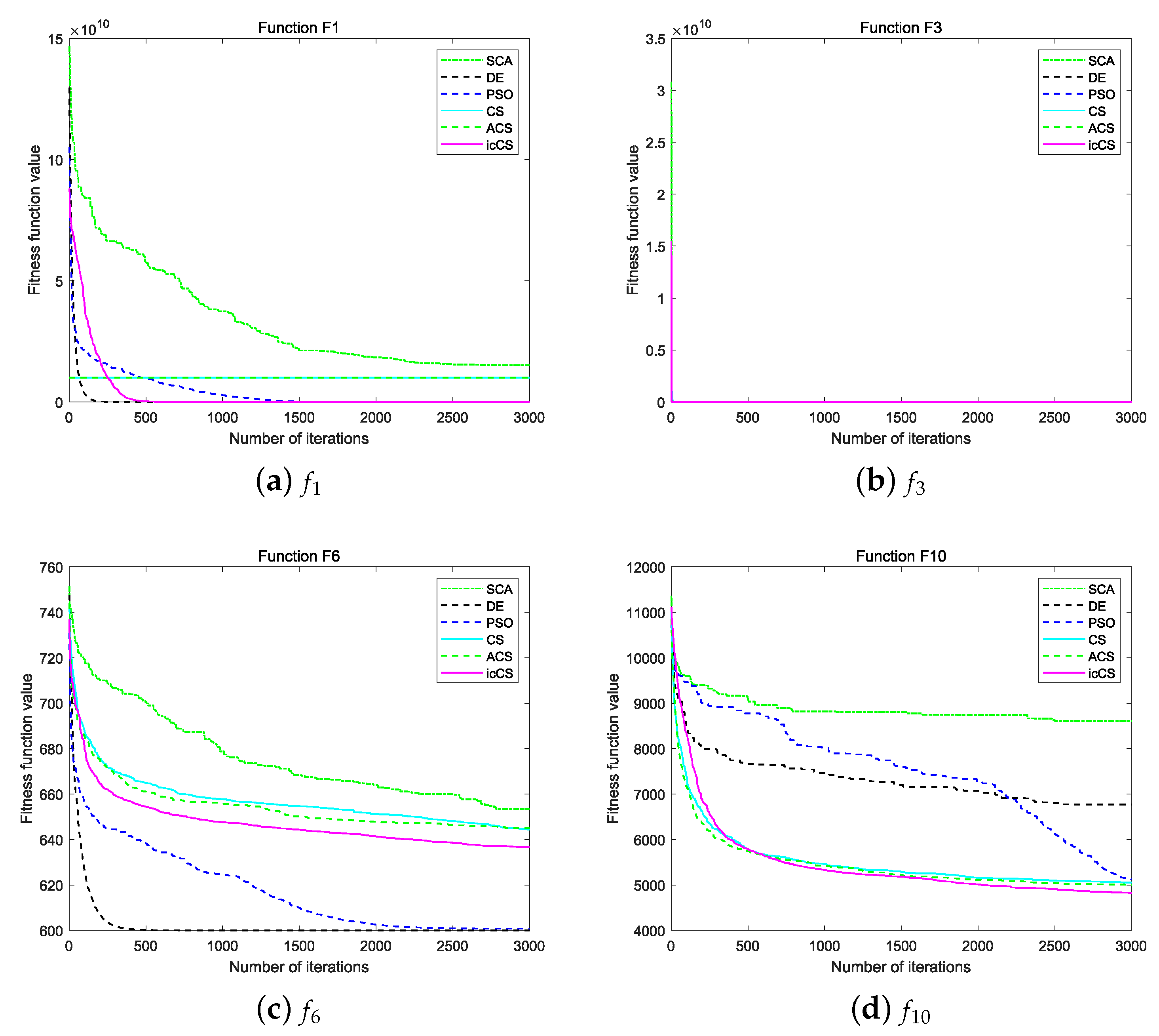
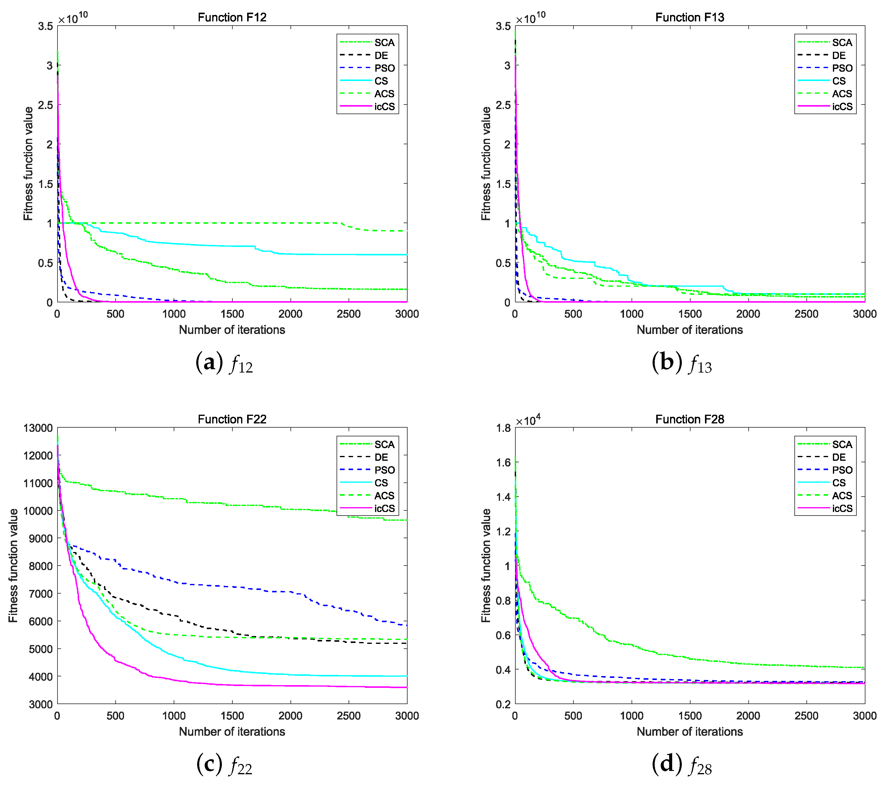
The optimal value obtained by the algorithm cannot completely define the validity of the algorithm’s search principle. It is also necessary to evaluate the convergence of the algorithm to measure the speed of the algorithm reaching the optimal value. In this study, two unimodal functions (), two simple multimodal functions (), two hybrid functions (), and two composition functions () were selected as the test functions to compare the convergence of icCS and other common classic algorithms for evaluation of convergence. The comparison of the convergence performance of the icCS algorithm proposed in this paper and other common classical algorithms is shown in Figure 3 and Figure 4.
Because the algorithm proposed in this paper combines compact- and population-based technologies, the overall complexity of the algorithm is higher than that of algorithms using only compact. Based on the introduction of the algorithm in Section 3, the proposed icCS algorithm is divided into two phases. The first stage uses compact technology. To increase the global search capability at this stage, a step of uniform sampling is added in this paper. Sn additional uniform distribution sampling is performed on the basis of compact using normal distribution sampling. In this way, a new solution is generated during each iteration and two new solutions are generated, which increases the global search capability and also increases the complexity of the algorithm. At the same time, because the compact method generates fewer solutions, as shown in Figure 3 and Figure 4, the early convergence speed of the proposed algorithm is slow.
After the algorithm switches to the second stage, the algorithm uses a population-based method for enhanced search in order to jump out of the local optimum. The algorithm complexity at this time is the same as the original population-based algorithm. In addition, during the execution of the first phase of the algorithm, it is necessary to prepare for switching to the second phase. The key solutions in the first phase need to be saved, and it is necessary to judge whether to switch to the second phase continuously. Therefore, the overall complexity of the algorithm is similar to or slightly higher than the original algorithm.
5. Application to Drone Logistics Hub Location
The location of the drone logistics hub is briefly introduced in Section 2.2, which establishes a simple model based on three influencing factors, and then determines the fitness function of the model. In this section, the proposed algorithm is applied to the model for testing.
In fact, there are many studies on the way of drone logistics. The endurance time and load capacity of the drone itself also limit the development of drone logistics. However, there are studies on the innovative design of drone applications in the logistics industry [25]. With the development of technology, the restrictions on drone logistics due to the lack of performance of the drone itself will be gradually resolved. Thus, this paper focuses on the logistics issues in rural areas and remote mountain areas, and uses a model of logistics hubs and drones. A certain number of unmanned logistics hubs is used to provide logistics distribution services for surrounding villages and drones complete the end logistics tasks.
According to the above model and the introduction in Section 2.2, this article considers three factors that affect the location of the logistics center: the distance from the village to its logistics hub, the rural population, and the degree of transportation difficulty from the logistics hub to the village. The significance of the first factor is that the total distance between the logistics hub and the villages it serves is the smallest, and its operating costs are also smaller. The significance of the second factor is that, if the rural population is larger, the frequency of services required is higher, thus the proportion of the village in the whole is higher. Then, the logistics hub needs to be closer to the village, thus the cost is lower and the logistics efficiency will be higher. The significance of the third factor lies in the advantage of the drone’s straight flight. Traditional land logistics methods need to consider terrain factors, and roads are not straight, thus logistics in remote areas or mountain regions is more difficult. By adding this factor, logistics hubs can provide better logistics services to areas with difficult transportation. Based on the above and the introduction in Section 2.2, the objective function used in this paper is written as
where k is the kth village, is the population of villages k, N is the total number of villages, is the radius of the village, and is the straight line distance from the village to the nearest logistics hub to the village. The meaning of is the same as , and is the land transportation distance from the current village to the nearest logistics hub. The goal of the intelligent algorithm is to find the best logistics hub location so that the objective function is the smallest overall. That is, is minimized in Equation (10) by an intelligent algorithm to achieve the overall minimum, where is the position of the drone logistics hub in a certain dimension.
A program was used to generate the original test data based on the proposed drone logistics hub location model. Thirty random village locations were generated in a two-dimensional space of 50,000 m × 50,000 m. The radii of the villages were 200–900 m and their populations were 300–3000. The degree of traffic difficulty was the land transportation distance divided by the drone’s straight flight distance, which ranged from 1 to 3. Two generated models were used for testing. Table 7 shows the results of testing using Model 1. N is the number of logistics hubs for 30 villages. Each test was executed 50 times and the number of iterations was 3000. Table 8 shows the data results of the test using Model 2. N is the number of logistics hubs for 30 villages. Each test was performed 30 times and the number of iterations was 5000.
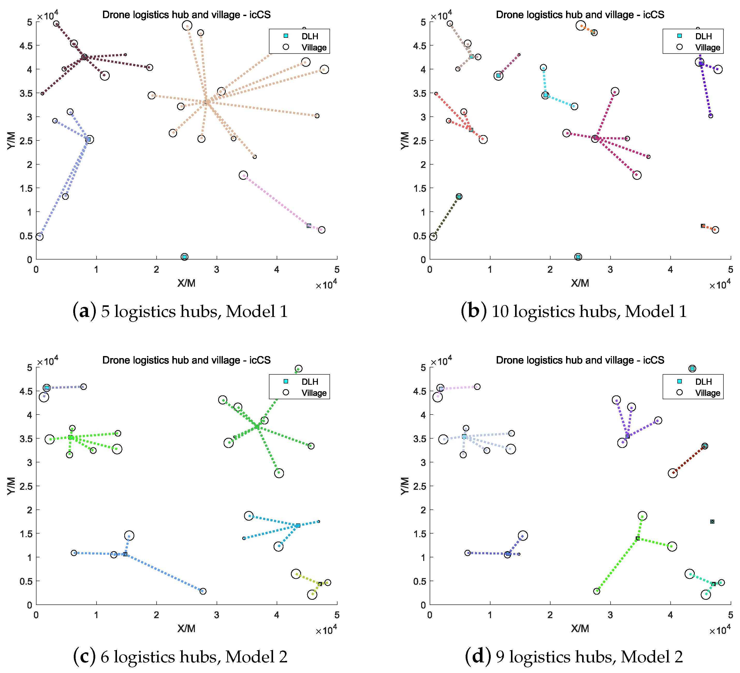
Figure 5 shows the results of running different models using different algorithms, where circles represent the village location, squares represent the calculated logistics hub location, and circles of different sizes represent villages with different radii. According to the execution result data, setting more logistics hubs can obtain smaller fitness function values. However, the construction of the logistics hub itself also requires costs. The larger is the number of logistics hubs, the higher is the overall cost, and the more dispersed are the goods, thus it is necessary to set an appropriate number of logistics hubs based on actual needs. It can be seen in Figure 5 that the location of some logistics hubs has been transferred to the village area after calculation, which means that the cost of logistics hubs will also be reduced, thus they can be selected based on actual conditions.
6. Conclusions and Discussion
Drone logistics will play an increasingly important role in the logistics industry with the increase in the degree of automation of the supply chain. This paper presents a simple location model for a drone logistics hub. This model considers three factors that affect location selection and determines the fitness function of the model. This paper is based on the original cuckoo search algorithm, which is improved by compact and other technology, and proposes the icCS algorithm. On the basis of sampling using the normal distribution, uniform distribution sampling and optimal solution perturbation are added, and, for the problem that is easy to fall into a local optimum, the global search ability is improved by increasing the number of generated solutions. Then, this paper uses the proposed algorithm to calculate the location for drone logistics hub. Compared with other algorithms, it can get better execution results. However, the model proposed in this paper is still inadequate, the influencing factors included are not comprehensive enough, and further improvements can be made, such as adding logistics hub cost, topographical influence, path planning between logistics hubs, and communication and control between logistics hub and drone. The proposed approach may be further improved by adopting some intelligent and efficient algorithms.
Author Contributions
Conceptualization, P.-C.S. and J.-S.P.; formal analysis, J.-S.P., P.-C.S., and S.-C.C.; Methodology, J.-S.P., P.-C.S., S.-C.C., and Y.-J.P.; validation, J.-S.P.; writing—original draft preparation, P.-C.S.; and writing—review and editing, J.-S.P., P.-C.S., S.-C.C., and Y.-J.P. All authors have read and agreed to the published version of the manuscript.
Funding
This research received no external funding.
Conflicts of Interest
The authors declare no conflict of interest.
References
- BoussaïD, I.; Lepagnot, J.; Siarry, P. A survey on optimization metaheuristics. Inf. Sci. 2013, 237, 82–117. [Google Scholar] [CrossRef]
- Pan, J.S.; Hu, P.; Chu, S.C. Novel Parallel Heterogeneous Meta-Heuristic and Its Communication Strategies for the Prediction of Wind Power. Processes 2019, 7, 845. [Google Scholar] [CrossRef] [Green Version]
- Du, Z.G.; Pan, J.S.; Chu, S.C.; Luo, H.J.; Hu, P. Quasi-Affine Transformation Evolutionary Algorithm With Communication Schemes for Application of RSSI in Wireless Sensor Networks. IEEE Access 2020, 8, 8583–8594. [Google Scholar] [CrossRef]
- Wang, J.; Ju, C.; Gao, Y.; Sangaiah, A.K.; Kim, G.J. A PSO based energy efficient coverage control algorithm for wireless sensor networks. Comput. Mater. Contin. 2018, 56, 433–446. [Google Scholar]
- Yang, X.S.; Deb, S. Cuckoo Search via Lévy flights. In Proceedings of the IEEE 2009 World Congress on Nature Biologically Inspired Computing (NaBIC), Coimbatore, India, 9–11 December 2009; pp. 210–214. [Google Scholar] [CrossRef]
- Yang, X.S.; Deb, S. Engineering Optimisation by Cuckoo Search. arXiv 2010, arXiv:1005.2908. [Google Scholar] [CrossRef]
- Gandomi, A.H.; Yang, X.S.; Alavi, A.H. Cuckoo search algorithm: A metaheuristic approach to solve structural optimization problems. Eng. Comput. 2013, 29, 17–35. [Google Scholar] [CrossRef]
- Walton, S.; Hassan, O.; Morgan, K.; Brown, M. Modified cuckoo search: A new gradient free optimisation algorithm. Chaos Sol. Fract. 2011, 44, 710–718. [Google Scholar] [CrossRef]
- Rodrigues, D.; Pereira, L.A.; Almeida, T.; Papa, J.P.; Souza, A.; Ramos, C.C.; Yang, X.S. BCS: A binary cuckoo search algorithm for feature selection. In Proceedings of the IEEE 2013 IEEE International Symposium on Circuits and Systems (ISCAS), Beijing, China, 19–23 May 2013; pp. 465–468. [Google Scholar]
- Yang, X.S.; Deb, S. Multiobjective cuckoo search for design optimization. Comput. Oper. Res. 2013, 40, 1616–1624. [Google Scholar] [CrossRef]
- Wang, G.G.; Deb, S.; Gandomi, A.H.; Zhang, Z.; Alavi, A.H. Chaotic cuckoo search. Soft Comput. 2016, 20, 3349–3362. [Google Scholar] [CrossRef]
- Neri, F.; Mininno, E.; Iacca, G. Compact Particle Swarm Optimization. Inf. Sci. 2013, 239, 96–121. [Google Scholar] [CrossRef]
- Harik, G.R.; Lobo, F.G.; Goldberg, D.E. The compact genetic algorithm. IEEE Trans. Evol. Comput. 1999, 3, 287–297. [Google Scholar] [CrossRef] [Green Version]
- Mininno, E.; Neri, F.; Cupertino, F.; Naso, D. Compact differential evolution. IEEE Trans. Evol. Comput. 2010, 15, 32–54. [Google Scholar] [CrossRef]
- Nguyen, T.T.; Pan, J.S.; Dao, T.K. A Compact Bat Algorithm for Unequal Clustering in Wireless Sensor Networks. Appl. Sci. 2019, 9, 1973. [Google Scholar] [CrossRef] [Green Version]
- Xue, X.; Pan, J.S. A Compact Co-Evolutionary Algorithm for sensor ontology meta-matching. Knowl. Inf. Syst. 2018, 56, 335–353. [Google Scholar] [CrossRef]
- Nguyen, T.T.; Pan, J.S.; Dao, T.K. An Improved Flower Pollination Algorithm for Optimizing Layouts of Nodes in Wireless Sensor Network. IEEE Access 2019, 7, 75985–75998. [Google Scholar] [CrossRef]
- Tian, A.Q.; Chu, S.C.; Pan, J.S.; Cui, H.; Zheng, W.M. A Compact Pigeon-Inspired Optimization for Maximum Short-Term Generation Mode in Cascade Hydroelectric Power Station. Sustainability 2020, 12, 767. [Google Scholar] [CrossRef] [Green Version]
- Yildirim, Z.G. New Approaches in Supply Chains: A Research on the Use of Drone Technology in Logistics. J. Strateg. Res. Soc. Sci. 2016, 2, 133–142. [Google Scholar]
- Rabta, B.; Wankmüller, C.; Reiner, G. A drone fleet model for last-mile distribution in disaster relief operations. Int. J. Disaster Risk Reduct. 2018, 28, 107–112. [Google Scholar] [CrossRef]
- Scott, J.; Scott, C. Drone delivery models for healthcare. Proc. Int. Conf. Syst. Sci. 2017, 3297–3304. [Google Scholar] [CrossRef] [Green Version]
- Amukele, T.; Ness, P.M.; Tobian, A.A.R.; Boyd, J.; Street, J. Drone transportation of blood products. Transfusion 2017, 57, 582–588. [Google Scholar] [CrossRef]
- Ling, G.; Draghic, N. Aerial drones for blood delivery. Transfusion 2019, 59, 1608–1611. [Google Scholar] [CrossRef] [PubMed] [Green Version]
- Amukele, T.K.; Hernandez, J.; Snozek, C.L.; Wyatt, R.G.; Douglas, M.; Amini, R.; Street, J. Drone transport of chemistry and hematology samples over long distances. Am. J. Clin. Pathol. 2017, 148, 427–435. [Google Scholar] [CrossRef] [PubMed] [Green Version]
- Kornatowski, P.M.; Bhaskaran, A.; Heitz, G.M.; Mintchev, S.; Floreano, D. Last-centimeter personal drone delivery: Field deployment and user interaction. IEEE Robot. Autom. Lett. 2018, 3, 3813–3820. [Google Scholar] [CrossRef]
- Hartjes, S.; van Hellenberg Hubar, M.E.G.; Visser, H.G. Multiple-phase trajectory optimization for formation flight in civil aviation. CEAS Aeronaut. J. 2019, 10, 453–462. [Google Scholar] [CrossRef] [Green Version]
- Murray, C.C.; Chu, A.G. The flying sidekick traveling salesman problem: Optimization of drone-assisted parcel delivery. Transp. Res. Part C Emerg. Technol. 2015, 54, 86–109. [Google Scholar] [CrossRef]
- Carlsson, J.G.; Song, S. Coordinated logistics with a truck and a drone. Manag. Sci. 2018, 64, 4052–4069. [Google Scholar] [CrossRef] [Green Version]
- Wang, D.; Hu, P.; Du, J.; Zhou, P.; Deng, T.; Hu, M. Routing and scheduling for hybrid truck-drone collaborative parcel delivery with independent and truck-carried drones. IEEE Internet Things J. 2019, 6, 10483–10495. [Google Scholar] [CrossRef]
- Agatz, N.; Bouman, P.; Schmidt, M. Optimization approaches for the traveling salesman problem with drone. Transp. Sci. 2018, 52, 965–981. [Google Scholar] [CrossRef]
- Ha, Q.M.; Deville, Y.; Pham, Q.D.; Hà, M.H. A hybrid genetic algorithm for the traveling salesman problem with drone. J. Heurist. 2019, 26, 219–2479. [Google Scholar] [CrossRef] [Green Version]
- Imani, M.; Ghoreishi, S.F. Bayesian optimization objective-based experimental design. In Proceedings of the IEEE 2020 American Control Conference (ACC 2020), Denver, CO, USA, 3 July 2020. [Google Scholar]
- Ghoreishi, S.F.; Imani, M. Bayesian optimization for efficient design of uncertain coupled multidisciplinary systems. In Proceedings of the IEEE 2020 American Control Conference (ACC 2020), Denver, CO, USA, 3 July 2020. [Google Scholar]
- Kim, S.; Moon, I. Traveling salesman problem with a drone station. IEEE Trans. Syst. Man Cybern. Syst. 2018, 49, 42–52. [Google Scholar] [CrossRef]
- Sudbury, A.W.; Hutchinson, E.B. A cost analysis of amazon prime air (drone delivery). J. Econ. Educ. 2016, 16, 1–12. [Google Scholar]
- Park, J.; Kim, S.; Suh, K. A comparative analysis of the environmental benefits of drone-based delivery services in urban and rural areas. Sustainability 2018, 10, 888. [Google Scholar] [CrossRef] [Green Version]
- Hu, H.; Wu, Y.; Xu, J.; Sun, Q. Cuckoo search-based method for trajectory planning of quadrotor in an urban environment. Proc. Inst. Mech. Eng. Part G J. Aerosp. Eng. 2019, 233, 4571–4582. [Google Scholar] [CrossRef]
- Yang, X.S.; Deb, S. Cuckoo search: Recent advances and applications. Neural Comput. Appl. 2014, 24, 169–174. [Google Scholar] [CrossRef] [Green Version]
- Clerc, M.; Kennedy, J. The particle swarm-explosion, stability, and convergence in a multidimensional complex space. IEEE Trans. Evol. Comput. 2002, 6, 58–73. [Google Scholar] [CrossRef] [Green Version]
- Jiang, M.; Luo, Y.P.; Yang, S.Y. Stochastic convergence analysis and parameter selection of the standard particle swarm optimization algorithm. Inf. Process. Lett. 2007, 102, 8–16. [Google Scholar] [CrossRef]
- Wang, F.; He, X.; Wang, Y.; Yang, S. Markov model and convergence analysis based on cuckoo search algorithm. Comput. Eng. 2012, 38, 180–185. [Google Scholar]
- Larrañaga, P.; Lozano, J.A. Estimation of Distribution Algorithms: A New Tool For Evolutionary Computation; Springer Science & Business Media: Berlin/Heidelberg, Germany, 2001; Volume 2. [Google Scholar]
- Chu, S.C.; Xue, X.; Pan, J.S.; Wu, X. Optimizing ontology alignment in vector space. J. Internet Technol. 2020, 21, 15–22. [Google Scholar]
- Bronshtein, I.N.; Semendyayev, K.A. Handbook of Mathematics; Springer Science & Business Media: Berlin/Heidelberg, Germany, 2013. [Google Scholar]
- Awad, N.; Ali, M.; Liang, J.; Qu, B.; Suganthan, P. Problem Definitions and Evaluation Criteria for the Cec 2017 Special Session and Competition on Single Objective Real-Parameter; Nanyang Technological University, Singapore, Tech. Rep.: Nanyang, China, 2016. [Google Scholar]
- Naik, M.; Nath, M.R.; Wunnava, A.; Sahany, S.; Panda, R. A new adaptive Cuckoo search algorithm. In Proceedings of the IEEE 2015 IEEE 2nd International Conference on Recent Trends in Information Systems (ReTIS), Kolkata, India, 9–11 July 2015; pp. 1–5. [Google Scholar]
- Kennedy, J.; Eberhart, R. Particle swarm optimization. In Proceedings of the IEEE ICNN’95-International Conference on Neural Networks, Perth, WA, Australia, 27 November–1 December 1995; Volume 4, pp. 1942–1948. [Google Scholar]
- Price, K.; Storn, R.M.; Lampinen, J.A. Differential Evolution: A Practical Approach to Global Optimization; Springer Science & Business Media: Berlin/Heidelberg, Germany, 2006. [Google Scholar]
- Mirjalili, S. SCA: A Sine Cosine Algorithm for solving optimization problems. Knowl.-Based Syst. 2016, 96, 120–133. [Google Scholar] [CrossRef]
- Woolson, R.F. Wilcoxon Signed-Rank Test. Wiley Encycl. Clin. Trials 2008, 1–3. [Google Scholar] [CrossRef]
- Dao, T.K.; Pan, T.S.; Nguyen, T.T.; Chu, S.C. A Compact Articial Bee Colony Optimization for Topology Control Scheme in Wireless Sensor Networks. J. Netw. Intell. 2015, 6, 297–310. [Google Scholar]
Figure 1.
Location model of drone logistics hub.

Figure 2.
The overall flow chart of icCS.

Figure 3.
Convergence test results for functions ,,, and in 30 dimensions: (a) ; (b) ; (c) ; and (d) .
Figure 3.
Convergence test results for functions ,,, and in 30 dimensions: (a) ; (b) ; (c) ; and (d) .

Figure 4.
Convergence test results for functions , , , and in 30 dimensions: (a) ; (b) ; (c) ; and (d) .
Figure 4.
Convergence test results for functions , , , and in 30 dimensions: (a) ; (b) ; (c) ; and (d) .

Figure 5.
Execution results of drone logistics hub location problem under different models and different numbers of hubs: (a) five logistics hubs, Model 1; (b) ten logistics hubs, Model 1; (c) six logistics hubs, Model 2; and (d) nine logistics hubs, Model 2.
Figure 5.
Execution results of drone logistics hub location problem under different models and different numbers of hubs: (a) five logistics hubs, Model 1; (b) ten logistics hubs, Model 1; (c) six logistics hubs, Model 2; and (d) nine logistics hubs, Model 2.


Table 1.
Parameters setting of each algorithm.
| Algorithm | Main Parameters Setting |
|---|---|
| CS | Population_number = 20, Max_iteration = 3000, Pa = 0.25 |
| ACS | Population_number = 20, Max_iteration = 3000, Pa = 0.25 |
| PSO | Population_number = 20, Max_iteration = 3000, = 0.9, = 0.4, c1 = 2, c2 = 2 |
| DE | Population_number = 20, Max_iteration = 3000, pCR = 0.2, Fmin = 0.2, Fmax = 0.8 |
| SCA | Population_number = 20, Max_iteration = 3000 |
| icCS | Population_number = 20, Max_iteration = 3000, Pa = 0.25 |
| cPSO | Population_number = 20, Max_iteration = 3000, = 1, = 1.5, = 2, c1 = 1, c2 = 1 |
| cBA | Population_number = 20, Max_iteration = 3000, loudness = 0.5, pulse rate = 0.5, min/max frequency = [0,2] |
| cABC | Population_number = 20, Max_iteration = 3000, limit = 100 |
Table 2.
Comparison of means of fitness functions on 30D optimization among CS, ACS, PSO, DE, SCA, and icCS is presented here.
Table 2.
Comparison of means of fitness functions on 30D optimization among CS, ACS, PSO, DE, SCA, and icCS is presented here.
| Functions | icCS | CS | ACS | PSO | DE | SCA |
|---|---|---|---|---|---|---|
| 1.20377 × 10 | 1.00000 × 10 | 1.00000 × 10 | 4.56091 × 10 | 3.18520 × 10 | 1.51701 × 10 | |
| 3.05501 × 10 | 3.79292 × 10 | 3.22087 × 10 | 1.70774 × 10 | 8.66524 × 10 | 5.75645 × 10 | |
| 4.62444 × 10 | 4.73280 × 10 | 4.65491 × 10 | 5.40339 × 10 | 4.92410 × 10 | 1.93646 × 10 | |
| 6.76672 × 10 | 6.68839 × 10 | 6.34201 × 10 | 5.62882 × 10 | 6.36734 × 10 | 8.00897 × 10 | |
| 6.36546 × 10 | 6.44382 × 10 | 6.44924 × 10 | 6.00733 × 10 | 6.00000 × 10 | 6.53341 × 10 | |
| 9.50101 × 10 | 9.35106 × 10 | 9.64459 × 10 | 8.26945 × 10 | 8.72143 × 10 | 1.18146 × 10 | |
| 9.42849 × 10 | 9.40035 × 10 | 9.23222 × 10 | 8.65031 × 10 | 9.36081 × 10 | 1.07358 × 10 | |
| 5.07394 × 10 | 5.64605 × 10 | 9.30145 × 10 | 1.16805 × 10 | 9.00000 × 10 | 6.44206 × 10 | |
| 4.82195 × 10 | 5.05056 × 10 | 4.99931 × 10 | 5.12150 × 10 | 6.76785 × 10 | 8.60907 × 10 | |
| 1.22792 × 10 | 1.21607 × 10 | 1.20667 × 10 | 1.24541 × 10 | 1.20299 × 10 | 2.57068 × 10 | |
| 4.56905 × 10 | 6.00015 × 10 | 9.00368 × 10 | 6.21396 × 10 | 4.15010 × 10 | 1.61706 × 10 | |
| 1.81192 × 10 | 1.00001 × 10 | 1.00001 × 10 | 1.80866 × 10 | 1.77057 × 10 | 6.63131 × 10 | |
| 1.48212 × 10 | 1.47295 × 10 | 1.48013 × 10 | 4.06132 × 10 | 9.25870 × 10 | 2.99047 × 10 | |
| 1.62982 × 10 | 1.61110 × 10 | 1.63020 × 10 | 1.64717 × 10 | 5.03273 × 10 | 2.12505 × 10 | |
| 2.60602 × 10 | 2.65977 × 10 | 2.69191 × 10 | 2.22859 × 10 | 2.45510 × 10 | 3.82109 × 10 | |
| 2.04739 × 10 | 2.07413 × 10 | 2.01007 × 10 | 2.03341 × 10 | 1.93289 × 10 | 2.59000 × 10 | |
| 7.44420 × 10 | 7.67991 × 10 | 8.73722 × 10 | 1.25873 × 10 | 9.36373 × 10 | 4.69351 × 10 | |
| 1.94031 × 10 | 1.94203 × 10 | 1.95316 × 10 | 1.29213 × 10 | 2.77813 × 10 | 4.60719 × 10 | |
| 2.39270 × 10 | 2.43996 × 10 | 2.45306 × 10 | 2.23193 × 10 | 2.20637 × 10 | 2.84076 × 10 | |
| 2.44515 × 10 | 2.44476 × 10 | 2.41188 × 10 | 2.36641 × 10 | 2.44690 × 10 | 2.57886 × 10 | |
| 3.59559 × 10 | 4.00541 × 10 | 5.33379 × 10 | 5.83669 × 10 | 5.18629 × 10 | 9.64492 × 10 | |
| 2.81251 × 10 | 2.82287 × 10 | 2.77342 × 10 | 2.72533 × 10 | 2.78211 × 10 | 3.05061 × 10 | |
| 2.95136 × 10 | 2.99155 × 10 | 2.92443 × 10 | 2.92132 × 10 | 2.99210 × 10 | 3.21214 × 10 | |
| 2.88699 × 10 | 2.88668 × 10 | 2.88775 × 10 | 2.90573 × 10 | 2.88754 × 10 | 3.27954 × 10 | |
| 4.10369 × 10 | 4.71619 × 10 | 3.80533 × 10 | 4.42989 × 10 | 4.95267 × 10 | 7.52475 × 10 | |
| 3.22191 × 10 | 3.22988 × 10 | 3.22089 × 10 | 3.25043 × 10 | 3.21313 × 10 | 3.46664 × 10 | |
| 3.18150 × 10 | 3.17620 × 10 | 3.16887 × 10 | 3.27739 × 10 | 3.23058 × 10 | 4.11323 × 10 | |
| 3.82243 × 10 | 3.88243 × 10 | 3.93256 × 10 | 3.65520 × 10 | 3.71836 × 10 | 4.93266 × 10 | |
| w | - | 19 | 17 | 15 | 16 | 28 |
Table 3.
Comparison of standard deviation of Fitness Functions on 30D optimization among CS, ACS, PSO, DE, SCA, and icCS is presented here.
Table 3.
Comparison of standard deviation of Fitness Functions on 30D optimization among CS, ACS, PSO, DE, SCA, and icCS is presented here.
| Functions | icCS | CS | ACS | PSO | DE | SCA |
|---|---|---|---|---|---|---|
| 1.58954 × 10 | 0.00000 | 0.00000 | 6.14926 × 10 | 2.84671 × 10 | 1.02413 × 10 | |
| 6.59109 × 10 | 1.23039× 10 | 7.88398 × 10 | 8.30263 × 10 | 1.77116× 10 | 8.19113 × 10 | |
| 3.50377 × 10 | 3.05228 × 10 | 2.91856 × 10 | 4.49024 × 10 | 7.49639 | 4.73629 × 10 | |
| 1.82381 × 10 | 1.68876 × 10 | 2.20047 × 10 | 9.36649 | 9.54795 | 2.40221 × 10 | |
| 9.31378 | 4.77247 | 1.30530 × 10 | 6.83978 × 10 | 4.32832 × 10 | 6.94827 | |
| 4.81329 × 10 | 4.62859 × 10 | 4.50709 × 10 | 2.98190 × 10 | 1.33903 × 10 | 4.31410 × 10 | |
| 1.93099 × 10 | 2.37403 × 10 | 2.19209 × 10 | 2.07230 × 10 | 1.45249 × 10 | 2.30497 × 10 | |
| 1.31639 × 10 | 1.92154 × 10 | 2.49578 × 10 | 1.23386 × 10 | 4.95811 × 10 | 1.51949 × 10 | |
| 4.30482 × 10 | 3.13624 × 10 | 5.02779 × 10 | 1.45196 × 10 | 1.62505 × 10 | 2.78873 × 10 | |
| 3.21566 × 10 | 1.69000 × 10 | 3.19376 × 10 | 6.68227 × 10 | 2.36883 × 10 | 5.02743 × 10 | |
| 1.44805× 10 | 5.16379 × 10 | 3.15063 × 10 | 5.45313 × 10 | 1.70294 × 10 | 4.08268 × 10 | |
| 1.64281 × 10 | 3.16227 × 10 | 3.16227 × 10 | 1.72784 × 10 | 1.73217 × 10 | 2.79337 × 10 | |
| 1.48525 × 10 | 1.37260 × 10 | 1.49070 × 10 | 1.72076 × 10 | 6.05874 × 10 | 1.67867 × 10 | |
| 4.30874 × 10 | 3.55231 × 10 | 3.23631 × 10 | 1.75888 × 10 | 4.37739 × 10 | 2.09254 × 10 | |
| 1.62357 × 10 | 2.19252 × 10 | 2.12095 × 10 | 4.70514 × 10 | 2.20864 × 10 | 1.97921 × 10 | |
| 1.07398 × 10 | 1.15661 × 10 | 1.20506 × 10 | 1.31330 × 10 | 6.21786 × 10 | 1.80726 × 10 | |
| 2.57856 × 10 | 2.16380 × 10 | 3.99360 × 10 | 2.08530 × 10 | 3.00827 × 10 | 2.25986 × 10 | |
| 8.58002 | 1.18938 × 10 | 1.24844 × 10 | 1.80333× 10 | 1.93855× 10 | 2.02455 × 10 | |
| 1.37076 × 10 | 9.92375 × 10 | 1.10117 × 10 | 8.55912 × 10 | 1.05365 × 10 | 1.36654 × 10 | |
| 3.40883 × 10 | 3.81789 × 10 | 1.45891 × 10 | 1.55532 × 10 | 8.60537 | 1.78525 × 10 | |
| 2.09828 × 10 | 2.20659 × 10 | 2.10756 × 10 | 2.64497 × 10 | 2.29411 × 10 | 5.89906 × 10 | |
| 3.75856 × 10 | 2.80960 × 10 | 2.37389 × 10 | 3.11146 × 10 | 8.48648 | 5.34084 × 10 | |
| 1.91721 × 10 | 2.94028 × 10 | 2.37271 × 10 | 5.32288 × 10 | 1.34512 × 10 | 4.98180 × 10 | |
| 2.06219 | 1.49136 | 3.20373 | 1.30168 × 10 | 3.47109 × 10 | 3.44086 × 10 | |
| 1.39171 × 10 | 7.69896 × 10 | 1.04089 × 10 | 1.88883 × 10 | 1.59418 × 10 | 5.10981 × 10 | |
| 1.21796 × 10 | 1.50593 × 10 | 6.43974 | 1.37635 × 10 | 3.20524 | 5.08883 × 10 | |
| 4.21625 × 10 | 4.16685 × 10 | 4.77688 × 10 | 4.34023 × 10 | 2.53171 × 10 | 1.56604 × 10 | |
| 1.61220 × 10 | 1.34654 × 10 | 1.73408 × 10 | 1.27860 × 10 | 1.62071 × 10 | 2.70478 × 10 |
Table 4.
Compared with the proposed icCS, the overall performance of each algorithm is measured at a significant level = 0.05 under the Wilcoxon’s signed rank test.
Table 4.
Compared with the proposed icCS, the overall performance of each algorithm is measured at a significant level = 0.05 under the Wilcoxon’s signed rank test.
| Functions | CS | ACS | PSO | DE | SCA |
|---|---|---|---|---|---|
| 6.386445 × 10 | 6.386445 × 10 | 7.685389 × 10 | 4.396388 × 10 | 1.826718 × 10 | |
| 2.413216 × 10 | 6.231762 × 10 | 2.827272 × 10 | 1.826718 × 10 | 1.826718 × 10 | |
| 3.074895 × 10 | 4.726756 × 10 | 1.314945 × 10 | 1.401928 × 10 | 1.826718 × 10 | |
| 4.273553 × 10 | 7.685389 × 10 | 1.826718 × 10 | 1.826718 × 10 | 1.826718 × 10 | |
| 3.120901 × 10 | 1.858767 × 10 | 1.826718 × 10 | 1.309295 × 10 | 1.314945 × 10 | |
| 7.913368 × 10 | 4.273553 × 10 | 1.826718 × 10 | 1.826718 × 10 | 1.826718 × 10 | |
| 9.097219 × 10 | 6.402210 × 10 | 2.461281 × 10 | 4.726756 × 10 | 1.826718 × 10 | |
| 5.205229 × 10 | 5.828399 × 10 | 1.826718 × 10 | 1.786145 × 10 | 1.212245 × 10 | |
| 7.566157 × 10 | 3.846731 × 10 | 7.337300 × 10 | 1.826718 × 10 | 1.826718 × 10 | |
| 8.501067 × 10 | 5.205229 × 10 | 7.913368 × 10 | 1.858767 × 10 | 1.826718 × 10 | |
| 6.519225 × 10 | 8.744987 × 10 | 2.827272 × 10 | 1.826718 × 10 | 1.826718 × 10 | |
| 1.826718 × 10 | 1.826718 × 10 | 1.725746 × 10 | 1.826718 × 10 | 1.826718 × 10 | |
| 7.566157 × 10 | 9.698500 × 10 | 1.826718 × 10 | 1.826718 × 10 | 1.826718 × 10 | |
| 2.122938 × 10 | 9.698500 × 10 | 1.826718 × 10 | 1.826718 × 10 | 1.826718 × 10 | |
| 6.231762 × 10 | 3.447042 × 10 | 1.725746 × 10 | 1.619724 × 10 | 1.826718 × 10 | |
| 6.775850 × 10 | 3.447042 × 10 | 9.097219 × 10 | 1.401928 × 10 | 1.826718 × 10 | |
| 7.337300 × 10 | 5.205229 × 10 | 1.826718 × 10 | 1.826718 × 10 | 1.826718 × 10 | |
| 9.698500 × 10 | 9.108496 × 10 | 1.826718 × 10 | 1.826718 × 10 | 1.826718 × 10 | |
| 4.273553 × 10 | 2.730363 × 10 | 1.725746 × 10 | 4.586392 × 10 | 2.461281 × 10 | |
| 7.913368 × 10 | 2.113393 × 10 | 2.461281 × 10 | 7.913368 × 10 | 1.826718 × 10 | |
| 7.566157 × 10 | 5.390256 × 10 | 1.041099 × 10 | 3.763531 × 10 | 1.826718 × 10 | |
| 3.846731 × 10 | 9.108496 × 10 | 3.298385 × 10 | 3.763531 × 10 | 1.826718 × 10 | |
| 1.706249 × 10 | 2.574808 × 10 | 1.212245 × 10 | 3.298385 × 10 | 1.826718 × 10 | |
| 7.913368 × 10 | 6.775850 × 10 | 1.826718 × 10 | 4.726756 × 10 | 1.826718 × 10 | |
| 3.447042 × 10 | 9.698500 × 10 | 4.726756 × 10 | 4.726756 × 10 | 1.826718 × 10 | |
| 2.122938 × 10 | 9.698500 × 10 | 5.828399 × 10 | 4.515457 × 10 | 1.826718 × 10 | |
| 9.097219 × 10 | 5.205229 × 10 | 2.461281 × 10 | 4.396388 × 10 | 1.826718 × 10 | |
| 5.707504 × 10 | 1.858767 × 10 | 4.515457 × 10 | 2.413216 × 10 | 1.826718 × 10 |
Table 5.
Comparison with the average fitness function on 10D optimization among cBA, cPSO, and cABC algorithms on 28 test functions. The overall performance of each of the other algorithms was measured at a significant level = 0.05 under the Wilcoxon’s signed rank test.
Table 5.
Comparison with the average fitness function on 10D optimization among cBA, cPSO, and cABC algorithms on 28 test functions. The overall performance of each of the other algorithms was measured at a significant level = 0.05 under the Wilcoxon’s signed rank test.
| D = 10 | Mean | Wilcoxon’s Sign Rank Test | |||||
|---|---|---|---|---|---|---|---|
| Functions | icCS | cBA | cPSO | cABC | cBA | cPSO | cABC |
| 1.000 × 10 | 9.504 × 10 | 1.050 × 10 | 2.022 × 10 | 1.391 × 10 | 7.188 × 10 | 1.391 × 10 | |
| 3.000 × 10 | 5.782 × 10 | 3.178 × 10 | 1.833 × 10 | 1.391 × 10 | 1.056 × 10 | 1.391 × 10 | |
| 4.000 × 10 | 2.045 × 10 | 3.273 × 10 | 3.348 × 10 | 3.303 × 10 | 2.241 × 10 | 3.303 × 10 | |
| 5.120 × 10 | 8.476 × 10 | 8.085 × 10 | 6.706 × 10 | 3.304 × 10 | 2.242 × 10 | 3.304 × 10 | |
| 6.000 × 10 | 7.344 × 10 | 7.604 × 10 | 6.885 × 10 | 3.304 × 10 | 1.865 × 10 | 3.304 × 10 | |
| 7.259 × 10 | 2.626 × 10 | 2.056 × 10 | 8.431 × 10 | 3.304 × 10 | 2.849 × 10 | 3.304 × 10 | |
| 8.127 × 10 | 1.080 × 10 | 1.075 × 10 | 8.868 × 10 | 3.304 × 10 | 2.242 × 10 | 3.304 × 10 | |
| 9.004 × 10 | 6.903 × 10 | 2.120 × 10 | 2.106 × 10 | 1.864 × 10 | 1.460 × 10 | 1.864 × 10 | |
| 1.566 × 10 | 2.697 × 10 | 4.221 × 10 | 5.109 × 10 | 3.304 × 10 | 3.244 × 10 | 1.391 × 10 | |
| 1.102 × 10 | 7.657 × 10 | 4.605 × 10 | 9.857 × 10 | 3.304 × 10 | 2.471 × 10 | 1.391 × 10 | |
| 1.271 × 10 | 8.830 × 10 | 1.324 × 10 | 2.340 × 10 | 3.304 × 10 | 2.576 × 10 | 3.304 × 10 | |
| 1.307 × 10 | 5.387 × 10 | 1.077 × 10 | 3.576 × 10 | 3.304 × 10 | 2.242 × 10 | 3.304 × 10 | |
| 1.403 × 10 | 4.188 × 10 | 2.2266 × 10 | 4.0336 × 10 | 3.304 × 10 | 1.865 × 10 | 1.3916 × 10 | |
| 1.501 × 10 | 4.065 × 10 | 3.248 × 10 | 5.095 × 10 | 3.304 × 10 | 2.675 × 10 | 3.304 × 10 | |
| 1.610 × 10 | 5.251 × 10 | 1.548 × 10 | 2.653 × 10 | 3.304 × 10 | 2.242 × 10 | 3.304 × 10 | |
| 1.720 × 10 | 2.948 × 10 | 1.1726 × 10 | 2.174 × 10 | 3.304 × 10 | 1.342 × 10 | 3.304 × 10 | |
| 1.801 × 10 | 1.312 × 10 | 3.134 × 10 | 3.418 × 10 | 3.304 × 10 | 2.471 × 10 | 3.304 × 10 | |
| 1.901 × 10 | 3.457 × 10 | 1.505 × 10 | 3.4326 × 10 | 3.304 × 10 | 1.734 × 10 | 3.304 × 10 | |
| 2.006 × 10 | 2.690 × 10 | 3.224 × 10 | 2.668 × 10 | 3.304 × 10 | 1.093 × 10 | 3.304 × 10 | |
| 2.239 × 10 | 2.564 × 10 | 2.549 × 10 | 2.671 × 10 | 3.282 × 10 | 2.409 × 10 | 1.378 × 10 | |
| 2.293 × 10 | 5.081 × 10 | 5.468 × 10 | 4.262 × 10 | 3.304 × 10 | 1.602 × 10 | 3.304 × 10 | |
| 2.614 × 10 | 3.286 × 10 | 4.524 × 10 | 3.452 × 10 | 3.304 × 10 | 2.675 × 10 | 3.304 × 10 | |
| 2.648 × 10 | 3.220 × 10 | 3.356 × 10 | 3.058 × 10 | 3.301 × 10 | 4.840 × 10 | 3.789 × 10 | |
| 2.881 × 10 | 2.478 × 10 | 3.837 × 10 | 4.136 × 10 | 3.160 × 10 | 2.463 × 10 | 3.160 × 10 | |
| 2.838 × 10 | 7.302 × 10 | 7.289 × 10 | 5.083 × 10 | 2.636 × 10 | 2.330 × 10 | 2.636 × 10 | |
| 3.089 × 10 | 1.051 × 10 | 1.847 × 10 | 3.949 × 10 | 3.293 × 10 | 4.4716 × 10 | 3.293 × 10 | |
| 3.109 × 10 | 3.714 × 10 | 3.423 × 10 | 4.172 × 10 | 2.602 × 10 | 3.203 × 10 | 1.018 × 10 | |
| 3.171 × 10 | 7.190 × 10 | 7.6356 × 10 | 7.919 × 10 | 3.304 × 10 | 2.471 × 10 | 3.304 × 10 | |
Table 6.
Comparison with the average fitness function on 30D optimization among cBA, cPSO, and cABC algorithms on 28 test functions. The overall performance of each of the other algorithms was measured at a significant level = 0.05 under the Wilcoxon’s signed rank test.
Table 6.
Comparison with the average fitness function on 30D optimization among cBA, cPSO, and cABC algorithms on 28 test functions. The overall performance of each of the other algorithms was measured at a significant level = 0.05 under the Wilcoxon’s signed rank test.
| D = 30 | Mean | Wilcoxon’s Sign Rank Test | |||||
|---|---|---|---|---|---|---|---|
| Functions | icCS | cBA | cPSO | cABC | cBA | cPSO | cABC |
| 1.293 × 10 | 3.695 × 10 | 4.358 × 10 | 7.356 × 10 | 3.304 × 10 | 1.602 × 10 | 3.304 × 10 | |
| 3.107 × 10 | 1.374 × 10 | 3.298 × 10 | 9.454 × 10 | 3.304 × 10 | 2.242 × 10 | 3.304 × 10 | |
| 4.608 × 10 | 1.451 × 10 | 1.302 × 10 | 2.740 × 10 | 3.304 × 10 | 2.471 × 10 | 3.304 × 10 | |
| 6.719 × 10 | 2.119 × 10 | 2.082 × 10 | 1.021 × 10 | 3.304 × 10 | 1.472 × 10 | 3.304 × 10 | |
| 6.432 × 10 | 7.472 × 10 | 8.101 × 10 | 7.132 × 10 | 3.304 × 10 | 1.342 × 10 | 3.304 × 10 | |
| 9.618 × 10 | 9.068 × 10 | 7.007 × 10 | 1.495 × 10 | 3.304 × 10 | 2.120 × 10 | 3.304 × 10 | |
| 9.354 × 10 | 1.811 × 10 | 1.908 × 10 | 1.222 × 10 | 3.304 × 10 | 1.865 × 10 | 3.304 × 10 | |
| 5.221 × 10 | 2.989 × 10 | 1.312 × 10 | 1.420 × 10 | 8.947 × 10 | 1.734 × 10 | 3.304 × 10 | |
| 4.784 × 10 | 6.173 × 10 | 1.259 × 10 | 9.609 × 10 | 6.339 × 10 | 3.105 × 10 | 3.304 × 10 | |
| 1.224 × 10 | 6.970 × 10 | 2.933 × 10 | 2.072 × 10 | 3.304 × 10 | 1.865 × 10 | 3.304 × 10 | |
| 9.720 × 10 | 8.191 × 10 | 8.116 × 10 | 2.227 × 10 | 3.304 × 10 | 2.120 × 10 | 3.304 × 10 | |
| 1.844 × 10 | 3.858 × 10 | 6.393 × 10 | 3.093 × 10 | 3.304 × 10 | 1.472 × 10 | 3.304 × 10 | |
| 1.481 × 10 | 3.739 × 10 | 1.643 × 10 | 1.273 × 10 | 3.304 × 10 | 9.752 × 10 | 3.304 × 10 | |
| 1.612 × 10 | 7.039 × 10 | 7.402 × 10 | 2.946 × 10 | 3.304 × 10 | 2.242 × 10 | 3.304 × 10 | |
| 2.607 × 10 | 1.840 × 10 | 3.616 × 10 | 1.264 × 10 | 3.304 × 10 | 2.471 × 10 | 3.304 × 10 | |
| 2.041 × 10 | 5.641 × 10 | 6.773 × 10 | 5.782 × 10 | 3.304 × 10 | 1.865 × 10 | 3.304 × 10 | |
| 8.327 × 10 | 1.101 × 10 | 2.532 × 10 | 9.179 × 10 | 3.304 × 10 | 2.675 × 10 | 3.304 × 10 | |
| 1.942 × 10 | 6.498 × 10 | 7.511 × 10 | 3.356 × 10 | 3.304 × 10 | 2.471 × 10 | 3.304 × 10 | |
| 2.426 × 10 | 3.790 × 10 | 4.970 × 10 | 3.810 × 10 | 3.304 × 10 | 3.244 × 10 | 3.304 × 10 | |
| 2.446 × 10 | 3.292 × 10 | 3.318 × 10 | 2.950 × 10 | 3.304 × 10 | 2.471 × 10 | 3.304 × 10 | |
| 5.032 × 10 | 7.343 × 10 | 1.321 × 10 | 1.140 × 10 | 1.598 × 10 | 5.211 × 10 | 3.304 × 10 | |
| 2.820 × 10 | 4.607 × 10 | 5.456 × 10 | 5.814 × 10 | 3.304 × 10 | 1.865 × 10 | 1.391 × 10 | |
| 2.982 × 10 | 5.261 × 10 | 5.596 × 10 | 4.585 × 10 | 3.304 × 10 | 3.304 × 10 | 3.304 × 10 | |
| 2.888 × 10 | 7.592 × 10 | 7.524 × 10 | 7.323 × 10 | 3.304 × 10 | 2.359 × 10 | 3.304 × 10 | |
| 4.279 × 10 | 4.351 × 10 | 5.076 × 10 | 1.380 × 10 | 3.304 × 10 | 3.301 × 10 | 3.304 × 10 | |
| 3.224 × 10 | 7.648 × 10 | 8.023 × 10 | 7.428 × 10 | 3.304 × 10 | 1.109 × 10 | 3.304 × 10 | |
| 3.180 × 10 | 1.675 × 10 | 1.094 × 10 | 8.858 × 10 | 3.304 × 10 | 3.304 × 10 | 3.304 × 10 | |
| 3.891 × 10 | 2.317 × 10 | 5.965 × 10 | 4.799 × 10 | 3.304 × 10 | 1.865 × 10 | 3.304 × 10 | |
Table 7.
The results of the algorithm proposed in this paper and other algorithms on the location of the drone logistics hub in Model 1.
Table 7.
The results of the algorithm proposed in this paper and other algorithms on the location of the drone logistics hub in Model 1.
| N | icCS | PSO | SCA | DE |
|---|---|---|---|---|
| 5 | 5.785676 × 10 | 6.236103 × 10 | 7.100692 × 10 | 5.806862 × 10 |
| 6 | 4.600239 × 10 | 5.084005 × 10 | 6.316990 × 10 | 4.675162 × 10 |
| 7 | 3.784290 × 10 | 4.169794 × 10 | 5.960870 × 10 | 3.960494 × 10 |
| 8 | 3.166692 × 10 | 3.559690 × 10 | 5.403769 × 10 | 3.376844 × 10 |
| 9 | 2.581782 × 10 | 2.918791 × 10 | 5.234646 × 10 | 2.901538 × 10 |
| 10 | 2.138288 × 10 | 2.376954 × 10 | 5.135606 × 10 | 2.624356 × 10 |
Table 8.
The results of the algorithm proposed in this paper and other algorithms on the location of the drone logistics hub in Model 2.
Table 8.
The results of the algorithm proposed in this paper and other algorithms on the location of the drone logistics hub in Model 2.
| N | icCS | PSO | SCA | DE |
|---|---|---|---|---|
| 5 | 6.217989 × 10 | 6.378356 × 10 | 7.707247 × 10 | 6.229052 × 10 |
| 6 | 5.245071 × 10 | 5.475654 × 10 | 6.768210 × 10 | 5.313589 × 10 |
| 7 | 4.296633 × 10 | 4.315215 × 10 | 6.820193 × 10 | 4.402420 × 10 |
| 8 | 3.370972 × 10 | 3.631537 × 10 | 6.819135 × 10 | 3.623817 × 10 |
| 9 | 2.546246 × 10 | 3.078089 × 10 | 6.418266 × 10 | 2.953324 × 10 |
| 10 | 2.035772 × 10 | 2.984507 × 10 | 6.218386 × 10 | 2.722444 × 10 |
© 2020 by the authors. Licensee MDPI, Basel, Switzerland. This article is an open access article distributed under the terms and conditions of the Creative Commons Attribution (CC BY) license (http://creativecommons.org/licenses/by/4.0/).
Share and Cite
MDPI and ACS Style
Pan, J.-S.; Song, P.-C.; Chu, S.-C.; Peng, Y.-J. Improved Compact Cuckoo Search Algorithm Applied to Location of Drone Logistics Hub. Mathematics 2020, 8, 333. https://doi.org/10.3390/math8030333
AMA Style
Pan J-S, Song P-C, Chu S-C, Peng Y-J. Improved Compact Cuckoo Search Algorithm Applied to Location of Drone Logistics Hub. Mathematics. 2020; 8(3):333. https://doi.org/10.3390/math8030333
Chicago/Turabian StylePan, Jeng-Shyang, Pei-Cheng Song, Shu-Chuan Chu, and Yan-Jun Peng. 2020. "Improved Compact Cuckoo Search Algorithm Applied to Location of Drone Logistics Hub" Mathematics 8, no. 3: 333. https://doi.org/10.3390/math8030333
Note that from the first issue of 2016, this journal uses article numbers instead of page numbers. See further details here.