The Analytical Analysis of Time-Fractional Fornberg–Whitham Equations

Abstract

This article is dealing with the analytical solution of Fornberg–Whitham equations in fractional view of Caputo operator. The effective method among the analytical techniques, natural transform decomposition method, is implemented to handle the solutions of the proposed problems. The approximate analytical solutions of nonlinear numerical problems are determined to confirm the validity of the suggested technique. The solution of the fractional-order problems are investigated for the suggested mathematical models. The solutions-graphs are then plotted to understand the effectiveness of fractional-order mathematical modeling over integer-order modeling. It is observed that the derived solutions have a closed resemblance with the actual solutions. Moreover, using fractional-order modeling various dynamics can be analyzed which can provide sophisticated information about physical phenomena. The simple and straight-forward procedure of the suggested technique is the preferable point and thus can be used to solve other nonlinear fractional problems.

1. Introduction

It is well known that in many fields of physics, the studies of non-linear wave problems and their effects are of wide significance. Traveling wave solutions are a significant kind of result for the non-linear partial differential condition and numerous non-linear fractional differential equations (FDEs) have been shown to an assortment of traveling wave results. Although water wave are among the extremely important of all-natural phenomena, they have an extraordinarily rich mathematical structure. Water waves are one of the most complicated fields in wave dynamics, including the study in non-linear, electromagnetic waves in 1 space and 3-time dimensions [1,2,3,4,5]. For illustration, the well-known Korteweg–de Vries equation

$$D_t\mu -6\mu D_x\mu +\mu D_{xxx}\mu =0,$$

has a simple solitary-wave solution [6]. Camassa-Holm equation

$$D_t\mu -D_{xxt}\mu +3\mu D_x\mu =2D_x\mu D_{xx}\mu +\mu D_{xxx}\mu ,$$

a model approximation for symmetric non-linear dispersive waves in shallow water, was suggested by Camassa and Holm [7]. Due to its useful mathematical proprieties, this scenario has attracted much attention during the past decade. It has been found that the Camassa Holm equation includes poles, composite wave, stumpons, and cuspons solutions [8]. The specific Camassa–Holm equation solutions were studied by Vakhnenko and Parkes [9]. In mathematical physics the Fornberg-Whitham (FW) model is a significant mathematical equation. The FWE [10,11] is expressed as

$$D_t\mu -D_{xxt}\mu +D_x\mu =\mu D_{xxx}\mu -\mu D_x\mu +3D_x\mu D_{xx}\mu ,$$

where $\mu (x,t)$ is the fluid velocity, x is the spatial co-ordinate and t is the time. In 1978 Fornberg and Whitham derived a $\mu (x,t)=C{e}^{\frac{x}{2}-\frac{4t}{3}}$ peaked solution with an arbitrary constant of C [12]. This algorithm was developed to analyze the breakup of dispersive nonlinear water waves. The FWE has been found to require peakon results as a simulation for limiting wave heights as well as the frequency of wave breaks. In fractional calculus (FC) has gained considerable significance and popularity, primarily because of its well-shown applications in a wide range of apparently disparate areas of engineering and science [13]. Many scholars, such as Singh et al. [14], Merdan et al. [15], Saker et al. [16], Gupta and Singh [17] etc., have therefore researched the fractional extensions of the FW model for the Caputo fractional-order derivative [18].

The existence, uniqueness and stability are the important ingredient to show for any mathematical problems in science and engineering. In this connection Li et al. have determine the existance and unique of the solutions for some nonlinear fractional differential equations [19]. Becani et al. have discussed the theory of existence and uniqueness for some singular PDEs [20]. The generalized theorem of existence and uniqueness for nth order fractional DEs was analyzed by Dannan et al. in [21]. Similarly the stability of solutions for the Fornberg-Whitham equation was investigated by Xiujuan Gao et al. in [22]. Shan et al. have discussed the optimal control of the Fornberg-Whitham equation [23].

Recently, the researchers have taken greater interest in FC, i.e., the study of integrals and derivatives of fractional-order non-integer. Major importance have been demonstrated in the analysis of the FC and its various implementations in the field engineering [24,25,26,27]. FDEs are widely utilized to model in a variety of fields of study, including an analysis of fractional random walking, kinetic control schemes theory, signal processing, electrical networks, reaction and diffusion procedure [28,29]. FD provides a splendid method for characterizing the memories and genetic properties of different procedures [30,31].

Over the last few years, FDEs have become the subject of several studies owing to their frequent use in numerous implementations in viscoelasticity, biology, fluid mechanics, physics, dynamical schemes, electrical network, physics, signal and optics process, as they can be modelled by linear and nonlinear FDEs [32,33,34,35,36]. FD offer an outstanding method for explaining the memories and inherited properties of specific materials and processes. Fractional-order integrals and derivatives have proven more effective in formulating such electrical and chemical problems than the standard models. Non-linear FPDEs have many applications in various areas of engineering such as heat and mass transfer, thermodynamics and micro-electro mechanics scheme [37,38,39].

The technique of natural decomposition (NDM) was initially developed by Rawashdeh and Maitama in 2014 [40,41,42], to solve ODEs and PDEs that appear in different fields of mathematics. The suggested technique is mixing of the Adomian technique (ADM) and natural transformation. The key benefit of this suggested technique is the potential to integrate two important methods of achieving fast convergent series for PDEs. Many scholars have recently solved different types of fractional-order PDEs, for example heat and wave equations [43], coupled Burger equations [44], hyperbolic telegraph equation [45], Harry Dym equation [46] and diffusion equations [47].

2. Preliminaries

Definition 1.

Let $g\in C_{\beta }$ and $\beta \ge -1$, then the Riemann–Liouville integral of order γ, $\gamma >0>$ is given by [48,49,50]:

$$J_t^{\gamma }g(x,t)=\frac{1}{\mathsf{\Gamma }(\gamma )}{\int }_0^t{(t-\theta )}^{\gamma -1}g(x,\theta )d\theta ,t>0.$$

(1)

Definition 2.

Let $g\in {\mathbb{C}}_t$ and $t\ge -1,$ then Caputo definition of fractional derivative of order γ if $m-1<\gamma \le m$ with $m\in \mathbb{N}$ is describe as [48,49,50]

$$D_t^{\gamma }g(t)=\left\{\begin{array}{c}\frac{d^{m}g(t)}{d{t}^m},\gamma =m\in N,\hfill \\ \frac{1}{\mathsf{\Gamma }(m-\gamma )}{\int }_0^t{(t-\theta )}^{m-\gamma -1}{g}^{(m)}(\theta )d\theta ,m-1<\gamma <m,m\in N,\hfill \end{array}\right.$$

(2)

Remark 1.

Some basic properties are below [48,49,50]

$$\begin{array}{c}{D}_x^{\gamma }{I}_x^{\gamma }g(x)=g(x),\hfill \\ I^{\gamma }{x}^{\lambda }=\frac{\mathsf{\Gamma }(\lambda +1)}{\mathsf{\Gamma }(\gamma +\lambda +1)}{x}^{\gamma +\lambda },\gamma >0,\lambda >-1,x>0,\hfill \\ D_x^{\gamma }{I}_x^{\gamma }g(x)=g(x)-\sum _{k=0}^m{g}^{(k)}(0^{+})\frac{x^k}{k!},forx>0.\hfill \end{array}$$

Definition 3.

The natural transform of the function $g(t)$ is expressed by $N[g(t)]$ for $t\in R$ and is given by [40,41,42,51]

$$\begin{array}{c}\hfill N\left[g(t)\right]=\mathcal{G}(s,\omega )={\int }_{-\infty }^{\infty }{e}^{-st}g(\omega t)dt;s,\omega \in (-\infty ,\infty ),\end{array}aa$$

where s and ω are the NT variables. If $g(t)H(t)$ is defined for positive real numbers, then NT can be presented as [40,41,42,51]

$$\begin{array}{cc}\hfill & N[g(t)Q(t)]=N^{+}[g(t)]={\mathcal{G}}^{+}(s,\omega )={\int }_0^{\infty }{e}^{-st}g(\omega t)dt;s,\omega \in (0,\infty ),andt\in R,\hfill \end{array}$$

(3)

where $Q(t)$ denotes the Heaviside function.

Theorem 1.

The NT of the Caputo derivative of fractional order of any function $g(t)$ is defined as [40,41,42,51]

$$\begin{array}{cc}\hfill & N^{+}[{}^c{D}^{\gamma }g(t)]=\frac{s^{\gamma }}{{\omega }^{\gamma }}\mathcal{G}(s,\omega )-\sum _{k=0}^{m-1}\frac{s^{\gamma -(k+1)}}{{\omega }^{\gamma -k}}{[D^{k}g(t)]}_{t=0},m-1\le \gamma <m.\hfill \end{array}$$

(4)

where m is the natural number and γ represent the order of the derivative with fractional order.

Remark 2.

Some basic NT properties are listed below [40,41,42,51]

$$\begin{array}{cc}\hfill & N^{+}[1]=\frac{1}{s},\hfill \\ \hfill & N^{+}[t^{\gamma }]=\frac{\mathsf{\Gamma }(\gamma +1){\omega }^{\gamma }}{s^{\gamma +1}},\hfill \\ \hfill & N^{+}[g^{(m)}(t)]=\frac{s^m}{{\omega }^m}\mathcal{R}(s,\omega )-\sum _{k=0}^{m-1}\frac{s^{m-(k+1)}}{{\omega }^{m-k}}\frac{\mathsf{\Gamma }(\gamma +1){\omega }^{\gamma }}{s^{\gamma +1}}.\hfill \end{array}$$

3. NDM Procedure

In this section, NDM procedure is introduced to solve general FPDEs of the form [41,42]

$$D^{\gamma }\mu (x,t)+L\mu (x,t)+N\mu (x,t)=P(x,t),x,t\ge 0,\ell -1<\gamma <\ell ,$$

(5)

The fractional derivative in Equation (5) is represented by Caputo operator. The linear and nonlinear terms are denoted by L and N respectively and the source term is $P(x,t)$.

The solution at $t=0$ is

$$\mu (x,0)=h(x).$$

(6)

Using NT to Equation (5), we get [41,42]

$$N^{+}\left[D^{\gamma }\mu (x,t)\right]+N^{+}\left[L\mu (x,t)+N\mu (x,t)\right]=N^{+}\left[P(x,t)\right],$$

(7)

Applying the differential property of NT [41,42]

$$\frac{s^{\gamma }}{{\omega }^{\gamma }}{N}^{+}\left[\mu (x,t)\right]-\frac{s^{\gamma -1}}{{\omega }^{\gamma }}\mu (x,0)=N^{+}\left[P(x,t)\right]-N^{+}\left[L\mu (x,t)+N\mu (x,t)\right],$$

$$N^{+}\left[\mu (x,t)\right]=\frac{1}{s}\mu (x,0)+\frac{{\omega }^{\gamma }}{s^{\gamma }}{N}^{+}\left[P(x,t)\right]-\frac{{\omega }^{\gamma }}{s^{\gamma }}{N}^{+}\left[L\mu (x,t)+N\mu (x,t)\right].$$

Now $\mu (x,0)=k(x)$,

$$N^{+}\left[\mu (x,t)\right]=\frac{h(x)}{s}+\frac{{\omega }^{\gamma }}{s^{\gamma }}{N}^{+}\left[P(x,t)\right]-\frac{{\omega }^{\gamma }}{s^{\gamma }}{N}^{+}\left[L\mu (x,t)+N\mu (x,t)\right].$$

(8)

The infinite series of NDM $\mu (x,t)$ is shown by

$$\mu (x,t)=\sum _{\ell =0}^{\infty }{\mu }_{\ell }(x,t).$$

(9)

Adomian polynomial for nonlinear terms is

$$N\mu (x,t)=\sum _{\ell =0}^{\infty }{A}_{\ell },$$

(10)

$$A_{\ell }=\frac{1}{\ell !}{\left[\frac{d^{\ell }}{d{\lambda }^{\ell }}\left[N\sum _{\ell =0}^{\infty }({\lambda }^{\ell }{\mu }_{\ell })\right]\right]}_{\lambda =0},\ell =0,1,2\cdots$$

(11)

putting Equations (9) and (11) into Equation (8), we have

$$N^{+}\left[\sum _{\ell =0}^{\infty }{\mu }_{\ell }(x,t)\right]=\frac{h(x)}{s}+\frac{{\omega }^{\gamma }}{s^{\gamma }}{N}^{+}\left[P(x,t)\right]-\frac{{\omega }^{\gamma }}{s^{\gamma }}{N}^{+}\left[L\sum _{\ell =0}^{\infty }{\mu }_{\ell }(x,t)+\sum _{\ell =0}^{\infty }{A}_{\ell }\right].$$

(12)

$$N^{+}\left[{\mu }_0(x,t)\right]=\frac{h(x)}{s}+\frac{{\omega }^{\gamma }}{s^{\gamma }}{N}^{+}\left[P(x,t)\right],$$

(13)

$$N^{+}\left[{\mu }_1(x,t)\right]=-\frac{{\omega }^{\gamma }}{s^{\gamma }}{N}^{+}\left[L{\mu }_0(x,t)+A_0\right].$$

We will usually compose

$$N^{+}\left[{\mu }_{\ell +1}(x,t)\right]=-\frac{{\omega }^{\gamma }}{s^{\gamma }}{N}^{+}\left[L{\mu }_{\ell }(x,t)+A_{\ell }\right],\ell \ge 1.$$

(14)

Using the inverse NT to Equations (13) and (14) [41,42].

$${\mu }_0(x,t)=h(x)+N^{-}\left[\frac{{\omega }^{\gamma }}{s^{\gamma }}{N}^{+}\left[P(x,t)\right]\right],$$

$${\upsilon }_{\ell +1}(x,t)=-N^{-}\left[\frac{{\omega }^{\gamma }}{s^{\gamma }}{N}^{+}\left[L{\mu }_{\ell }(x,t)+A_{\ell }\right]\right].$$

(15)

4. NDM Implementation

Example 1.

The following nonlinear Fornberg-Whitham with fractional derivative is considered [14]

$$D_t^{\gamma }\mu -D_{xxt}\mu +D_x\mu =\mu D_{xxx}\mu -\mu D_x\mu +3D_x\mu D_{xx}\mu ,t>0,0<\gamma \le 1,$$

(16)

having initial solution as

$$\mu (x,0)=exp\left(\frac{x}{2}\right).$$

(17)

Applying NT to Equation (16), we have

$$\frac{s^{\gamma }}{{\omega }^{\gamma }}{N}^{+}\left[\mu (x,t)\right]-\frac{s^{\gamma -1}}{{\omega }^{\gamma }}\mu (x,0)=N^{+}\left[D_{xxt}\mu -D_x\mu +\mu D_{xxx}\mu -\mu D_x\mu +3D_x\mu D_{xx}\mu \right].$$

$$N^{+}\left[\mu (x,t)\right]-\frac{1}{s}\mu (x,0)=\frac{{\omega }^{\gamma }}{s^{\gamma }}{N}^{+}\left[D_{xxt}\mu -D_x\mu +\mu D_{xxx}\mu -\mu D_x\mu +3D_x\mu D_{xx}\mu \right].$$

Using inverse natural transformation

$$\mu (x,t)=N^{-}\left[\frac{\mu (x,0)}{s}-\frac{{\omega }^{\gamma }}{s^{\gamma }}{N}^{+}\left[D_{xxt}\mu -D_x\mu +\mu D_{xxx}\mu -\mu D_x\mu +3D_x\mu D_{xx}\mu \right]\right].$$

Applying the ADM process, we have

$${\mu }_0(x,t)=N^{-}\left[\frac{\mu (x,0)}{s}\right]=N^{-}\left[\frac{exp\left(\frac{x}{2}\right)}{s}\right],$$

$${\mu }_0(x,t)=exp\left(\frac{x}{2}\right),$$

(18)

$$\sum _{\ell =0}^{\infty }{\mu }_{\ell +1}(x,t)=N^{-}\left[\frac{{\omega }^{\gamma }}{s^{\gamma }}{N}^{+}\left[\sum _{\ell =0}^{\infty }{(D_{xxt}\mu )}_{\ell }-\sum _{\ell =0}^{\infty }{(D_x\mu )}_{\ell }+\sum _{\ell =0}^{\infty }{A}_{\ell }-\sum _{\ell =0}^{\infty }{B}_{\ell }+3\sum _{\ell =0}^{\infty }{C}_{\ell }\right]\right],\ell =0,1,2,\cdots$$

$$\begin{array}{cc}\hfill A_0(\mu D_{xxx}\mu )& ={\mu }_0{D}_{xxx}{\mu }_0,\hfill \\ \hfill A_1(\mu D_{xxx}\mu )& ={\mu }_0{D}_{xxx}{\mu }_1+{\mu }_1{D}_{xxx}{\mu }_0,\hfill \\ \hfill A_2(\mu D_{xxx}\mu )& ={\mu }_1{D}_{xxx}{\mu }_2+{\mu }_1{D}_{xxx}{\mu }_1+{\mu }_2{D}_{xxx}{\mu }_0,\hfill \end{array}$$

$$\begin{array}{c}{B}_0(\mu D_x\mu )={\mu }_0{D}_x{\mu }_0,\hfill \\ B_1(\mu D_x\mu )={\mu }_0{D}_x{\mu }_1+{\mu }_1{D}_x{\mu }_0,\hfill \\ B_2(\mu D_x\mu )={\mu }_1{D}_x{\mu }_2+{\mu }_1{D}_x{\mu }_1+{\mu }_2{D}_x{\mu }_0,\hfill \end{array}$$

$$\begin{array}{cc}\hfill C_0(D_x\mu D_{xx}\mu )& =D_x{\mu }_0{D}_{xx}{\mu }_0,\hfill \\ \hfill C_1(D_x\mu D_{xx}\mu )& =D_x{\mu }_0{D}_{xx}{\mu }_1+D_x{\mu }_1{D}_{xx}{\mu }_0,\hfill \\ \hfill C_2(D_x\mu D_{xx}\mu )& =D_x{\mu }_1{D}_{xx}{\mu }_2+D_x{\mu }_1{D}_{xx}{\mu }_1+D_x{\mu }_2{D}_{xx}{\mu }_0,\hfill \end{array}$$

for $\ell =1$

$$\begin{array}{cc}\hfill & {\mu }_1(x,t)=N^{-}\left[\frac{{\omega }^{\gamma }}{s^{\gamma }}{N}^{+}\left[{(D_{xxt}\mu )}_0-{(D_x\mu )}_0+A_0-B_0+3C_0\right]\right],\hfill \\ \hfill & {\mu }_1(x,t)=-\frac{1}{2}{N}^{-}\left[\frac{{\omega }^{\gamma }exp(\frac{x}{2})}{s^{\gamma +1}}\right]=-\frac{1}{2}exp\left(\frac{x}{2}\right)\frac{t^{\gamma }}{\mathsf{\Gamma }(\gamma +1)}.\hfill \end{array}$$

(19)

for $\ell =2$

$$\begin{array}{cc}\hfill & {\mu }_2(x,t)=N^{-}\left[\frac{{\omega }^{\gamma }}{s^{\gamma }}{N}^{+}\left[{(D_{xxt}\mu )}_1-{(D_x\mu )}_1+A_1-B_1+3C_1\right]\right],\hfill \\ \hfill & {\mu }_2(x,t)=-\frac{1}{8}exp\left(\frac{x}{2}\right)\frac{t^{2\gamma -1}}{\mathsf{\Gamma }(2\gamma )}+\frac{1}{4}exp\left(\frac{x}{2}\right)\frac{t^{2\gamma }}{\mathsf{\Gamma }(2\gamma +1)},\hfill \end{array}$$

(20)

for $\ell =3$

$$\begin{array}{cc}\hfill & {\mu }_3(x,t)=N^{-}\left[\frac{{\omega }^{\gamma }}{s^{\gamma }}{N}^{+}\left[{(D_{xxt}\mu )}_2-{(D_x\mu )}_2+A_2-B_2+3C_2\right]\right],\hfill \\ \hfill & {\mu }_3(x,t)=-\frac{1}{32}exp\left(\frac{x}{2}\right)\frac{t^{3\gamma -2}}{\mathsf{\Gamma }(3\gamma -1)}+\frac{1}{8}exp\left(\frac{x}{2}\right)\frac{{\gamma }^{3\gamma -1}}{\mathsf{\Gamma }(3\gamma )}-\frac{1}{8}exp\left(\frac{x}{2}\right)\frac{t^{3\gamma }}{\mathsf{\Gamma }(3\gamma +1)},\hfill \end{array}$$

(21)

The NDM solution for problem (16) is

$$\mu (x,t)={\mu }_0(x,t)+{\mu }_1(x,t)+{\mu }_2(x,t)+{\mu }_3(x,t)+{\mu }_4(x,t)\cdots .$$

$$\begin{array}{cc}\hfill \mu (x,t)& =exp\left(\frac{x}{2}\right)-\frac{1}{2}exp\left(\frac{x}{2}\right)\frac{t^{\gamma }}{\mathsf{\Gamma }(\gamma +1)}\hfill \\ \hfill & -\frac{1}{8}exp\left(\frac{x}{2}\right)\frac{t^{2\gamma -1}}{\mathsf{\Gamma }(2\gamma )}+\frac{1}{4}exp\left(\frac{x}{2}\right)\frac{t^{2\gamma }}{\mathsf{\Gamma }(2\gamma +1)}-\frac{1}{32}exp\left(\frac{x}{2}\right)\hfill \\ \hfill & \frac{t^{3\gamma -2}}{\mathsf{\Gamma }(3\gamma -1)}+\frac{1}{8}exp\left(\frac{x}{2}\right)\frac{{\gamma }^{3\gamma -1}}{\mathsf{\Gamma }(3\gamma )}-\frac{1}{8}exp\left(\frac{x}{2}\right)\frac{t^{3\gamma }}{\mathsf{\Gamma }(3\gamma +1)}-\cdots .\hfill \end{array}$$

(22)

The simplification of Equation (22);

$$\mu (x,t)=exp\left(\frac{x}{2}\right)\left[1-\frac{t^{\gamma }}{2\mathsf{\Gamma }(\gamma +1)}-\frac{1}{8}\frac{t^{2\gamma -1}}{\mathsf{\Gamma }(2\gamma )}+\frac{1}{4}\frac{t^{2\gamma }}{\mathsf{\Gamma }(2\gamma +1)}-\frac{1}{32}\frac{t^{3\gamma -2}}{\mathsf{\Gamma }(3\gamma -1)}+\frac{1}{8}\frac{t^{3\gamma -1}}{\mathsf{\Gamma }(3\gamma )}-\frac{1}{8}\frac{t^{3\gamma }}{\mathsf{\Gamma }(3\gamma +1)}+\cdots \right].$$

(23)

The exact result of Example 1

$$\mu (x,t)=exp\left(\frac{x}{2}-\frac{2t}{3}\right),$$

(24)

In

Table 1. The NDM solutions and absolute error of Example 1 at $\gamma =0.5$, $0.7$ and 1.

t	x	$\mathit{\gamma }=0.50$	$\mathit{\gamma }=0.7$	NDM ($\mathit{\gamma }=1)$	Exact	NDM (AE) $(\mathit{\gamma }=1)$
0.2	0.5	1.168497921	1.229840967	1.266952492	1.267018708	6.620 × 10${}^{-5}$
	1.0	1.500381030	1.579147061	1.626799201	1.626884224	8.500 × 10${}^{-5}$
	1.5	1.926527377	2.027664962	2.088851523	2.088960694	1.090 × 10${}^{-4}$
	2.0	2.473710118	2.603573348	2.682138447	2.682278626	1.400 × 10${}^{-4}$
0.4	0.5	1.123744786	1.197168588	1.250129766	1.25023725	1.070 × 10${}^{-4}$
	1.0	1.442916867	1.537194895	1.605198393	1.60533640	1.380 × 10${}^{-4}$
	1.5	1.852741931	1.973797315	2.061115536	2.06129274	1.770 × 10${}^{-4}$
	2.0	2.378967730	2.534405920	2.646524735	2.64675227	2.270 × 10${}^{-4}$
1	0.5	1.039959208	1.124099772	1.201030155	1.20114746	1.84 × 10${}^{-4}$
	1.0	1.335334055	1.443372678	1.542153245	1.542390265	2.370 × 10${}^{-4}$
	1.5	1.714602867	1.853327204	1.980163963	1.980468303	3.004 × 10${}^{-4}$
	2.0	2.201593661	2.379719235	2.542580858	2.542971638	3.900 × 10${}^{-4}$

, the NDM-solutions at different fractional-order derivatives, $\gamma =0.5,0.7$ and 1 are shown. The NDM-solutions at various time level, $t=0.2,0.4$ and $t=1$ are determined. The absolute error of the proposed method at $\gamma =1$ is also displayed. From Table 1, it is investigated that suggested method has the desire rate of convergence and considered to be the best tool for the analytical solution of FPDEs. In

Table 2. Two terms comparison of NDM and LDM [16] of different fractional-order at $\gamma =0.5$, $0.7$ and $0.9$ of Example 1.

x	t	NDM	LDM	NDM	LDM	NDM	LDM
		$\mathbf{\gamma }=\mathbf{0.5}$	$\mathbf{\gamma }=\mathbf{0.5}$	$\mathbf{\gamma }=\mathbf{0.7}$	$\mathbf{\gamma }=\mathbf{0.7}$	$\mathbf{\gamma }=\mathbf{0.9}$	$\mathbf{\gamma }=\mathbf{0.9}$
	0.1	1.259 × 10${}^{-1}$	4.021 × 10${}^{-1}$	5.006 × 10${}^{-2}$	2.158 × 10${}^{-1}$	2.833 × 10${}^{-3}$	4.973 × 10${}^{-2}$
	0.2	1.408 × 10${}^{-1}$	4.171 × 10${}^{-1}$	5.916 × 10${}^{-2}$	2.249 × 10${}^{-1}$	2.978 × 10${}^{-3}$	5.227 × 10${}^{-2}$
	0.3	1.411 × 10${}^{-1}$	4.174 × 10${}^{-1}$	6.148 × 10${}^{-2}$	2.272 × 10${}^{-1}$	3.131 × 10${}^{-3}$	5.496 × 10${}^{-2}$
	0.4	1.356 × 10${}^{-1}$	4.119 × 10${}^{-1}$	6.153 × 10${}^{-2}$	2.273 × 10${}^{-1}$	3.291 × 10${}^{-3}$	5.777 × 10${}^{-2}$
0.2	0.5	1.276 × 10${}^{-1}$	4.039 × 10${}^{-1}$	6.107 × 10${}^{-2}$	2.268 × 10${}^{-1}$	3.460 × 10${}^{-3}$	6.074 × 10${}^{-2}$
	0.6	1.186 × 10${}^{-1}$	3.949 × 10${}^{-1}$	6.096 × 10${}^{-2}$	2.267 × 10${}^{-1}$	3.638 × 10${}^{-3}$	6.385 × 10${}^{-2}$
	0.7	1.095 × 10${}^{-1}$	3.858 × 10${}^{-1}$	6.164 × 10${}^{-2}$	2.274 × 10${}^{-1}$	3.824 × 10${}^{-3}$	6.712 × 10${}^{-2}$
	0.8	1.007 × 10${}^{-1}$	3.771 × 10${}^{-1}$	6.337 × 10${}^{-2}$	2.291 × 10${}^{-1}$	4.020 × 10${}^{-3}$	7.057 × 10${}^{-2}$
	0.9	9.288 × 10${}^{-2}$	3.691 × 10${}^{-1}$	6.626 × 10${}^{-2}$	2.320 × 10${}^{-1}$	4.226 × 10${}^{-3}$	7.418 × 10${}^{-2}$
	1.0	8.576 × 10${}^{-2}$	3.622 × 10${}^{-1}$	7.038 × 10${}^{-2}$	2.361 × 10${}^{-1}$	4.443 × 10${}^{-3}$	7.799 × 10${}^{-2}$

, the NDM and LADM solutions are compared at various fractional-order of the derivatives. It is observed that the NDM has the higher degree of accuracy as compared to LDM. The comparison has been done at $\gamma =0.5,0.7$ and $0.9$. It is also investigated that the fractional-order solutions of NDM have the higher accuracy as compared LDM.

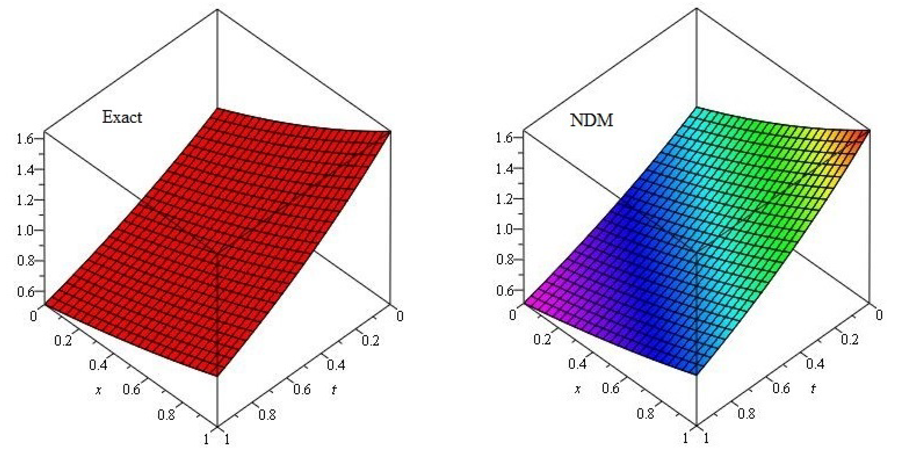
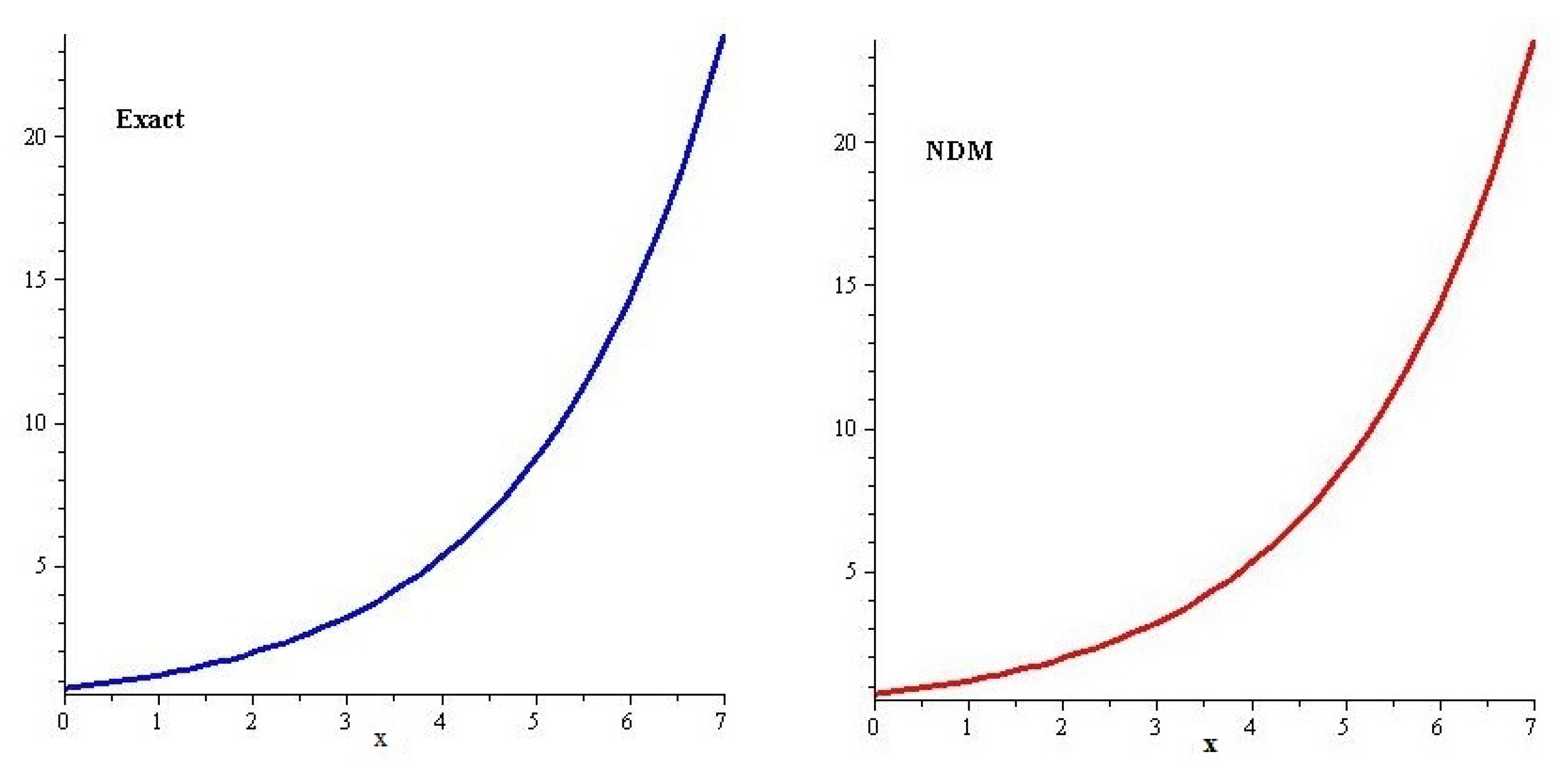
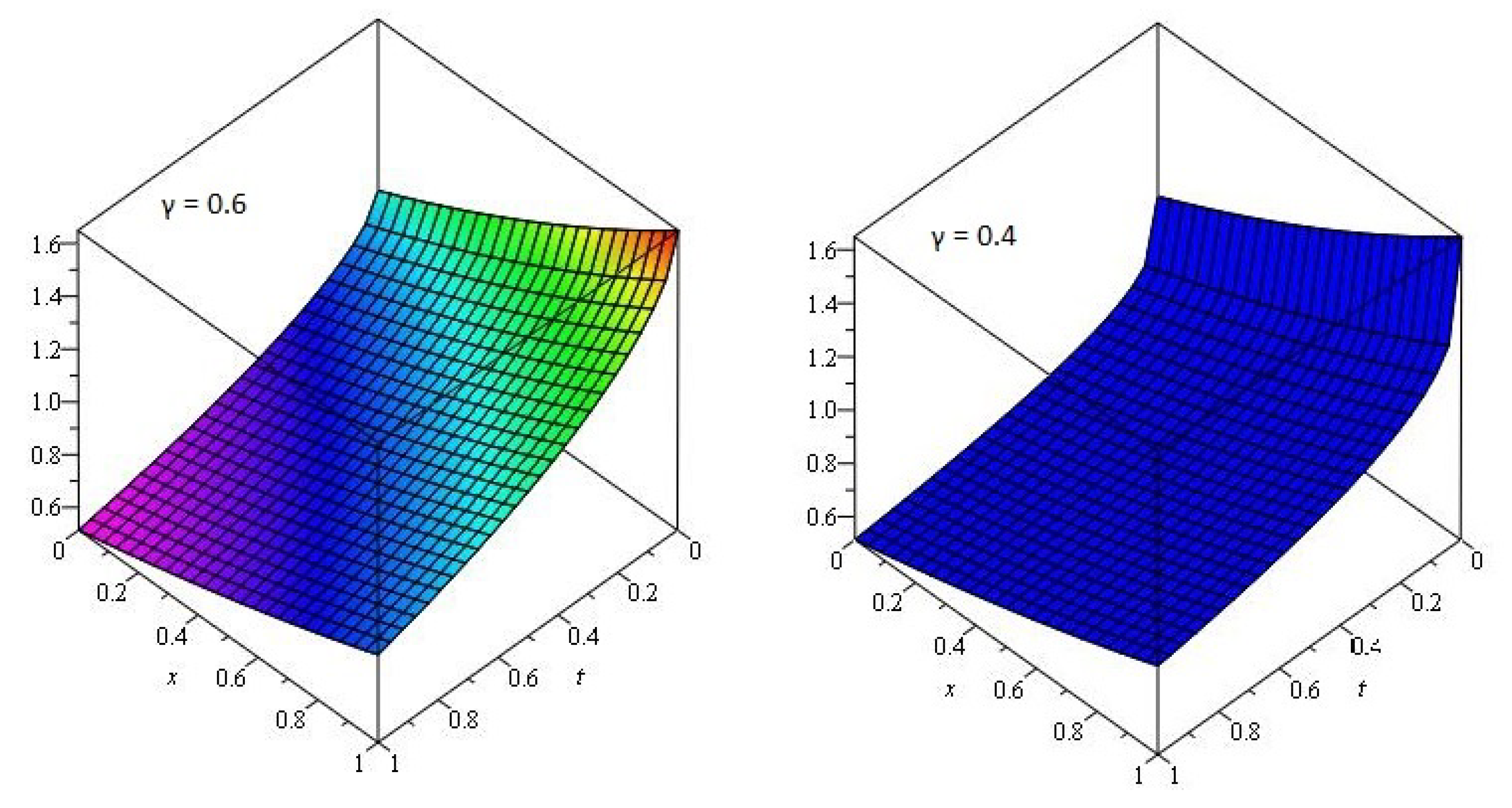
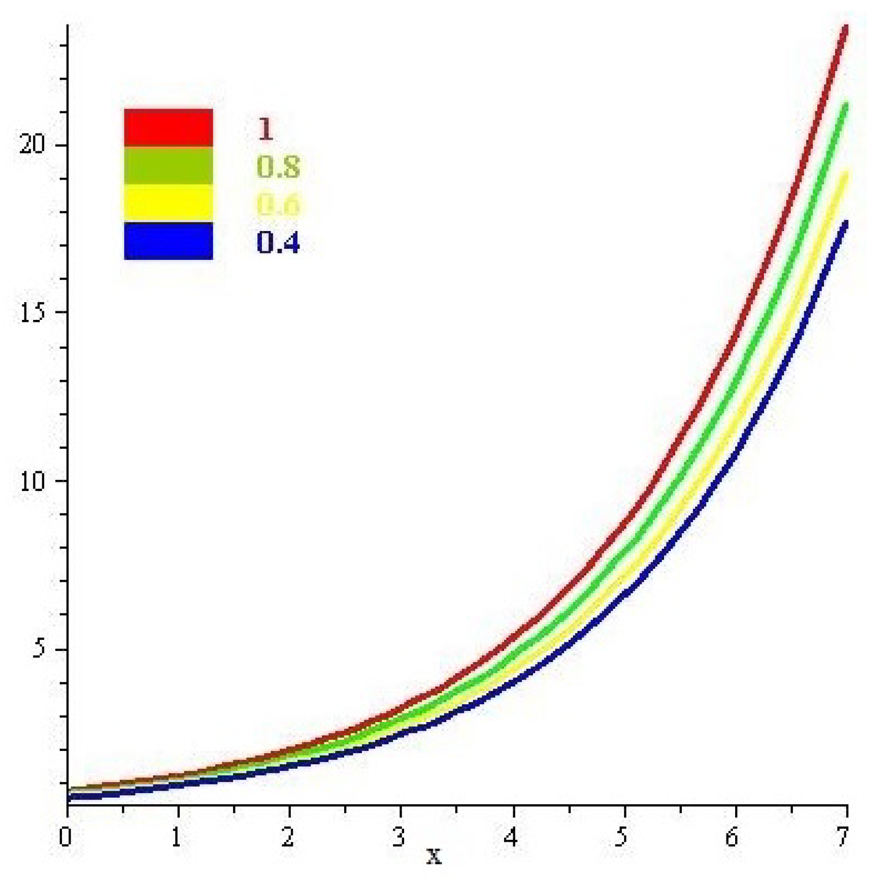
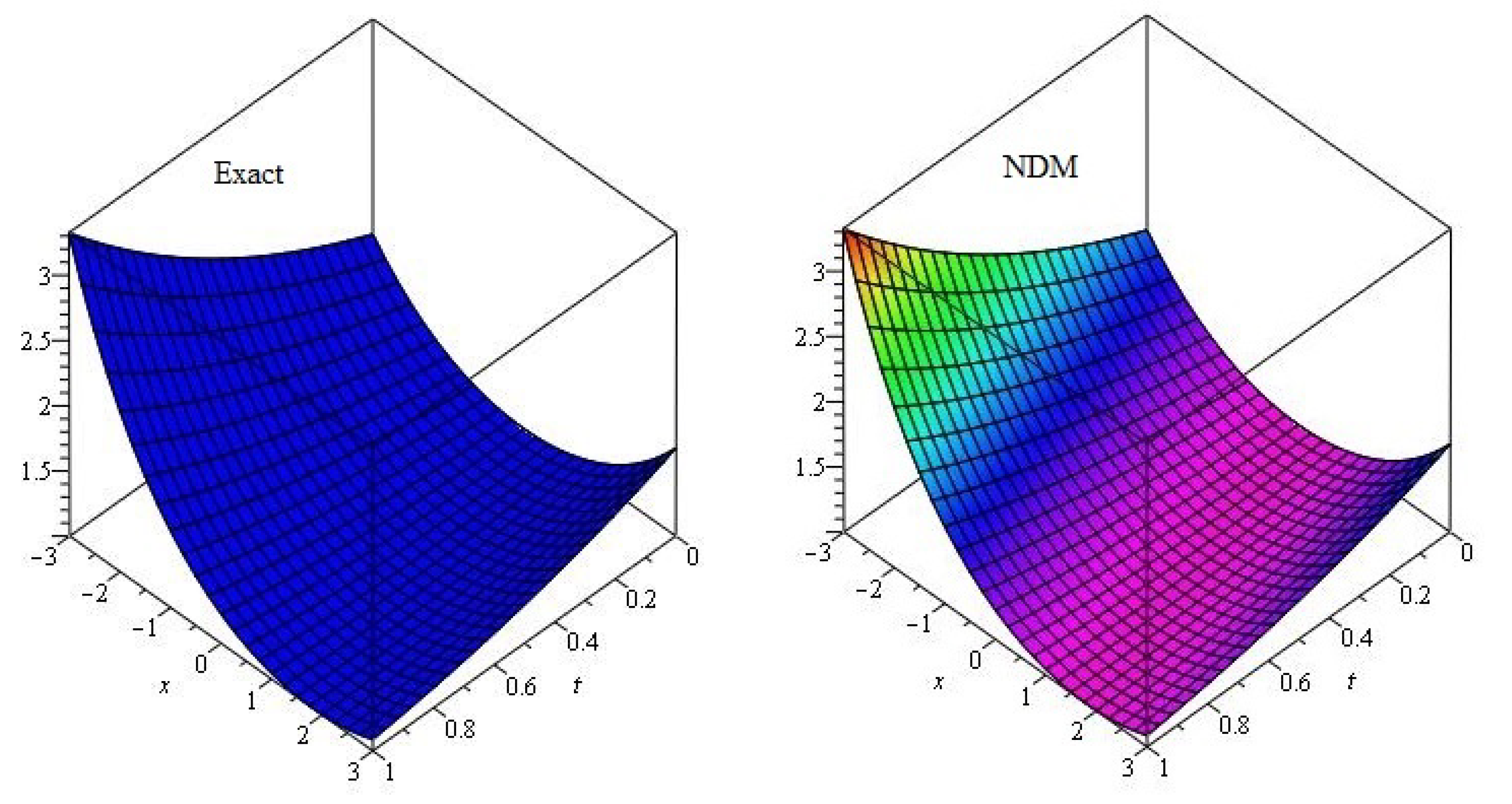
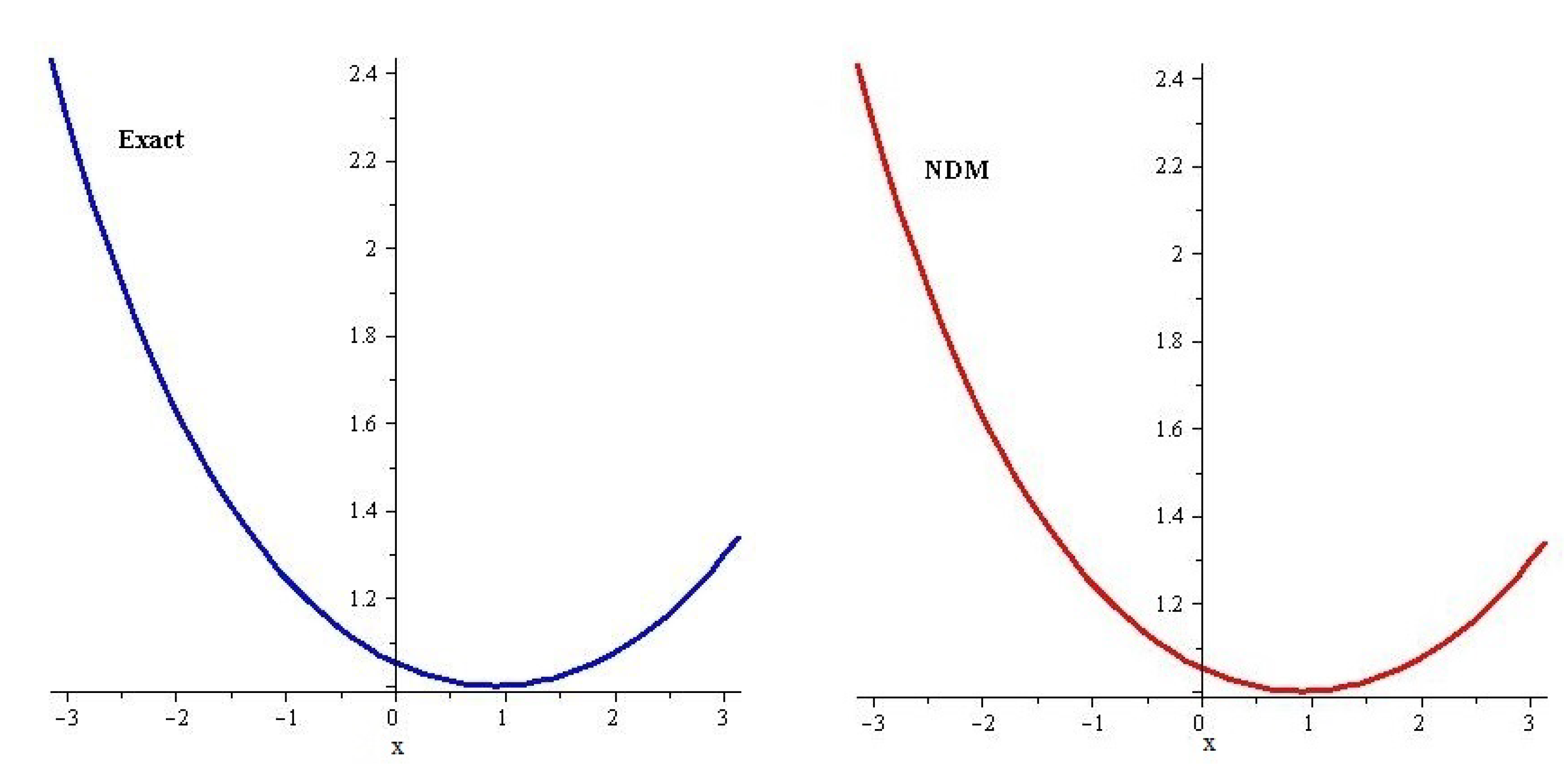
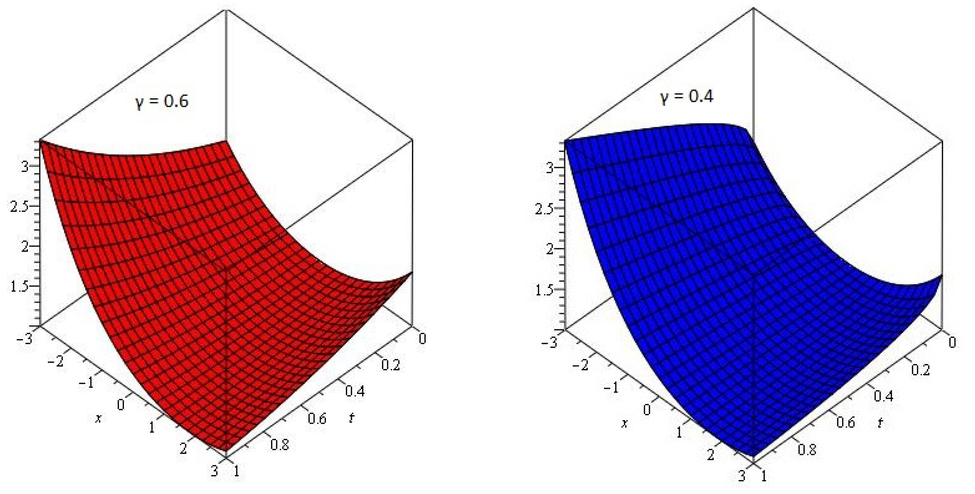
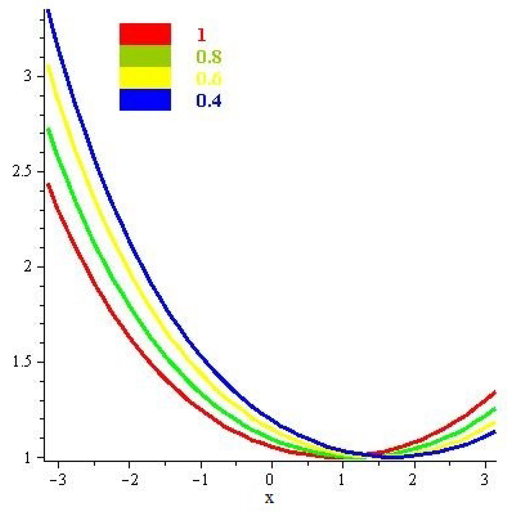
In Figure 1 and Figure 2, the NDM and actual solution of Example 1 are plotted. It is observed that NDM solutions are in closed contact with the exact solutions of Example 1. In Figure 3 and Figure 4, the solutions of Example 1 at various fractional-order of the derivatives are plotted. The graphical representation has shown the convergence phenomena of fractional-order solution towards the solution at integer order of Example 1.

Example 2.

Consider the following nonlinear time-fractional Fornberg–Whitham equation [18]

$$D_t^{\gamma }\mu -D_{xxt}\mu +D_x\mu =\mu D_{xxx}\mu -\mu D_x\mu +3D_x\mu D_{xx}\mu ,t>0,0<\gamma \le 1,$$

(25)

with initial condition

$$\mu (x,0)={cosh}^2\left(\frac{x}{4}\right),$$

(26)

Applying natural transformation of Equation (25),

$$\frac{s^{\gamma }}{{\omega }^{\gamma }}{N}^{+}\left[\mu (x,t)\right]-\frac{s^{\gamma -1}}{{\omega }^{\gamma }}\mu (x,0)=N^{+}\left[D_{xxt}\mu -D_x\mu +\mu D_{xxx}\mu -\mu D_x\mu +3D_x\mu D_{xx}\mu \right].$$

$$N^{+}\left[\mu (x,t)\right]-\frac{1}{s}\mu (x,0)=\frac{{\omega }^{\gamma }}{s^{\gamma }}{N}^{+}\left[D_{xxt}\mu -D_x\mu +\mu D_{xxx}\mu -\mu D_x\mu +3D_x\mu D_{xx}\mu \right].$$

Using inverse natural transformation

$$\mu (x,t)=N^{-}\left[\frac{\mu (x,0)}{s}-\frac{{\omega }^{\gamma }}{s^{\gamma }}{N}^{+}\left[D_{xxt}\mu -D_x\mu +\mu D_{xxx}\mu -\mu D_x\mu +3D_x\mu D_{xx}\mu \right]\right].$$

Applying the ADM process, we have

$${\mu }_0(x,t)=N^{-}\left[\frac{\mu (x,0)}{s}\right]=N^{-}\left[\frac{{cosh}^2\left(\frac{x}{4}\right)}{s}\right],$$

$${\mu }_0(x,t)={cosh}^2\left(\frac{x}{4}\right),$$

(27)

$$\sum _{\ell =0}^{\infty }{\mu }_{\ell +1}(x,t)=N^{-}\left[\frac{{\omega }^{\gamma }}{s^{\gamma }}{N}^{+}\left[\sum _{\ell =0}^{\infty }{(D_{xxt}\mu )}_{\ell }-\sum _{\ell =0}^{\infty }{(D_x\mu )}_{\ell }+\sum _{\ell =0}^{\infty }{A}_{\ell }-\sum _{\ell =0}^{\infty }{B}_{\ell }+3\sum _{\ell =0}^{\infty }{C}_{\ell }\right]\right],\ell =0,1,2,\cdots$$

$$\begin{array}{cc}\hfill A_0(\mu D_{xxx}\mu )& ={\mu }_0{D}_{xxx}{\mu }_0,\hfill \\ \hfill A_1(\mu D_{xxx}\mu )& ={\mu }_0{D}_{xxx}{\mu }_1+{\mu }_1{D}_{xxx}{\mu }_0,\hfill \\ \hfill A_2(\mu D_{xxx}\mu )& ={\mu }_1{D}_{xxx}{\mu }_2+{\mu }_1{D}_{xxx}{\mu }_1+{\mu }_2{D}_{xxx}{\mu }_0,\hfill \end{array}$$

$$\begin{array}{c}{B}_0(\mu D_x\mu )={\mu }_0{D}_x{\mu }_0,\hfill \\ B_1(\mu D_x\mu )={\mu }_0{D}_x{\mu }_1+{\mu }_1{D}_x{\mu }_0,\hfill \\ B_2(\mu D_x\mu )={\mu }_1{D}_x{\mu }_2+{\mu }_1{D}_x{\mu }_1+{\mu }_2{D}_x{\mu }_0.\hfill \end{array}$$

$$\begin{array}{cc}\hfill C_0(D_x\mu D_{xx}\mu )& =D_x{\mu }_0{D}_{xx}{\mu }_0,\hfill \\ \hfill C_1(D_x\mu D_{xx}\mu )& =D_x{\mu }_0{D}_{xx}{\mu }_1+D_x{\mu }_1{D}_{xx}{\mu }_0,\hfill \\ \hfill C_2(D_x\mu D_{xx}\mu )& =D_x{\mu }_1{D}_{xx}{\mu }_2+D_x{\mu }_1{D}_{xx}{\mu }_1+D_x{\mu }_2{D}_{xx}{\mu }_0,\hfill \end{array}$$

for $\ell =1$

$$\begin{array}{cc}\hfill & {\mu }_1(x,t)=N^{-}\left[\frac{{\omega }^{\gamma }}{s^{\gamma }}{N}^{+}\left[{(D_{xxt}\mu )}_0-{(D_x\mu )}_0+A_0-B_0+3C_0\right]\right],\hfill \\ \hfill & {\mu }_1(x,t)=-\frac{11}{32}{N}^{-}\left[\frac{{\omega }^{\gamma }sinh\left(\frac{x}{2}\right)}{s^{\gamma +1}}\right]=-0.3437sinh\left(\frac{x}{4}\right)\frac{t^{\gamma }}{\mathsf{\Gamma }(\gamma +1)},\hfill \end{array}$$

(28)

for $\ell =2$

$$\begin{array}{cc}\hfill & {\mu }_2(x,t)=N^{-}\left[\frac{{\omega }^{\gamma }}{s^{\gamma }}{N}^{+}\left[{(D_{xxt}\mu )}_1-{(D_x\mu )}_1+A_1-B_1+3C_1\right]\right],\hfill \\ \hfill & {\mu }_2(x,t)=-0.08593sinh\left(\frac{x}{4}\right)\frac{t^{\gamma }}{\mathsf{\Gamma }(\gamma +1)}+0.11816cosh\left(\frac{x}{4}\right)\frac{t^{2\gamma }}{\mathsf{\Gamma }(2\gamma +1)},\hfill \end{array}$$

(29)

for $\ell =3$

$$\begin{array}{cc}\hfill & {\mu }_3(x,t)=N^{-}\left[\frac{{\omega }^{\gamma }}{s^{\gamma }}{N}^{+}\left[{(D_{xxt}\mu )}_2-{(D_x\mu )}_2+A_2-B_2+3C_2\right]\right],\hfill \\ \hfill & {\mu }_3(x,t)=-0.08593sinh\left(\frac{x}{4}\right)\frac{t^{\gamma }}{\mathsf{\Gamma }(\gamma +1)}+0.11816cosh\left(\frac{x}{4}\right)\frac{t^{2\gamma }}{\mathsf{\Gamma }(2\gamma +1)}-0.02707sinh\left(\frac{x}{4}\right)\frac{t^{3\gamma }}{\mathsf{\Gamma }(3\gamma +1)}.\hfill \end{array}$$

(30)

The NDM result for problem 2 is

$$\mu (x,t)={\mu }_0(x,t)+{\mu }_1(x,t)+{\mu }_2(x,t)+{\mu }_3(x,t)+{\mu }_4(x,t)\cdots .$$

$$\begin{array}{cc}\hfill \mu (x,t)=& {cosh}^2\left(\frac{x}{4}\right)-0.3437sinh\left(\frac{x}{4}\right)\frac{t^{\gamma }}{\mathsf{\Gamma }(\gamma +1)}-0.08593sinh\left(\frac{x}{4}\right)\frac{t^{\gamma }}{\mathsf{\Gamma }(\gamma +1)}\hfill \\ \hfill & +0.11816cosh\left(\frac{x}{4}\right)\frac{t^{2\gamma }}{\mathsf{\Gamma }(2\gamma +1)}-0.08593sinh\left(\frac{x}{4}\right)\frac{t^{\gamma }}{\mathsf{\Gamma }(\gamma +1)}\hfill \\ \hfill & +0.11816cosh\left(\frac{x}{4}\right)\frac{t^{2\gamma }}{\mathsf{\Gamma }(2\gamma +1)}-0.02707sinh\left(\frac{x}{4}\right)\frac{t^{3\gamma }}{\mathsf{\Gamma }(3\gamma +1)}-\cdots .\hfill \end{array}$$

The exact result is;

$$\mu (x,t)={cosh}^2\left(\frac{x}{4}-\frac{11t}{24}\right).$$

In Figure 5 and Figure 6, the solution graph of exact and NDM of Example 2 at integer-order are plotted. The closed relation is observed between NDM and exact solution of Example 2. In Figure 7 and Figure 8, the fractional-order solutions of Example 2 are presented. The graphical representation have confirmed the different dynamics of Example 2, which are correlated with each other.

5. Conclusions

In the current work. an innovative technique is used to find the solution of fractional Fornberg-Whitham equations. The fractional-derivatives are discussed within Caputo operator. The solutions are determined for fractional-order problems and an aesthetically a strong relation is found. The fractional models have shown convergence to the ordinary model as the order of the derivative tends towards to an integer. The graphical representation has provided similar behavior of actual and derived results. It is also noted the current method needs small calculation and higher convergence to achieve the solution of the targeted problems.

References

- Acan, O.; Firat, O.; Keskin, Y. Conformable variational iteration method, conformable fractional reduced differential transform method and conformable homotopy analysis method for non-linear fractional partial differential equations. Waves Random Complex Media 2020, 30, 250–268. [Google Scholar] [CrossRef]
- Najafi, R. Group-invariant solutions for time-fractional Fornberg-Whitham equation by Lie symmetry analysis. Comput. Methods Differ. Equ. 2020, 8, 251–258. [Google Scholar]
- Hörmann, G.; Okamoto, H. Weak periodic solutions and numerical case studies of the Fornberg-Whitham equation. arXiv 2018, arXiv:1807.02320. [Google Scholar] [CrossRef] [Green Version]
- Zhou, J.; Tian, L. A type of bounded traveling wave solutions for the Fornberg–Whitham equation. J. Math. Anal. Appl. 2008, 346, 255–261. [Google Scholar] [CrossRef] [Green Version]
- Moldabayev, D.; Kalisch, H.; Dutykh, D. The Whitham equation as a model for surface water waves. Phys. D Nonlinear Phenom. 2015, 309, 99–107. [Google Scholar] [CrossRef]
- Lenells, J. Traveling wave solutions of the Camassa–Holm and Korteweg–de Vries Equations. J. Nonlinear Math. Phys. 2004, 11, 508–520. [Google Scholar] [CrossRef]
- Camassa, R.; Holm, D. An integrable shallow wave equation with peaked solitons. Phys. Rev. Lett. 1993, 71, 1661–1664. [Google Scholar] [CrossRef] [Green Version]
- Lenells, J. Traveling wave solutions of the Camassa–Holm equation. J. Differ. Equ. 2005, 217, 393–430. [Google Scholar] [CrossRef] [Green Version]
- Liu, Z.; Chen, C. Compactons in a general compressible hyperelastic rod. Chaos Soliton Fractals 2004, 22, 627–640. [Google Scholar] [CrossRef]
- Parkes, E.J.; Vakhnenko, V.O. Explicit solutions of the Camassa–Holm equation. Chaos Solitons Fractals 2005, 26, 1309–1316. [Google Scholar] [CrossRef]
- Whitham, G.B. Variational methods and applications to water waves. Philos. Trans. R. Soc. Lond. Ser. A Math. Phys. Sci. 1967, 299, 6–25. [Google Scholar]
- Fornberg, B.; Whitham, G.B. A numerical and theoretical study of certain nonlinear wave phenomena. Philos. Trans. R. Soc. Lond. Ser. A Math. Phys. Sci. 1978, 289, 373–404. [Google Scholar]
- Purohit, S.D. Solutions of fractional partial differential equations of quantum mechanics. Adv. Appl. Math. Mech. 2013, 5, 639–651. [Google Scholar] [CrossRef]
- Singh, J.; Kumar, D.; Kumar, S. New treatment of fractional Fornberg–Whitham equation via Laplace transform. Ain Shams Eng. J. 2013, 4, 557–562. [Google Scholar] [CrossRef] [Green Version]
- Iyiola, O.S.; Ojo, G.O. On the analytical solution of Fornberg–Whitham equation with the new fractional derivative. Pramana 2015, 85, 567–575. [Google Scholar] [CrossRef]
- Kumar, D.; Singh, J.; Baleanu, D. A new analysis of the Fornberg-Whitham equation pertaining to a fractional derivative with Mittag-Leffler-type kernel. Eur. Phys. J. Plus 2018, 133, 70. [Google Scholar] [CrossRef]
- Gupta, P.K.; Singh, M. Homotopy perturbation method for fractional Fornberg–Whitham equation. Comput. Math. Appl. 2011, 61, 250–254. [Google Scholar] [CrossRef]
- Abidi, F.; Omrani, K. Numerical solutions for the nonlinear Fornberg-Whitham equation by He’s method. Int. J. Mod. Phys. B 2011, 25, 4721–4732. [Google Scholar] [CrossRef]
- Li, Q.; Sun, S.; Han, Z.; Zhao, Y. On the existence and uniqueness of solutions for initial value problem of nonlinear fractional differential equations. In Proceedings of the 2010 IEEE/ASME International Conference on Mechatronic and Embedded Systems and Applications, Qingdao, China, 15–17 July 2010; pp. 452–457. [Google Scholar]
- Bacani, D.B.; Tahara, H. Existence and uniqueness theorem for a class of singular nonlinear partial differential equations. Publ. Res. Inst. Math. Sci. 2012, 48, 899–917. [Google Scholar] [CrossRef] [Green Version]
- Dannan, F.M.; Saleeby, E.G. An existence and uniqueness theorem for n-th order functional differential equations. Int. J. Pure Appl. Math. 2013, 84, 193–200. [Google Scholar] [CrossRef] [Green Version]
- Gao, X.; Lai, S.; Chen, H. The stability of solutions for the Fornberg–Whitham equation in L1(R) space. Bound. Value Probl. 2018, 2018, 142. [Google Scholar] [CrossRef]
- Shen, C.; Gao, A. Optimal distributed control of the Fornberg–Whitham equation. Nonlinear Anal. Real World Appl. 2015, 21, 127–141. [Google Scholar] [CrossRef]
- Jajarmi, A.; Yusuf, A.; Baleanu, D.; Inc, M. A new fractional HRSV model and its optimal control: A non-singular operator approach. Phys. A Stat. Mech. Its Appl. 2019, 547, 123860. [Google Scholar] [CrossRef]
- Tuan, N.H.; Baleanu, D.; Thach, T.N.; O’Regan, D.; Can, N.H. Approximate solution for a 2-D fractional differential equation with discrete random noise. Chaos Solitons Fractals 2020, 133, 109650. [Google Scholar] [CrossRef]
- Anh Triet, N.; Van Au, V.; Dinh Long, L.; Baleanu, D.; Huy Tuan, N. Regularization of a terminal value problem for time fractional diffusion equation. Math. Methods Appl. Sci. 2020, 43, 3850–3878. [Google Scholar] [CrossRef]
- Tuan, N.H.; Baleanu, D.; Thach, T.N.; O’Regan, D.; Can, N.H. Final value problem for nonlinear time fractional reaction–diffusion equation with discrete data. J. Comput. Appl. Math. 2020, 376, 112883. [Google Scholar] [CrossRef]
- Şenol, M.; Iyiola, O.S.; Kasmaei, H.D.; Akinyemi, L. Efficient analytical techniques for solving time-fractional nonlinear coupled Jaulent–Miodek system with energy-dependent Schrödinger potential. Adv. Differ. Equ. 2019, 2019, 462. [Google Scholar] [CrossRef]
- Akinyemi, L.; Iyiola, O. Exact and approximate solutions of time-fractional models arising from physics via Shehu transform. Math. Methods Appl. Sci. 2020. [Google Scholar] [CrossRef]
- Akinyemi, L.; Iyiola, O.S. A reliable technique to study nonlinear time-fractional coupled Korteweg–de Vries equations. Adv. Differ. Equ. 2020, 2020, 1–27. [Google Scholar] [CrossRef] [Green Version]
- Shah, R.; Khan, H.; Baleanu, D.; Kumam, P.; Arif, M. The analytical investigation of time-fractional multi-dimensional Navier–Stokes equation. Alex. Eng. J. 2020, in press. [Google Scholar] [CrossRef]
- Jan, R.; Xiao, Y. Effect of partial immunity on transmission dynamics of dengue disease with optimal control. Math. Methods Appl. Sci. 2019, 42, 1967–1983. [Google Scholar] [CrossRef]
- Jan, R.; Xiao, Y. Effect of pulse vaccination on dynamics of dengue with periodic transmission functions. Adv. Differ. Equ. 2019, 1, 368. [Google Scholar] [CrossRef] [Green Version]
- Mahmood, S.; Shah, R.; Arif, M. Laplace Adomian Decomposition Method for Multi Dimensional Time Fractional Model of Navier-Stokes Equation. Symmetry 2019, 11, 149. [Google Scholar] [CrossRef] [Green Version]
- Shah, R.; Khan, H.; Farooq, U.; Baleanu, D.; Kumam, P.; Arif, M. A New Analytical Technique to Solve System of Fractional-Order Partial Differential Equations. IEEE Access 2019, 7, 150037–150050. [Google Scholar] [CrossRef]
- Shah, R.; Khan, H.; Kumam, P.; Arif, M. An analytical technique to solve the system of nonlinear fractional partial differential equations. Mathematics 2019, 7, 505. [Google Scholar] [CrossRef] [Green Version]
- Shah, R.; Khan, H.; Baleanu, D.; Kumam, P.; Arif, M. A novel method for the analytical solution of fractional Zakharov–Kuznetsov equations. Adv. Differ. Equ. 2019, 2019, 1–14. [Google Scholar] [CrossRef]
- Khan, H.; Farooq, U.; Shah, R.; Baleanu, D.; Kumam, P.; Arif, M. Analytical Solutions of (2+ Time Fractional Order) Dimensional Physical Models, Using Modified Decomposition Method. Appl. Sci. 2020, 10, 122. [Google Scholar] [CrossRef] [Green Version]
- Shah, R.; Farooq, U.; Khan, H.; Baleanu, D.; Kumam, P.; Arif, M. Fractional view analysis of third order Kortewege-De Vries equations, using a new analytical technique. Front. Phys. 2020, 7, 244. [Google Scholar] [CrossRef] [Green Version]
- Khan, Z.H.; Khan, W.A. N-transform-properties and applications. NUST J. Eng. Sci. 2008, 1, 127–133. [Google Scholar]
- Rawashdeh, M.S.; Maitama, S. Solving nonlinear ordinary differential equations using the NDM. J. Appl. Anal. Comput. 2015, 5, 77–88. [Google Scholar]
- Rawashdeh, M.S.; Maitama, S. Solving PDEs using the natural decomposition method. Nonlinear Stud. 2016, 23, 63–72. [Google Scholar]
- Khan, H.; Shah, R.; Kumam, P.; Arif, M. Analytical Solutions of Fractional-Order Heat and Wave Equations by the Natural Transform Decomposition Method. Entropy 2019, 21, 597. [Google Scholar] [CrossRef] [Green Version]
- Rawashdeh, M.S.; Maitama, S. Solving coupled system of nonlinear PDE’s using the natural decomposition method. Int. J. Pure Appl. Math. 2014, 92, 757–776. [Google Scholar] [CrossRef] [Green Version]
- Khan, H.; Shah, R.; Baleanu, D.; Kumam, P.; Arif, M. Analytical Solution of Fractional-Order Hyperbolic Telegraph Equation, Using Natural Transform Decomposition Method. Electronics 2019, 8, 1015. [Google Scholar] [CrossRef] [Green Version]
- Rawashdeh, M.S. The fractional natural decomposition method: Theories and applications. Math. Methods Appl. Sci. 2017, 40, 2362–2376. [Google Scholar] [CrossRef]
- Shah, R.; Khan, H.; Mustafa, S.; Kumam, P.; Arif, M. Analytical Solutions of Fractional-Order Diffusion Equations by Natural Transform Decomposition Method. Entropy 2019, 21, 557. [Google Scholar] [CrossRef] [Green Version]
- Miller, K.S.; Ross, B. An Introduction to the Fractional Calculus and Fractional Differential Equations; Wiley: New York, NY, USA, 1993. [Google Scholar]
- Hilfer, R. Applications of Fractional Calculus in Physics; World Sci. Publishing: River Edge, NJ, USA, 2000. [Google Scholar]
- Agarwal, R.; Lakshmikantham, V.; Nieto, J. On the concept of solution for fractional differential equations with uncertainty. Nonlinear Anal. Theory Methods Appl. 2010, 72, 2859–2862. [Google Scholar] [CrossRef]
- Belgacem, F.B.M.; Silambarasan, R. Maxwell’s equations solutions by means of the natural transform. Int. J. Math. Eng. Sci. Aerosp. 2012, 3, 313–323. [Google Scholar]
Figure 1.
Exact and NDM solutions at of Example 1.
Figure 2.
Figure 3.
The NDM solutions of different valve of of Example 1.
Figure 4.
Solution graph of Example 1, at various value of .
Figure 5.
The graph of exact and approximate solution of Example 2.
Figure 6.
Figure 7.
The NDM solutions of different valve of γ of Example 2.
Figure 8.
The graph of Example 2, for different value of γ.