Designing Limit-Cycle Suppressor Using Dithering and Dual-Input Describing Function Methods

Abstract

This paper described a method to design a limit-cycle suppressor. The dithering technique was used to eliminate self-sustained oscillations or limit cycles. Otherwise, the Dual Input Describing Function (DIDF) method was applied to design dither parameters and analyze the existence of limit cycles. This method was done in a nonlinear system with relay nonlinearity using three standard dither signals, namely sine, triangle, and square waves. The aim of choosing varying dithers was to investigate the effect of dither shapes and the minimum amplitude required for the quenching strategy. First, the possibility and amplitude of limit cycles were determined graphically on the DIDF curve. Then, the minimum amplitude of dither was calculated based on the DIDF analysis. Finally, a simulation was built to verify the analytical work using a digital computer. The simulation results were related to the analysis results. It was evident that the dithering technique is a simple way to suppress limit cycles in a nonlinear system. This paper also presented that dither is an amplitude function, and square-wave dither has the minimum amplitude to quench limit cycles.

1. Introduction

Self-sustained oscillation or limit cycles is an important phenomenon that is encountered in a nonlinear system. Some researchers have been devoted to study the limit cycle, i.e., Huang and Yap [1] introduced an algorithmic approach to analyze the limit cycle bifurcation. This method is implemented in Maple and is done effectively. By using the multiple switching curve, Yang [2] analyzed the bifurcation of limit cycles for a piecewise near-Hamilton system. This showed that the number of limit cycles is affected by the number of switching curves. Balajewicz and Dowel [3] presented that the Volterra reduced-order model is capable of modeling aerodynamically induced limit-cycle oscillations efficiently and accurately. This analysis method was demonstrated using a NACA 0012 benchmark model.

Limit-cycle can arise from nonlinearities that are inherent in nonlinear systems. On the other hand, this oscillation cannot be derived from a linear method. Therefore, a nonlinear system analysis technique must be developed [4]. As this phenomenon can affect the system’s overall behavior, an approach to predict its existence and stability analysis is necessary. The methods based on analytical analysis have been widely discussed throughout the literature. Hayes and Marques [5], followed by Shukla and Patil [6], predicted the limit cycle amplitude and frequency by the harmonic balance method. In [5], a formulation of High Dimensional Harmonic Balance is employed to determine the condition of the limit cycle. This formulation is exploited in limit cycle conditions without evoking the cost of the time-accurate simulation. Shukla and Patil reported the harmonic balance as a method to estimate the limit cycle frequency and amplitude displayed by a flutter mode. Zhang and Wu [7] proved that the homotopy analysis is a highly accurate method to approximate the limit cycles of a coupled oscillator. The authors in [8] presented the Holding type I and II to examine the variable carrying capacity effect on the predator–prey dynamic system and it is analyzed using the numerical solution and stability analysis under a Hopf bifurcation theorem. Denimal et al. [9] proposed the modal amplitude stability analysis called the Generalized Modal Amplitude Stability Analysis to estimate the limit cycle. This method is also used to identify the contributions and evolutions of unstable modes. The powerful mathematical approach to analyze and improve the nonlinear behavior is known as the Describing Function method (DF) [10]. The main idea of the DF method is to replace the nonlinear element with its equivalent linear. This method is mainly used to predict the limit cycles of nonlinear systems [4]. Several new results for predicting the limit cycles using the DF approach have been recently announced. DF has been applied to predict and investigate the limit cycle in Stirling Engine [11] and pressurized gas turbine combustor [12]. DF has also been used as a method to analyze the nonlinear system [13], such as analysis stability of Chaotic PWM Boost Converters [14], or stability analysis of dynamic nonlinear interval type-2 TSK fuzzy control [15].

In order to enhance the system’s performance, the limit cycle existence should be eliminated. Recently, several works have been carried out aimed at eliminating the limit cycle. A nonlinear state feedback control is proposed in [16], controlling the limit cycle oscillation in an aero-elastic system. The harmonic balance method and the numerical continuation technique were used to produce an analytical estimate of the initial velocity of the limit cycle. Girija et al. [17] showed that the reduced state Kalman filter scheme eliminates the limit cycle in DC-DC converter completely and is more efficient computationally. Kumar et al. [18] developed a new mechanism for stabilizing the undesirable limit cycle in a chaotic attractor. This method is demonstrated with a bi-stable Duffing oscillator. In [19], the authors implemented a linear controller based on a frequency response to eliminate the limit cycle in the inverted pendulum on a cart. This control strategy has been successfully applied and is verified by experimental means.

The other interesting method which can be adapted to compensate for the nonlinearities’ effects in a feedback control system, including limit cycles, is the dithering technique. The method was done by injecting an extra input signal called dither signal just ahead of the nonlinearity, causing the nonlinear system to narrow so it could be stabilized. The use of dither signal to turn limit cycles off is referred to as signal signals’ stabilization [20]. The dithering technique has been widely used in different fields such as electronics [21,22], mechanics [23,24], and control system [25,26]. The modified direct torque control with dithering to increase the performance of the induction motor drive is proposed by Behera and Das [27,28]. It was investigated that the dither signal injection increases the inverter switching frequency. The same strategy was also conducted by Kadjoudj et al. [29], which has been applied to the PMSM drive. The dither injection technique has also been used for quenching the chaotic system. From Chang, it is inferred that by adding the dither signal into the system, the chaos occurs in a magnetically levitated system [30] and in electromechanical valve actuators [31] was successfully eliminated. In reference [32], the dither technique has been examined for controlling chaos in an automotive suspension system. Here, the chaotic behavior is converted into periodic motion. However, all these reported works lack an analytical approach in designing the dither signal including the amplitude, frequency, and shape of the dither signal. Even so, these parameters are important to note [33]. Meanwhile, the shape of the dither signal could affect the transient response system [34,35].

In this present study, we use the dithering technique to suppress the limit cycle in a relay nonlinear servo system and study the performance of three kinds of dither shapes, namely sinusoidal, triangle, and square wave. In order to design the dither amplitude, the modified DF method named Duat Input Describing Function (DIDF) was applied. DIDF was examined by West et al. [36] to solve the possible limit cycles in a nonlinear system. Here the DIDF is defined as the ratio of the amplitude of the desired frequency components (required for the analysis) in the output waveform to the amplitude of the components of the same frequency in the input waveform. It was shown that the DIDF could be used to evaluate the limit-cycle stability. Currently, the DIDF approach is also carried out in research. In Reference [37], the unknown parameters for second-order-plus-dead-time and first-order-plus-dead-time are obtained using DIDF. In this method, the setting of relay bias does not need to be changed during load disturbance to obtain the process information. Choe [38,39] introduced a method to enhance the PID controller performance by using the DIDF characteristic. Another term of DIDF is called pseudo-DF.

The main contributions of this study are briefly given in the following statement: (1) The dithering techniques to suppress the limit cycles on a relay feedback loop are proposed; (2) The step of designing dither signal analytically through the DIDF method is presented; (3) A simple simulation build in Matlab-Simulink software is taken as an example to show the effectiveness of the purposed method and to verify the analytical method; (4) The results of the analysis and simulation also pointed out the minimum dither amplitude required from three common dither shapes and the effect of dither signal shape.

The paper is organized as follows. The method to design dither signal amplitude based on the DIDF approach is described in Section 2. Section 3 illustrated the Matlab/Simulink simulation to verify the designing method and the effectiveness of the dithering technique in the relay feedback system. The conclusions and future works are given in Section 4.

2. Method

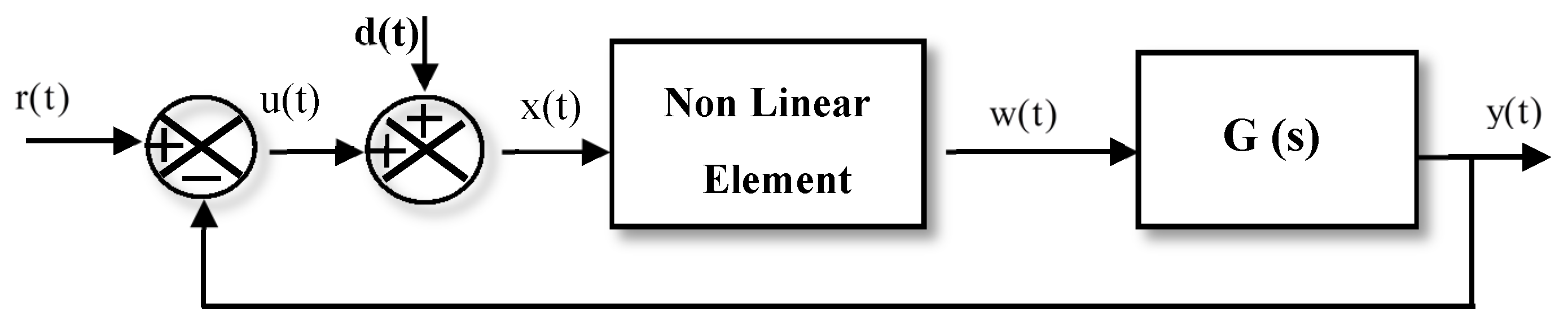
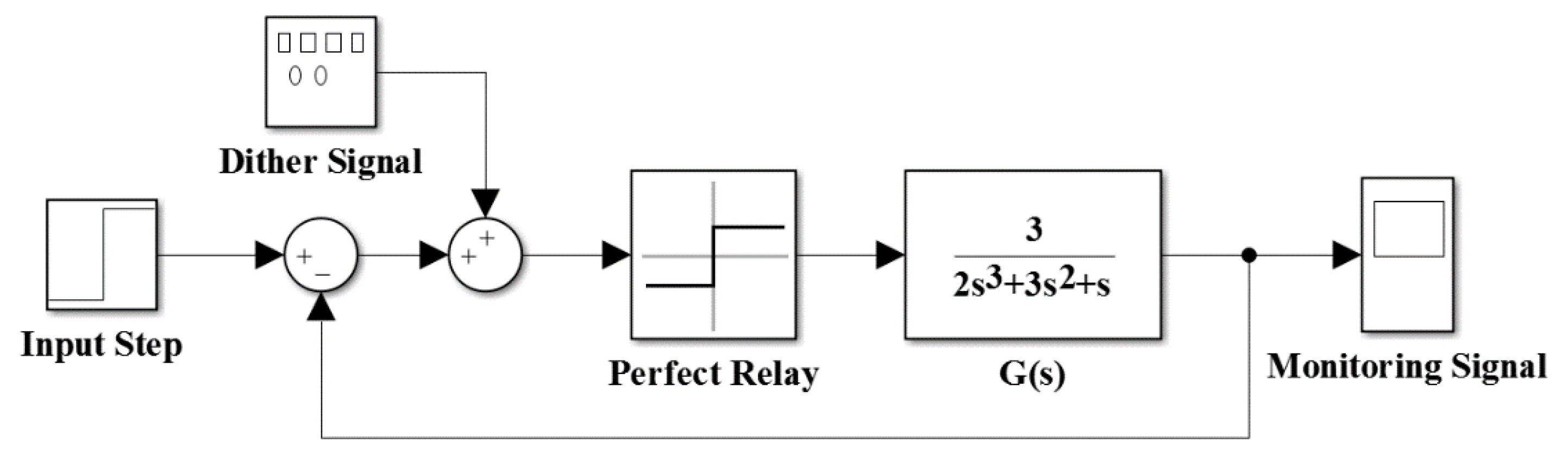
Initially, the DF method was used to analyze the feedback control system containing a nonlinear element. It was basically developed only for sinusoidal inputs. The development was done to analyze the system with the addition of a stabilizing signal, named the DIDF method. This method is based on the consideration of two sinusoids applied at the input of the nonlinear element. In that case, a high suitable frequency signal (dither) is injected externally to modify the characteristics of the nonlinearity, which often has a linearizing effect on the nonlinear element and stabilizes the system. The concept of DIDF was first introduced by West et al. [36], and then extended by Gibson and Sridhar [33]. For the system in which dithers are present, as shown in Figure 1, the investigation of signal stabilization named dither via DF theory can be executed by the use of the DIDF approach.

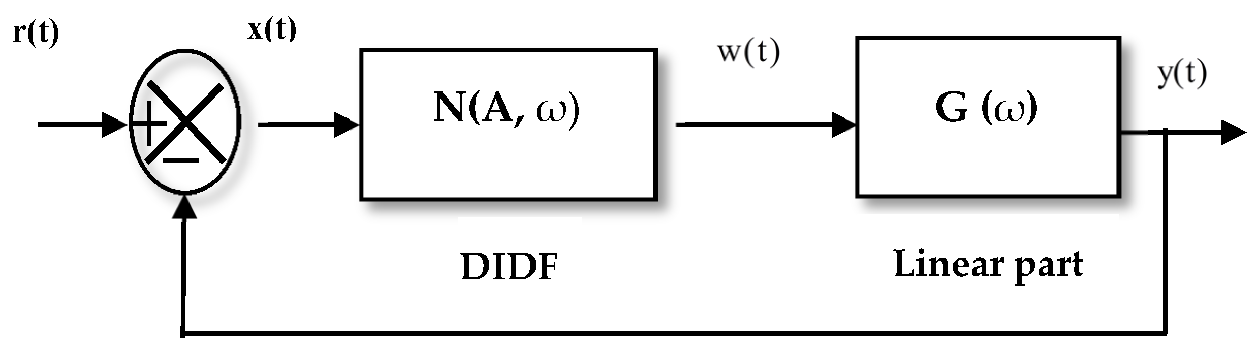
For implementing the DIDF method, it is important to represent the nonlinear system as the block diagram exhibit in Figure 2. As shown in this figure, the system contains negative feedback associated with nonlinear and linear terms. In this method, dithers and the nonlinear element are replaced with an equivalent nonlinear element or DIDF.

The possibility of the limit cycle existence, including the suppression, could be investigated in the servo system with dither injection, as shown in Figure 1.

In this system, the linear part is represented by the transfer function, which contains an ideal relay as a nonlinear element, described as

$$\mathrm{G}(\mathrm{s})=\frac{3}{\mathrm{s}(\mathrm{s}+1)(2\mathrm{s}+1)}$$

(1)

The DIDF analysis is used to predict the limit-cycle amplitude. The basic approach to achieve that is applying Nyquist criterion in linear control to the equivalent system. According to the Nyquist criterion, limit cycles or self-sustained oscillations occur in loop system if, and only if, they satisfy the form (2) where N(A,ω) is the DF of the nonlinear elements in the system, A is the amplitude of the primary inputs, ω is the limit-cycle frequency and G(jω) defines the complex representation of the overall linear transfer function [40].

$$\mathrm{G}(\mathrm{j}\mathsf{\omega })\mathrm{N}(\mathrm{A},\mathsf{\omega })=-1$$

(2)

Eventually, Equation (2) can be expressed as

$$\mathrm{G}(\mathrm{j}\mathsf{\omega })=\frac{1}{\mathrm{N}(\mathrm{A})}$$

(3)

The DIDF is substituted for the DF in Equation (3). A limit cycle can be sustained for some values of B, A, and ω, as follows

$$\mathrm{G}(\mathrm{j}\mathsf{\omega })=\frac{-1}{\mathrm{N}(\mathrm{A},\mathrm{B})}$$

(4)

As seen, Equation (4) consists of two relations, which are the function of variable A and B, where A is the limit cycle amplitude and B the amplitude of dither signal. Equation (4) could be split in two simultaneous equations

$$\left|\mathrm{G}(\mathrm{j}\mathsf{\omega }\right|=\left|\frac{1}{\mathrm{N}(\mathrm{A},\mathrm{B})}\right|$$

(5)

and

$$\arg \mathrm{G}(\mathrm{j}\mathsf{\omega })=\arg \left(\frac{-1}{\mathrm{N}(\mathrm{A},\mathrm{B})}\right)=\left(1\pm 2\mathrm{k}\right)\mathsf{\pi }$$

(6)

Where N(A,B) denotes the DIDF, ω is the limit cycle oscillation frequency, which must be used to determine the dither frequency, and k is an integer. The frequency ω is directly found from Equation (1) with the aid of the Bode Plot or the Nyquist diagram. The critical value ${\mathrm{N}(\mathrm{A},\mathrm{B})|}_{\mathrm{c}}$ of DIDF to be nonlinear gain is significant to sustain a limit cycle. The critical value ${\mathrm{N}(\mathrm{A},\mathrm{B})|}_{\mathrm{c}}$ can be calculated through Equation (7).

$${\left|\mathrm{N}(\mathrm{A},\mathrm{B})\right|}_{\mathrm{c}}=\frac{1}{\mathrm{G}(\mathrm{j}\mathsf{\omega })}$$

(7)

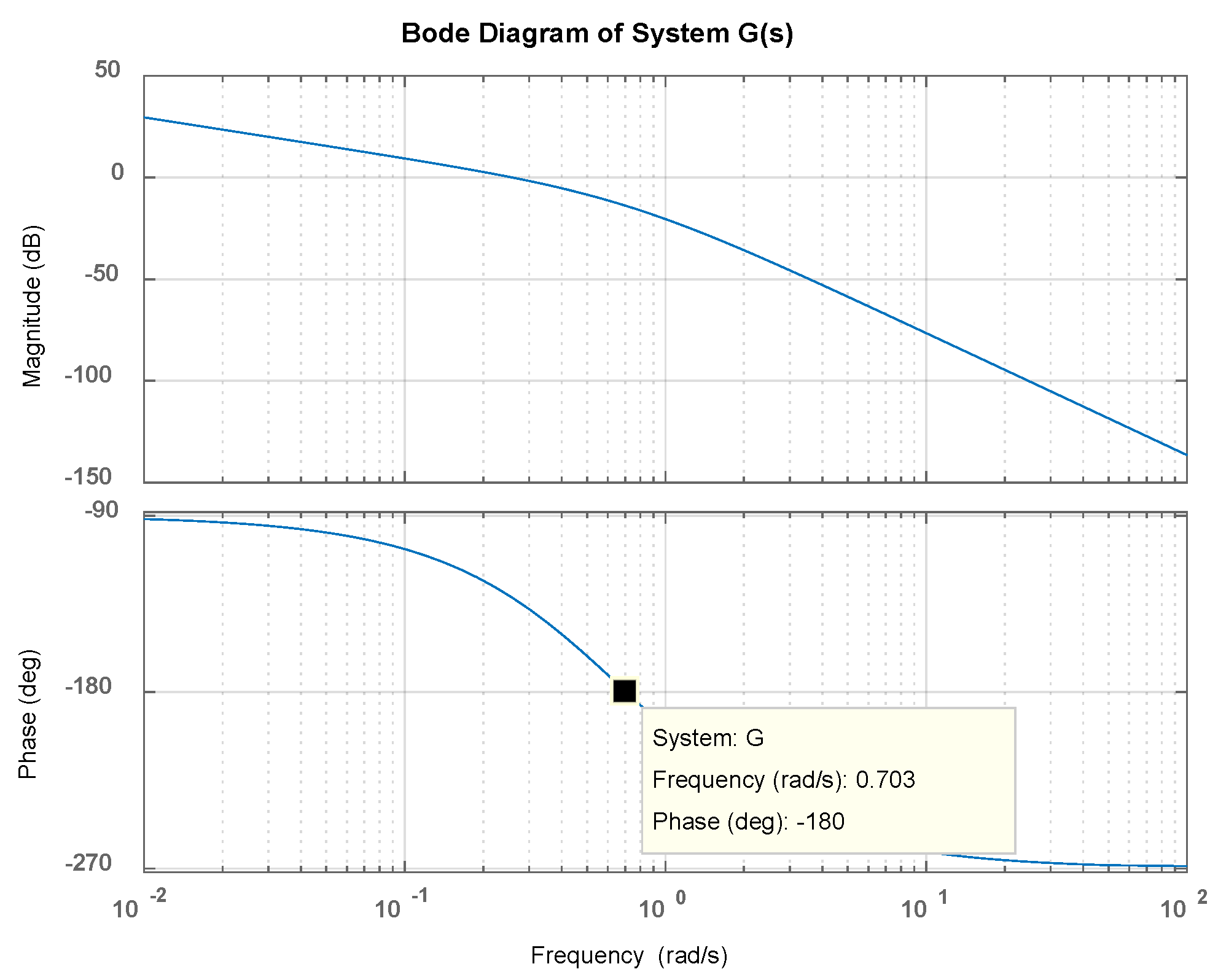
The problem should be reviewed, as it is assumed that the limit cycle takes place in the feedback system with ideal relay nonlinearity. The frequency response of G(s) is shown in Figure 3.

From the Bode plot, it appears that any limit cycle which occurs must be at frequency ‘ω’, where the phase shift is −180°.

The frequency response of the system G(s) in Equation (1) is ω = 0.707. The expression of frequency domain could be found by substituting $\mathrm{s}=\mathrm{j}\mathsf{\omega }$ in the Laplace transform of the plant transfer function. Then, the complex representation of linear transfer function G(jω) is $1.4\angle 1.43$.

In determining the possibility of limit cycle, the critical value of DIDF ${\mathrm{N}(\mathrm{A},\mathrm{B})|}_{\mathrm{c}}$ is calculated by substituting the magnitude of G(jω) into Equation (7), yielding 0.714.

The DIDF of a perfect relay for three common dithers is taken into consideration to analyze the performance of the dithers and their differences. The procedures to compute relay DIDF for each dither are described below [41].

The characteristics of input-output of an ideal relay is given by

$$\mathrm{y}=\mathrm{M}\text{sign}(\mathrm{e})=\{\begin{array}{c}\mathrm{M}; \mathrm{e}>0\\ -\mathrm{M}; \mathrm{e}<0\end{array}$$

(8)

where $\mathrm{e}=\mathrm{A}\sin \mathsf{\omega }\mathrm{t}+\mathrm{B}\sin \mathsf{\beta }\mathrm{t}$, M denotes the value of the parameter of the relay nonlinear element and e is the input of the nonlinearity and β >> ω.

Equation (9) is the original DF with D sin ωt as the input.

$$\begin{array}{l}\mathrm{D}\mathrm{F}=\frac{1}{\mathsf{\pi }\mathrm{A}}{\displaystyle \underset{0}{\overset{2\mathsf{\pi }}{\int }}\mathrm{M}\text{sign}(\mathrm{D}\text{sin} \mathsf{\omega } \mathrm{t})\text{sind} \mathsf{\omega } \mathrm{t}}\\ \mathrm{D}\mathrm{F}=\frac{4\mathrm{M}}{\mathrm{A}}\end{array}$$

(9)

The second integration indicated by Equation (10)

$$\mathrm{N}(\mathrm{A},\mathrm{B})=\frac{1}{2}{\displaystyle \underset{0}{\overset{2\mathsf{\pi }}{\int }}\mathrm{g}(\mathrm{A},\mathrm{B},\mathsf{\varphi })\mathrm{d}\mathsf{\varphi }}$$

(10)

where

$$\mathrm{g}(\mathrm{A},\mathrm{B},\mathsf{\varphi })=\frac{4\mathrm{M}}{\mathsf{\pi }}\left(\frac{1+\frac{\mathrm{B}}{\mathrm{A}}\left(\cos \mathsf{\varphi }\right)}{\sqrt{{\mathrm{A}}^2+{\mathrm{B}}^2+2\mathrm{A}\mathrm{B}\cos \mathsf{\varphi }}}\right)$$

(11)

Substituting Equation (11) in Equation (10) gives

$$\mathrm{N}(\mathrm{A},\mathrm{B})=\frac{4\mathrm{M}}{{\mathsf{\pi }}^2}{\displaystyle \underset{0}{\overset{\mathsf{\pi }}{\int }}\frac{1+\frac{\mathrm{B}}{\mathrm{A}}\cos \mathsf{\varphi }}{\sqrt{{\mathrm{A}}^2+{\mathrm{B}}^2+2\mathrm{A}\mathrm{B}\cos \mathsf{\varphi }}}}$$

(12)

This integral might be evaluated

$$\mathrm{N}(\mathrm{A},\mathrm{B})=\frac{8\mathrm{M}}{{\mathsf{\pi }}^2}\frac{1}{\mathrm{A}+\mathrm{B}}\left[\left(1+\frac{\mathrm{B}}{\mathrm{A}}\frac{{\mathrm{k}}^2-2}{{\mathrm{k}}^2}\right)\mathrm{F}(\mathrm{k})+\left(2+\frac{\mathrm{B}}{\mathrm{A}}\frac{1}{\mathrm{k}}\mathrm{E}(\mathrm{k})\right)\right]$$

(13)

where F(k) is the complete elliptic integral of the first kind and E(k) is the complete elliptic integral of the second kind, with k defining modulus, as shown in Equations (14) and (15).

$$\mathrm{E}(\mathrm{k})=\frac{2\mathrm{E}(\mathrm{k})-\left(1-{\mathrm{k}}^2\right)\mathrm{F}(\mathrm{k})}{1+\mathrm{k}}$$

(14)

$$\mathrm{F}(\mathrm{k})=(1+\mathrm{k})\mathrm{F}(\mathrm{k})$$

(15)

The modulus k is formulated by

$$\mathrm{k}=\frac{\sqrt[2]{\raisebox{1ex}{$\mathrm{B}$}\!\left/ \!\raisebox{-1ex}{$\mathrm{A}$}\right.}}{1+\raisebox{1ex}{$\mathrm{B}$}\!\left/ \!\raisebox{-1ex}{$\mathrm{A}$}\right.}$$

(16)

Equation (13) is valid for all values of A and B when

$$\begin{array}{l}\mathrm{k}=\raisebox{1ex}{$\mathrm{B}$}\!\left/ \!\raisebox{-1ex}{$\mathrm{A}$}\right.; \mathrm{B}<\mathrm{A}\\ \mathrm{k}=\raisebox{1ex}{$\mathrm{A}$}\!\left/ \!\raisebox{-1ex}{$\mathrm{B}$}\right.; \mathrm{B}>\mathrm{A}\end{array}$$

(17)

Substituting Equations (14) through (17) in Equation (13), the following relations are obtained.

$$\mathrm{N}(\mathrm{A},\mathrm{B})=\{\begin{array}{c}\frac{8\mathrm{M}}{\mathsf{\pi }}\mathrm{E}\left(\raisebox{1ex}{$\mathrm{B}$}\!\left/ \!\raisebox{-1ex}{$\mathrm{A}$}\right.\right); \mathrm{B}<\mathrm{A}\\ \frac{8\mathrm{M}}{{\mathsf{\pi }}^2\mathrm{A}}\frac{1}{\mathrm{A}}\left[\mathrm{E}\left(\raisebox{1ex}{$\mathrm{A}$}\!\left/ \!\raisebox{-1ex}{$\mathrm{B}$}\right.\right)-\left(1-\frac{{\mathrm{A}}^2}{{\mathrm{B}}^2}\mathrm{k}\left(\raisebox{1ex}{$\mathrm{A}$}\!\left/ \!\raisebox{-1ex}{$\mathrm{B}$}\right.\right)\right)\right]; \mathrm{A}<\mathrm{B}\end{array}$$

(18)

Equation (18) is the DIDF of ideal relay for sine wave dither signal, as simplified in Equation (19).

$$\mathrm{N}(\mathrm{A},\mathrm{B})=\frac{4\mathrm{M}}{{\mathsf{\pi }}^2}\frac{1}{{\mathrm{A}}^2}\left[(\mathrm{A}-\mathrm{B})\mathrm{K}(\mathrm{k})+(\mathrm{A}+\mathrm{B})\mathrm{E}(\mathrm{k})\right]$$

(19)

The DIDFs of relay for the triangle wave and square wave dithers are given in Equations (20) and (21), respectively.

$$\mathrm{N}(\mathrm{A},\mathrm{B})=\frac{\mathrm{M}}{\mathrm{B}{\mathsf{\pi }}^2}\left(2\mathsf{\gamma }-\sin 2\mathsf{\gamma }\right)+\frac{4\mathrm{M}}{\mathsf{\pi }\mathrm{A}}\cos \mathsf{\gamma }$$

(20)

$$\mathrm{N}(\mathrm{A},\mathrm{B})=\frac{4\mathrm{M}}{\mathsf{\pi }\mathrm{A}}\sqrt{1-\left(\frac{\mathrm{B}}{\mathrm{A}}\right)}$$

(21)

where

$$\mathsf{\gamma }={\sin }^{-1}\left(\frac{\mathrm{B}}{\mathrm{A}}\right)$$

(22)

Here, M is set to be 1. The normalized DIDF $\mathrm{N}(\mathrm{A},\mathrm{B})$ is plotted versus the normalized amplitude A of the input with normalized amplitude B of dither signals as a parameter.

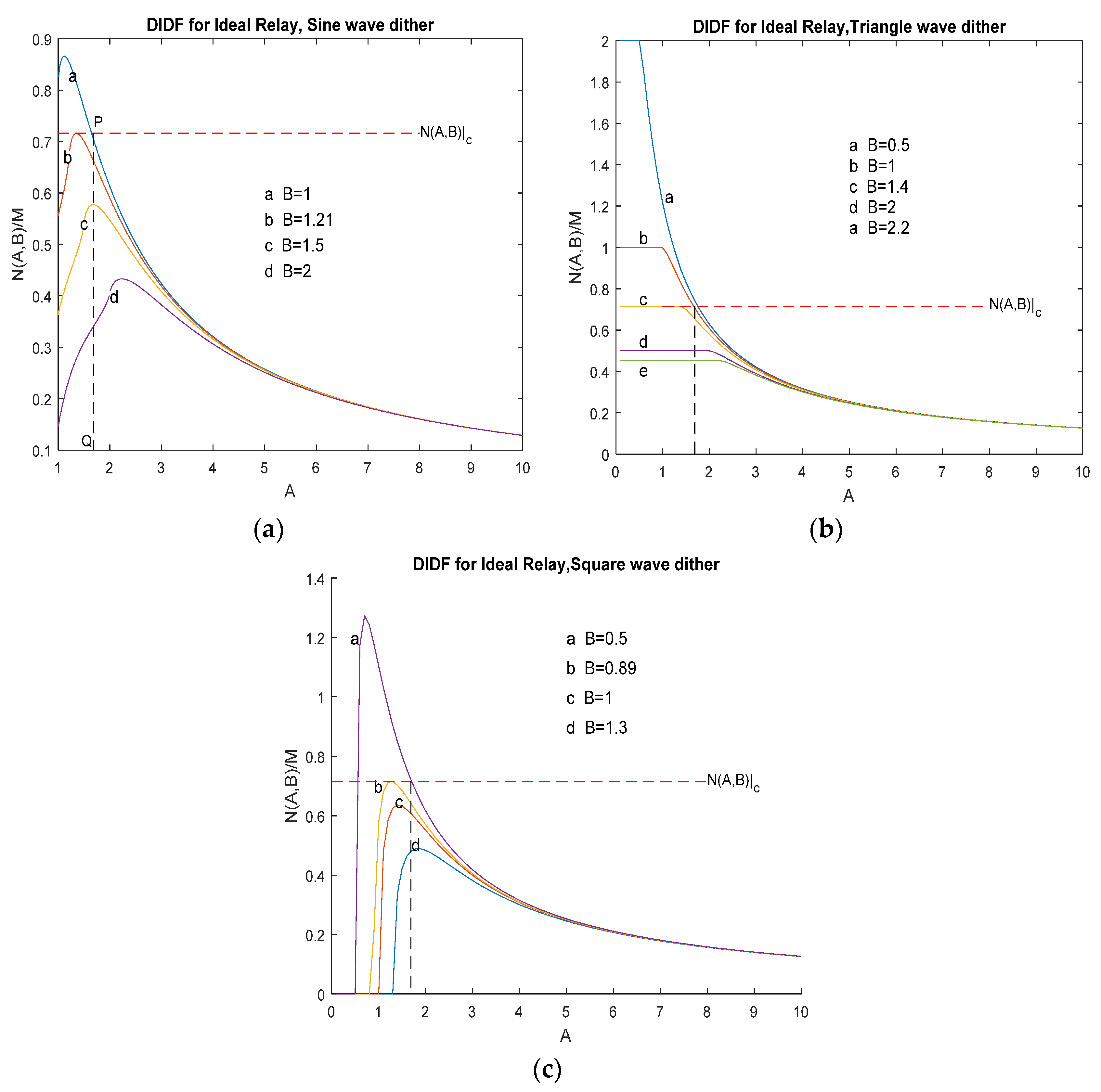
Figure 4a–c for an ideal relay are depicted for the sine wave, triangle, and square wave dithers, respectively.

In these figures, the curves of DIDF are plotted for different amplitudes of dither B as a comparison. A critical line, ${\mathrm{N}(\mathrm{A},\mathrm{B})|}_{\mathrm{c}}$ is also drawn to make it easier when analyzing the limit cycle amplitude. The possibility and amplitude of the limit cycle can be determined by constructing the DIDF curves for a horizontal line of the nonlinearity representing the DIDF critical value or ${\mathrm{N}(\mathrm{A},\mathrm{B})|}_{\mathrm{c}}$.

The limit cycle amplitude is read from the intersection of the ${\mathrm{N}(\mathrm{A},\mathrm{B})|}_{\mathrm{c}}$ line and the DIDF curve. Therefore, the limit cycle amplitude typically is a stabilizing signal or a dither amplitude function. The critical line ${\mathrm{N}(\mathrm{A},\mathrm{B})|}_{\mathrm{c}}$ may not intersect the DIDF curve for a particular dither signal with certain amplitude B. If the entire of the DIDF curve for the amplitude value B lies below the ${\mathrm{N}(\mathrm{A},\mathrm{B})|}_{\mathrm{c}}$ line, then the dither signal with the B value will completely suppress the limit cycles. Otherwise, if the DIDF curve lies above the ${\mathrm{N}(\mathrm{A},\mathrm{B})|}_{\mathrm{c}}$ line, then this dither signal will actually make the system become unstable. In other words, not all the dither signals stabilize the nonlinear system. The selection of suitable dither signal parameter values will have good effects to improve the system performance. For example, as in Figure 4a–c, some curves lie above the critical line ${\mathrm{N}(\mathrm{A},\mathrm{B})|}_{\mathrm{c}}$ and have an intersection, and there are those that lie below the ${\mathrm{N}(\mathrm{A},\mathrm{B})|}_{\mathrm{c}}$ line.

The procedures for finding the limit cycle amplitude are explained below.

Consider the case in Figure 4a. The intersection of the normalized DIDF curve for B = 1 and the critical line ${\mathrm{N}(\mathrm{A},\mathrm{B})|}_{\mathrm{c}}$ at point P represents a possible limit cycle. The amplitude of the limit cycle is read from the projection of the intersection at point P to point S on the abscissa, and the limit cycle amplitude will be 1.69 units. The same means could also be used for relay DIDF for triangle and square dithers in Figure 4b,c. It can be seen that the results display the similarity within Figure 4a.

Figure 4 is a graphical rule to determine the minimum amplitude of the dither signal required to suppress the limit cycle. As plotted in the phase plane of amplitude, it appears obvious that the local lowest point corresponds to the peak of the DIDF curve in Figure 4a–c. Then, set the locus so that it will never cut the locus. This guarantees that the limit cycle will not occur. The required condition is given in Equation (23) or in Equation (24)

$${\mathrm{N}(\mathrm{A},\mathrm{B})|}_{\max }<{\mathrm{N}(\mathrm{A},\mathrm{B})|}_{\mathrm{c}}$$

(23)

or

$$\mathrm{B}\frac{\mathrm{N}(\mathrm{A},\mathrm{B})}{\mathrm{M}}<\frac{{\mathrm{N}(\mathrm{A},\mathrm{B})|}_{\mathrm{c}}}{\mathrm{M}}\mathrm{B}$$

(24)

The peak value ${\mathrm{N}(\mathrm{A},\mathrm{B})|}_{\max }$ for each curve when B = 1 is found from DIDF curves (see Figure 4a–c) for three-wave dithered relay of DIDF, as shown in

Table 1. The peak value of dither signal.

Dither Signal	$\mathbf{The} \mathbf{Peak} \mathbf{Value} \left({\mathbf{N}(\mathbf{A},\mathbf{B})|}_{\mathbf{max}}\right)$
Sine	0.85
Triangle	1
Square	0.64

.

Equation (24) can be simplified to

$${\mathrm{B}}_{\min }>\frac{{\mathrm{N}(\mathrm{A},\mathrm{B})|}_{\max }}{{\mathrm{N}(\mathrm{A},\mathrm{B})|}_{\mathrm{c}}}\mathrm{M}$$

(25)

Substituting M = 1, as stated in the problem, and the peak values of the normalized DIDF curves obtained earlier in Equation (25) yield the minimum values of dither amplitudes for each dither, which are given in

Table 2. The minimum value of dither amplitude.

Dither Signal	$\mathbf{The} \mathbf{Minimum} \mathbf{Value} \mathbf{of} \mathbf{Dither} \mathbf{Amplitude} \left({\mathbf{B}}_{\mathbf{min}}\right)$
Sine	>1.2
Triangle	>1.4
Square	>0.89

below.

As can be seen, a smaller square wave dither amplitude is required to quench the limit cycle than those of triangle or sine wave dithers. The maximum $\mathrm{N}{(\mathrm{A},\mathrm{B})}_{\max }$ displays that the peak value of the normalized DIDF curve when the amplitude of dither chosen to be the minimum point is present in the critical line ${\mathrm{N}(\mathrm{A},\mathrm{B})|}_{\mathrm{c}}$. Here, there is no intersection between the critical line ${\mathrm{N}(\mathrm{A},\mathrm{B})|}_{\mathrm{c}}$ and the DIDF curve for the minimum B. Therefore, if the amplitude of dither B is greater than B_min, then no limit cycle will exist.

3. Results and Discussion

In this section, the example of a nonlinear feedback system containing a perfect relay nonlinear element exhibit in Figure 1 will be examined under a simulation using a digital computer. Matlab-Simulink 2016b package is used as a simulation tool to illustrate and verify the analysis method, which was developed in the previous section. In this case, the simulation software is running on a laptop with the specifications as follows: (1) Intel(R) Core(TM) i5-4200U Processor @ 1.60 GHz, (2) 4096 MB RAM, (3) Windows 7 Professional 64-bit Operating System.

Figure 5 shows the Simulink block diagram of the relay feedback system. It could be seen that the linear part of the system is low pass and assumes that the input of the relay nonlinearity is the sum of a dither signal and fundamental sinusoidal component. The frequency of the dither signal chosen is ten times of ω = 0.707.

In this simulation, the input used is a unit step. The dither signal is introduced into the system before the nonlinear element. The actual signal output will be monitored using a scope. Three different types of dither signals were used in simulation tests of the relay control system: sine, triangle, and square waves.

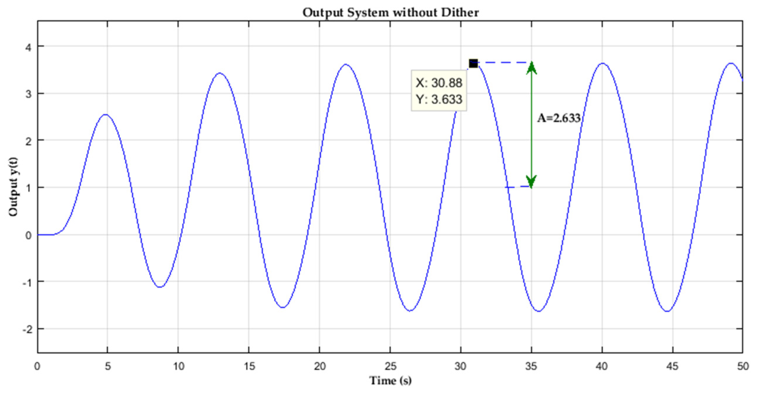
The limit cycle amplitude which was calculated using the DIDF method in the previous section for a sine wave dither amplitude of B = 1 will be verified using the Simulink program. The output system without dither injection was also displayed to compare the effect of dither introduced. The simulation results of the system with no dither signal showed that the limit cycle appears in system output with a 2.633-unit amplitude, as depicted in Figure 6.

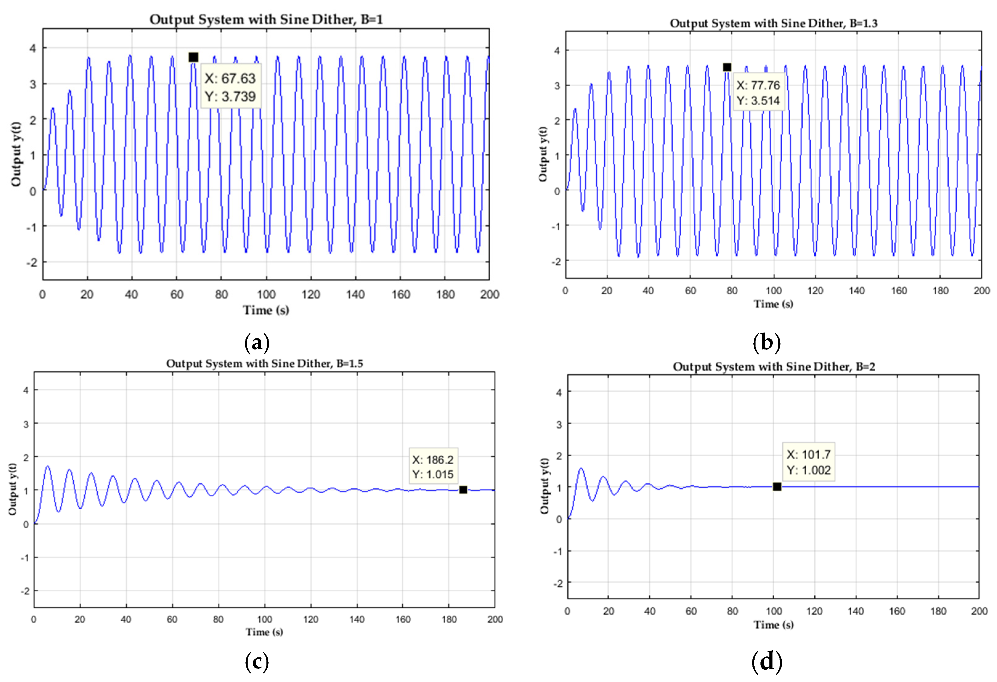
The next consideration should be put on the amplitude of sustained oscillation in Figure 6 when a sine wave dither with amplitude of 1 is added into the system. The 2.739-unit amplitude of the limit cycle is read from the simulation result. Compared to the calculation result before, it is not exactly the same as these two results. However, the DIDF method is just an approximation. All the simulation results for different amplitudes and the same frequency of dither B for three shapes of dither signals are shown in Figure 7, Figure 8 and Figure 9. In Figure 7, for sine wave dither simulation results, it is interesting to see that when B = 1.5 unit, the dither signal starts to turn the limit cycle off. We also notice that the limit cycle amplitude decreased from 3.7 to 0.002 units when B = 2.

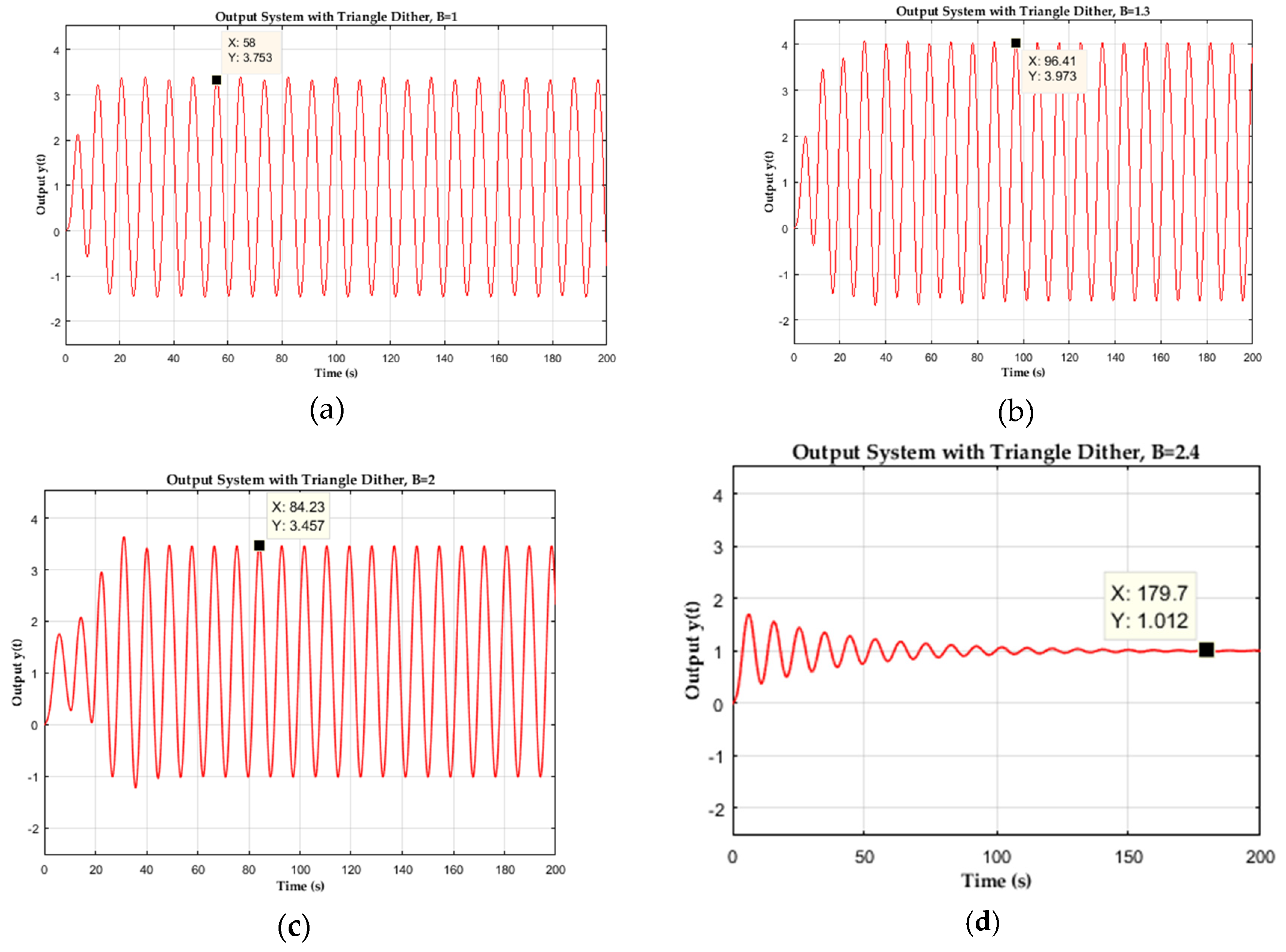
Considering the ideal relay DIDF curve for triangle wave dither signal (Figure 8), again, the limit cycle presents a gradual decrease with respect to the dither amplitude. Meanwhile, it shows that the limit cycle can be removed when the dither amplitude is 2.4 units. This amplitude value is greater than that of the sine wave dither. This fact corroborates the previous analysis.

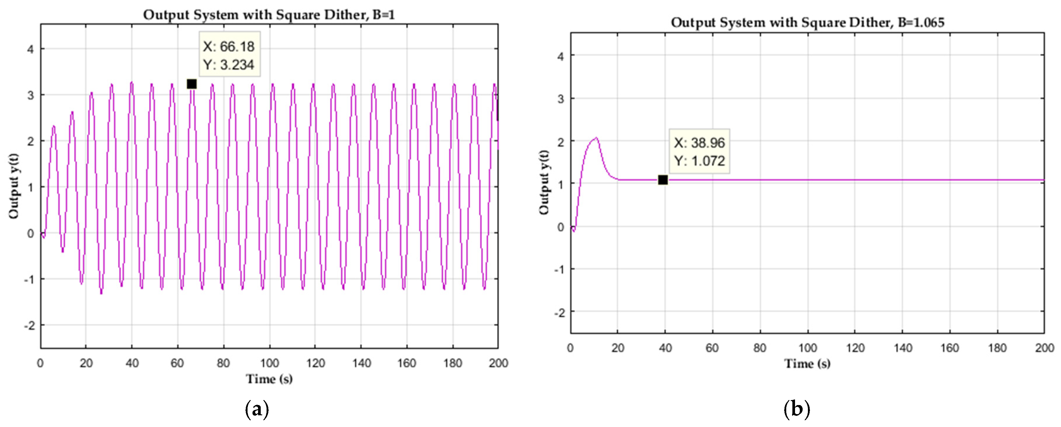
Finally, Figure 9 depicts the effect of square wave dither injection to quench limit cycle. The minimum amplitude required should be at least 1.065 units. Even though all the simulation results showed that the minimum amplitude of the dither signal is not exactly the same as those obtained through the calculation of the analyses, generally, these results clearly validate the theoretical investigation in the previous section.

Table 3. The results of analytical and the simulation studies for the relay feedback system.

Dither Shape	Predicted		Simulation
	A	${\mathbf{B}}_{\mathbf{min}}$	A	${\mathbf{B}}_{\mathbf{min}}$
Sine	1.69	>1.22	2.739	≥1.5
Triangle	1.69	>1.4	2.753	≥2.4
Square	1.69	>0.89	2.234	≥1.065

shows a summary of this work from both analytical and simulation studies.

4. Conclusions and Future Works

The main finding of this work is the dithering technique with a suitable high-frequency signal to suppress the limit cycle oscillation of the control system with one nonlinearity component. The DIDF method and practical guidelines have been presented to predict the limit-cycle amplitude and design the dither signal amplitude. These works were verified on a nonlinear feedback loop system with a perfect relay nonlinearity element using Matlab-Simulink simulation software. It has been shown that, for controlling a servo feedback loop system with an ideal relay nonlinearity element, the sustained oscillation or limit-cycle occurring in output can be quenched using the dithering injection strategy. The simulation results illustrate the effect of changing the dither signal parameters, shape and amplitude in a controller design for the system under study. It was found that dither is a function of amplitude, which means that dither amplitude had effects on the smoothed system. Here, the square dither had the minimum amplitude needed to narrow the nonlinear system, compared to triangle and sine wave dither. Therefore, it is necessary to do the analytical calculation under the DIDF term to find the correct dither amplitude and consider the choice of dither shape in the dithering method.

Future works have to be carried out in a practical experiment to investigate the application of the purposed technique, such as in the DC Servo Motor system which has backlash and saturation with dead zone nonlinearities. The self-oscillations or limit cycles that occur in this servo system will be investigated using the DIDF approach. Then, the dithering technique will be applied to suppress the limit cycle.

References

- Huang, B.; Yap, C. An algorithmic approach to small limit cycles of nonlinear differential systems: The averaging method revisited. J. Symb. Comput. 2020. [Google Scholar] [CrossRef]
- Yang, J. Limit cycles appearing from the perturbation of differential systems with multiple switching curves. Chaos Solitons Fractals 2020, 135, 109764. [Google Scholar] [CrossRef] [Green Version]
- Balajewicz, M.; Dowell, E. Reduced-order modeling of flutter and limit-cycle oscillations using the sparse Volterra series. J. Aircr. 2012, 49, 1803–1812. [Google Scholar] [CrossRef]
- Slotine, J.-J.E.; Li, W. Nonlinear system analysis. In Applied Nonlinear Control; Prentice Hall: Englewood Cliffs, NJ, USA, 1991; Volume 199. [Google Scholar]
- Hayes, R.; Marques, S.P. Prediction of limit cycle oscillations under uncertainty using a harmonic balance method. Comput. Struct. 2015, 148, 1–13. [Google Scholar] [CrossRef] [Green Version]
- Shukla, H.; Patil, M.J. Controlling limit cycle oscillation amplitudes in nonlinear aeroelastic systems. J. Aircr. 2017, 54, 1921–1932. [Google Scholar] [CrossRef] [Green Version]
- Zhang, G.; Wu, Z. Approximate limit cycles of coupled nonlinear oscillators with fractional derivatives. Appl. Math. Model. 2020, 77, 1294–1309. [Google Scholar] [CrossRef]
- Al-Moqbali, M.K.; Al-Salti, N.S.; Elmojtaba, I.M. Prey-predator models with variable carrying capacity. Mathematics 2018, 6, 102. [Google Scholar] [CrossRef] [Green Version]
- Denimal, E.; Sinou, J.-J.; Nacivet, S. Generalized Modal Amplitude Stability Analysis for the prediction of the nonlinear dynamic response of mechanical systems subjected to friction-induced vibrations. Nonlinear Dyn. 2020, 100, 1–24. [Google Scholar] [CrossRef]
- Taylor, J.H. Describing functions. In Electrical Engineering Encyclopedia; John Wiley & Sons: New York, NY, USA, 1999. [Google Scholar]
- Zare, S.; Tavakolpour-Saleh, A.; Sangdani, M. Investigating limit cycle in a free piston Stirling engine using describing function technique and genetic algorithm. Energy Convers. Manag. 2020, 210, 112706. [Google Scholar] [CrossRef]
- Xia, Y.; Laera, D.; Jones, W.P.; Morgans, A.S. Numerical prediction of the Flame Describing Function and thermoacoustic limit cycle for a pressurised gas turbine combustor. Combust. Sci. Technol. 2019, 191, 979–1002. [Google Scholar] [CrossRef]
- Maraini, D.; Nataraj, C. Nonlinear analysis of a rotor-bearing system using describing functions. J. Sound Vib. 2018, 420, 227–241. [Google Scholar] [CrossRef]
- Yang, Z.; Li, H.; Liu, C.; Ding, Y.; Zhang, B. Accurate modeling and stability analysis for chaotic PWM boost converters based on describing function method. In Proceedings of the IECON 2019—45th Annual Conference of the IEEE Industrial Electronics Society, Lisbon, Portugal, 14–17 September 2019; pp. 1585–1590. [Google Scholar]
- Namadchian, Z.; Zare, A. Stability analysis of dynamic nonlinear interval type-2 TSK fuzzy control systems based on describing function. Soft Comput. 2020, 24, 1–14. [Google Scholar] [CrossRef]
- Shukla, H.; Patil, M.J. Nonlinear state feedback control design to eliminate subcritical limit cycle oscillations in aeroelastic systems. Nonlinear Dyn. 2017, 88, 1599–1614. [Google Scholar] [CrossRef]
- Girija, S.; Narayanasamy, S.; Kurian, T. Method to eliminate the limit cycle oscillation for digitally controlled DC–DC converter using reduced state Kalman filter. IET Power Electron. 2016, 9, 2445–2452. [Google Scholar] [CrossRef]
- Kumar, A.; Ali, S.F.; Friswell, M.I.; Arockiarajan, A. Creation and stabilization of limit cycles in chaotic attractors through closure of orbits. In Proceedings of the 11th Asian Control Conference (ASCC), Gold Coast, Australia, 17–20 December 2017; pp. 653–658. [Google Scholar]
- Antonio-Cruz, M.; Hernández-Guzmán, V.M.; Silva-Ortigoza, R.; Silva-Ortigoza, G. Implementation of a controller to eliminate the limit cycle in the inverted pendulum on a cart. Complex 2019, 2019, 13. [Google Scholar] [CrossRef]
- Oldenburger, R.; Nakada, T. Signal stabilization of self-oscillating systems. IRE Trans. Autom. Control 1961, 6, 319–325. [Google Scholar] [CrossRef]
- Yang, H.; Tao, W.; Zhang, Z.; Zhao, S.; Yin, X.; Zhao, H. Reduction of the influence of laser beam directional dithering in a laser triangulation displacement probe. Sensors 2017, 17, 1126. [Google Scholar] [CrossRef] [Green Version]
- Duan, Y.; Chen, T.; Chen, D. Low-cost dithering generator for accurate ADC linearity test. In Proceedings of the 2016 IEEE International Symposium on Circuits and Systems (ISCAS), Montreal, QC, Canada, 22–25 May 2016; pp. 1474–1477. [Google Scholar]
- Tao, Y.; Li, S.; Zhou, G.; Lin, J. Mechanical dither control optimization for laser gyro with total reflection prisms. In Proceedings of the 2017 24th Saint Petersburg International Conference on Integrated Navigation Systems (ICINS), Saint Petersburg, Russia, 29–31 May 2017; pp. 1–7. [Google Scholar]
- Zhang, S.; Li, T.; Jin, L.; Yang, J.; He, L.; Lin, F. A 11-bit 1.2 V 40.3 μW SAR ADC with Self-Dithering Technique, 2016 IEEE MTT-S International Wireless Symposium (IWS); IEEE: New York, NJ, USA, 2016; pp. 1–4. [Google Scholar]
- Zhu, H.; Fujimoto, H. Suppression of current quantization effects for precise current control of SPMSM using dithering techniques and Kalman filter. IEEE Trans. Ind. Inform. 2014, 10, 1361–1371. [Google Scholar]
- Wang, X.; Suh, C.S. Nonlinear time-frequency control of PM synchronous motor instability applicable to electric vehicle application. Int. J. Dyn. Control 2016, 4, 400–412. [Google Scholar] [CrossRef]
- Behera, R.K.; Das, S.P. High performance induction motor drive: A dither injection technique. In Proceedings of the 2011 International Conference on Energy, Automation and Signal, Bhubaneswar, India, 28–30 December 2011; pp. 1–6. [Google Scholar]
- Behera, R.; Das, S. Improved direct torque control of induction motor with dither injection. Sadhana 2008, 33, 551–564. [Google Scholar] [CrossRef]
- Kadjoudj, M.; Taibi, S.; Golea, N.; Benbouzid, M. Modified direct torque control of PMSM drives using dither signal injection and non-hysteresis controllers. Electromotion 2006, 13, 262–270. [Google Scholar]
- Chang, S.-C. Quenching chaos of a magnetically levitated system based on dither signals. Appl. Math. Comput. 2013, 222, 539–547. [Google Scholar] [CrossRef]
- Chang, S.-C. Stability analysis, routes to chaos, and quenching chaos in electromechanical valve actuators. Math. Comput. Simul. 2020, 177, 140–151. [Google Scholar] [CrossRef]
- Lue, Y.-F.; Chang, S.-C. Non-linear dynamics and control of an automotive suspension system based on local and global bifurcation analysis. Int. J. Veh. Auton. Syst. 2017, 13, 340–359. [Google Scholar] [CrossRef]
- Gibson, J.; Sridhar, R. A new dual-input describing function and an application to the stability of forced nonlinear systems. IEEE Trans. Appl. Ind. 1963, 82, 65–70. [Google Scholar] [CrossRef]
- Chen, S.-C.; Tsai, H.-H. The Performance of different dither signals in nonlinear systems. Mod. Phys. Lett. B 2009, 23, 2507–2520. [Google Scholar] [CrossRef]
- Raafat, S.M.; Ali, S.S. The selection of dither signal in extremum seeking control of 3 DOF helicopter system. In Proceedings of the Zaytoonah University International Engineering Conference on Design and Innovation in Sustainability, Amman, Jordan, 13–15 May 2014; pp. 13–15. [Google Scholar]
- West, J.; Douce, J.; Livesley, R. The dual-input describing function and its use in the analysis of non-linear feedback systems. Proc. IEEE Part B Radio Electron. Eng. 1956, 103, 463–473. [Google Scholar] [CrossRef]
- Kasi, V.R.; Majhi, S.; Gogoi, A.K. Estimation of stable FOPDT and SOPDT process using dual input describing function. In Proceedings of the 11th International Conference on Industrial and Information Systems (ICIIS), Roorkee, India, 3–4 December 2016; pp. 810–814. [Google Scholar]
- Choe, Y.W. Performance Improvement for PID Controllers by using Dual-Input Describing Function (DIDF) Method. Trans. Korean Inst. Electr. Eng. 2011, 60, 1741–1747. [Google Scholar] [CrossRef] [Green Version]
- Choe, Y.W. Tuning PID controllers for unstable systems with dead time based on dual-input describing function method. In AETA 2015: Recent Advances in Electrical Engineering and Related Sciences; Springer: Berlin, Germany, 2016; pp. 427–439. [Google Scholar]
- Brito, A.G. Computation of multiple limit cycles in nonlinear control systems-a describing function approach. J. Aerosp. Technol. Manag. 2011, 3, 21–28. [Google Scholar] [CrossRef]
- Welford, G.D. Dual input describing functions. In Army Missile Research Development and Engineering Lab Redstone Arsenal al Guidance and Control Directorate; Army Missile Command: Redstone Arsenal, AL, USA, 1969. [Google Scholar]
Figure 1.
Nonlinear system with dither applied.
Figure 2.
Nonlinear system.
Figure 3.
Frequency Response of the linear plant.
Figure 4.
DIDF curve for Ideal Relay, (a) Sine wave dither, (b) Triangle wave dither, (c) Square wave dither.
Figure 5.
Simulink block diagram of the relay control system with dither injection.
Figure 6.
Closed-loop step response without any Dither signal injection. The amplitude of the limit cycle is 2.633 units.
Figure 7.
Closed-loop step response with Sine wave dither injection, (a) with dither amplitude B = 1, (b) B = 1.3, (c) B = 1.5, and (d) B = 2.
Figure 8.
Closed-loop step response with Triangle wave dither injection, (a) with dither amplitude B = 1, (b) B = 1.3, (c) B = 2, (d) B = 2.4
Figure 9.
Closed-loop step response with Square wave dither injection, (a) with dither amplitude B = 1, (b) B = 1.065. When B = 1, the limit cycle amplitude is 2.234 units.