Design of Constrained Robust Controller for Active Suspension of In-Wheel-Drive Electric Vehicles
by
Xianjian Jin
1,2,*, 
Jiadong Wang
1,
Shaoze Sun
1,
Shaohua Li
3,*,
Junpeng Yang
1 and
Zeyuan Yan
1 1
School of Mechatronic Engineering and Automation, Shanghai University, Shanghai 200072, China
2
Shanghai Key Laboratory of Intelligent Manufacturing and Robotics, Shanghai University, Shanghai 200072, China
3
State Key Laboratory of Mechanical Behavior and System Safety of Traffic Engineering Structures, Shijiazhuang Tiedao University, Shijiazhuang 050043, China
*
Authors to whom correspondence should be addressed.
Mathematics 2021, 9(3), 249; https://doi.org/10.3390/math9030249
Submission received: 27 December 2020
/
Revised: 16 January 2021
/
Accepted: 24 January 2021
/
Published: 27 January 2021
Abstract
:This paper presents a constrained robust H∞ controller design of active suspension system for in-wheel-independent-drive electric vehicles considering control constraint and parameter variation. In the active suspension system model, parameter uncertainties of sprung mass are analyzed via linear fraction transformation, and the perturbation bounds can be also limited, then the uncertain quarter-vehicle active suspension model where the in-wheel motor is suspended as a dynamic vibration absorber is built. The constrained robust H∞ feedback controller of the closed-loop active suspension system is designed using the concept of reachable sets and ellipsoids, in which the dynamic tire displacements and the suspension working spaces are constrained, and a comprehensive solution is finally derived from H∞ performance and robust stability. Simulations on frequency responses and road excitations are implemented to verify and evaluate the performance of the designed controller; results show that the active suspension with a developed H∞ controller can effectively achieve better ride comfort and road-holding ability compared with passive suspension despite the existence of control constraints and parameter variations.
1. Introduction
Emerging in-wheel-motor-driven electric vehicles (IWMD-EV) have appeared as promising vehicle architectures in terms of several advantages, such as less fuel consumption and environmental pollution, clean energy with electrified power sources, and advanced vehicle dynamics control [1,2]. IWMD-EV uses hub motors to directly drive four wheels by replacing the mechanical transmission link with X-by-wire systems; it is easier to realize independent control and rapid response of each wheel torque, which provide more flexibilities and traffic mobility for the vehicle dynamic control (VDC) system. According to the advantages of advanced vehicle architectures, numerous studies on VDC system, such as traction control system (TCS), active steering system (AFS), direct yaw moment control (DYC), regenerative braking system (RBS), and so forth, have been conducted for improving vehicle handling comfort, vehicle stability, and active safety for IWMD-EV in recent years [3,4,5,6,7,8,9,10,11,12].
Although the aforementioned research achievements were successful, most research papers are concerned with lateral and longitudinal VDC systems, and vertical vibration control of active suspension system of IWMD-EV is seldom tackled [13,14,15,16,17]. In practice, when the new vehicle topology structure for IWMD-EV is brought forward, the active suspension system with in-wheel-motor also changes particularly, in which motor, the wheel hub, and speed reducer are mounted and integrated; it causes the increased unsprung mass of IWMD-EV so that vehicle ride comfort will deteriorate and even road holding ability and safety will be probably reduced. Hence, advanced IWM-based suspension system topology with a dynamic-damper mechanism needs to be developed. Moreover, active control for the active suspension system of IWMD-EV should be particularly concerned.
Robust control technology has been shown to possess the ability to deal with the system modeling uncertainties and system external disturbances [1,4,7,12,18,19,20,21]. Some robust controllers have been applied in active suspension dynamics [22,23,24,25,26,27,28,29,30], such as mixed H∞/GH2 control, fuzzy control, sliding mode control, and other nonlinear adaptive robust methods. For instance, the H∞/GH2 static-output feedback controller of vehicle suspension is proposed for optimizing the ride-comfort performance by utilizing advanced genetic algorithms; it can find the solution of feedback controller, taking advantage of natural genetics search mechanism in [23]. The work in [24] presented a multi-objective control of active vehicle suspension with wheelbase preview information where disturbances for the front wheel are employed as a preview at the rear wheel, and the cone complementarity linearization solution is also derived. The research [26] developed an integrated VDC system to improve vehicles handling stability and safety performance by coordinating AFS and active suspension; the designed gain-scheduling state-feedback H∞ controller is based on the lateral stability region described from the phase plane approach. A quasi-linear parameter-varying (qLPV) active suspension model-based predictive control algorithm is introduced in [27] to enhance the comfort of passengers with semi-active suspension. In [28], a new adaptive fuzzy control scheme for active suspension systems subject to control input time delay and unknown nonlinear dynamics is studied; the Lyapunov–Krasovskii functional and predictor-based compensation scheme is constructed in this adaptive framework. The adaptive sliding mode control scheme with strong robustness for half-car active suspension is reported in [29]; it is concerned with model uncertainty, time-varying parameter, pavement roughness excitation by applying the multivariable nonlinear control solution. A continuous saturated controller using smooth saturation functions for an active suspension system is designed, in which nonlinear uncertainties, unknown road excitations, and bounded disturbances are considered by employing the advantages of the robust integral of the sign of the error (RISE) control technique to improve the ride comfort [30].
It is worth noting that, different from published achievements in literature, e.g., [22,23,24,25,26,27,28,29,30], the main contribution in this work is to explore the control strategy of active suspension system for IWMD-EV rather than traditional car suspension. For IWMD-EV, the motor, the wheel hub, and speed reducer are mounted and integrated so that vehicle ride comfort will deteriorate. Besides, designing a constrained robust H∞ controller for such an active suspension system of IWMD-EV is seldom. We consider that the uncertain quarter-vehicle active suspension model of IWMD-EV in Figure 1 is different from traditional car suspension; thus, these theoretical results derived from constrained robust H∞ controller is particular in this study. Therefore, this paper intends to design a constrained robust H∞ controller for active suspension system to improve ride comfort and road-holding ability of IWMD-EV. The remainder of the article is organized as follows. In Section 2, an uncertain active suspension model considering parameter variations is presented. Section 3 designs the constrained robust H∞ controller for vehicle active suspension system. In Section 4, simulations about random and bump responses are employed to test the developed controller. Finally, conclusions are given in Section 5.
2. Active Suspension System Model
Because the main research objective is to design a control strategy of the active suspension system IWMD-EV, the system model is not essentially concerned with vehicle lateral dynamics (sideslip, yaw, roll) behavior. We consider the following assumptions: IWMD-EV is independently actuated with in-wheel motors, and the active suspension system is integrated with the IWM absorber. Assume that the vertical motion of the active suspension system is only considered, and other vehicle motions, such as pitch and roll motions, are neglected. As shown in Figure 1, the schematic configuration, the application model, and physical structure for quarter-car active suspension with suspended IWM absorber (ASS) are depicted, in which in-wheel motor is connected with dynamic vibration mechanism [13,14]. Note that if IWM absorber cannot be considered in the active suspension system, i.e., the in-wheel motor is directly connected with the wheel, the active suspension presents the new vehicle topology structure, namely active suspension with centralized IWM (ASC). The reason being that the quarter-car active suspension model, despite its simplicity, features the main characteristics of interest to control strategy development and suspension performance assessment. It is worth noting that the quarter-car active suspension model is not suitable to study and simulate vehicle handling responses and stability subjected to various steering excitations. The quarter-car active suspension model can be established as
where ms, mt, and mh represent the sprung mass, the wheel mass, and motor mass, respectively. Ks and Cs are suspension stiffness and the suspension damping coefficient, respectively. Kh and Ch denote the stiffness and damping coefficient of the damping system between the motor and the unsprung mass, respectively. Kt is tire stiffness. Zs, Zh, Zt, and Zg stand for the vertical displacement of the vehicle body, wheel, motor, and road, respectively.
In this suspension system, the vehicle body mass is considered as an uncertain parameter, and the nominal value and relative variation can be described as:
where represents the nominal value of the parameter, represents the perturbation of the uncertain parameter with bound .
In order to facilitate the analysis of structural uncertainty, the parameter uncertainties can be transformed into
where denotes linear fractional transformation (LFT), and its input and output relationship is shown in Figure 2.
We define the state variables of the quarter-car suspension system as follows:
The magnitude of body acceleration can be selected to represent certainly ride comfort, so we define performance output as
Considering the steering stability of the vehicle, it is required that the tires of the vehicle cannot leave the road when the vehicle is driving, and the dynamic load between the tire and the road should be less than the static load, that is
Meanwhile, due to the limitation of the suspension mechanical structure, the suspension working space should not be too large to avoid collision with the limit
where the maximum suspension working space should be limit to Smax = 0.08 m.
In addition, the output power of the force generated by a suspension can be limited as
and then, the constraint output variables can be defined as
When we combine the above derivations and equations, the state space representation of the open-loop suspension model with parameter uncertainties and constraints is derived as
where
3. Constrained Robust H∞ Controller Design
In order to enhance the vehicle’s ride comfort, the road-holding performance of IWMD-EV, our main control goal is to guarantee robust stability and performance for a closed-loop system of active suspension. Hence, we are interested in the state-feedback control law for constrained H∞ controller system.
Substituting (13) into the vehicle active suspension system (12) gives the state-space representation of the vehicle closed-loop system as
where
where x, u, and w are the state vector, the control input, and the disturbance, respectively. z1, z2 are the performance output and the constraint output, respectively. p and q are the input and output of the uncertainties, respectively. The block diagram of the controller structure is shown in Figure 3. It is worth noting that these states in the controller are assumed to be estimated or measured online by designing observers or using advanced sensors [31,32].
In this paper, the following theorem presents the main design process of the robust state-feedback constrained H∞ controller with a defined performance measure.
Theorem 1.
For a given index α > 0, the state-feedback constrained H∞ controller in (13) exists such that the closed-loop system in (14) is internally stable and possesses H∞ norm from the disturbance w to the performance output z for less than γ if there is an optimal solution for bounded disturbance energy ε to satisfy the following conditions:
where
Proof.
For the closed-loop system (14), we define the Lyapunov function as
When we take the time derivative V(x) for the system (14), then we can obtain dissipation inequality as follows:
The integral dissipation inequality of the system with respect to time gives
Owing to , the inequality can be rewritten as
Substituting (14) into the above inequality results in
where
Equation (14e) is equivalent to
and then, we have
It is also equivalent to
where
Using S-procedure for Equations (20) and (21), there exists P > 0, , , …, such that:
For any , the sufficient condition for the above equation to hold is
where
It can be rewritten as
Defining , and then by applying the Schur complement, we obtain
That is
We use the Schur complement again,
Making a congruence transformation with for conditions (29), and then the condition (29) becomes the condition (30) after using these defined matrices .
Particularly, we define constrained condition with the ellipsoid as
Assuming that the state trajectory of the system (14) is in this ellipsoid, we use Cauchy–Schwarz inequality [33]
For all and , the system output meets the constraint requirements
For , , utilizing S-procedure for Equations (31) and (32), we can obtain the following, if there exists and diagonal matrix
When we define , for any and , the above equation can be derived as
It can be rewritten as
Making a congruence transformation with for conditions (36), we have the following form through defined matrices .
and then, substituting , , , in condition (30) and condition (37), when we define new , then the conditions in (16) can be obtained, hence the proof is accomplished. □
Remark 1.
Note that it is feasible to obtain the best performance by applying this constrained H∞ control strategy for each motor of the quarter-car active suspension, whereas global coordination or multi-objective optimization is necessary between the controllers when the full-car suspension, seat suspension, and driver body model is used and integrated because the main control objectives for integrated suspension system are to reduce the vibration of human body and vehicle as well as ensure vehicle handling and stability.
4. Simulation and Analysis
To verify and evaluate the performance of the designed controller, two kinds of road excitations consisting of random road and bump road are implemented for passive suspension, active suspension with constrained H∞ controller in MATLAB/Simulink environment, and the parameters of suspension simulation are listed in Table 1. When the obtained H∞ performance γ by using Theorem is 8.2890 for active suspension with suspended IWM absorber, the corresponding M, N, Q, Y can be calculated as
The corresponding constrained H∞ controller gains are
4.1. Frequency Responses
Frequency responses of closed-loop passive suspension and active suspension systems with constrained robust H∞ controller consisting of body acceleration (BA), suspension working space (SWS), dynamic tire displacement (DTD) are shown in Figure 4, Figure 5 and Figure 6. The constrained robust H∞ controller produces a good improvement on body acceleration and dynamic tire displacement of suspension in the frequency range between 100 and 101 Hz, which indicates that the designed constrained H∞ controller possesses better passenger comfort and road-holding ability.
4.2. Random Road Excitation
Firstly, random road vibration with C-level road irregularities is considered as random excitation; three random road responses—body acceleration (BA), suspension working space (SWS), dynamic tire displacement (DTD)—are illustrated in Figure 7, Figure 8 and Figure 9. It can be seen that active suspension with constrained H∞ controller generates a good improvement on the BA and DTD responses compared with the passive suspension; it even exhibits more than 65% lower BA responses than the passive suspension, which indicates that the vehicle passenger comfort and road holding ability performances can be improved by the H∞ controller. Note that suspension working space of active suspension with H∞ controller shows larger values than that of passive suspension; the reason for this phenomenon is that passenger comfort is always conflicted with SWS in suspension controller design.
4.3. Bump Road Excitation
The second road profile is an isolated bump road excitation, and it can be described as
where v is vehicle forward velocity, L and h are the length and the height of the bump, respectively. Here, we define v = 18 m/s, L = 5 m, and h = 0.08 m.
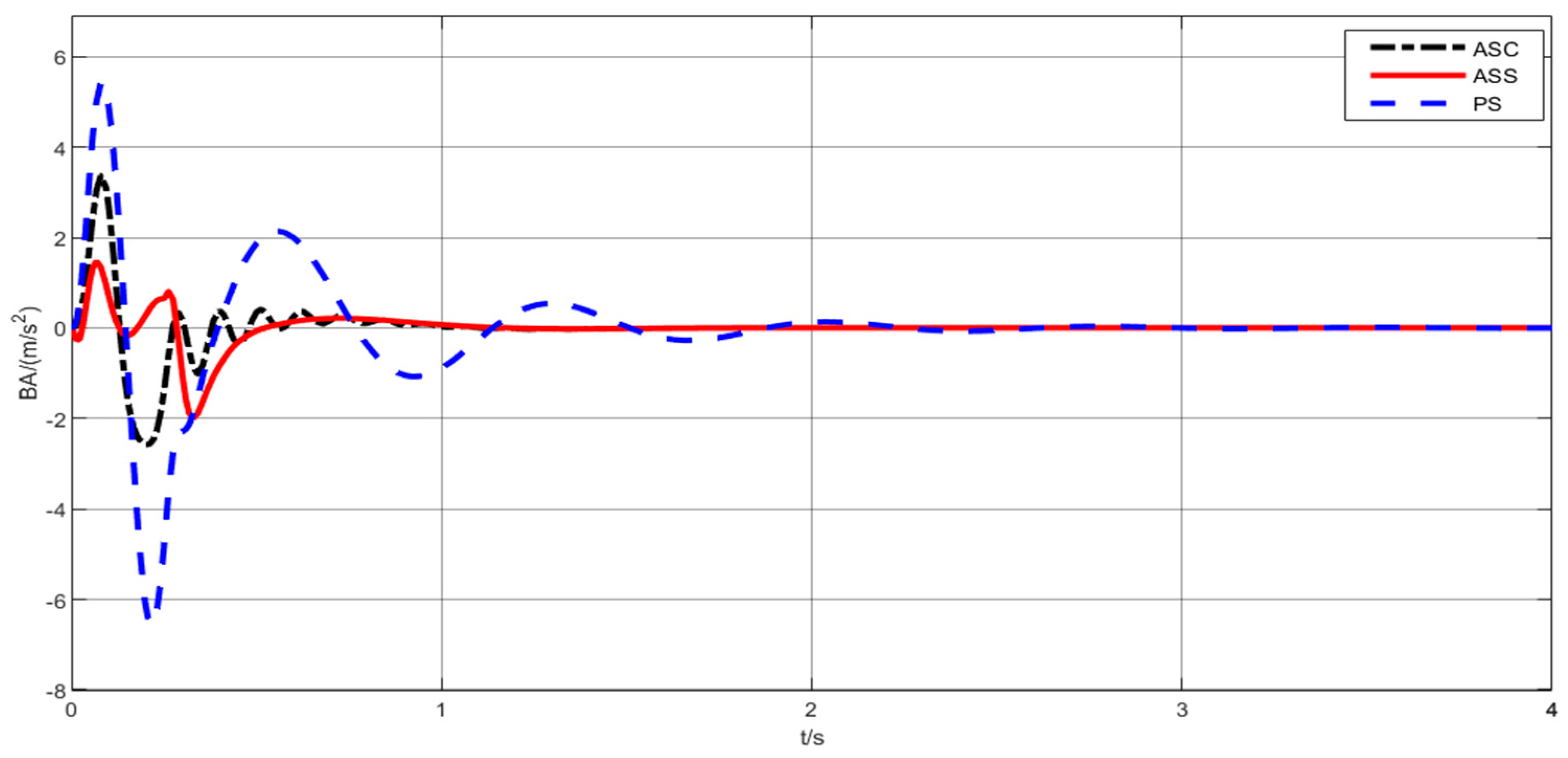
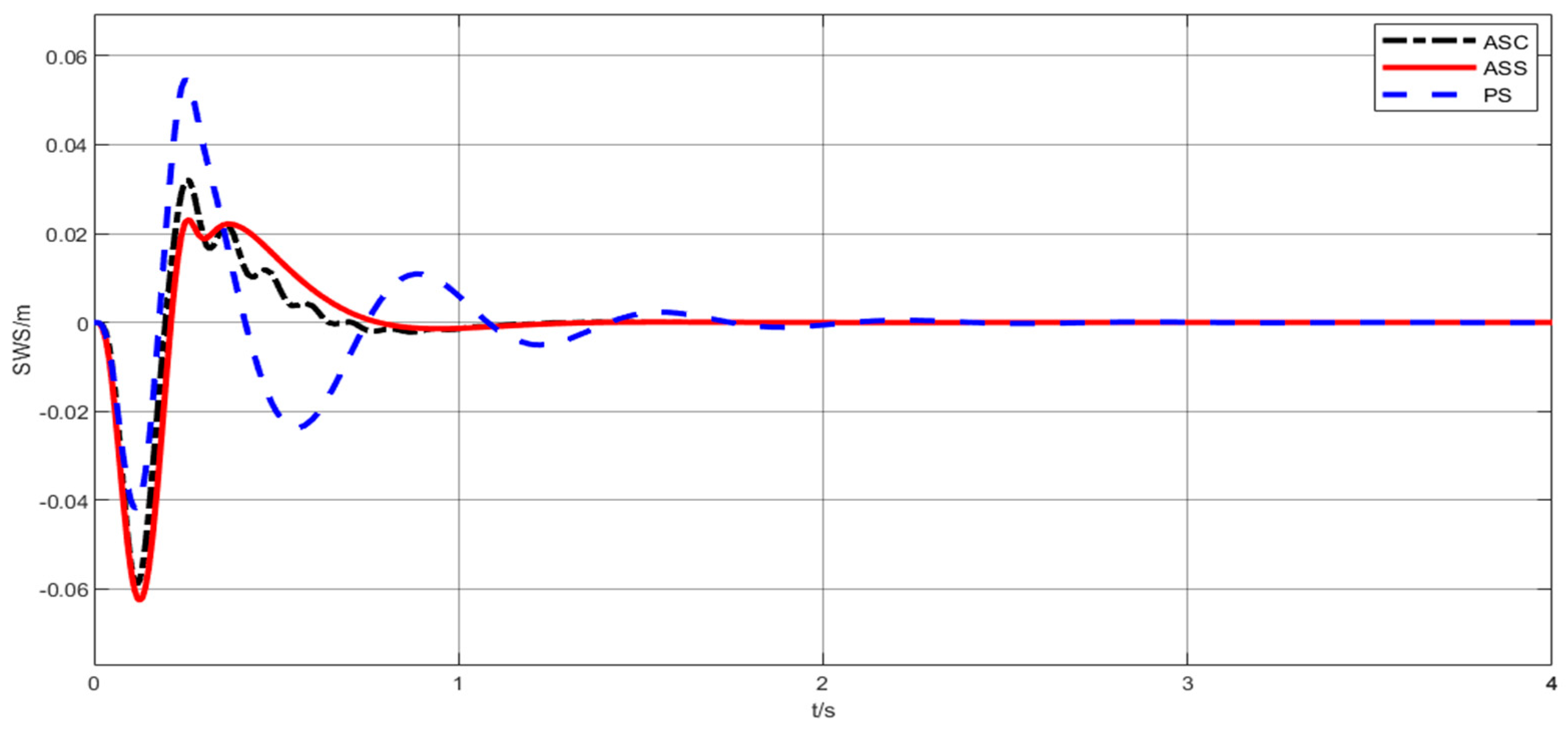
To further evaluate the effectiveness of the designed controller, three kinds of suspensions consisting of passive suspension (PS), active suspension with suspended IWM absorber (ASS), active suspension with centralized IWM (ASC) are implemented and compared, where the two active suspensions are designed with constrained H∞ controller. Three road responses, including BA, SWS, and DTD, for different suspensions under bump road excitation are depicted in Figure 10, Figure 11, Figure 12, Figure 13, Figure 14 and Figure 15; nominal system and perturbed system responses of the suspensions are shown in Figure 10, Figure 11, Figure 12, Figure 13, Figure 14 and Figure 15, in which the perturbed system takes into account 20% mass variation. As can be seen from these Figures, the BA and DTD responses of suspension controlled by the H∞ controller are much smaller than that with the passive suspension, even though mass variation with 20% exists. It is worth noting that controlled SWS of active suspension still operates in the constrained suspension deflections (less than ±0.08 m). Moreover, it is clear that the vehicle ASS achieves better passenger comfort and road holding ability compared with ASC and PS.
5. Conclusions
A constrained robust H∞ controller of active suspension system for IWMD-EV considering control constraint and parameter variation is proposed. Parameter uncertainties in the active suspension system model are analyzed, and control constraints of suspension performance for constrained robust H∞ controller design are also investigated. Simulations, including random and bump road excitations, are implemented to verify the effectiveness of the proposed controller. It is confirmed from the simulation results that the designed controller possesses improved ride comfort and road-holding ability performance in spite of control constraints and parameter variations. Moreover, this study also reveals that the potential of an active suspension system for IWMD-EV can be improved by developing robust control strategies. In the future, we will further research and compare various control techniques for other active suspension systems with different topology structures in IWMD-EV. Besides, we will explore and extend the applicability of the developed control method in other different areas, such as vehicle lateral dynamics and integrated vehicle handling and stability.
Author Contributions
Conceptualization, X.J., J.W., S.S., J.Y., Z.Y.; supervision, X.J.; conception and design, X.J., J.W., S.S.; collection and assembly of data, X.J., J.W., J.Y.; manuscript writing, X.J., J.W., Z.Y., S.L.; funding, X.J., S.L. All authors have read and agreed to the published version of the manuscript.
Funding
This work is supported by the National Science Foundation of China (51905329), State Key Laboratory of Mechanical Behavior and System Safety of Traffic Engineering Structure (KF2020-26).
Institutional Review Board Statement
Not applicable.
Informed Consent Statement
Not applicable.
Data Availability Statement
Data sharing not applicable.
Conflicts of Interest
The authors declare no conflict of interest.
References
- Jin, X.; Yu, Z.; Yin, G.; Wang, J. Improving vehicle handling stability based on combined AFS and DYC system via robust Takagi-Sugeno fuzzy control. IEEE Trans. Intell. Transp. Syst. 2017, 19, 2696–2707. [Google Scholar] [CrossRef]
- Goodarzi, A.; Esmailzadeh, E. Design of a VDC system for all-wheel independent drive vehicles. IEEE/ASME Trans. Mechatron. 2007, 12, 632–639. [Google Scholar] [CrossRef]
- Chen, Y.; Hedrick, J.K.; Guo, K. A novel direct yaw moment controller for in-wheel motor electric vehicles. Veh. Syst. Dyn. 2013, 51, 925–942. [Google Scholar] [CrossRef]
- Jin, X.; Yin, G.; Chen, J.; Chen, N. Robust guaranteed cost state-delayed control of yaw stability for four-wheel-independent-drive electric vehicles with active front steering system. Int. J. Veh. Design. 2015, 69, 304–323. [Google Scholar] [CrossRef]
- Zheng, B.; Anwar, S. Yaw stability control of a steer-by-wire equipped vehicle via active front wheel steering. Mechatronics 2009, 19, 799–804. [Google Scholar] [CrossRef]
- Nam, K.; Fujimoto, H.; Hori, Y. Advanced motion control of electric vehicles based on robust lateral tire force control via active front steering. IEEE/ASME Trans. Mechatron. 2012, 19, 289–299. [Google Scholar] [CrossRef]
- Hu, C.; Wang, R.; Yan, F.; Chen, N. Output constraint control on path following of four-wheel independently actuated autonomous ground vehicles. IEEE Trans. Veh. Technol. 2015, 65, 4033–4043. [Google Scholar] [CrossRef]
- Poussot-Vassal, C.; Sename, O.; Dugard, L.; Savaresi, S.M. Vehicle dynamic stability improvements through gain-scheduled steering and braking control. Veh. Syst. Dyn. 2011, 49, 1597–1621. [Google Scholar] [CrossRef] [Green Version]
- Yang, X.; Wang, Z.; Peng, W. Coordinated control of AFS and DYC for vehicle handling and stability based on optimal guaranteed cost theory. Veh. Syst. Dyn. 2009, 47, 57–79. [Google Scholar] [CrossRef]
- Ivanov, V.; Savitski, D.; Shyrokau, B. A survey of traction control and antilock braking systems of full electric vehicles with individually controlled electric motors. IEEE Trans. Veh. Technol. 2014, 64, 3878–3896. [Google Scholar] [CrossRef]
- Han, K.; Lee, B.; Choi, S.B. Development of an antilock brake system for electric vehicles without wheel slip and road friction information. IEEE Trans. Veh. Technol. 2019, 68, 5506–5517. [Google Scholar] [CrossRef]
- Jin, X.; Yin, G.; Zeng, X.; Chen, J. Robust Gain-scheduled Output Feedback Yaw Stability Control for Four-Wheel-Independent-Drive Electric Vehicles with External Yaw-Moment. J. Frankl. Inst. 2018, 355, 9271–9297. [Google Scholar] [CrossRef]
- Luo, Y.; Tan, D. Study on the dynamics of the in-wheel motor system. IEEE Trans. Veh. Technol. 2012, 61, 3510–3518. [Google Scholar]
- Bridgestone, C. Bridgestone Dynamic-Damping In-Wheel Motor Drive System. 2017. Available online: http://enginuitysystems.com/files/In-Wheel_Motor.pdf (accessed on 25 December 2017).
- Kulkarni, A.; Ranjha, S.A.; Kapoor, A. A quarter-car suspension model for dynamic evaluations of an in-wheel electric vehicle. Proc. Inst. Mech. Eng. Part D 2018, 232, 1139–1148. [Google Scholar] [CrossRef]
- Yang, F.; Zhao, L.; Yu, Y.; Zhou, C. Analytical description of ride comfort and optimal damping of cushion-suspension for wheel-drive electric vehicles. Int. J. Autom. Technol. 2017, 18, 1121–1129. [Google Scholar] [CrossRef]
- Wang, W.; Niu, M.; Song, Y. Integrated Vibration Control of In-Wheel Motor-Suspensions Coupling System via Dynamics Parameter Optimization. Shock. Vib. 2019, 2019, 3702919. [Google Scholar] [CrossRef] [Green Version]
- Yin, G.; Chen, N.; Li, P. Improving Handling Stability Performance of Four-Wheel Steering Vehicle via mu-Synthesis Robust Control. IEEE Trans. Veh. Technol. 2007, 56, 2432–2439. [Google Scholar] [CrossRef]
- Karimi, H.R.; Duffie, N.A.; Dashkovskiy, S. Local capacity H∞ control for production networks of autonomous work systems with time-varying delays. IEEE Trans. Autom. Sci. Eng. 2009, 7, 849–857. [Google Scholar] [CrossRef]
- Shi, Y.; Yu, B. Output feedback stabilization of networked control systems with random delays modeled by Markov chains. IEEE Trans. Autom. Control. 2009, 54, 1668–1674. [Google Scholar]
- Qiu, J.; Ding, S.X.; Gao, H.; Yin, S. Fuzzy-Model-Based Reliable Static Output Feedback H∞ Control of Nonlinear Hyperbolic PDE Systems. IEEE Trans. Fuzzy Syst. 2016, 24, 388–400. [Google Scholar] [CrossRef]
- Kwon, B.S.; Kang, D.; Yi, K. Fault-tolerant control with state and disturbance observers for vehicle active suspension systems. Proc. Inst. Mech. Eng. D J. Autom. Eng. 2020, 234, 1912–1929. [Google Scholar] [CrossRef]
- Du, H.; Zhang, N. Designing H∞/GH2 static-output feedback controller for vehicle suspensions using linear matrix inequalities and genetic algorithms. Veh. Syst. Dyn. 2008, 46, 385–412. [Google Scholar] [CrossRef]
- Li, P.; Lam, J.; Cheung, K.C. Multi-objective control for active vehicle suspension with wheelbase preview. J. Sound Vib. 2014, 333, 5269–5282. [Google Scholar] [CrossRef]
- Li, H.; Liu, H.; Gao, H.; Shi, P. Reliable fuzzy control for active suspension systems with actuator delay and Fault. IEEE Trans. Fuzzy Syst. 2011, 20, 342–357. [Google Scholar] [CrossRef] [Green Version]
- Jin, X.; Yin, G.; Bian, C.; Chen, J.; Li, P.; Chen, N. Gain-scheduled vehicle handling stability control via integration of active front steering and suspension systems. ASME Trans. J. Dyn. Syst. Meas. Control. 2016, 138, 014501. [Google Scholar] [CrossRef]
- Morato, M.M.; Normey-Rico, J.E.; Sename, O. Sub-optimal recursively feasible Linear Parameter-Varying predictive algorithm for semi-active suspension control. IET Control Theory Appl. 2020, 14, 2764–2775. [Google Scholar] [CrossRef]
- Na, J.; Huang, Y.; Wu, X.; Su, S.; Li, G. Adaptive finite-time fuzzy control of nonlinear active suspension systems with input delay. IEEE Trans. Cybern. 2020, 50, 2639–2650. [Google Scholar] [CrossRef] [Green Version]
- Liu, Y.; Chen, H. Adaptive sliding mode control for uncertain active suspension systems with prescribed performance. IEEE Trans. Syst. Man Cybern. Syst. 2020, in press. [Google Scholar] [CrossRef]
- Dinh, H.T.; Trinh, T.D.; Tran, V.N. Saturated RISE feedback control for uncertain nonlinear Macpherson active suspension system to improve ride comfort. ASME Trans. J. Dyn. Syst. Meas. Control. 2020, 143, 011004. [Google Scholar] [CrossRef]
- Jin, X.; Yang, J.; Li, Y.; Zhu, B.; Wang, J.; Yin, G. Online estimation of inertial parameter for lightweight electric vehicle using dual unscented Kalman filter approach. IET Intell. Transp. Syst. 2020, 14, 412–422. [Google Scholar] [CrossRef]
- Jin, X.; Yin, G.; Chen, N. Advanced Estimation Techniques for Vehicle System Dynamic State: A Survey. Sensors 2019, 19, 4289. [Google Scholar] [CrossRef] [PubMed] [Green Version]
- Boyd, S.; Ghaoui, L.E.; Feron, E.; Balakishnan, V. Linear Matrix Inequalities in System and Control Theory; SIAM: Philadelphia, PA, USA, 1994; pp. 100–136. [Google Scholar]
Figure 1.
(a) Application model of an electric vehicle (EV) active suspension. (b) Quarter-car active suspension model.
Figure 1.
(a) Application model of an electric vehicle (EV) active suspension. (b) Quarter-car active suspension model.

Figure 2.
Schematic diagram of linear fractional transformation (LFT) structure.

Figure 3.
Schematic diagram of controller structure.

Figure 4.
The frequency response of body acceleration of the closed-loop system.

Figure 5.
The frequency response of suspension working space of the closed-loop system.

Figure 6.
The frequency response of dynamic tire displacement of the closed-loop system.

Figure 7.
Random road body acceleration responses of passive and active suspensions.

Figure 8.
Random road suspension working space responses of passive and active suspensions.

Figure 9.
Random road dynamic tire displacement responses of passive and active suspensions.

Figure 10.
Bump body acceleration responses of different suspensions.

Figure 11.
Bump suspension working space responses of different suspensions.

Figure 12.
Bump dynamic tire displacement responses of different suspensions.

Figure 13.
Bump body acceleration responses of different suspensions with 20% mass variation.

Figure 14.
Bump suspension working space responses of different suspensions with 20% mass variation.
Figure 14.
Bump suspension working space responses of different suspensions with 20% mass variation.

Figure 15.
Bump dynamic tire displacement responses of different suspensions with 20% mass variation.
Figure 15.
Bump dynamic tire displacement responses of different suspensions with 20% mass variation.


Table 1.
The parameters for the active suspension system.
| Parameter | Value | Parameter | Value |
|---|---|---|---|
| ms | 270 kg | mt | 40 kg |
| Ks | 22,000 N/m | mh | 30 kg |
| Kt | 220,000 N/m | Kh | 15,000 N/m |
| Cs | 200 Ns/m | dms | 0.2 |
Publisher’s Note: MDPI stays neutral with regard to jurisdictional claims in published maps and institutional affiliations. |
© 2021 by the authors. Licensee MDPI, Basel, Switzerland. This article is an open access article distributed under the terms and conditions of the Creative Commons Attribution (CC BY) license (http://creativecommons.org/licenses/by/4.0/).
Share and Cite
MDPI and ACS Style
Jin, X.; Wang, J.; Sun, S.; Li, S.; Yang, J.; Yan, Z. Design of Constrained Robust Controller for Active Suspension of In-Wheel-Drive Electric Vehicles. Mathematics 2021, 9, 249. https://doi.org/10.3390/math9030249
AMA Style
Jin X, Wang J, Sun S, Li S, Yang J, Yan Z. Design of Constrained Robust Controller for Active Suspension of In-Wheel-Drive Electric Vehicles. Mathematics. 2021; 9(3):249. https://doi.org/10.3390/math9030249
Chicago/Turabian StyleJin, Xianjian, Jiadong Wang, Shaoze Sun, Shaohua Li, Junpeng Yang, and Zeyuan Yan. 2021. "Design of Constrained Robust Controller for Active Suspension of In-Wheel-Drive Electric Vehicles" Mathematics 9, no. 3: 249. https://doi.org/10.3390/math9030249
Note that from the first issue of 2016, this journal uses article numbers instead of page numbers. See further details here.