
Approximation of the Constant in a Markov-Type Inequality on a Simplex Using Meta-Heuristics


1
Department of Topology and Algebra, Rzeszow University of Technology, Powstancow Warszawy 12, 35-959 Rzeszow, Poland
2
Department of Computer and Control Engineering, Rzeszow University of Technology, Wincentego Pola 2, 35-959 Rzeszow, Poland
*
Author to whom correspondence should be addressed.
Mathematics 2021, 9(3), 264; https://doi.org/10.3390/math9030264
Submission received: 20 December 2020
/
Revised: 21 January 2021
/
Accepted: 26 January 2021
/
Published: 29 January 2021
(This article belongs to the Special Issue Nonlinear Problems and Applications of Fixed Point Theory)
Abstract
:Markov-type inequalities are often used in numerical solutions of differential equations, and their constants improve error bounds. In this paper, the upper approximation of the constant in a Markov-type inequality on a simplex is considered. To determine the constant, the minimal polynomial and pluripotential theories were employed. They include a complex equilibrium measure that solves the extreme problem by minimizing the energy integral. Consequently, examples of polynomials of the second degree are introduced. Then, a challenging bilevel optimization problem that uses the polynomials for the approximation was formulated. Finally, three popular meta-heuristics were applied to the problem, and their results were investigated.
1. Introduction
Markov-type polynomial inequalities (or inverse inequalities) [1,2,3,4,5,6], similarly to Bernstein-type inequalities [1,5,6,7,8,9], are often found in many areas of applied mathematics, including popular numerical solutions of differential equations. Proper estimates of optimal constants in both types of inequalities can help to improve the bounds of numerical errors. They are often used in the error analysis of variational techniques, including the finite element method or the discontinuous Galerkin method used for solving partial differential equations (PDEs) [10]. Moreover, Markov’s inequality can be found in constructions of polynomial meshes, as it is a representative sampling method, and is used as a tool for studying the uniform convergence of discrete least-squares polynomial approximations or for spectral methods for the solutions of PDEs [11,12,13]. Generally, finding exact values of optimal constants in a given compact set E in is considered particularly challenging. In this paper, an approach to determining the upper estimation of the constant in a Markov-type inequality on a simplex is proposed. The method aims to provide a greater value than that estimated by L. Bialas-Ciez and P. Goetgheluck [4].
For an arbitrary algebraic polynomial P of N variables and degree not greater than n, Markov’s inequality is expressed as
where , E is a convex compact subset of (with non-void interior), and The exponent 2 in (1) is optimal for a convex compact set E (with non-void interior) [2,4].
In 1974, D. Wilhelmsen [14] got an upper estimate for the constant in Markov’s inequality (1), where is the width of E. The width of is defined as [4], where G is the set of all possible couples of parallel planes and such that E lies between and Furthermore, for any convex compact set , the author proposed the hypothesis that M. Baran [3,7] and Y. Sarantopoulos [15] independently proved that Wilhelmsen’s conjecture is true for centrally symmetric convex compact sets. In turn, L. Bialas-Ciez and P. Goetgheluck [4] showed that the hypothesis is false in the simplex case and proved that the constant
The best constant in Markov’s inequality (1) for a convex set was also studied by D. Nadzhmiddinow and Y. N. Subbotin [6] and by A. Kroó and S. Révész [16]. It is worth mentioning that for any triangles in , A. Kroó and S. Révész [16] generalized the result for a simplex given in [4], considering an admissible upper bound for , and received an upper estimate value of constant C in (1): where with being a triangle with the sides and the angles , respectively, such that and
In the recent literature, many works have considered Markov inequalities. For example, S. Ozisik et al. [10] determined the constants in multivariate Markov inequalities on an interval, a triangle, and a tetrahedron with the -norm. They derived explicit expressions for the constants on all above-mentioned simplexes using orthonormal polynomials. It is worth noticing that exact values of the constants are the key for the correct derivation of both a priori and a posteriori error estimates in adaptive computations. F. Piazzon and M. Vianello [11] used the approximation theory notions of a polynomial mesh and the Dubiner distance in a compact set to determine error estimates for the total degree of polynomial optimization on Chebyshev grids of the hypercube. Additionally, F. Piazzon and M. Vianello [12] constructed norming meshes for polynomial optimization by using a classical Markov inequality on the general convex body in . A. Sommariva and M. Vianello [13] used discrete trigonometric norming inequalities on subintervals of the period. They constructed norming meshes with optimal cardinality growth for algebraic polynomials on the sections of a sphere, a ball, and a torus. Moreover, A. Kroó [17] studied the so-called optimal polynomial meshes and O. Davydov [18] presented error bounds for the approximation in the space of multivariate piecewise polynomials admitting stable local bases. In particular, the bounds apply to all spaces of smooth finite elements, and they are used in the finite element method for general fully nonlinear elliptic differential equations of the second order. L. Angermann and Ch. Heneke [19] proved error estimates for the Lagrange interpolation and for discrete -projection, which were optimal on the elements and almost optimal on the element edges. In another study, M. Bun and J. Thaler [5] reproved several Markov-type inequalities from approximation theory by constructing explicit dual solutions to natural linear programs. Overall, these inequalities are a basis for proofs of many approximated solutions that can be found in the literature.
In this paper, an approach to determining an approximation of the constant in Markov’s inequality using introduced minimal polynomials is proposed. Then, the polynomials are used in the formulated bilevel optimization problem. Since many optimization techniques could be employed to find the constant, three popular meta-heuristics are applied and their results are investigated.
The rest of this paper is structured as follows. In Section 2, minimal polynomials are introduced. Then, in Section 3, their application in the approximation of the constant in a Markov-type inequality is considered. In Section 4, in turn, the approximation is defined as an optimization problem and the problem is solved using three meta-heuristics. Finally, in Section 5, the study is summarized and directions for future work are indicated.
2. Minimal Polynomials
The monic polynomial is defined as: for each , and with [20,21,22] (the coefficient of its leading monomial is equal 1), where is its length and ≺ indicates the graded lexicographic order, defined as: If , then , while if when , the first (starting from the left) non-zero coefficient of is positive [21,22]. Polynomial of the smallest deviation from zero on E with respect to the supremum norm is called the minimal polynomial (Chebyshev polynomial) for E [22,23,24,25].
Let E be a compact set in a complex plane that contains at least points. Based on the classical theorem of Tonelli [26], among the monic polynomials of degree , there exists only one polynomial that minimizes the supremum norm on E. The is called the Chebyshev polynomial of order It is defined as , where the infimum is taken with respect to In other words, is the polynomial of best approximation to on This polynomial is called the minimal (monic) polynomial of degree
The complex equilibrium measure for a standard simplex in is calculated for , which is a simplex in [8]. Then, the plurisubharmonic extremal function on E, is used to calculate the (complex) equilibrium measure , where is the usual volume of the closed-unit Euclidean ball in .
3. Estimation of the Constant in a Markov-Type Inequality
Let be a simplex in Consequently,
The normalized equilibrium measure , as a subset of , is a two-dimensional Lebesgue measure with the weight For continuous functions on , the scalar product is defined as
Then, a polynomial is defined. It is the minimal polynomial for the simplex, and for some real numbers , , , , , and Thus,
where for are symbols given in Table 1.
We want the polynomial P to be orthogonal to Q so that Substituting the values given in Table 1 into the expression above, is obtained. Finally,
Here, a counterexample to the Wilhelmsen hypothesis can be formulated, which is different from that discussed by L. Bialas-Ciez and P. Goetgheluck [4], to support the claim that the approach leads to a better approximation. Counterexample: Consider the following polynomial , where Putting , is obtained. It is easy to calculate that is reached for point , and its value is Similarly, Hence, this simple and far from optimal approximation value is greater than those of L. Bialas-Ciez and P. Goetgheluck [4]:
4. Optimization Problem in a Markov-Type Inequality
The estimation of the constant C in Markov’s inequality can be improved by considering a minimal polynomial and an equilibrium measure. The exemplary calculations of minimal polynomials and their corresponding Markov inequalities on the simplex are shown in Table 2. In the first example of the polynomial, the obtained constant is equal to the value reported by L. Bialas-Ciez and P. Goetgheluck [4]. In the remaining two polynomials, the constants are improved. However, a slight change in the coefficients decreases the constant, as is shown in the fourth example. Therefore, in this paper, the polynomial is proposed as a result of a nontrivial optimization problem in which an improvement of the estimate of the constant C is considered.
In this paper, the constant in Markov’s inequality on the simplex for the proposed minimal polynomials is estimated. Assuming that
where P is one of the following minimal polynomials:
and , in order to determine the greatest value of the function an optimization problem is formulated.
R. M. Aron and M. Klimek [27] gave explicit formulas for supremum norms: and where
The vectors and are regarded as decision variables in the optimization problem. Consequently, and denote the vectors that maximize the . Considering the relationship between and or and only the coefficients that maximize their corresponding and need to be found, i.e., they are then applied to the remaining polynomials. For polynomials and The calculation of Equation (2) requires finding the extrema of the polynomial P inside the simplex limited by values . Therefore, the following bilevel optimization problem is solved. Here, one optimization task is nested within the other, i.e., the decision variables of the upper problem are the parameters in the lower one, and the lower problem is a constraint to the upper problem, limiting the feasible u values to those that are lower-level optimal [28].
The problem is given by
where denotes the arguments of the function that maximize its value.
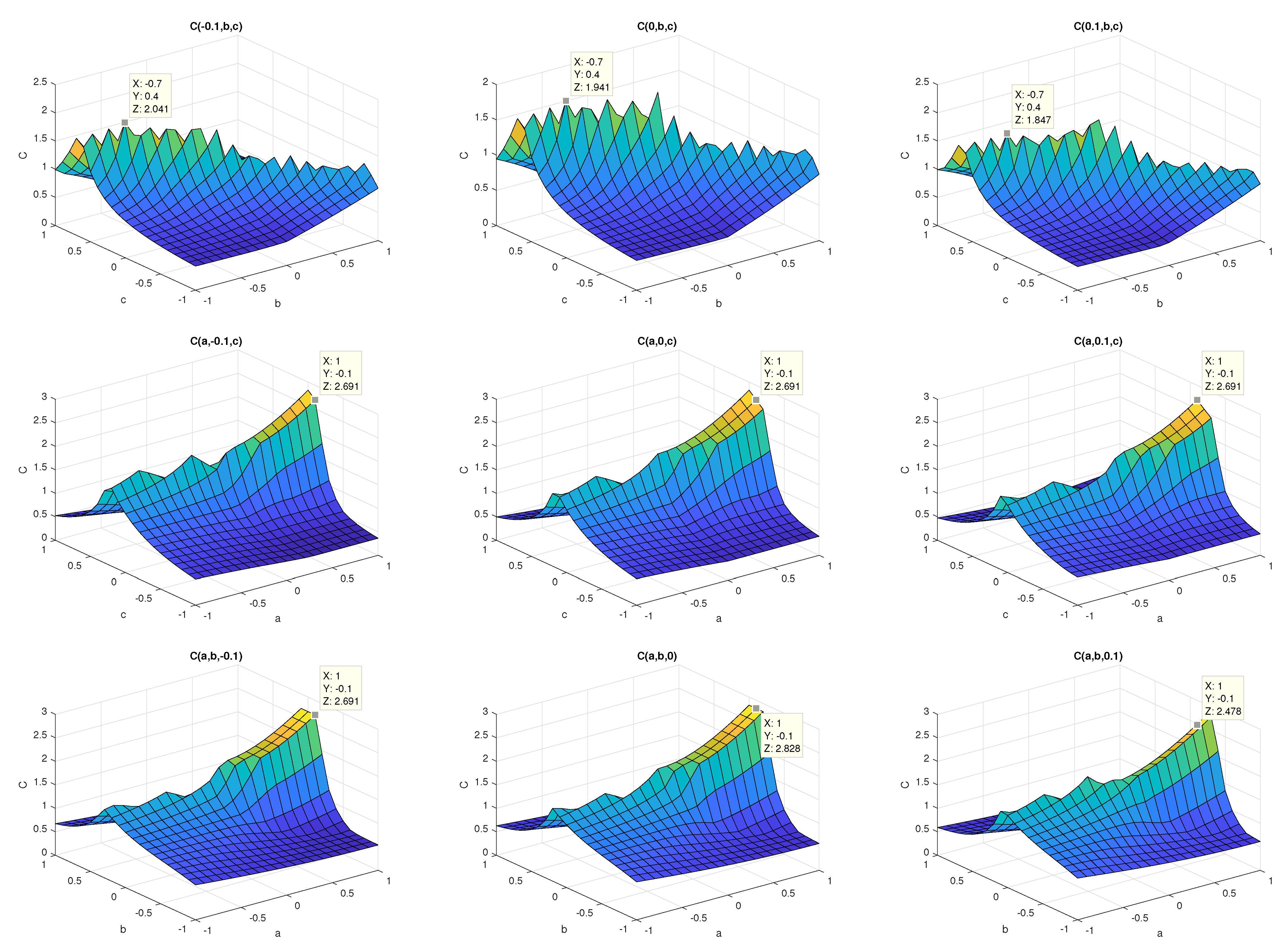
Finally, the values of and are found as the solutions to the optimization problem. In order to determine the greatest value of C, the nonlinearity of the considered objective function, as well as the existence of multiple local optima, must be taken into account. Here, different values of u can lead to the same value of C, or close values of u can result in a large difference between the corresponding values of This can be seen in Figure 1, in which only a small part of the search space is visualized. For the visualization, C is calculated, keeping one coefficient constant and selecting the remaining one from the range with the step . The coefficients are selected from the set The difference between the values of the constant is purposely small to show the changes of values of Each subplot in Figure 1 contains a marker to additionally highlight such changes.
To solve the defined optimization problem, a suitable method should be determined. Therefore, in this paper, a hybrid approach is proposed. It is justified by the need to find the extrema of the polynomial P inside the simplex for the computation of C. Such extrema are found using the Interior Point Algorithm (IPT) [29,30], i.e., is found for an examined u from the upper level. The upper-level optimization is more difficult. Since the considered problem has not been formulated and solved in the literature, it cannot be determined in advance which method should be used to determine the solution. Therefore, taking into account possible time-consuming computations, three popular meta-heuristics are used and compared: the Particle Swarm Optimization method (PSO) [31,32,33], Genetic Algorithm (GA) [34,35], and Simulated Annealing technique (SA) [36,37]. The application of population-based algorithms for solving different bilevel problems is popular (e.g., [28]).
The PSO is a global evolutionary method based on swarm intelligence. It finds the optimal solution by exploring the search space using a set of particles. Each particle represents a candidate solution to the problem. The PSO mimics the movement of a bird flock or a fish school; hence, the dynamics of the set of particles in the solution space are iteratively governed by the following equations [31]:
where and are the position and the velocity of the i-th particle at time ; is the best position of the i-th particle, while is the best position of the swarm at n. w is the inertia weight, and and are coefficients constraining the parts of the equation that simulate cognitive and social factors of the swarm [31,32,33]); and are random numbers drawn from the range . The termination criterion of the algorithm is the number of iterations N or the violation of the minimal acceptable difference in the objective function C between consecutive iterations. Both criteria are commonly used in most heuristic optimization algorithms. Finally, the PSO returns .
The GA uses a population of individuals (called chromosomes), representing candidate solutions [34,35]. In the GA, at each generation (iteration), a population of individuals is assessed to select the best solutions, which are then used to create the population in the next generation. The assessment is based on the values of the objective function, while new individuals are obtained using crossover and mutation operators. The crossover combines the information carried by two selected parents in one solution by mixing values of their vector representations. The mutation, in turn, introduces random changes to the individual. After the predefined number of generations, the algorithm returns the best individual .
The simulated annealing, unlike the population-based PSO and GA, uses much fewer resources and requires fewer objective function computations, since it processes only one solution at each iteration [36,37]. The SA mimics the process of heating a metal and slowly lowering its temperature. The algorithm starts from a random solution, which is iteratively modified. At each iteration, reflecting a temperature drop, the algorithm modifies the current solution and compares the values of the objective function before and after the modification. If a new solution is better or the difference between their values is within a predefined range, the modification is accepted. The acceptance of a slightly worse solution helps the method to escape local minima [36,37].
All of these methods are commonly used for solving nonlinear optimization problems with local optima. However, their suitability for a given problem is mostly determined experimentally. In this paper, they are used to determine . However, in order to calculate C for any u, the lower-level optimum must be solved each time. In this paper, it is obtained using the IPT algorithm [29,30]. Finally, the considered problem is solved using the hybrid approach [28]. In the IPT algorithm, an optimization problem is defined as
where is objective function to be minimized and h and g are equality and inequality constraints, respectively. The solved approximate problem is defined as
where are slack variables and is a barrier parameter. As converges to zero, the sequence of approximate solutions converges to the minimum of f [29,30].
In the numerical experiments, the solution processed by heuristic algorithms was represented by a five-dimensional vector of floating-point values, since , and the IPT used a two-dimensional vector . To ensure a fair comparison of meta-heuristics, each technique was run 50 times, and a maximum of 25,000 objective function calls were performed in each run. The number of function calls was achieved by selecting a large-enough population size, aiming at the best performance of the PSO and GA. The implementations of the algorithms that can be found in the Matlab Optimization Toolbox are used. Algorithms were run with their default parameters: the PSO (w = [01, 1.1], , ), the GA (EliteCount = 0.05 of the population size, CrossoverFraction = 0.8, the scattered crossover, Gaussian mutation, and stochastic uniform selection), and the SA (InitialTemperature = 100, temperature is equal to InitialTemperature * 0.95). Note that the values in u were not bounded (i.e., ), and the GA and PSO, unlike the SA, did not require the specification of the starting point of the optimization, as the initial populations of the solutions were selected randomly. For this reason, the SA started from . As demonstrated in Table 3, the PSO was able to determine the best C for each polynomial. The algorithms explored the solution space in different ways, obtaining different results.
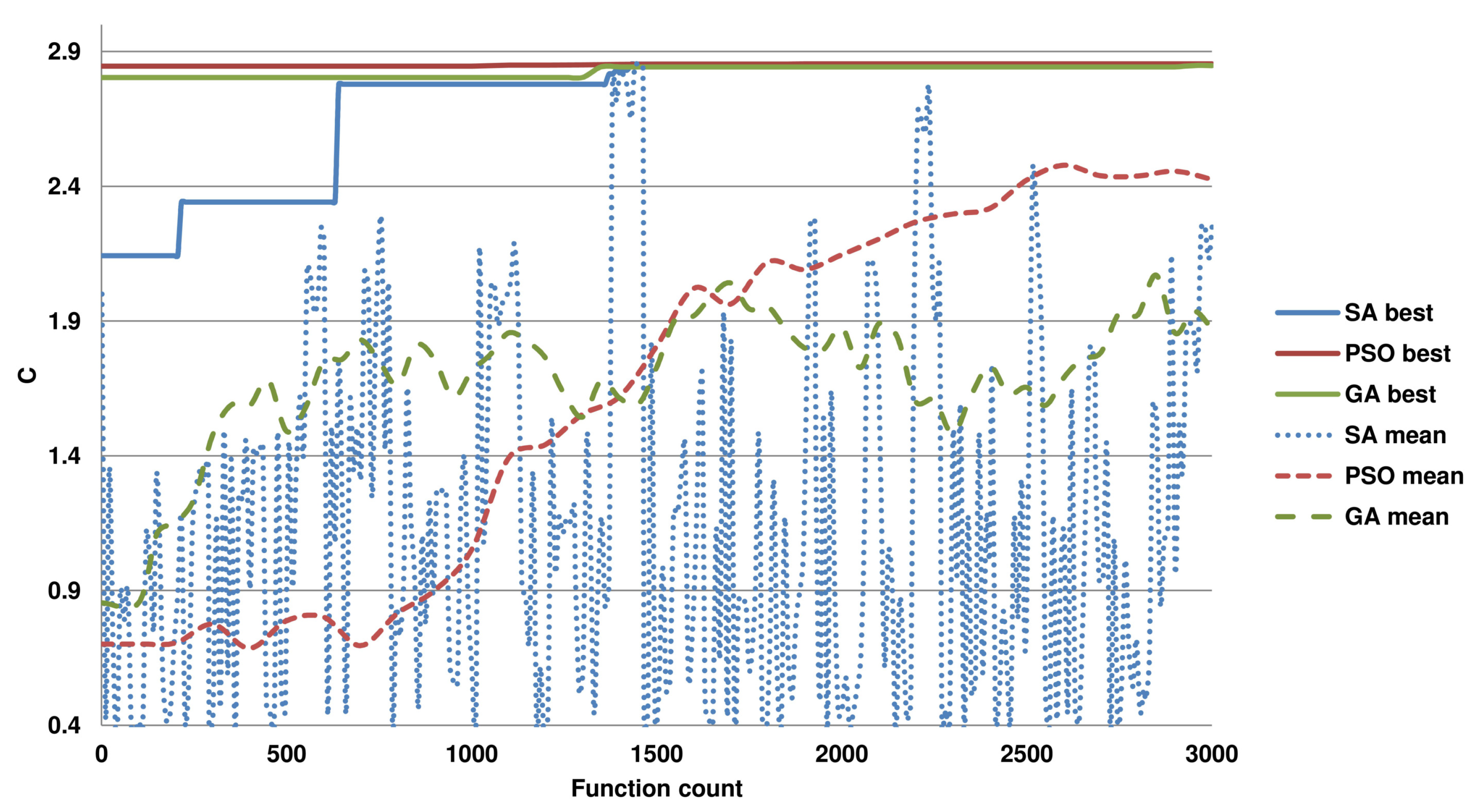
To further show the difficulty of the optimization task for the used algorithms, Figure 2 presents the convergence of the algorithms towards the optimum. Here, the progress of the set of solutions at each calculation of the objective function is reported. As presented, the approaches with the PSO and GA quickly converge, and most of the time is spent on the exploration of the solution space near the optimum. The SA, unlike the population-based methods, processes one solution at each iteration, which influences its convergence rate. The results reveal that the PSO is better suited to the problem than the GA, since it can determine a better C (see Table 3), and it finds it with fewer function calls. Interestingly, the set of solutions in the first function call is more diverse for the PSO, which may contribute to its superior performance, as in the remaining computation time, it is more focused on escaping the local optima. Similarly, it can be seen that the solutions emerging in the run of the SA exhibit large variability. Note that the number of runs (50) and the maximal number of function calls in these experiments (25,000) are purposely greater than could be concluded from the convergence plots to give the methods enough resources to find better solutions. However, the methods often terminate the computations if the change in the best function value is too small.
This experiment indicates that the proposed approach with the PSO can provide the best C. Therefore, in the second experiment, the parameters of this algorithm were set to conduct an even better search of the solution space. By increasing the number of particles and generations, the maximal number of function calls was set to 25 million, and the method was run 100 times. Note that the estimated time to finish one run of the PSO with 25 million function calls in Matlab on the i7-6700 K 4 GHz with 64 GB RAM CPU is 335 h. The calculations were run in a parallel manner, and the methods were allowed to terminate the optimization if a function value change was small. They are presented in Table 4. The second experiment improved the already obtained values for (or ) and (or ) at the fifth and eighth decimal places, respectively (see Table 3). The run in which the best was obtained required 720 thousand function calls, and was found in a run after the objective function was calculated 1570 thousand times.
5. Conclusions
In this paper, it was demonstrated that the best constant C in Markov’s inequality for the minimal polynomials on the simplex can be determined as a solution to a nested optimization problem. First, the examples of the polynomials that allow estimation of the constant were proposed. Then, the optimization problem was defined and its solution was investigated. Since it could not be determined in advance which heuristic optimization algorithm should be used, three popular meta-heuristics were adopted and compared. Finally, the optimal value of the constant was obtained with a hybrid of the ITP and PSO.
Future work will focus on the application of the polynomials of the higher degrees to the considered problem. In addition, the usage of the introduced bilevel optimization problem as an evaluation tool for the comparison of the performance of meta-heuristics seems to be a promising future direction.
Author Contributions
Conceptualization, G.S. and M.O.; methodology, G.S. and M.O.; software, M.O.; validation, G.S. and M.O.; formal analysis, G.S.; investigation, G.S. and M.O.; writing—original draft preparation, G.S. and M.O.; writing—revised draft preparation, G.S. and M.O. All authors have read and agreed to the published version of the manuscript.
Funding
This research received no external funding.
Conflicts of Interest
The authors declare no conflict of interest.
References
- Baran, M.; Bialas-Ciez, L. On the behaviour of constants in some polynomial inequalities. Ann. Pol. Math. 2019, 123, 43–60. [Google Scholar] [CrossRef]
- Baran, M.; Bialas-Ciez, L.; Milowka, B. On the best exponent in Markov’s inequality. Potential Anal. 2013, 38, 635–651. [Google Scholar] [CrossRef] [Green Version]
- Baran, M. Markov inequality on sets with polynomial parametrization. Ann. Polon. Math. 1994, 60, 69–79. [Google Scholar] [CrossRef]
- Bialas-Ciez, L.; Goetgheluck, P. Constants in Markov’s inequality on convex sets. East J. Approx. 1995, 1, 379–389. [Google Scholar]
- Bun, M.; Thaler, J. Dual lower bounds for approximate degree and Markov-Bernstein inequalities. Inf. Comput. 2015, 243, 2–25. [Google Scholar] [CrossRef]
- Nadzhmiddinov, D.; Subbotin, Y.N. Markov Inequalities for Polynomials on Triangles. Math. Notes Acad. Sci. USSR 1989, 46, 627–631. [Google Scholar] [CrossRef]
- Baran, M. Bernstein type theorems for compact sets in revisited. J. Approx. Theory 1994, 79, 190–198. [Google Scholar] [CrossRef] [Green Version]
- Baran, M. Complex equilibrium measure and Bernstein type theorems for compact sets in . Proc. Amer. Math. Soc. 1995, 123, 485–494. [Google Scholar]
- Sofonea, F.; Tincu, I. On an Inequality for Legendre Polynomials. Mathematics 2020, 8, 2044. [Google Scholar] [CrossRef]
- Ozisik, S.; Riverce, B.; Warburon, T. On the Constants in Inverse Inequalities in L2. Technical Report. 2010. Available online: https://hdl.handle.net/1911/102161 (accessed on 5 December 2020).
- Piazzon, F.; Vianello, M. A note on total degree polynomial optimization by Chebyshev grids. Optim. Lett. 2018, 12, 63–71. [Google Scholar]
- Piazzon, F.; Vianello, M. Markov inequalities, Dubiner distance, norming meshes and polynomial optimization on convex bodies. Optim. Lett. 2019, 13, 1325–1343. [Google Scholar] [CrossRef]
- Sommariva, A.; Vianello, M. Discrete norming inequalities on sections of sphere, ball and torus. arXiv 2018, arXiv:1802.01711. [Google Scholar]
- Wilhelmsen, D.R. A Markov inequality in several dimensions. J. Approx. Theory 1974, 11, 216–220. [Google Scholar] [CrossRef] [Green Version]
- Sarantopoulos, Y. Bounds on the derivatives of polynomials on Banach spaces. Math. Proc. Camb. Philos. Soc. 1991, 110, 307–312. [Google Scholar] [CrossRef]
- Kroó, A. Révész, S. On Bernstein and Markov-type inequalities for multivariate polynomials on convex bodies. J. Approx. Theory 1999, 99, 134–152. [Google Scholar] [CrossRef] [Green Version]
- Kroó, A. On the existence of optimal meshes in every convex domain on the plane. J. Approx. Theory 2019, 238, 26–37. [Google Scholar] [CrossRef] [Green Version]
- Davydov, O. Smooth Finite Elements and Stable Splitting; Berichte “Reihe Mathe-matik” der Philipps-Universit at Marburg: Marburg, Germany, 2007. [Google Scholar]
- Angermann, L.; Heneke, C. Interpolation, Projection and Hierarchical Bases in Discontinuous Galerkin Methods. Numer. Math. Theory Methods Appl. 2015, 8, 425–450. [Google Scholar] [CrossRef] [Green Version]
- Baran, M.; Kowalska, A.; Ozorka, P. Optimal factors in Vladimir Markov’s inequality in L2 Norm. Sci. Tech. Innov. 2018, 2, 64–73. [Google Scholar]
- Bialas-Ciez, L.; Jedrzejowski, M. Transfinite Diameter of Bernstein Sets in . J. Inequal. Appl. 2002, 7, 393–404. [Google Scholar]
- Bloom, T.; Calvi, J.P. On multivariate minimal polynomials. Math. Proc. Camb. Phil. Soc. 2000, 129, 417–432. [Google Scholar] [CrossRef]
- Bialas-Ciez, L.; Calvi, J.P. Homogeneous minimal polynomials with prescribed interpolation conditions. Proc. Am. Math. Soc. 2016, 368, 8383–8402. [Google Scholar] [CrossRef]
- Newman, D.J.; Xu, Y. Tchebycheff polynomials on a triangular region. Constr. Approx 1993, 9, 543–546. [Google Scholar] [CrossRef]
- Peherstorfer, F. Minimal polynomials for compact sets of the complex plane. Constr. Approx 1996, 12, 481–488. [Google Scholar] [CrossRef]
- Davis, P.J. Approximation and Interpolation; Dover Publication: New York, NY, USA, 1975. [Google Scholar]
- Aron, R.M.; Klimek, M. Supremum norms for quadratic polynomials. Arch. Math. 2001, 76, 73–80. [Google Scholar] [CrossRef]
- Sinha, A.; Malo, P.; Deb, K. Evolutionary algorithm for bilevel optimization using approximations of the lower level optimal solution mapping. Eur. J. Oper. Res. 2017, 257, 395–411. [Google Scholar] [CrossRef]
- Byrd, R.H.; Gilbert, J.C.; Nocedal, J. A Trust Region Method Based on Interior Point Techniques for Nonlinear Programming. Math. Prog. 2000, 89, 149–185. [Google Scholar] [CrossRef] [Green Version]
- Byrd, R.H.; Hribar, M.E.; Nocedal, J. An Interior Point Algorithm for Large-Scale Nonlinear Programming. SIAM J. Optim. 1999, 9, 877–900. [Google Scholar]
- Gao, Y.; Zhang, G.; Lu, J.; Wee, H.-M. Particle swarm optimization for bi-level pricing problems in supply chains. J. Glob. Optim. 2011, 51, 245–254. [Google Scholar] [CrossRef] [Green Version]
- Pedersen, M.E. Good Parameters for Particle Swarm Optimization; Hvass Laboratories: Luxembourg, 2010. [Google Scholar]
- Zhang, Y.; Wang, S.; Ji, G. A Comprehensive Survey on Particle Swarm Optimization Algorithm and Its Applications. Math. Probl. Eng. 2015, 2015, 38. [Google Scholar] [CrossRef] [Green Version]
- Goldberg, D.E. Genetic Algorithms in Search. In Optimization & Machine Learning; Addison-Wesley: Boston, MA, USA, 1989. [Google Scholar]
- Yang, J.; Zhang, M.; He, B.; Yang, C. Bi-level programming model and hybrid genetic algorithm for flow interception problem with customer choice. Comput. Math. Appl. 2009, 57, 1985–1994. [Google Scholar]
- Kirkpatrick, S.; Gelatt, C.D.; Vecchi, M.P. Optimization by Simulated Annealing. Science 1983, 220, 671–680. [Google Scholar] [PubMed]
- Sahin, K.H.; Ciric, A.R. A dual temperature simulated annealing approach for solving bilevel programming problems. Comput. Chem. Eng. 1998, 23, 11–25. [Google Scholar] [CrossRef]
Figure 1.
Influence of the coefficients u on the objective function . Three coefficients are selected: (first row), (second row), and (third row).
Figure 1.
Influence of the coefficients u on the objective function . Three coefficients are selected: (first row), (second row), and (third row).

Figure 2.
Convergence plots for the values of for sample runs of the hybrid approach with the Particle Swarm Optimization (PSO), Simulated Annealing (SA), and Genetic Algorithm (GA). The plots contain the best result at each function call and the mean value of for the processed solutions.
Figure 2.
Convergence plots for the values of for sample runs of the hybrid approach with the Particle Swarm Optimization (PSO), Simulated Annealing (SA), and Genetic Algorithm (GA). The plots contain the best result at each function call and the mean value of for the processed solutions.


Table 1.
Symbols and their values.
| SYMBOLS | ||||||||||
|---|---|---|---|---|---|---|---|---|---|---|
| VALUES |
Table 2.
Constants C in Markov inequalities on the simplex for exemplary polynomials.
| Example | Minimal Polynomial | |||
|---|---|---|---|---|
| 1 | 5/36 | /9 | C = 2.842534081 | |
| 2 | 99/784 | 10/168 | C = 2.850293143 | |
| 3 | 221/1760 | /40 | C = 2.851041419 | |
| 4 | 1/8 | C = 2.828427125 |
Table 3.
Optimization results obtained by the compared algorithms. The best values of C obtained in the first experiment are written in bold.
Table 3.
Optimization results obtained by the compared algorithms. The best values of C obtained in the first experiment are written in bold.
| Algorithm | ||
|---|---|---|
| GA | 2.861879141 | 2.852924202 |
| SA | 2.917638439 | 2.854084285 |
| PSO | 2.925401560 | 2.854206134 |
Table 4.
Values of C obtained in the second experiment and their corresponding coefficients.
| 2.925415050 | |
| −2765.096993 | |
| −1383.048545 | |
| −15148.04101 | |
| −10633.59420 | |
| 10846.85282 | |
| 2.854206170 | |
| 1.169292858 | |
| −0.121651344 | |
| −0.129695921 |
Publisher’s Note: MDPI stays neutral with regard to jurisdictional claims in published maps and institutional affiliations. |
© 2021 by the authors. Licensee MDPI, Basel, Switzerland. This article is an open access article distributed under the terms and conditions of the Creative Commons Attribution (CC BY) license (http://creativecommons.org/licenses/by/4.0/).
Share and Cite
MDPI and ACS Style
Sroka, G.; Oszust, M. Approximation of the Constant in a Markov-Type Inequality on a Simplex Using Meta-Heuristics. Mathematics 2021, 9, 264. https://doi.org/10.3390/math9030264
AMA Style
Sroka G, Oszust M. Approximation of the Constant in a Markov-Type Inequality on a Simplex Using Meta-Heuristics. Mathematics. 2021; 9(3):264. https://doi.org/10.3390/math9030264
Chicago/Turabian StyleSroka, Grzegorz, and Mariusz Oszust. 2021. "Approximation of the Constant in a Markov-Type Inequality on a Simplex Using Meta-Heuristics" Mathematics 9, no. 3: 264. https://doi.org/10.3390/math9030264
Note that from the first issue of 2016, this journal uses article numbers instead of page numbers. See further details here.