On a Discrete SEIR Epidemic Model with Exposed Infectivity, Feedback Vaccination and Partial Delayed Re-Susceptibility

Abstract

A new discrete Susceptible-Exposed-Infectious-Recovered (SEIR) epidemic model is proposed, and its properties of non-negativity and (both local and global) asymptotic stability of the solution sequence vector on the first orthant of the state-space are discussed. The calculation of the disease-free and the endemic equilibrium points is also performed. The model has the following main characteristics: (a) the exposed subpopulation is infective, as it is the infectious one, but their respective transmission rates may be distinct; (b) a feedback vaccination control law on the Susceptible is incorporated; and (c) the model is subject to delayed partial re-susceptibility in the sense that a partial immunity loss in the recovered individuals happens after a certain delay. In this way, a portion of formerly recovered individuals along a range of previous samples is incorporated again to the susceptible subpopulation. The rate of loss of partial immunity of the considered range of previous samples may be, in general, distinct for the various samples. It is found that the endemic equilibrium point is not reachable in the transmission rate range of values, which makes the disease-free one to be globally asymptotically stable. The critical transmission rate which confers to only one of the equilibrium points the property of being asymptotically stable (respectively below or beyond its value) is linked to the unity basic reproduction number and makes both equilibrium points to be coincident. In parallel, the endemic equilibrium point is reachable and globally asymptotically stable in the range for which the disease-free equilibrium point is unstable. It is also discussed the relevance of both the vaccination effort and the re-susceptibility level in the modification of the disease-free equilibrium point compared to its reached component values in their absence. The influences of the limit control gain and equilibrium re-susceptibility level in the reached endemic state are also explicitly made viewable for their interpretation from the endemic equilibrium components. Some simulation examples are tested and discussed by using disease parameterizations of COVID-19.

1. Introduction

Epidemic models have received much attention in the last decades. Many formulations used to describe them are based on either differential or difference equations leading to significant numbers of existing continuous-time and discrete-time epidemic models. For instance, the relevance of the basic reproduction number is discussed in [1] by obtaining related threshold theorems and applications to pertussis and measles descriptions. Feedback vaccination laws have been proposed by employing feedback control concepts and techniques as sliding-mode control or linear or impulsive feedback vaccination. See, for instance [2,3] and references therein. It has been described in the mentioned research how the various vaccination laws can affect the basic reproduction number, or the disease transmission rate, and then the stability of both the disease-free equilibrium point and the endemic one. The transient evolution of epidemic diseases is focused on in [4] to approximately predict the dates of maximum hospital occupancy of beds according to different epidemic models of continuous type, and the dates can be monitored to some extent under vaccination controls. The stability analysis and bifurcation control for a fractional order Susceptible-Infectious-Recovered (SIR) epidemic model with delay is focused on in [5]. The discretization of continuous-time epidemic models and the derivation of purely discrete epidemic models has also received much attention. See, for instance, [6,7,8,9,10,11,12] and references therein. It can be pointed out that, since the significant periods in a disease dynamics are relatively long, typically for instance on the orders of days or weeks, discrete-oriented epidemic models might be appropriate for the disease evolution efficient description and also to efficiently perform the computational studies to predict and eventually to control its transmission. A way of controlling the disease transmission is an appropriate programming of the vaccination campaigns. The above consideration is reinforced since the public vaccination policies are typically programmed for their management and administration to the population along coming periods of days or weeks, which are considered long periods for modelling discretization purposes and concerns that facilitate the decision implementations. Discretization techniques are in fact very useful in practical situations to accommodate the data acquisition from the disease evolution to its concrete use, interpretation and public decisions about the disease control when running through time mathematical epidemic models. In particular, an extended Susceptible-Exposed-Infectious-Recovered (SEIR) model which incorporates asymptomatic and dead infective subpopulations to the classical SEIR model has been discussed in [6] where the properties of stability of the equilibrium points and model positivity have been investigated in detail. Regular and impulsive feedback controls have been incorporated to the basic model. Such a model has been claimed to be of potential usefulness for Ebola evolution description. A multi-staged epidemic discrete model has been discussed in [7]. Although the exposed subpopulation is not included in such a model, it considers several coupled layers of the infectious subpopulation where the infection is transmitted from each layer to the adjacent ones. Discrete Susceptible-Infectious-Recovered-Susceptible (SIRS) models have also been studied in heterogeneous networks [8] with related bifurcation and stability studies. On the other hand, some epidemic models consider the vaccination actions as a generator of a new subpopulation, the vaccinated one, which is dynamically coupled to the remaining ones in the model rather than as a specific forcing control. See, for instance, [9]. In addition, discretized Susceptible-Infectious-Recovered (SIR)-type models, or Susceptible-Infectious-Susceptible (SIS)-type ones with stability formulations have been proposed in [10,11,12,13] and some of the references therein.

Over the last year, a lot of research has been developed concerning the recent COVID-19 pandemic. Since the authorities of the different countries supply very frequently disease registered data, typically day-to-day, such as infection and detection tests, hospital bed occupancies and, in particular, intensive unity care occupancies and mortality-related data, discrete epidemic models have been seen to be appropriate in the related research. See, for instance, [14,15,16,17,18,19,20,21,22,23,24,25,26,27,28,29,30], and some related references therein. The existing analysis of data is abundant for different countries or regions such as, for instance, Saudi Arabia [16,17], Madrid and the surrounding administrative area [18,19], India [23,24], Italy [25], United Sates [26], Canada and several of its provinces [28], Switzerland, [29], Brazil [30], etc. See also [31,32] for other recent studies on the spread of COVID-19. In addition, the analysis of data has been sometimes accompanied with mathematical analysis techniques on the pandemic evolution related to public interventions or mathematically founded analysis of the obtained data. The COVID-19 disease is currently evolving with alternate intensive growing-up periods of time followed by damping periods and vice-versa, which have regional characteristics and are typically governed by public interventions, such as isolations, total or partial quarantines, movement restrictions, social distance keeping, mask use duties, lock down of commerce, teaching and non-essential activities, etc. In this way, the impact of lockdowns is investigated in [17]. The effects of total or partial quarantines is investigated in [18] for a SEIAR model, which incorporates the asymptomatic subpopulation to the SEIR model by considering the isolated population as removed either from the infectious individuals or from the susceptible ones through impulsive control actions from the infection chain. The approach in [18] is formulated in the continuous-time framework rather than in a discrete-time one. The whole extended SEIR model under consideration includes the asymptomatic individuals as a separate subpopulation with its own transition from the exposed individuals. In addition, in [19], a general model with three different infectious subpopulations, namely, the slightly infections, the hospitalized ones and those in the intensive care unit, are considered. Each one of the above subpopulations as well as the asymptomatic ones have their own transitions from the exposed subpopulation, and vaccination and treatment controls are also considered to satisfy a priori established hospitalization constraints for the seriously infectious individuals on availability of beds and specific needed hospital means for intensive treatment. On the other hand, the implementation of control strategies oriented to reduce the number of exposed individuals or to increase the number of treated individuals is proposed and discussed in [20], while impulsive optimal control techniques are developed in [21]. In particular, the proposal of [20] relies on the fact that the pandemic is now endemic. In [23], the inadequacy of open-loop controls is emphasized in contrast to closed-loop controls like, for instance, sliding mode-based control laws. On the other hand, it is proven in [27] that the suppression strategies might work if they are sufficiently strong and taken through early decisions, while the mitigation strategies can fail because of unfavourable combinations of delays, unstable dynamics and uncertainties.

The new discrete SEIR model, which is proposed and discussed in this paper, includes linear feedback vaccination efforts on the susceptible, partial re-susceptibility (or partial loss of immunity) of previously recovered individuals and infectivity (transmission rate) in the Exposed-Susceptible contagious contacts which may be potentially distinct from its counterpart related to the Infectious-Susceptible contagious contacts. It can be pointed out that in some later periods of the disease incubation the exposed individuals (still without exhibiting external symptoms) can produce contagious contacts with susceptible individuals what can translate into an uncontrolled disease transmission along that phase of the disease evolution due to the difficulty of performing tests for those individuals (basically, due to their absence of symptoms), [33,34,35]. This circumstance is known to happen, for instance, in the COVID-19 pandemic evolution. So, this is an important motivating reason to consider infectivity levels not only in the Infectious-Susceptible contacts but in the Exposed-Susceptible ones as well. It is also known that some diseases like influenza, common viral cough, and very probably COVID-19 do not generate permanent immunity in the recovered subpopulation that was previously infected. Therefore, the proposed discrete model considers also a partial loss of immunity in the recovered subpopulation, which increases the current susceptible levels after a certain delay from the recovery date. The incorporation of a term to take account of potential re-susceptibility, which is subtracted from the recovered subpopulation and added to the susceptible one, is made in a versatile way in the sense that the weights for each considered interval of loss of immunity can be affected from distinct weights, and such an interval itself is parameterized by modeling delays.

The paper is organized as follows. Section 2 is devoted to present the new mentioned proposed discrete Susceptible-Exposed-Infectious-Recovered (SEIR) epidemic model with eventual linear feedback vaccination and partial re-susceptibility (or partial loss of immunity) subject to a certain minimum threshold discrete delay and which weights such a lost on a set of consecutive delayed samples related to the current sample and previous to such a threshold delay. Three kinds of loss of immunity are discussed that evolve, respectively, either at exponential or lower than exponential rates, and also loss of immunity is considered a constant rate. Section 3 discusses the non-negativity of the solution for bounded non-negative initial conditions and the disease-free and endemic equilibrium points that are unique and calculated explicitly. It is proven that the endemic equilibrium point does not exist for the transmission rates for which the disease-free one is locally asymptotically stable, which coincides with the basic reproduction number having values below unity. In addition, the endemic one is only reachable (i.e., all its components are non-negative) as the disease- free one is unstable. The existence of a critical transmission rate corresponding to the basic reproduction number having the unity critical value (critical basic reproduction number) is also proven, where both equilibrium points coincide. The basic reproduction number, critical transmission rate and equilibrium points are seen to be dependent on the limit vaccination gains. In particular, if the vaccination gain increases, then the basic reproduction number decreases. Section 4 is devoted to the stability properties. Essentially, it is proven that there are no limit oscillations, and that the conditions of local asymptotic stability around the equilibrium points imply that those stability properties are also global since no limit oscillations exist. It is also proven that there is only a global asymptotic attractor (being either the disease-free equilibrium point or the endemic one) depending on the transmission rate being under or over its critical value. Section 5 presents and discusses some examples of the proposed model related to the evolution of the COVID-19 pandemic. Finally, conclusions end the paper.

2. Discrete SEIR Epidemic Model with Vaccination Control and Re-susceptibility

It can be first pointed out that the use of a discrete epidemic model allows a direct acquisition of recorded data, and it is easier to implement related to continuous-time models from a computational point of view. Note that the rationale of the sampling period interpretation is that it is unity, typically, either one day or one week for a correct practical use of the model. The model parameters should be expressed in values of dimensionality being the inverse of the sampling period units. Consider the following Susceptible-Exposed-Infectious-Recovered (SEIR)-type discrete model with vaccination effort and partial loss of immunity (or re-susceptibility) given by

$$S_{i+1}=\left(1-\beta I_i-{\beta }^e{E}_i\right)\hspace{0.17em}{S}_i-V_i+LI\left({\hat{R}}_i\right)$$

(1)

$$E_{i+1}=\left(1-\mu \right)E_i+\left(\beta I_i+{\beta }^e{E}_i\right)S_i$$

(2)

$$I_{i+1}=\left(1-\gamma \right)I_i+\mu E_i$$

(3)

$$R_{i+1}=R_i+\gamma I_i+V_i-LI\left({\widehat{R}}_i\right)$$

(4)

for any integer $i\in {\mathit{Z}}_{0+}={\mathit{Z}}_{+}\cup \left\{0\right\}$ where ${\left\{S_i\right\}}_{i=0}^{\infty }$, ${\left\{E_i\right\}}_{i=0}^{\infty }$, ${\left\{I_i\right\}}_{i=0}^{\infty }$ and ${\left\{R_i\right\}}_{i=0}^{\infty }$ are, respectively, the susceptible, exposed, infectious and recovered sequences. ${\left\{V_i\right\}}_{i=0}^{\infty }\subset {\mathit{R}}_{0+}$ and ${\left\{LI\left({\widehat{R}}_i\right)\right\}}_{i=0}^{\infty }\subset {\mathit{R}}_{0+}$ are, respectively, the vaccination and partial loss of immunity sequences, where ${{\widehat{R}}_i=\hspace{0.17em}\left\{R_j\right\}}_{j=\max \left(0\hspace{0.17em},\hspace{0.17em}i-d_1-d_2\right)}^{\max \left(0\hspace{0.17em},\hspace{0.17em}i-d_1\right)}$ reflects that the immunity is lost for a certain range of $d_2+1$ previous recovered values ranging until the $d_1$ back-step sample before the current sample. Consider any finite initial conditions $S_0\ge 0$, $E_0\ge 0$, $I_0\ge 0$ and $R_0\ge 0$. In the above model, note the following:

(a)

$\beta$ and ${\beta }^e$ are, respectively, the transmission rates of the infectious and exposed subpopulations, $\gamma$ is the recovery rate and $\mu$ is the incubation rate The consideration of infectivity to the Susceptible from both the Exposed and the Infectious is considered since recent studies from the COVID-19 pandemic have established that the last period of the incubation stage and the former period of the infectious one are both contagious. In this paper, we consider that both transmission rates might be distinct in general.

(b)

The term $LI\left({\widehat{R}}_i\right)$, where ${{\widehat{R}}_i= \left\{R_j\right\}}_{j=\max \left(0\hspace{0.17em},\hspace{0.17em}i-d_1-d_2\right)}^{\max \left(0\hspace{0.17em},\hspace{0.17em}i-d_1\right)}$, which is subtracted from the contribution to the recovered subpopulation while added to the susceptible subpopulation, takes into account the partial loss of immunity in the recovered subpopulation. Its calculation involves a range of previous samples of the discrete model that can be adjusted from $d_1+d_2$ samples to $d_1$ samples prior to the current sampling time instant. The sampling period can be typically one day, but this is not a restriction of the model. The delays $d_1$ and $d_2$ parameterize the model, and they can be varied or monitored for different model evaluations. Some ideas about how to implement the term of loss of immunity are discussed later on in Remark 2 with several possible weights that relate the loss of immunity with the time elapsed since recovery. The basic idea is the that the degree of re-susceptibility or of loss of immunity might be gradual so that the effective loss of immunity increases as time increases since recovery. This modeling proposal is introduced in the discrete epidemics framework in this paper. In the continuous framework, re-susceptibility has been considered in several papers. See, for instance, [36,37,38,39]. In particular, in [36], the contribution of re-susceptibility to the Susceptible and Recovered dynamics is formulated through integrals that involve delays in their integration limits. For generality purposes, we can consider that the period of loss of immunity can be parameterized by two delay parameters, and the effective loss of immunity along its duration period can be weighted, if desired, with different average weights for each sample depending on how far is it from the current sample under consideration.

On the other hand, note that the given non-negativity conditions are set for the general mathematical setting. For a proper spread of the infection, $S_0>0$, since otherwise, $S_i=0$; $\forall i\in {\mathit{Z}}_{0+}$, even in the presence of initial infection, that is, even if $\min \left(E_0\hspace{0.17em},\hspace{0.17em}{I}_0\right)>0$, in the event that there is no loss of immunity in the recovered subpopulation.

It is argued that this model may be of interest for the evaluation of the COVID-19 middle-term or long-term disease propagation under eventual potential feedback vaccination in its blowing-up phase because of the following facts:

-

It is of simple structure and of a discrete nature and, therefore, very appropriate for computational experiments. Furthermore, it does not need the incorporation of a modulation discretization parameter to guarantee the non-negativity of the sequence solution as other epidemic discrete models usually need. See, for instance, [1,2] and some references therein.

-

It has two eventual potentially distinct coefficient transmission rates ${\beta }^e$ and $\beta$ for the exposed and infectious subpopulations, which allow to consider infectivity to the susceptible subpopulation from both infective subpopulations. This might be potentially advantageous for its use for description of COVID-19 since it is now known that this disease has an infective period at the end of the incubation period and another one along the first days of the symptomatic infectious period.

-

It might be relevant for the forthcoming studies related to COVID-19 to evaluate the possible existence of an endemic steady-state. Note that the disease is now behaving in blowing-up phases, which follow the different intervention measures of confinement, isolations and other measures like social distancing, leisure control measures, etc., which are being taken in most of the countries. However, vaccination is starting to progress, and it is foreseen that its influence can reduce the disease force and the appearance of an endemic steady state, for which infection, susceptibility and immunity levels can depend on the vaccination effort and the transmission rate.

-

It is seen later on from the mathematical study of this model that the susceptible subpopulation is a decreasing sequence and that the exposed and infectious subpopulations increase for consecutive samples under certain conditions of the disease parameters and upper-bounds for the susceptible subpopulation. This behavior is also of interest for the use of the model as the disease blows-up along a transient period of time.

Remark 1.

Note that by summing-up Equations (1)–(4), one gets directly that the total population is constant, then satisfying $N_i=S_i+E_i+I_i+R_i=N_0$ for any integer $i\in {\mathit{Z}}_{0+}$. As a result, if the total population is initially unity then the model remains as a normalized model for all samples with the total population remaining unity through time.

3. Non-Negativity of the Solution Sequence and Equilibrium Points

The following result gives sufficiency-type conditions for the non-negativity of the solution sequence of Models (1)–(4) under non-negative bounded initial conditions. The proof is based on a complete induction method from the non-negativity assumption for the initial conditions.

Theorem 1.

Assume that $V_i=K_i{S}_i$ with ${\left\{K_i\right\}}_{i=0}^{\infty }\subset \left[0\hspace{0.17em},\hspace{0.17em}1\right]$ and, furthermore, the following constraints hold:

(1)

$\mu \in \left(0\hspace{0.17em},\hspace{0.17em}1\right]$, $\gamma \in \left(0\hspace{0.17em},\hspace{0.17em}1\right]$and$\beta /{\beta }^e\le \gamma /\mu$with$\beta >0$and${\beta }^e>0$.

(2)

The initial conditions are subject to$0\le S_0\le \mu /\left(2{\beta }^e\right)$, $R_0\ge 0$, $0\le E_0\le 1/\left(2{\beta }^e\right)$and$0\le I_0\le 1/\left(2\beta \right)$.

(3)

$LI\left({\widehat{R}}_i\right)/S_i$$\le K_i\le 1$if$S_i\ne 0$and if$S_i=0$then$LI\left({\widehat{R}}_i\right)=0$and$K_i=0$; $\forall i\in {\mathit{Z}}_{0+}$.

Then, the vector sequence solution is non-negative for all samples. In addition, the sequences of all the subpopulations and that of the total population are bounded.

Proof. 

Note that from Condition 3, one concludes from (1)–(4) that

$$S_{i+1}=\left(1-K_i-\beta I_i-{\beta }^e{E}_i\right)S_i+LI\left({\widehat{R}}_i\right)\le \left(1-\beta I_i-{\beta }^e{E}_i\right)\hspace{0.17em}{S}_i$$

(5)

$$R_{i+1}=R_i+\gamma I_i+K_i{S}_i-LI\left({\widehat{R}}_i\right)\ge R_i+\gamma I_i$$

(6)

The proof goes ahead by complete induction. Assume that there exists an integer $k\ge 0$ such that $\min \left(S_i\hspace{0.17em},E_i\hspace{0.17em},I_i\hspace{0.17em},R_i\right)\ge 0$, $S_i\le \mu /2{\beta }^e$, $E_i\le 1/2{\beta }^e$, $I_i\le 1/2\beta$; $i=0,1,\dots ,k$. Such an integer $k\ge 0$ always exists since the above constraints hold from the given hypotheses on the initial conditions (at least) for $k=0$. It has to be proven that the constraints still hold for $k+1$. First, note that, since $E_k\le 1/2{\beta }^e$, $I_k\le 1/2\beta$ and $S_k\ge 0$, it follows that

$$S_{k+1}=\left(1-K_k-\beta I_k-{\beta }^e{E}_k\right)S_k+LI\left({\widehat{R}}_k\right)\ge 0$$

(7)

and, since $E_k\ge 0$ and $I_k\ge 0$, one has that

$$I_{k+1}=\left(1-\gamma \right)I_k+\mu E_k\ge 0$$

(8)

where $\gamma \in \left(0\hspace{0.17em},\hspace{0.17em}1\right]$ has been used. On the other hand, since $E_k\le 1/2{\beta }^e$, $I_k\le 1/2\beta$, $0\le S_k\le \mu /\left(2{\beta }^e\right)$, $\gamma \in \left(0\hspace{0.17em},\hspace{0.17em}1\right]$, $\mu \in \left(0\hspace{0.17em},\hspace{0.17em}1\right]$ and $\beta /{\beta }^e\le \gamma /\mu$, one has that

$$\begin{gathered} 0\le E_{k+1}=\left(1-\mu \right)E_k+\left(\beta I_k+{\beta }^e{E}_k\right)S_k \\ \le \frac{1-\mu }{2{\beta }^e}+S_k\le \frac{1-\mu }{2{\beta }^e}+\frac{\mu }{2{\beta }^e}=\frac{1}{2{\beta }^e} \end{gathered}$$

(9)

$$0\le I_{k+1}=\left(1-\gamma \right)I_k+\mu E_k\le \frac{1-\gamma }{2\beta }+\frac{\mu }{2{\beta }^e}\le \frac{1-\gamma }{2\beta }+\frac{\gamma }{2\beta }=\frac{1}{2\beta }$$

(10)

where $\beta /{\beta }^e\le \gamma /\mu$ has been used. In addition, since $S_k\le \mu /\left(2{\beta }^e\right)$ and $1-\beta I_k-{\beta }^e{E}_k\ge 0$ since $0\le E_k\le 1/2{\beta }^e$; $0\le I_k\le 1/2\beta$, it follows that

$$0\le S_{k+1}=\left(1-\beta I_k-{\beta }^e{E}_k\right)\hspace{0.17em}{S}_k-V_k+LI\left({\widehat{R}}_k\right)\le S_k\le \frac{\mu }{2{\beta }^e}$$

(11)

Additionally, since $R_k\ge 0$, $I_k\ge 0$ and $\gamma >0$ then $R_{k+1}\ge 0$. It has been proven that

$$\begin{gathered} (\min \left(S_i\hspace{0.17em},E_i\hspace{0.17em},I_i\hspace{0.17em},R_i\right)\ge 0; i=0,1,\dots ,k)\Rightarrow (\min \left(S_i\hspace{0.17em},E_i\hspace{0.17em},I_i\hspace{0.17em},R_i\right)\ge 0; \\ i=0,1,\dots ,k+1) \\ (S_k\le \mu /\left(2{\beta }^e\right), E_k\le 1/2{\beta }^e,I_k\le 1/2\beta ; i=0,1,\dots \hspace{0.17em},k) \\ \Rightarrow (S_k\le \mu /\left(2{\beta }^e\right), E_k\le 1/2{\beta }^e, I_k\le 1/2\beta ; i=0,1,\dots \hspace{0.17em},k+1) \end{gathered}$$

(12)

As a result, the proof is complete since

$$\begin{gathered} \left(\min \left(S_0\hspace{0.17em},E_0\hspace{0.17em},I_0\hspace{0.17em},R_0\right)\ge 0\right)\Rightarrow \left(\min \left(S_i\hspace{0.17em},E_i\hspace{0.17em},I_i\hspace{0.17em},R_i\right)\ge 0;\hspace{0.17em}\hspace{0.17em}\forall i\in {\mathbf{Z}}_{+}\right) \\ (S_0\le \mu /\left(2{\beta }^e\right), E_0\le 1/2{\beta }^e,I_0\le 1/2\beta ) \\ \Rightarrow (S_i\le \mu /\left(2{\beta }^e\right), E_i\le 1/2{\beta }^e, I_i\le 1/2\beta ; \forall i\in {\mathit{Z}}_{+} \end{gathered}$$

(13)

which implies also that the sequences of all the subpopulations and that of the total population are bounded. □

Note that the above result also holds in the particular cases of absence of vaccination and re-susceptibility. In particular, it can be concluded that, in the case of absence of vaccination and partial immunity loss, that is, if ${\left\{V_i\right\}}_{i=0}^{\infty }\equiv 0$ and ${\left\{LI\left({\widehat{R}}_i\right)\right\}}_{i=0}^{\infty }\equiv 0$, one has that, under Constraints 1 and 2 of Theorem 1, and because of the inequality of (5), it follows that $0\le S_i\le \mu /\left(2{\beta }^e\right)$, $R_i\ge 0$, $0\le E_i\le 1/\left(2{\beta }^e\right)$ and $0\le I_i\le 1/\left(2\beta \right)$; $\forall i\in {\mathit{Z}}_{0+}$ so that, in view of (5)–(6), those boundedness and non-negativity solution conditions still hold in this particular case.

Three simple conditions on the evaluation of the amount $LI\left({\widehat{R}}_i\right)$ describing the partial immunity loss, and some of their respective implications related to the vaccination gain $K_i$ and the solution non-negativity conditions, are now discussed in the subsequent remark.

Remark 2.

Some claimed mechanisms of losing the temporary immunity are now discussed:

(1)

Exponentially fast partial immunity loss with delay: if$LI\left({\widehat{R}}_i\right)={\displaystyle {\sum }_{j=i-d_1-d_2}^{i-d_1}{a}_j}{R}_j$with$a_{i-d_1-k}={a\left(i\right)}^{k+1}$for$0\le k\le d_2$with some given delays$d_1>0$and$0\le d_2\le \infty$and suppose that$a=a\left(i\right)\in \left[0 , 1\right)$; $\forall i\in {\mathit{Z}}_{0+}$, which describes an exponentially fast partial immunity loss after a certain delay$d_1$. If the partial immunity loss parameter$a$is zero, this means that the immunity is permanent. Otherwise, the immunity is lost at exponential rate after the$d_1$preceding samples to the current one, while for the$d_1-1$immediately previous samples the immunity is maintained. Thus, one has

$$0\le \frac{a\left(1-a^{d_2+1}\right)}{1-a}\underset{\max \left(i-d_1-d_2,0\right)\le j\le \max \left(i-d_1,0\right)}{\min }{R}_j\le LI\left({\widehat{R}}_i\right)={\displaystyle {\sum }_{j=i-d_1-d_2}^{i-d_1}{a}_j}{R}_j$$

$$\le \frac{a\left(1-a^{d_2+1}\right)}{1-a}\underset{\max \left(i-d_1-d_2,0\right)\le j\le \max \left(i-d_1,0\right)}{\max }{R}_j\le \frac{a\left(1-a^{d_2+1}\right)}{1-a}{R}_{i-d_1}$$

Since from Condition 3 of Theorem 1 in (4), the sequence${\left\{R_i\right\}}_{i=0}^{\infty }$is non-decreasing so that$R_{i-d_1}=\underset{i-d_1-d_2\le j\le i-d_1}{\max }{R}_j$and

$$a+a^2+\cdots +a^{d_2+1}={\displaystyle \sum _{j=1}^{\infty }{a}^j}-a^{d_2+2}{\displaystyle \sum _{j=0}^{\infty }{a}^j}=a{\displaystyle \sum _{j=0}^{\infty }{a}^j}-a^{d_2+2}{\displaystyle \sum _{j=0}^{\infty }{a}^j}=\frac{a}{1-a}-\frac{a^{d_2+2}}{1-a}=\frac{a\left(1-a^{d_2+1}\right)}{1-a}$$

Thus, Condition 3 of Theorem 1 is guaranteed for a normalized model if$K_i\in \left[\frac{a\left(1-a^{d_2+1}\right)R_{\max \left(i-d_1,\hspace{0.17em}0\right)}}{\left(1-a\right)S_i}\hspace{0.17em},\hspace{0.17em}1\right]$provided that$\frac{a\left(1-a^{d_2+1}\right)R_{i-d_1}}{\left(1-a\right)S_i}\hspace{0.17em}\le \hspace{0.17em}1$with$R_{i-d_1}\le R_M=\underset{0\le i\le \infty }{\sup }{R}_i\le 1$; $\forall i\in {\mathit{Z}}_{0+}$, which requires in turn as necessary condition compatible with the non-negativity conditions of Theorem 1 that$\frac{\mu }{2{\beta }^e}\ge S_i\ge \frac{a\left(1-a^{d_2+1}\right)}{1-a}{R}_{\max \left(i-d_1,\hspace{0.17em}0\right)}$subject in turn to the necessary condition${\beta }^e\le \frac{\mu \left(1-a\right)}{2a{\left(1-a^{d_2+1}\right)}^{}{R}_M}$, which is guaranteed if${\beta }^e\le \frac{\mu \left(1-a\right)}{2a{\left(1-a^{d_2+1}\right)}^{}}$since$R_M\le 1$. If$d_2=\infty$(i.e., the immunity is lost backward in time after a delay); then, the above condition reduces to${\beta }^e\le \frac{\mu \left(1-a\right)}{2a}$.

(2)

Constant partial immunity loss with delay: If$a_{i-d_1-k}=a$for$d_1>0$, $0\le k\le d_2<\infty$and$a\in \left[0\hspace{0.17em},\hspace{0.17em}1\right)$; $\forall i\in {\mathit{Z}}_{0+}$then

$$0\le LI\left({\widehat{R}}_i\right)={\displaystyle {\sum }_{j=i-d_1-d_2}^{i-d_1}{a}_j}{R}_j\le a\left(d_2+1\right)R_{\max }$$

Thus, Condition 3 of Theorem 1 is guaranteed if$K_i\in \left[\frac{a\left(d_2+1\right)R_{\max \left(i-d_1,\hspace{0.17em}0\right)}}{S_i}\hspace{0.17em},\hspace{0.17em}1\right]$; $\forall i\in {\mathit{Z}}_{0+}$under the necessary condition compatible with the non-negativity conditions of Theorem 1 that$\frac{\mu }{2{\beta }^e}\ge S_i\ge a\left(d_2+1\right)R_{\max \left(i-d_1,\hspace{0.17em}0\right)}$; $\forall i\in {\mathit{Z}}_{0+}$subject in turn to the necessary condition${\beta }^e\le \frac{\mu }{2a\left(d_2+1\right)R_{\max \left(i-d_1,\hspace{0.17em}0\right)}}$, which is guaranteed if${\beta }^e\le \frac{\mu }{2a{\left(d_2+1\right)}^{}}$.

(3)

Non-constant partial immunity loss at a smaller rate than exponential: It can be deduced in a similar way to the above situation with$a_{i-d_1}=a_i\in \left[0,\hspace{0.17em}1\right)$and$a_{i-d_1-k}=a_i-{\epsilon }_{i-d_1}$for$k\in \left[1,d_2\right]\cap \mathit{Z}$and${\left\{{\epsilon }_{i-d_1-k}\right\}}_{k=0}^{k=\max \left(d_2\hspace{0.17em},\hspace{0.17em}i-d_1\right)}$being a strictly increasing finite sequence;$\forall i,k\left(\le i-d_1\right)\in {\mathit{Z}}_{0+}$. If the parameterizing sequences are constant, i.e., and${\epsilon }_i=\epsilon \in \left(0,a\right)$; $\forall i,k\left(\le i-d_1\right)\in {\mathit{Z}}_{0+}$then${\displaystyle {\sum }_{j=i-d_1-d_2}^{i-d_1}{a}_j}{R}_j\le \left(a\left(d_2+1\right)-\epsilon d_2\right)R_{\max }$.

The disease-free and endemic equilibrium points are now calculated provided that the vaccination gains converge asymptotically to non-negative limits that can be, in general, distinct for the disease-free and endemic equilibrium points. Note that $A\equiv A_e=\frac{a\left(1-a^{d_2+1}\right)}{1-a}$ in the case of exponentially fast partial immunity loss with delay, $A\equiv A_c=a\left(d_2+1\right)$ in the case of constant partial immunity loss with delay and $A\equiv A_{nc}=\left(a-\epsilon \right)d_2+a$ in the case of non-constant immunity loss at a smaller rate than exponential if the parameterizing sequences are constant.

Proposition 1.

(Disease-free equilibrium point). Assume that $A>0$, that there is a partial immunity loss and that $V_i=K_i{S}_i$; $\forall i\in Z_{0+}$, where ${\left\{K_i\right\}}_{i=0}^{\infty }\left(\subset \left[0,1\right]\right)\to K_{df}\in \left[0\hspace{0.17em},\hspace{0.17em}1\right]$. Then, there is a unique disease- free equilibrium point

$$x_{df}=\left(\frac{A}{A+K_{df}}\hspace{0.17em},\hspace{0.17em}0\hspace{0.17em},0,\frac{K_{df}}{A+K_{df}}\right){}^T$$

Proof. 

Note that the following equilibrium equations hold:

$$S_{df}=\left(1-\beta I_i-{\beta }^e{E}_i\right)\hspace{0.17em}{S}_{df}-V_{df}+LI\left(R_{df}\right)$$

(14)

$$E_{df}=I_{df}=0$$

(15)

$$LI\left(R_{df}\right)=A{R}_{df}=V_{df}$$

(16)

with $V_{df}=K_{df}{S}_{df}=K_{df}\left(1-R_{df}\right)$ with $K_{df}=\underset{i\to \infty }{\lim }{K}_i>0$. It follows that

$$S_{df}=\frac{A}{A+K_{df}}; R_{df}=\frac{K_{df}}{A+K_{df}}$$

(17)

provided that $a<1$, that is $a<\min \left(1,\hspace{0.17em}\frac{1-a}{1-a^{d_2+1}}\right)=\frac{1-a}{1-a^{d_2+1}}$ if $A=A_e$ and $a<\frac{1}{d_2+1}$ if $A=A_c$. □

Remark 3.

The subsequent observations have an interesting biological concern:

(a)

Note from Proposition 1$R_{df}/S_{df}=K_{df}/A$, that is, the relation limit Recovered to Susceptible improves as the vaccination gain increases, and the partial immunity loss level decreases, as expected.

(b)

Note also that the disease-free equilibrium point given in Proposition 1 stands for that$A>0$and$K_{df}\in \left[0\hspace{0.17em},\hspace{0.17em}1\right]$. In particular, if$K_{df}=0$then$S_{df}=1$and$R_{df}=0$, which implies that the Susceptible are not asymptotically removed, while the total population becomes asymptotically susceptible if the vaccination effort is removed and there is a permanent level of partial immunity loss. On the other hand, if$A=K_{df}=0$then the susceptible and recovered subpopulations at the disease-free equilibrium point are both indeterminate in the form$0/0$according to Proposition 1. However, the inspection of (1) concludes that, in this case,${\left\{S_i\right\}}_{i=0}^{\infty }$is non-increasing so that$\underset{i\to \infty }{\lim }\left(S_{i+1}-S_i\right)=0$and${\left\{S_i\right\}}_{i=0}^{\infty }\to S_{df}\ge 0$for some existing limit$S_{df}$, eventually a residual nonzero limit susceptibility amount, depending on each given set of non-negative initial conditions, so that$R_{df}=1-S_{df}$as a result.

Generally speaking, the vaccination injection reduces the values of the susceptible at the disease-free equilibrium and increases the equilibrium values of the recovered. Contrarily, the equilibrium values of the susceptible increase as the re-susceptibility force increases at the disease-free equilibrium point.

Proposition 2.

(Endemic equilibrium point). Assume that$A>0$, that there is a partial immunity loss and that$V_i=K_i{S}_i$; $\forall i\in {\mathit{Z}}_{0+}$, where${\left\{K_i\right\}}_{i=0}^{\infty }\left(\subset \left[0,1\right]\right)\to K_{end}\in \left[0\hspace{0.17em},\hspace{0.17em}1\right]$. Thus, there is a unique endemic equilibrium point$x_{end}=\left(S_{end}\hspace{0.17em},\hspace{0.17em}{E}_{end}\hspace{0.17em},I_{end},R_{end}\right){}^T$, where

$$S_{end}=\frac{\gamma \mu }{\beta \mu +{\beta }^e\gamma }$$

(18)

$$E_{end}=\frac{\gamma }{\gamma \left(\mu +A\right)+\mu A}\frac{A\mu \left(\beta -\gamma \right)+\gamma \left(A{\beta }^e-\mu K_{end}\right)}{\beta \mu +{\beta }^e\gamma }$$

(19)

$$I_{end}=\frac{\mu }{\gamma \left(\mu +A\right)+\mu A}\frac{A\mu \left(\beta -\gamma \right)+\gamma \left(A{\beta }^e-\mu K_{end}\right)}{\beta \mu +{\beta }^e\gamma }$$

(20)

$$R_{end}=\frac{\mu \gamma \hspace{0.17em}{\left[\mu \left(\beta -\gamma \right)+\gamma {\beta }^e\right]}^{}+K_{end}\gamma \mu \left(\gamma +\mu \right)}{\left[\gamma \left(\mu +A\right)+\mu A\right]\hspace{0.17em}\left(\beta \mu +{\beta }^e\gamma \right)}$$

(21)

which exists, that is, its components are positive, provided that$\beta >{\beta }_c=\frac{\mu \gamma }{\mu +\gamma {\lambda }^e}\left(1+\frac{K_{end}}{A}\right)$, where${\lambda }^e={\beta }^e/\beta$, and equivalently, if the basic reproduction number$R_0$defined by$R_0=\frac{\beta A\left(\mu +\gamma {\lambda }^e\right)}{\mu \gamma \left(A+K_{end}\right)}=\frac{A}{S_{end}\left(A+K_{end}\right)}$satisfies the constraint$R_0>R_{0c}=\frac{{\beta }_{c}A\left(\mu +\gamma {\lambda }^e\right)}{\mu \gamma \left(A+K_{end}\right)}=1$.

Proof. 

The proof of the endemic equilibrium components (18)–(21) follows by direct calculations by noting that the following equilibrium equations hold. From (3), one gets $I_{end}=\frac{\mu }{\gamma }{E}_{end}$ which replaced in (2) yields $\mu E_{end}=\left(\frac{\beta \mu }{\gamma }+{\beta }^e\right)E_{end}{S}_{end}=\beta \left(\frac{\mu }{\gamma }+{\lambda }^e\right)E_{end}{S}_{end}$ which yields, since $E_{end}>0$, $S_{end}=\frac{\gamma \mu }{\beta \mu +{\beta }^e\gamma }=\frac{\gamma \mu }{\beta \left(\mu +{\lambda }^e\gamma \right)}$. Now, one gets from (4) with $LI\left({\widehat{R}}_{end}\right)=A{R}_{end}$, $I_{end}=\frac{\mu }{\gamma }{E}_{end}$, $S_{end}=\frac{\gamma \mu }{\beta \mu +{\beta }^e\gamma }$, $R_{end}=1-S_{end}-E_{end}-I_{end}$ and $K_{end}=\underset{i\to \infty }{\lim }{K}_i>0$ that

$$A{R}_{end}=\gamma I_{end}+V_{end}=\gamma I_{end}+K_{end}{S}_{end}=\mu E_{end}+\frac{K_{end}\gamma \mu }{\beta \mu +{\beta }^e\gamma }=A\left[1-\left(1+\frac{\mu }{\gamma }\right)E_{end}-\frac{\gamma \mu }{\beta \mu +{\beta }^e\gamma }\right]$$

(22)

By comparing the two last equalities, one gets

$$\frac{\gamma \mu +A\gamma +\mu A}{\gamma }{E}_{end}=\frac{A\left(\beta \mu +{\beta }^e\gamma \right)-A\gamma \mu -K_{end}\gamma \mu }{\beta \mu +{\beta }^e\gamma }$$

(23)

which leads directly to (19) and is positive if the right-hand-side is positive, that is if $A{\left[\mu \left(\beta -\gamma \right)+\gamma {\beta }^e\right]}^{}>\mu \gamma K_{end}$, which requires, in turn, if ${\lambda }^e={\beta }^e/\beta$, that $\beta >{\beta }_c=\frac{\mu \gamma }{\mu +\gamma {\lambda }^e}\left(1+\frac{K_{end}}{A}\right)$, equivalently, that the basic reproduction number $R_0=\frac{\beta A\left(\mu +\gamma {\lambda }^e\right)}{\mu \gamma \left(A+K_{end}\right)}=\frac{A}{S_{end}\left(A+K_{end}\right)}>R_{0c}=1$ and the critical basic reproduction number is $R_{0c}=\frac{{\beta }_{c}A\left(\mu +\gamma {\lambda }^e\right)}{\mu \gamma \left(A+K_{end}\right)}=1$ as a result. On the other hand, one gets (20) from (19) since $I_{end}=\frac{\mu }{\gamma }{E}_{end}$. Finally, note from (4) with $R_{end}=R_i=R_{i+1}$; $\forall i\in {\mathit{Z}}_{0+}$ leading to

$$\begin{gathered} R_{end}=\frac{\mu }{A}{E}_{end}+\frac{K_{end}\gamma \mu }{A\left(\beta \mu +{\beta }^e\gamma \right)}=\frac{\mu }{A}\frac{\gamma }{\gamma \left(\mu +A\right)+\mu A}\frac{A\mu \left(\beta -\gamma \right)+\gamma \left(A{\beta }^e-\mu K_{end}\right)}{\beta \mu +{\beta }^e\gamma }+\frac{K_{end}\gamma \mu }{A{\left(\beta \mu +{\beta }^e\gamma \right)}^{}} \\ =\frac{\mu \gamma \hspace{0.17em}{\left[A\mu \left(\beta -\gamma \right)+\gamma \left(A{\beta }^e-\mu K_{end}\right)\right]}^{}+K_{end}\gamma \mu \left[\gamma \left(\mu +A\right)+\mu A\right]}{A\left[\gamma \left(\mu +A\right)+\mu A\right]\hspace{0.17em}{\left(\beta \mu +{\beta }^e\gamma \right)}^{}} \end{gathered}$$

(24)

which can be rewritten as (21) after simplification in the numerator and cancellation of the coefficient $A$ in the numerator and denominator. □

Note from (18)–(21) that the endemic equilibrium susceptible subpopulation gradually extinguishes as the transmission rate increases irrespective of the limit vaccination control and the re-susceptibility level. However, the limit vaccination gain decreases the equilibrium exposed and infectious levels, while the re-susceptibility force value at the equilibrium increases them. At the same time, the recovered equilibrium value increases as the equilibrium vaccination effort increases, while it decreases as the re-susceptibility force at the equilibrium increases. The above qualitative results agree, which is expected from the vaccination control and the re-susceptibility levels.

Note also by summing-up (18)–(21) and both expressions in (17) that $N_i=N_{end}=N_{df}=1$; $\forall i\in {\mathit{Z}}_{+}$ if $N_0=1$ as expected from the normalization of the model (see Remark 1). Proposition 2 relies on the case that the endemic equilibrium point has positive components. The next result is concerned with the case when the endemic equilibrium point coincides with the disease-free one. It is shown that this happens for the critical values of the disease-free transmission rate, equivalently, and the basic reproduction number equalizes its critical unity value.

Proposition 3.

Assume that there exists some partial loss of immunity level, that is $A>0$, and $\beta ={\beta }_c$ for a vaccination law $V_i=K_i{S}_i$; $\forall i\in Z_{0+}$, and any limit given vaccination gain $K\in \left[0\hspace{0.17em},\hspace{0.17em}1\right]$, with $K=K_{end}=K_{df}$, such that ${\left\{K_i\right\}}_{i=0}^{\infty }\to K$. Then, the disease-free and endemic equilibrium points are confluent, that is, $x_{end}=x_{df}=\left(\frac{A}{A+K}\hspace{0.17em},\hspace{0.17em}0\hspace{0.17em},0,\frac{K}{A+K}\right){}^T$.

Proof. 

Note from (19)–(20) that if $\beta ={\beta }_c=\frac{\mu \gamma }{\mu +\gamma {\lambda }^e}\left(1+\frac{K}{A}\right)$ then $E_{end}=I_{end}=0$. The relation $\mu E_{end}=\beta \left(\frac{\mu }{\gamma }+{\lambda }^e\right)E_{end}{S}_{end}$ derived in the proof of Proposition 2 for $E_{end}>0$, used to calculate the susceptible subpopulation at the equilibrium, is now indeterminate since $E_{end}=0$ and (18) is not valid. So, for $E_{end}=I_{end}=0$, the equilibrium point is $x_{df}=\left(\frac{A}{A+K}\hspace{0.17em},\hspace{0.17em}0\hspace{0.17em},0,\frac{K}{A+K}\right){}^T$ for $K=K_{df}$ (Proposition 1), which implies in turn from (19)–(20) with $K=K_{end}=K_{df}$ that $A\mu \left(\beta -\gamma \right)+\gamma \left(A{\lambda }^e\beta -\mu K\right)=0$ so that $x_{end}=x_{df}$, provided that $A>0$, if and only if $\beta ={\beta }_c=\frac{\mu \gamma }{\mu +\gamma {\lambda }^e}\left(1+\frac{K}{A}\right)$ for any given limit vaccination gain $K\in \left[0\hspace{0.17em},\hspace{0.17em}1\right]$. □

Remark 4.

From Propositions 2 and 3, important biological conclusions might be derived from the critical disease transmission rate${\beta }_c=\frac{\mu \gamma }{\mu +\gamma {\lambda }^e}\left(1+\frac{K_{end}}{A}\right)$, its associate (critical) basic reproduction number$R_{0c}=\frac{{\beta }_{c}A\left(\mu +\gamma {\lambda }^e\right)}{\mu \gamma \left(A+K_{end}\right)}=1$and the basic reproduction number$R_0$defined by$R_0=\frac{\beta A\left(\mu +\gamma {\lambda }^e\right)}{\mu \gamma \left(A+K_{end}\right)}=\frac{A}{S_{end}\left(A+K_{end}\right)}$as follows:

(a)

If$\beta <{\beta }_c$, equivalently if$R_0<R_{0c}$, then the endemic equilibrium point is not reachable since it has some negative components incompatible with the non-negativity of the solution sequence.

(b)

If$\beta \ge {\beta }_c$, equivalently if$R_0\ge R_{0c}$, then the endemic equilibrium point is reachable since it has no negative component.

(c)

If$\beta ={\beta }_c$, equivalently if$R_0=R_{0c}$, then the disease-free equilibrium point and the endemic one are confluent.

(d)

The basic reproduction number has an inverse proportionality ratio (so it decreases) with the endemic susceptible level.

(e)

The critical disease transmission rate increases with the vaccination gain, while the critical basic reproduction number decreases in parallel. That means the vaccination effort increases the range of potential transmission rate values for which the endemic equilibrium point is not reachable, that is, the only equilibrium point for such an increased range of potential values is the disease-free one.

(f)

From (18)–(21), it is seen that the susceptible endemic equilibrium value does not depend on the vaccination effort. However, the recovered endemic equilibrium value increases as the vaccination limit gain increases while the exposed and infectious endemic equilibrium values both decrease as the vaccination effort increases. On the other hand, the recovered endemic equilibrium decreases as the partial loss of immunity becomes increased, as intuitively expected.

4. Stability Results

This section relies on the main stability results on the epidemic model linked to the two existing equilibrium points.

4.1. Stability around the Disease-Free Equilibrium Point

The local stability of the disease-free equilibrium point for sufficiently small state perturbations is addressed in the subsequent result:

Theorem 2.

(Local asymptotic stability of the disease-free equilibrium point). Assume that ${\lambda }^e\in \left[0\hspace{0.17em},\hspace{0.17em}\frac{\mu }{2-\gamma }\right]$,$V_i=K_i{S}_i\in \left[0,1\right]$; $\forall i\in {\mathit{Z}}_{0+}$ with ${\left\{K_i\right\}}_{i=0}^{\infty }\to$ $K$ with $K=K_{df}=K_{end}$. Then, the disease-free equilibrium point is locally asymptotically stable in some neighborhood centred at itself if $\beta \in \left[0\hspace{0.17em},\hspace{0.17em}{\beta }_c\right)$, it is critically stable if $\beta ={\beta }_c$ and it is instable if $\beta >{\beta }_c$.

Proof. 

The linearized model around the disease-free equilibrium point of the infective Equations (2) and (3) becomes

$$\left[\begin{array}{c}\mathsf{\Delta }{E}_{i+1}\\ \mathsf{\Delta }{I}_{i+1}\end{array}\right]=\left[\begin{array}{cc}1-\mu +\beta {\lambda }^e{S}_{df}& \beta S_{df}\\ \mu & 1-\gamma \end{array}\right]\left[\begin{array}{c}\mathsf{\Delta }{E}_i\\ \mathsf{\Delta }{I}_i\end{array}\right]$$

(25)

where $\mathsf{\Delta }{E}_i$ and $\mathsf{\Delta }{I}_i$ denote the first-order incremental values of the exposed and infectious related to the equilibrium levels. The characteristic equation of (25) is

$$z^2+\left(\gamma +\mu -2-\beta S_{df}{\lambda }^e\right)z+\left(\mu -1-\beta S_{df}{\lambda }^e\right)\left(\gamma -1\right)-\mu \beta S_{df}=0$$

(26)

whose roots are

$$z_{1,2}=\frac{2+\beta S_{df}{\lambda }^e-\gamma -\mu \pm \sqrt{{\left(2+\beta S_{df}{\lambda }^e-\gamma -\mu \right)}^2+4\left(\mu \beta S_{df}-\left(\mu -1-\beta S_{df}{\lambda }^e\right)\left(\gamma -1\right)\right)}}{2}$$

(27)

The radicand in (27) is ${\beta }^2{S}_{df}^2{\lambda }^{e^2}+2\beta S_{df}{\lambda }^e\left(\gamma -\mu \right)+{\left(\gamma -\mu \right)}^2+4\mu \beta S_{df}\ge 0$ so that both roots are real. It follows then that $z_{1,2}\in \left(-1,1\right)$ so that (25) is an asymptotically stable discrete linear system if and only if

$$\pm \sqrt{{\left(2+\beta S_{df}{\lambda }^e-\gamma -\mu \right)}^2+4\left(\mu \beta S_{df}-\left(\mu -1-\beta S_{df}{\lambda }^e\right)\left(\gamma -1\right)\right)}\in \left(\gamma +\mu \hspace{0.17em}-\beta S_{df}{\lambda }^e-4,\hspace{0.17em}\gamma +\mu \hspace{0.17em}-\beta S_{df}{\lambda }^e\right)$$

(28)

Using the trivial identity $\gamma +\mu \hspace{0.17em}-\beta S_{df}{\lambda }^e=2-\left(2-\gamma -\mu +\beta S_{df}{\lambda }^e\right)$ in (28), one obtains that largest root is less than one if

$${\left(2-\gamma -\mu +\beta S_{df}{\lambda }^e\right)}^2-4\left(\mu -1\right)\left(\gamma -1\right)+4\beta S_{df}{\lambda }^e\left(\gamma -1\right)+4\mu \beta S_{df}<{\left[2-\left(2-\gamma -\mu +\beta S_{df}{\lambda }^e\right)\right]}^{}{}^2$$

(29)

and, equivalently, if and only if

$$\beta <{\beta }_c=\frac{\mu \gamma }{\left(\mu +{\lambda }^e\gamma \right)S_{df}}=\frac{\mu \gamma }{\left(\mu +{\lambda }^e\gamma \right)}\left(1+\frac{K_{df}}{A}\right)$$

(30)

On the other hand, the smaller root is larger than minus one if and only if

$$\sqrt{{\left(2+\beta S_{df}{\lambda }^e-\gamma -\mu \right)}^2+4\left(\mu \beta S_{df}-\left(\mu -1-\beta S_{df}{\lambda }^e\right)\left(\gamma -1\right)\right)}+\gamma +\mu \hspace{0.17em}-\beta S_{df}{\lambda }^e<4$$

(31)

which holds for $\beta \in \left[0\hspace{0.17em},\hspace{0.17em}{\beta }_c^{´}\right)$ where ${\beta }_c^{´}=\frac{\mu \gamma -2\left(\mu +\gamma \right)+4}{S_{df}{\left[\mu +{\lambda }^e\left(\gamma -2\right)\right]}^{}}$. Note that, since ${\lambda }^e\le \frac{\mu }{2-\gamma }$, $\mathsf{\beta }\in \left[0\hspace{0.17em},\hspace{0.17em}{\mathsf{\beta }}_c\right)$ so that $\beta \in \left[0\hspace{0.17em},\hspace{0.17em}{\beta }_c\right)$ guarantees the stability of both $z_{1,2}$. Then, the linearized system around the disease-free equilibrium point is locally asymptotically stable if $\beta \in \left[0\hspace{0.17em},\hspace{0.17em}{\beta }_c\right)$, critically stable if $\beta ={\beta }_c$ and instable if $\beta >{\beta }_c$. It has been proven that $\Delta E_i\to 0$ and $\mathsf{\Delta }{I}_i\to 0$ as $i\to \infty$ for some sufficiently small initial perturbations of the disease- free equilibrium point.

It remains to be proven that the substate of the susceptible and recovered subpopulations of the linearized system for small perturbations around the disease-free equilibrium point also converges asymptotically to zero. From (1) and (4), one gets for $LI\left({\widehat{R}}_i\right)={\displaystyle {\sum }_{j=i-d_1-d_2}^{i-d_1}{a}_j}{R}_j$, by assuming that $K_i=K_{df}\in \left[0\hspace{0.17em},\hspace{0.17em}1\right]$ as $i\to \infty$, the following incremental auxiliary discrete system:

$$\left[\begin{array}{c}\Delta S_{i+1}\\ \begin{array}{c}\Delta R_{i+1}\\ \Delta R_i\\ ⋮\end{array}\\ \Delta R_{i-d_1+1}\\ \begin{array}{c}⋮\\ \Delta R_{i-d_1-d_2+1}\end{array}\end{array}\right]=\left[\begin{array}{cccc}1-K& 0& 0\hspace{0.17em}\cdots \hspace{0.17em}0\hspace{0.17em}\hspace{0.17em}{a}_{i-d_1}& \begin{array}{cc}\cdots & a_{i-d_1-d_2}\end{array}\\ K& 1& 0\cdots \hspace{0.17em}0\hspace{0.17em}\hspace{0.17em}-a_{i-d_1}\hspace{1em}& \begin{array}{cc}\cdots & -a_{i-d_1-d_2}\end{array}\\ \begin{array}{c}0\\ 0\\ 0\end{array}& \begin{array}{c}1\\ 0\\ 0\end{array}& \begin{array}{c}0\\ 1\\ 0\end{array}& \begin{array}{cc}\begin{array}{c}0\\ 0\\ 0\end{array}& \begin{array}{c}0\\ 0\\ 0\end{array}\end{array}\\ \begin{array}{c}0\\ 0\end{array}& \begin{array}{c}0\\ 0\end{array}& \begin{array}{c}0\\ 0\end{array}& \begin{array}{cc}\begin{array}{c}\begin{array}{cc}1\hspace{0.17em}& 0\end{array}\\ 1\end{array}& \begin{array}{c}0\\ 0\end{array}\end{array}\end{array}\right]\hspace{0.17em}\hspace{0.17em}\left[\begin{array}{c}\Delta S_i\\ \begin{array}{c}\Delta R_i\\ \Delta R_{i-1}\\ ⋮\end{array}\\ \Delta R_{i-d_1}\\ \begin{array}{c}⋮\\ \Delta R_{i-d_1-d_2}\end{array}\end{array}\right]+\Delta v_i$$

(32)

where ${\left\{v_i\right\}}_{i=0}^{\infty }$ is a sequence that depends on the sequences ${\left\{\mathsf{\Delta }{E}_i\right\}}_{i=0}^{\infty }$ and ${\left\{\mathsf{\Delta }{I}_i\right\}}_{i=0}^{\infty }$ via (1)–(4) such that ${\left\{v_i\right\}}_{i=0}^{\infty }\to 0$. If the state vector sequence and the matrix of dynamics of the above system are denoted by ${\left\{\mathsf{\Delta }{x}_i\right\}}_{i=0}^{\infty }$ and $A_L$, it follows that

$$\mathsf{\Delta }{x}_{n+m}=A_L^m\mathsf{\Delta }{x}_n+{\displaystyle {\sum }_{i=0}^{m-1}{A}_L^{m-i-1}}\Delta v_{n+i}$$

(33)

Now, for any given integer and real constants $m$ and $\epsilon >0$, there exists a non-negative integer $N=N\left(\epsilon ,m\right)$ such that $\left|\hspace{0.17em}\mathsf{\Delta }{x}_{n+m}-A_L^m\mathsf{\Delta }{x}_n\right|=\left|\hspace{0.17em}{\displaystyle {\sum }_{i=0}^{m-1}{A}_L^{m-i-1}}\mathsf{\Delta }{v}_{n+i}\right|\le \epsilon$; $\forall n\ge N$ and there is also a strictly decreasing positive real subsequence $\left\{{\epsilon }_{n_k}\right\}{}_{k=0}^{\infty }$, with ${\epsilon }_{n_k}={\epsilon }_{n_k}\left(N_k\right)$, $\forall k\in {\mathit{Z}}_{0+}$, for a strictly increasing sequence of non-negative integers ${\left\{N_k\right\}}_{k=0}^{\infty }$ such that

$$\left|\hspace{0.17em}\mathsf{\Delta }{x}_{n_k+m}-A_L^m\mathsf{\Delta }{x}_{n_k}\right|=\left|\hspace{0.17em}{\displaystyle {\sum }_{i=0}^{m-1}{A}_L^{m-i-1}}\mathsf{\Delta }{v}_{n_k+i}\right|\le {\epsilon }_{n_k}; \forall n_k\in \left[N_k\hspace{0.17em},\hspace{0.17em}{N}_{k+1}\right)\cap Z_{0+}, \forall k\in Z_{0+}$$

(34)

$$\underset{k\to \infty }{\lim }\left|\hspace{0.17em}\mathsf{\Delta }{x}_{n_k+m}-A_L^m\mathsf{\Delta }{x}_{n_k}\right|=\underset{k\to \infty }{\lim }\left|\hspace{0.17em}{\displaystyle {\sum }_{i=0}^{m-1}{A}_L^{m-i-1}}\mathsf{\Delta }{v}_{n_k+i}\right|=0$$

(35)

Since the solution sequence is bounded, the sequences ${\left\{\mathsf{\Delta }{x}_i\right\}}_{i=0}^{\infty }$ and ${\left\{A_L^m\mathsf{\Delta }{x}_{n_k}\right\}}_{k=0}^{\infty }$ cannot diverge with opposed signs so that they are either oscillatory or they converge to some limits. Note that the eigenvalues of $A_L$ are all real of values $0$, $1-K$ and 1, so that the limit steady-state solution sequence verifies the following:

(a)

It cannot diverge; and

(b)

It cannot be oscillatory for any period of $m$ samples either. This occurs in spite of the matrix of dynamics $A_L$ is critically stable with one (respectively, two) positive unity eigenvalue(s) if $K\in \left(0\hspace{0.17em},\hspace{0.17em}1\right]$ (respectively, if $K=0$). Therefore,${\left\{\mathsf{\Delta }{x}_i\right\}}_{i=0}^{\infty }$ and ${\left\{A_L^m\mathsf{\Delta }{x}_{n_k}\right\}}_{k=0}^{\infty }$ both converge to limit values of opposed sign. Those limit values cannot be nonzero since then the disease-free equilibrium point would be non-unique, contradicting Proposition 2. As a result, those limits are both zero, and the susceptible and recovered subpopulations are locally asymptotically stable around the disease-free equilibrium point. It has been fully proven that the linearized system is locally asymptotically stable around the disease-free equilibrium point. □

Remark 5.

Note that Theorem 2 excludes the presence of steady-state oscillations around the disease-free equilibrium point so that it is locally asymptotically stable. The infective sub-state has been proven to be locally asymptotically stable in the first part of the proof. The second part excludes that the linearized susceptible-recovered substate might exhibit an asymptotically oscillatory steady-state since its matrix of dynamics have no complex conjugate eigenvalues and the disease-free equilibrium point is unique.

Remark 6.

Note that the critical value of the transmission rate${\beta }_c$and the corresponding unity critical basic reproduction number$R_{0c}=1$guaranteeing the local asymptotic stability in Theorem 2 are identical to those which give the coincidence of the endemic equilibrium point and the disease-free one in Proposition 2. As a result, it is ensured that, for ranges of corresponding values smaller than those critical values, the disease-free equilibrium point is locally asymptotically stable while the endemic one is not reachable.

The above asymptotic stability is also global for $\beta <{\beta }_c$ since the endemic equilibrium point is not reachable, so that the only attractor is the disease-free equilibrium point, and the existence of non trivial oscillations is excluded. By trivial oscillations we understand the constant solutions corresponding to the disease equilibrium points and the zero solution. A more precise formulation of this concern follows:

Theorem 3.

(Global asymptotic stability of the disease-free equilibrium point). Assume that $V_i=K_i{S}_i\in \left[0,1\right]$; $\forall i\in {\mathit{Z}}_{0+}$ with ${\left\{K_i\right\}}_{i=0}^{\infty }\to$ $K$ with $K=K_{df}=K_{end}$ and that $\underset{i\to \infty }{\lim \hspace{0.17em}\inf }\left(K_i{S}_i-LI\left({\hat{R}}_i\right)\right)\ge 0$. Then, the disease-free equilibrium point has no non-trivial limit periodic oscillation, and it is globally asymptotically stable for any bounded initial conditions in the first orthant of the phase space if $\beta \in \left[0\hspace{0.17em},\hspace{0.17em}{\beta }_c\right)$.

Proof. 

Note from Proposition 1 that $S_{df}/R_{df}=A/K$, which implies in (1) that $\beta \in \left[0\hspace{0.17em},\hspace{0.17em}{\beta }_c\right)$, ${\left\{K_i\right\}}_{i=0}^{\infty }\to$ $K$ and $\underset{i\to \infty }{\lim \hspace{0.17em}\inf }\left(K_i{S}_i-LI\left({\widehat{R}}_i\right)\right)\ge 0$ implies that ${\left\{S_i\right\}}_{i=0}^{\infty }\to S_{df}$ since ${\left\{S_i\right\}}_{i=0}^{\infty }$ is non-negative and asymptotically non-increasing, so that it cannot tend asymptotically to a non-trivial periodic oscillation, irrespective of the finite initial conditions in the first orthant of the state space, and then $\underset{i\to \infty }{\lim \hspace{0.17em}\inf }\hspace{0.17em}\left(S_{i+1}-S_i\right)\le 0$. Note that to conclude this global property to hold for the susceptible, it is not considered to be global the local property of Theorem 2 that $\underset{i\to \infty }{\lim }{E}_i=\underset{i\to \infty }{\lim }{I}_i=0$ for small initial conditions in a neighborhood of the disease-free equilibrium point. Now, assume that there is a non-trivial limit oscillation of some period $p\left(\ge 1\right)$ in the infectious subpopulation of values $\underset{n\to \infty }{\lim }{I}_{np+i}=\underset{n,j\left(\le n-1\right)\to \infty }{\lim }{I}_{\left(n-j\right)p+i}=\underset{n,\ell \left(\le n-1\right)\to \infty }{\lim }{I}_{\left(n-j\right)p+i}={\hat{I}}_i$; $\forall i\in \left\{0\hspace{0.17em},1,\cdots \hspace{0.17em},\hspace{0.17em}p-1\right\}$. Thus, one gets for (3) that

$$\underset{n\hspace{0.17em}\to \infty \hspace{0.17em},1\le n-\ell <\infty \hspace{0.17em}}{\lim }\left(I_{np+i}-\frac{\mu }{1-{\left(1-\gamma \right)}^{\ell p}}\left({\displaystyle {\sum }_{j=\left(n-\ell \right)p+i}^{np+i-1}{\left(1-\gamma \right)}^{np+i-1-j}{E}_j}\right)\right)=0;\forall i\in \left\{0\hspace{0.17em},1,\cdots \hspace{0.17em},\hspace{0.17em}p-1\right\}$$

(36)

$$\underset{n,\ell \left(\le n-1\right)\to \infty }{\lim }\left(I_{np+i}-\frac{\mu }{1-{\left(1-\gamma \right)}^{\ell p}}\left({\displaystyle {\sum }_{j=\left(n-\ell \right)p+i}^{np+i-1}{\left(1-\gamma \right)}^{np+i-1-j}{E}_j}\right)\right)=0$$

(37)

irrespective of $\ell$ with $1\le n-\ell <\infty$ as $n\to \infty$ and also as $n,\ell \left(\le n-1\right)\to \infty$. As a result, $\underset{n\to \infty }{\lim }{E}_{np+i}=\underset{n,\ell \left(\le n-1\right)\to \infty }{\lim }{E}_{\left(n-\ell \right)p+i}={\widehat{E}}_i$; $\forall i\in \left\{0\hspace{0.17em},1,\cdots \hspace{0.17em},\hspace{0.17em}p-1\right\}$ concluding that if ${\left\{I_i\right\}}_{i=0}^{\infty }$ has a non-trivial limit oscillation of any period of $p$ samples, then ${\left\{E_i\right\}}_{i=0}^{\infty }$ has also a non-trivial limit oscillation of the same period. Until now, it has been proven that ${\left\{S_i\right\}}_{i=0}^{\infty }$ has no non-trivial limit oscillation, and that if ${\left\{I_i\right\}}_{i=0}^{\infty }$ has a non-trivial limit oscillation of any period, then ${\left\{E_i\right\}}_{i=0}^{\infty }$ has also a non-trivial oscillation of the same period. By using the same argument, it might be proven from (2) that if ${\left\{E_i\right\}}_{i=0}^{\infty }$ has a non-trivial limit oscillation of any period, then ${\left\{I_i\right\}}_{i=0}^{\infty }$ has also a non-trivial limit oscillation of the same period since ${\left\{S_i\right\}}_{i=0}^{\infty }$ has no limit non-trivial oscillation, and it has a limit. Until now, we have proven that ${\left\{S_i\right\}}_{i=0}^{\infty }$ has no limit non-trivial oscillation and ${\left\{S_i\right\}}_{i=0}^{\infty }\to S_{df}$ and that ${\left\{I_i\right\}}_{i=0}^{\infty }$ and ${\left\{E_i\right\}}_{i=0}^{\infty }$ either (a) they have both jointly non-trivial limit oscillations of some period, or (b) they do not have both such jointly non-trivial limit oscillations, while they converge both asymptotically to zero as time tends to infinity for any given non-negative and not all zero finite initial conditions. In Case a, ${\left\{S_i\right\}}_{i=0}^{\infty }\to S_{df}=0$ from (1), but by inspecting (2) and (3) with ${\left\{S_i\right\}}_{i=0}^{\infty }\to S_{df}=0$, one concludes that, for any given strictly decreasing sequence ${\left\{{\epsilon }_i\right\}}_{i=0}^{\infty }\subset {\mathit{R}}_{+}$, there is a strictly increasing sequence ${\left\{N_i\left({\epsilon }_i\right)\right\}}_{i=0}^{\infty }\subset {\mathit{Z}}_{0+}$ such that $S_{N_i+k}\le {\epsilon }_i$; $\forall k\in {\mathit{Z}}_{0+}$ and one gets from (2) that

$$\begin{gathered} E_{N_i+k}\le {\left(1-\mu \right)}^k{E}_{N_i}+{{\displaystyle {\sum }_{j=N_i}^{N_i+k-1}\left(1-\mu \right)}}^{N_i+k-1-j}\left(\beta I_j+{\beta }^e{E}_j\right)I_j \\ \le {\left(1-\mu \right)}^k{E}_{N_i}+{\epsilon }_i\beta \left(1+{\lambda }^e\right){{\displaystyle {\sum }_{j=N_i}^{N_i+k-1}\left(1-\mu \right)}}^{N_i+k-1-j}\underset{N_i\le j\ge N_i+k-1}{max}\left(E_j, \hspace{0.17em}\hspace{0.17em}{I}_j\right) \\ \le {\left(1-\mu \right)}^k{E}_{N_i}+{\epsilon }_i\beta \left(1+{\lambda }^e\right){{\displaystyle {\sum }_{j=N_i}^{N_i+k-1}\left(1-\mu \right)}}^{N_i+k-1-j} \\ ={\left(1-\mu \right)}^k{E}_{N_i}+{\epsilon }_i\beta \left(1+{\lambda }^e\right){{\displaystyle {\sum }_{j=0}^{k-1}\left(1-\mu \right)}}^j \\ ={\left(1-\mu \right)}^k{E}_{N_i}+{\epsilon }_i\beta \left(1+{\lambda }^e\right)\frac{1-{\left(1-\mu \right)}^k}{\mu }<E_{N_i} \end{gathered}$$

(38)

since ${\epsilon }_i<<1$ so that $\underset{i,k\to \infty }{\lim }{E}_{N_i+k}=0$ and $\underset{i\to \infty }{\lim \hspace{0.17em}\sup }\left(E_{N_i+k}-{\left(1-\mu \right)}^k{E}_{N_i}\right)\le 0$. Furthermore,

$$E_{N_i+k}\le {\left(1-\mu \right)}^k{E}_{N_i}+\frac{1-{\left(1-\mu \right)}^k}{1-\mu }{\epsilon }_i\beta \left(1+{\lambda }^e\right)<E_{N_i}; k=0,1,\dots ,N_{i+1}-N_i-1; \forall i\in {\mathit{Z}}_{0+}$$

(39)

provided that ${\epsilon }_i<\frac{\mu E_{N_i}}{\beta \left(1+{\lambda }^e\right)}$; $\forall i\in {\mathit{Z}}_{0+}$ and, under the choice ${\epsilon }_i<\min \left({\epsilon }_{i-1}\hspace{0.17em},\frac{\left(1-\mu \right)\mu E_{N_i}}{\left(1-{\mu }^{N_{i+1}+1}\right)\left(1+\beta {\lambda }^e\right)}\right)$, then ${\left\{E_{N_0+k}\right\}}_{k=0}^{\infty }\to 0$. Thus, ${\left\{E_i\right\}}_{i=0}^{\infty }\to 0$. In the same way, ${\left\{I_i\right\}}_{i=0}^{\infty }\to 0$ so that ${\left\{R_i\right\}}_{i=0}^{\infty }\to R_{df}=1$. In Case b, one has ${\left\{S_i\right\}}_{i=0}^{\infty }\to S_{df}\ge 0$, ${\left\{E_i\right\}}_{i=0}^{\infty }\to 0$ and ${\left\{I_i\right\}}_{i=0}^{\infty }\to 0$ so that ${\left\{R_i\right\}}_{i=0}^{\infty }\to R_{df}=1-S_{df}$. In both Case a and Case b there are no non-trivial oscillations of the solution for any given non-negative finite initial conditions, and the proof is complete. □

If the local asymptotic stability condition of Theorem 2, being also global asymptotic according to Theorem 3 in the bounded first orthant, is changed under an alternative simpler proof to a more restrictive one under a smaller critical transmission rate, then the disease-free equilibrium point is ensured to be globally asymptotically stable. An alternative related sufficiency-type condition for it is discussed in the subsequent result.

Theorem 4.

(Stronger conditions for global asymptotic stability of the disease-free equilibrium point). The disease-free equilibrium point is globally asymptotically stable if $\beta <{\overline{\beta }}_{cg}=\underset{\alpha \in \left(1,\infty \right)}{\sup }{\beta }_{cg}\left(\alpha \right)$, for some real constant $\alpha \in \left(0\hspace{0.17em},\hspace{0.17em}1\right]$ and where ${\beta }_{cg}\left(\alpha \right)=\min \left(\gamma \alpha \hspace{0.17em},\hspace{0.17em}\frac{\left(1-\alpha \right)\mu }{{\lambda }^e}\right)$.

Proof. 

Take any parameterized Lyapunov sequence candidate ${\left\{V{\left(\alpha \right)}_i\right\}}_{i=0}^{\infty }$ on the infective subsystem defined by $V_i\left(\alpha \right)=E_i+\alpha I_i$ for the parameter $\alpha \in \left(0\hspace{0.17em},\hspace{0.17em}1\right]$. Then, since ${\left\{S_i\right\}}_{i=0}^{\infty }\subset \left[0\hspace{0.17em},\hspace{0.17em}1\right]$, one gets that $\left(\beta I_i+{\beta }^e{E}_i\right)S_i\le \beta I_i+{\beta }^e{E}_i$; $\forall i\in {\mathit{Z}}_{0+}$ so that

$$\begin{gathered} \Delta V_i\left(\alpha \right)=V_{i+1}\left(\alpha \right)-V_i\left(\alpha \right)=-\left(\alpha \gamma -\beta S_i\right)I_i-\left(\mu \left(1-\alpha \right)-\beta {\lambda }^e{S}_i\right)E_i \\ \le -\left(\alpha \gamma -\beta \right)I_i-\left(\mu \left(1-\alpha \right)-\beta {\lambda }^e\right)E_i\le 0 \end{gathered}$$

(40)

with the above inequality being strict if $E_i+I_i>0$ provided that $\beta <{\beta }_{cg}\left(\alpha \right)$ for any given $\alpha >1$. The proof is completed since it suffices that $\beta <{\beta }_{cg}\left(\alpha \right)$ holds for some $\alpha \in \left(0\hspace{0.17em},\hspace{0.17em}1\right]$ to ensure that the candidate ${\left\{V_i\left(\alpha \right)\right\}}_{i=0}^{\infty }$ is a Lyapunov sequence, which verifies ${\left\{V_i\left(\alpha \right)\right\}}_{i=0}^{\infty }\to 0$, so that ${\left\{E_i\right\}}_{i=0}^{\infty }\to 0$ and ${\left\{I_i\right\}}_{i=0}^{\infty }\to 0$, irrespective of the given finite non-negative initial conditions in (1)–(4). It has been proven that ${\left\{E_i\right\}}_{i=0}^{\infty }\to 0$ and ${\left\{I_i\right\}}_{i=0}^{\infty }\to 0$ provided that $\beta <{\overline{\beta }}_{cg}$. The convergences of the sequences ${\left\{S_i\right\}}_{i=0}^{\infty }\to S_{df}$ and ${\left\{R_i\right\}}_{i=0}^{\infty }\to R_{df}$ follow under the same condition using similar arguments to those of the second part of the proof of Theorem 2 on the uniqueness of the disease-free equilibrium point, the lack of complex eigenvalues in the dynamics of a formally similar auxiliary system to (32) by replacing for all samples $\mathsf{\Delta }{E}_i\to E_i$, $\mathsf{\Delta }{I}_i\to I_i$ and the convergence to a limit of its forcing term as a result of the convergence to zero of the infective subpopulations. □

Remark 7.

In practice, Theorem 4 can be checked for convenient design values of the test parameter $\alpha \in \left(0\hspace{0.17em},\hspace{0.17em}1\right]$ giving sufficiently large critical values ${\beta }_{cg}\left(\alpha \right)$ or critical values easily testable. For instance:

(1)

The choice $\alpha =1-{\lambda }^e$. gives $\beta <\min \left(\left(1-{\lambda }^e\right)\gamma \hspace{0.17em},\hspace{0.17em}\mu \right)$ provided that ${\lambda }^e\in \left(0\hspace{0.17em},\hspace{0.17em}1\right)$.

(2)

If $\mu \gamma \le 1$, then the choice $\alpha =\mu \gamma$ yields $\beta <\mu \min \left({\gamma }^2\hspace{0.17em},\hspace{0.17em}\frac{1-\mu \gamma }{{\lambda }^e}\right)$.

(3)

If the assumption for non-negativity of the solution sequence ${\lambda }^e=\frac{{\beta }^e}{\beta }>\frac{\mu -{\mu }_0}{\gamma }>\frac{\mu }{\gamma }$ (Theorem 1) for some real constant ${\mu }_0\in \left(0\hspace{0.17em},\hspace{0.17em}\mu \right)$ is incorporated then $\beta <\gamma \min \left(\alpha \hspace{0.17em},\hspace{0.17em}1-\alpha \right)$ and, under the choice $\alpha =1-{\lambda }^e$, Theorem 4 is satisfied for $\beta <\gamma \min \left({\lambda }^e\hspace{0.17em},\hspace{0.17em}1-{\lambda }^e\right)$ if ${\lambda }^e\in \left(0\hspace{0.17em},\hspace{0.17em}1\right)$.

4.2. Stability around the Endemic Equilibrium Point

The subsequent result addresses the global asymptotic stability of the endemic equilibrium point excluding the presence of oscillations when the disease-free equilibrium point is unstable.

Theorem 5.

(Global stability of the endemic equilibrium point). Assume that$V_i=K_i{S}_i\in \left[0,1\right]$;$\forall i\in {\mathit{Z}}_{0+}$with${\left\{K_i\right\}}_{i=0}^{\infty }\to$$K$with$K=K_{df}=K_{end}$and that$\underset{i\to \infty }{\lim \hspace{0.17em}\inf }\left(K_i{S}_i-LI\left({\widehat{R}}_i\right)\right)\ge 0$. Then, the endemic equilibrium point has no non-trivial limit periodic oscillation, and it is globally asymptotically stable for any bounded initial conditions in the first orthant of the phase space if $\beta \in \left({\beta }_c\hspace{0.17em},\infty \right)$.

Proof. 

From (1), since $\beta \in \left({\beta }_c\hspace{0.17em},\infty \right)$ and ${\left\{K_i\right\}}_{i=0}^{\infty }\to$ $K$ and $\underset{i\to \infty }{\lim \hspace{0.17em}\inf }\left(K_i{S}_i-LI\left({\widehat{R}}_i\right)\right)\ge 0$ one gets that ${\left\{S_i\right\}}_{i=0}^{\infty }\to S_{end}\ge 0$ since ${\left\{S_i\right\}}_{i=0}^{\infty }$ is non-negative and asymptotically non-increasing, so that it cannot tend asymptotically to a non-trivial periodic oscillation, irrespective of the finite initial conditions in the first orthant of the state space, and then $\underset{i\to \infty }{\lim \hspace{0.17em}\inf }\hspace{0.17em}\left(S_{i+1}-S_i\right)\le 0$. By summing-up (1) and (2), one gets that

$$\left(S_{i+1}+E_{i+1}\right)-\left(S_i+E_i\right)=-V_i+LI\left({\widehat{R}}_i\right)-\mu E_i\le 0; \forall i\in {\mathit{Z}}_{0+}$$

(41)

and then ${\left\{S_i+E_i\right\}}_{i=0}^{\infty }$ is asymptotically non-increasing and ${\left\{S_i+E_i\right\}}_{i=0}^{\infty }\to S_{end}+E_{end}$ so that it cannot have an asymptotic limit oscillation. Since, furthermore, ${\left\{S_i\right\}}_{i=0}^{\infty }$ does not oscillate asymptotically, then ${\left\{E_i\right\}}_{i=0}^{\infty }$ does not oscillate asymptotically either. Thus, ${\left\{I_i\right\}}_{i=0}^{\infty }$ does not oscillate asymptotically since ${\left\{E_i\right\}}_{i=0}^{\infty }$ does not oscillate asymptotically (see proof of Theorem 3). Since the total population is constant then ${\left\{R_i\right\}}_{i=0}^{\infty }$ cannot have an asymptotic oscillation. As a result the endemic equilibrium point is globally asymptotically stable for any finite initial conditions in the first orthant since the disease-free one is unstable if $\beta \in \left({\beta }_c\hspace{0.17em},\infty \right)$. □

Remark 8.

The absence of oscillations and the global stability of the endemic equilibrium point of Theorem 5 requiring$K\in \left[0\hspace{0.17em},\hspace{0.17em}1\right]$and$\underset{i\to \infty }{\lim \hspace{0.17em}\inf }\left(K_i{S}_i-LI\left({\hat{R}}_i\right)\right)\ge 0$needs not to overpass a minimum value of the constant$A$affecting as a multiplicative factor the term describing the partial loss of immunity in the susceptible and recovered in view of the endemic values of the equilibrium steady state. Note from (18) that the limit vaccination effort satisfies$V_{end}=K_{end}{S}_{end}\le 1$ if $K\le \frac{\beta \left(\mu +{\lambda }^e\gamma \right)}{\gamma \mu }$. On the other hand, the constraint requires that $K_{end}{S}_{end}\ge A{R}_{end}$ to guarantee $\underset{i\to \infty }{\lim \hspace{0.17em}\inf }\left(K_i{S}_i-LI\left({\widehat{R}}_i\right)\right)\ge 0$. Then, one gets from (18) and (21) that

$$K\left[1-\frac{A\left(\gamma +\mu \right)}{\gamma \left(\mu +A\right)+\mu A}\right]\ge \frac{A\mu \left(\beta -\gamma \right)+A\gamma {\lambda }^e\beta }{\gamma \left(\mu +A\right)+\mu A}=\frac{A{\left[\beta \left(\mu +\gamma {\lambda }^e\right)-\mu \gamma \right]}^{}}{\gamma \left(\mu +A\right)+\mu A}$$

(42)

since the left-hand-side is non-negative. One gets from (42) that

$$K\ge \min \left(\frac{{\left[\beta \left(\mu +\gamma {\lambda }^e\right)-\mu \gamma \right]}^{}A}{\gamma \mu }\hspace{0.17em},\hspace{0.17em}0\right)$$

(43)

which, together with the former non-negativity constraint of the vaccination gain yields

$$\min \left(\frac{{\left[\beta \left(\mu +\gamma {\lambda }^e\right)-\mu \gamma \right]}^{}A}{\gamma \mu }\hspace{0.17em},\hspace{0.17em}0\right)\le K\le \frac{\beta \left(\mu +{\lambda }^e\gamma \right)}{\gamma \mu }$$

(44)

Note that the left hand-side constraint requires$\beta \ge {\beta }_{cvf}=\frac{\mu \gamma }{\mu +\gamma {\lambda }^e}$, which is the critical vaccination-free transmission rate associated with the basic reproduction number in the absence of vaccination effort.

5. Numerical Examples

This section contains some numerical simulation examples aimed at illustrating the theoretical results discussed in the previous sections. The simulation results are divided into two examples. The first one is a numerical theoretical example, while the second one is related to the COVID-19 pandemic. Each example is split into different cases in order to show the effect of different parameter values in the model dynamics.

5.1. Example 1. Numerical Theoretical Example

The parameters of the model in the absence of vaccination and loss of immunity are given by

$$\beta =0.5,\hspace{0.17em}{\beta }^e=\frac{\beta }{3}\hspace{0.17em},\hspace{0.17em}\hspace{0.17em}\mu =\frac{1}{6}\hspace{0.17em},\hspace{0.17em}\hspace{0.17em}\gamma =\frac{1}{2}$$

so that ${\lambda }^e=\frac{1}{3}$. The sampling time is one day so that the units of the above parameters are in days accordingly. The initial conditions are given by $S_0=0.5\hspace{0.17em},\hspace{0.17em}{E}_0=0.3\hspace{0.17em},\hspace{0.17em}{I}_0=0.1\hspace{0.17em},\hspace{0.17em}{R}_0=0.1$. It can be noticed that the total population has been normalized to unity, $S_k=E_k=I_k+R_k=S_0+E_0+I_0=R_0=1$, for all $k\ge 0$ without loss of generality. The simulation example is split into a number of cases. The above set of parameters and initial values are used in all the cases except otherwise indicated.

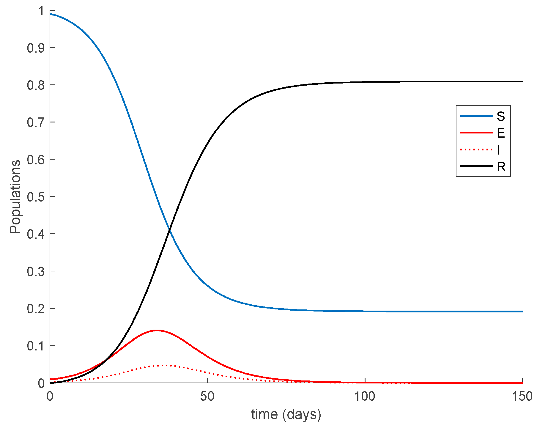
Case 1.1. There is no vaccination nor loss of immunity. It can be readily verified that the defined model satisfies Theorem 1 conditions, since

$$\mu \in \left(0\hspace{0.17em},\hspace{0.17em}1\right], \gamma \in \left(0\hspace{0.17em},\hspace{0.17em}1\right], \frac{\beta }{{\beta }^e}\le \frac{\gamma }{\mu }, \frac{\beta }{{\beta }^e}>0$$

(45)

and

$$0.5=S_0\le \frac{\mu }{2{\beta }^e}=0.5, 0.3=E_0\le \frac{\mu }{2{\beta }^e}=0.5, 0.1=I_0\le \frac{\mu }{2\beta }=0.17, R_0\ge 0$$

(46)

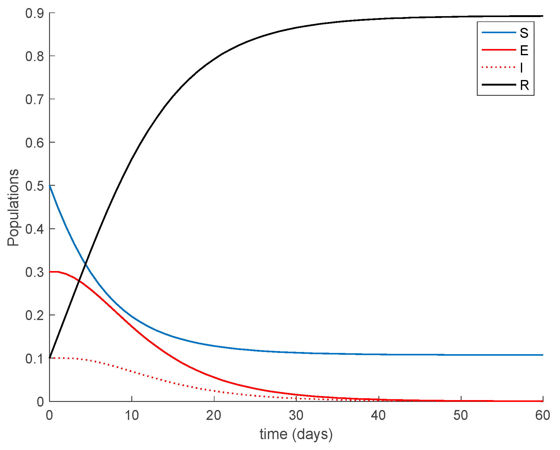
As a result of Theorem 1, all the sequences of populations are non-negative and bounded for all samples as Figure 1 shows. It is observed in Figure 1 that the system reaches a disease-free equilibrium point with a nonzero number of susceptible and immune individuals.

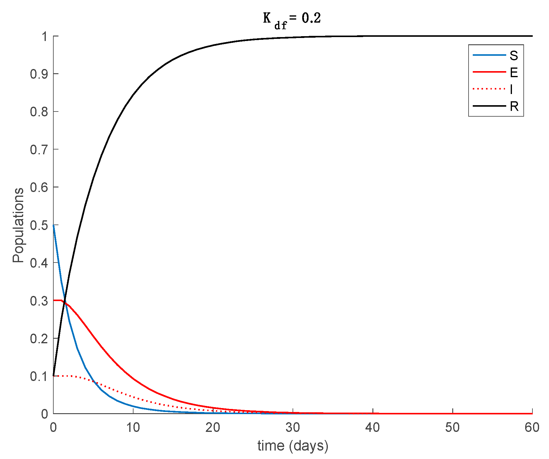
Case 1.2. There is vaccination but not loss of immunity. The vaccination gain is set to $K_{df}=0.2$ and $K_{df}=0.5$ to show the effect of this control action on the dynamics of the system. Since Theorem 1 conditions are still met, all the sequences of populations are non-negative and bounded for all time, as it can be seen in Figure 2 for both vaccination gains.

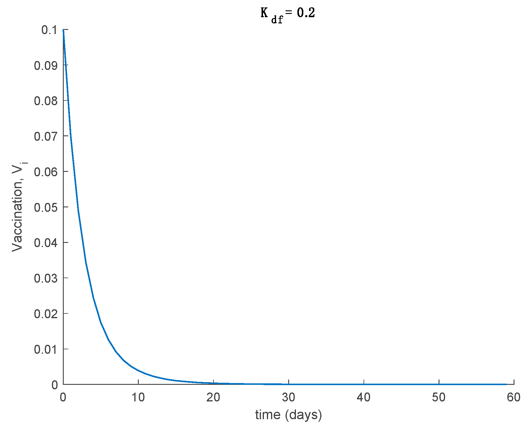
Moreover, it is observed in Figure 2 that the model converges to the disease-free equilibrium point given by the coordinates $S_{df}=E_{df}=I_{df}=0$, $R_{df}=1$ in both cases, as Proposition 1 predicts. It is also observed from Figure 1 and Figure 2 that the effect of vaccination when there is no loss of immunity is to make the whole population immune asymptotically while accelerating the convergence to the disease-free equilibrium point. The effect of changing the vaccination gain is slight; the susceptible vanish at a higher pace for larger values of the gain, while the shape of the exposed and infectious does not change significantly with vaccination. Figure 3 displays the vaccination function for both gains. As expected, a larger vaccination gain results in a higher vaccination control action.

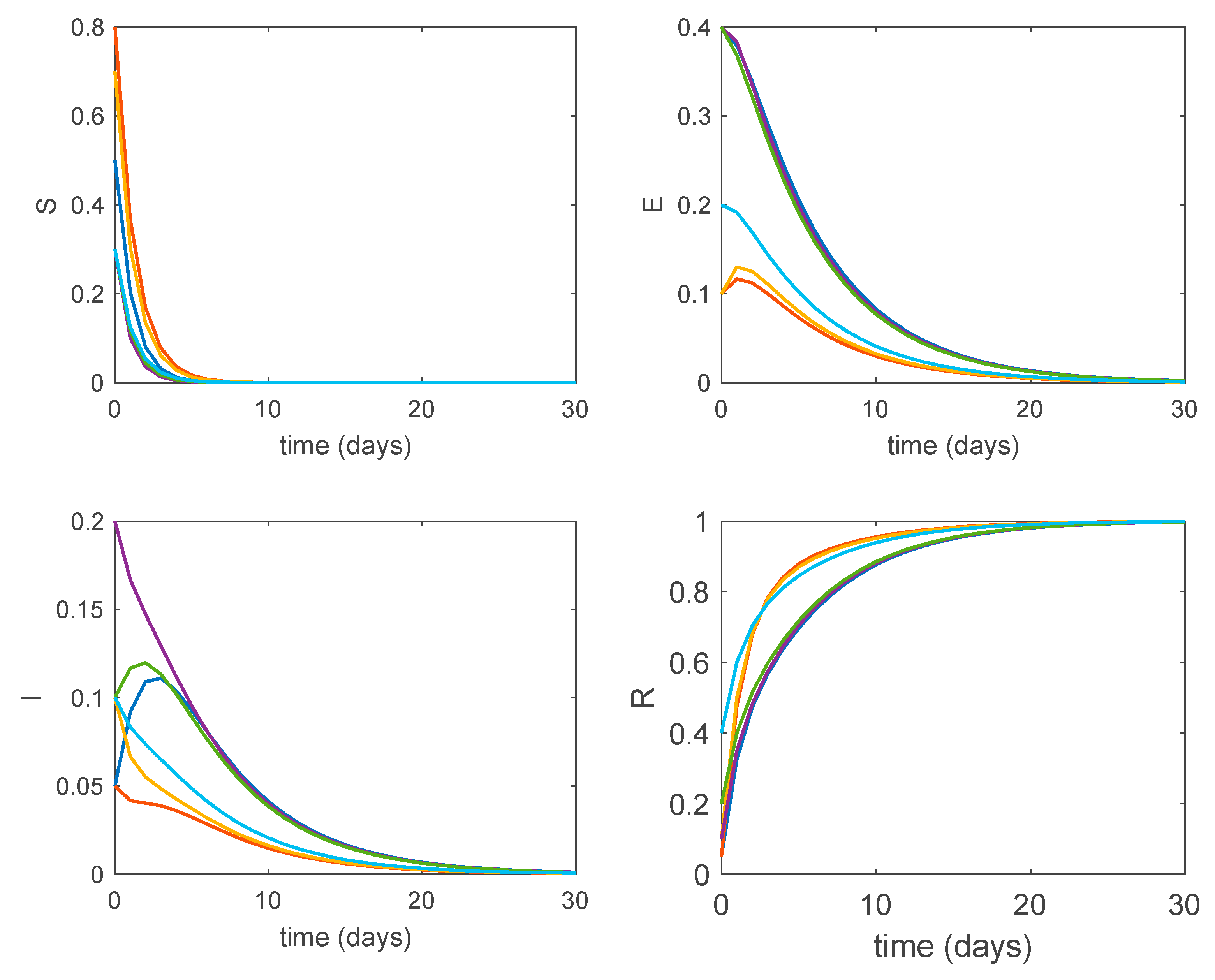
Furthermore, according to Theorem 3, the obtained disease-free equilibrium points are globally asymptotically stable. Figure 4 shows the dynamics of the system for perturbed initial conditions and $K_{df}=0.5$. It is seen in Figure 4 how all the system trajectories converge to the globally asymptotically stable disease-free equilibrium point regardless of the initial values.

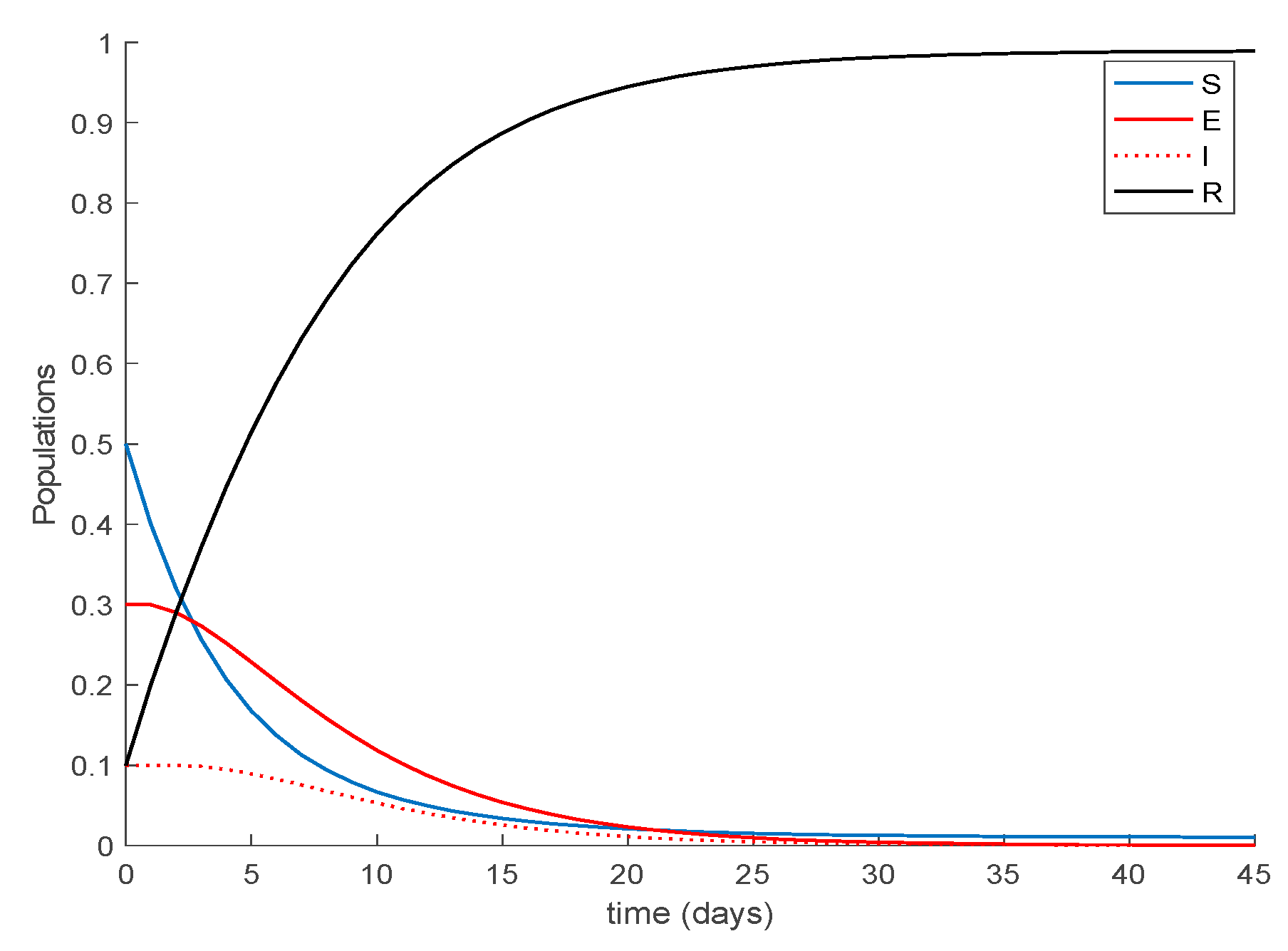
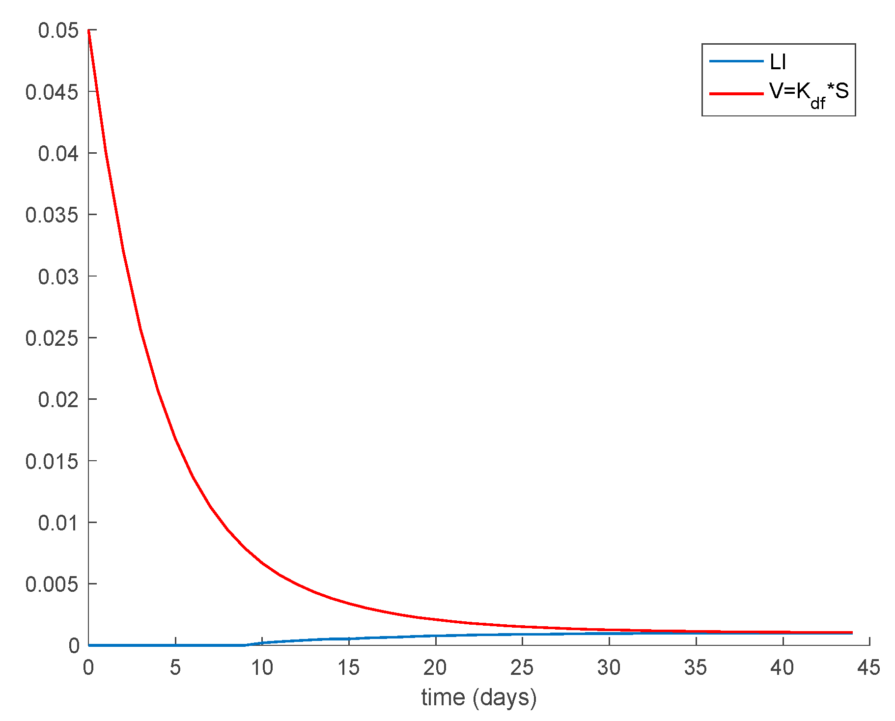
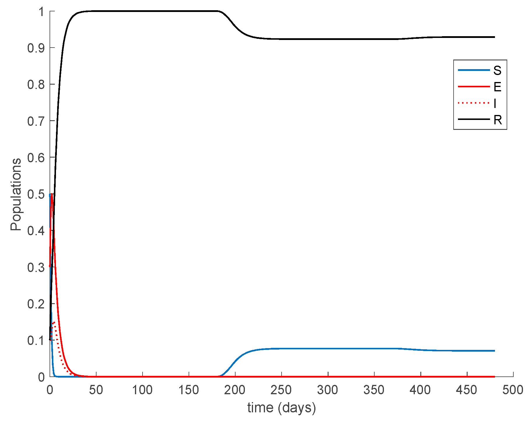
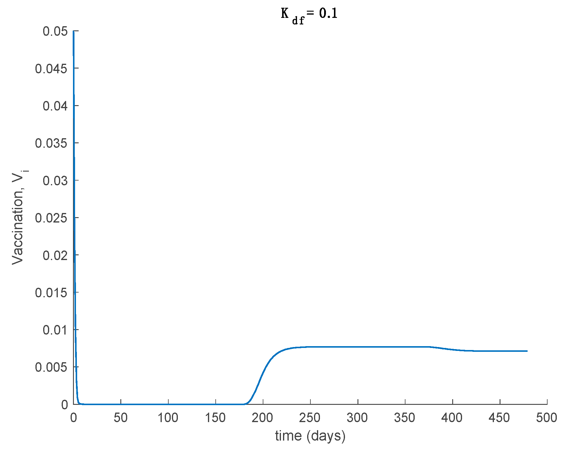
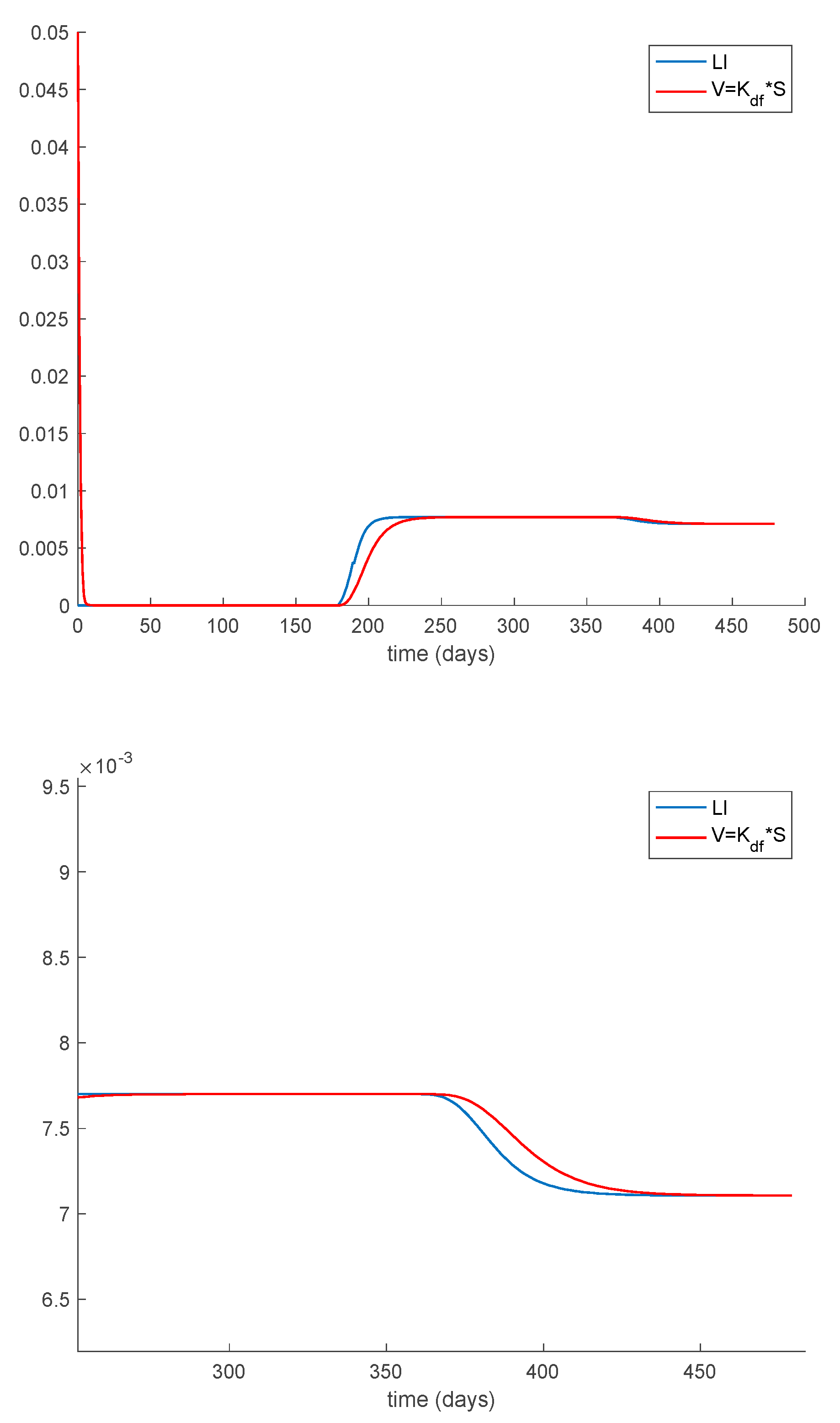
Case 1.3. The vaccination gain is set to $K_{df}=0.1$, and an exponentially fast partial loss of immunity with delay is considered. The parameters of the lost are given by $d_1=10$ and $d_2=5$ days and $\alpha =0.001$ with $A=0.001>0$. The dynamics of the system are depicted in Figure 5. Moreover, in addition to Conditions (1) and (2) from Theorem 1 we now need to check that Constraint (3) holds. This condition can be equivalently written as $LI\left({\hat{R}}_i\right)\le K_i{S}_i=V_i$. Figure 6 shows that this constraint is also met in this example so that all the population sequences are guaranteed to remain non-negative and bounded at all times, as is shown in Figure 5.

Furthermore, the system trajectories converge to the disease-free equilibrium point given by $S_{df}=\frac{A}{A+K_{df}}=0.0099$, $E_{df}=I_{df}=0$ and $R_{df}=\frac{K_{df}}{A+K_{df}}=0.9901$, in accordance with Proposition 1, which is globally asymptotically stable according to Theorem 3 since $\beta =0.5<{\beta }_c=25.225$ from (30).

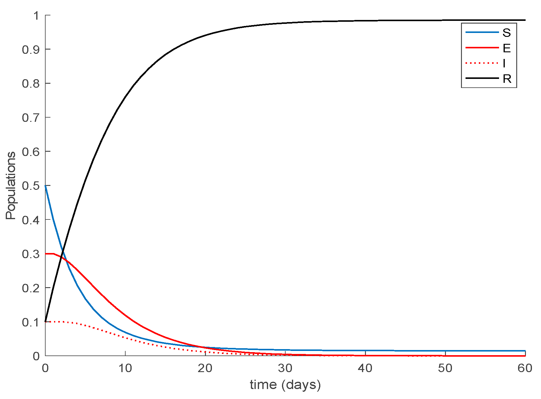
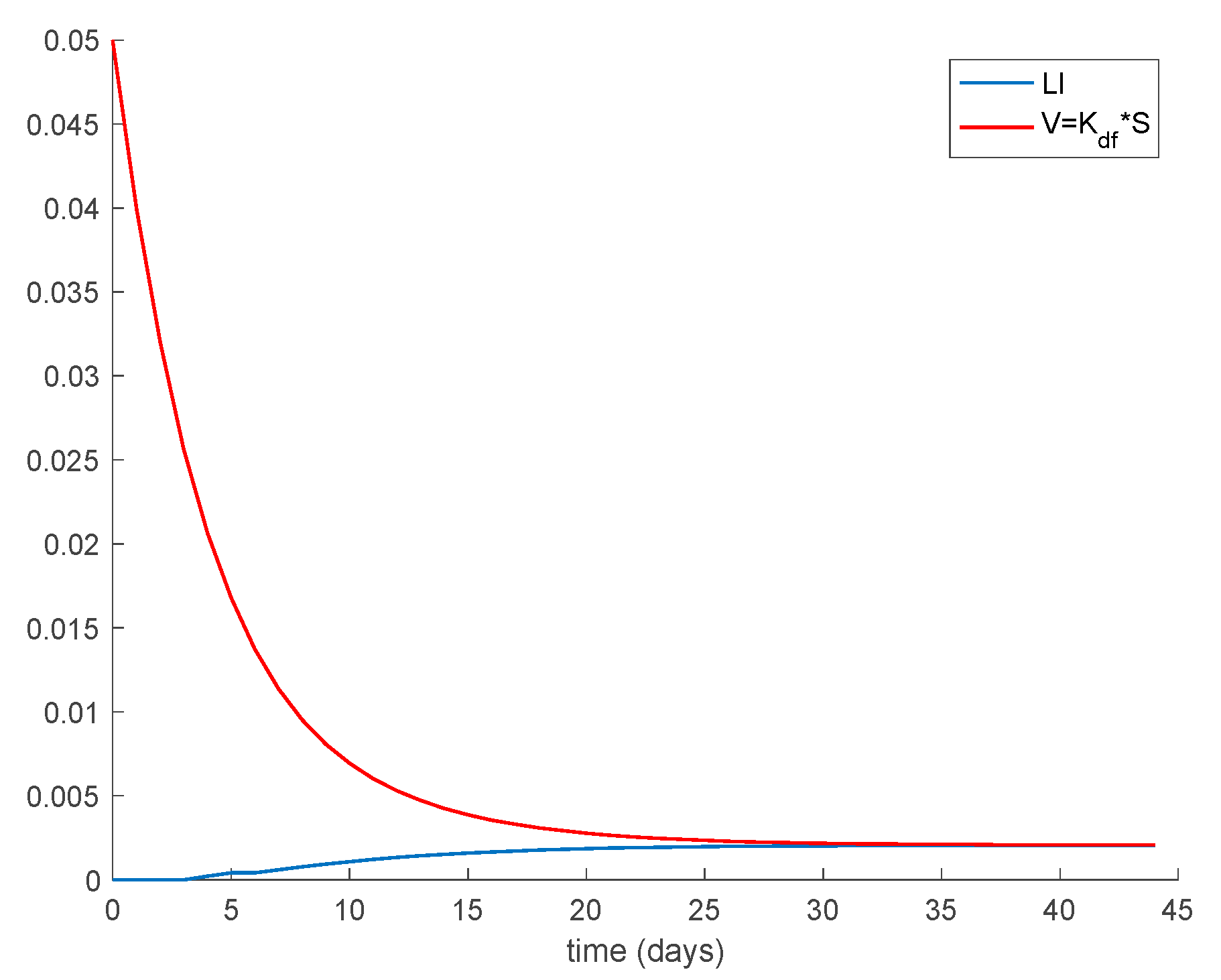
Case 1.4. The vaccination gain is set to $K_{df}=0.1$, and a constant loss of immunity with delay is considered. The parameters of the lost are given by $d_1=4$ and $d_2=2$ days and $a=0.0005$ with A = 0.0015. The dynamics of the system are depicted in Figure 7. As it happened before, in addition to Conditions (1) and (2) from Theorem 1 we need to check that Constraint (3) holds, which is performed in the same way as done for Case 1.3. Figure 8 depicts how Condition 3 from Theorem 1 is met. Furthermore, the system trajectories converge to the disease-free equilibrium point $S_{df}=\frac{A}{A+K_{df}}=0.0566$, $E_{df}=I_{df}=0$ and $R_{df}=\frac{K_{df}}{A+K_{df}}=0.9434$, which is globally asymptotically stable according to Theorem 3 since $\beta =0.5<{\beta }_c=3.5$ from (30).

Case 1.5. There is no vaccination nor loss of immunity, but the initial populations do not meet Theorem 1 conditions. This case is aimed at showing that the Theorem 1 conditions are sufficient to guarantee the boundedness and positivity of the populations but are not necessary. Thus, the following initial conditions are used in this case $S_0=0.99$, $E_0=0.01$, $I_0=0$ and $R_0=0$ for which $0.99=S_0>\frac{\mu }{2{\beta }^e}=0.5$, not satisfying Condition (2). The dynamics of the system are displayed in Figure 9. As it can be observed in Figure 9 all populations remain nonnegative and bounded for all time. In addition, the disease-free equilibrium point is also globally asymptotically stable as Theorem 3 states.

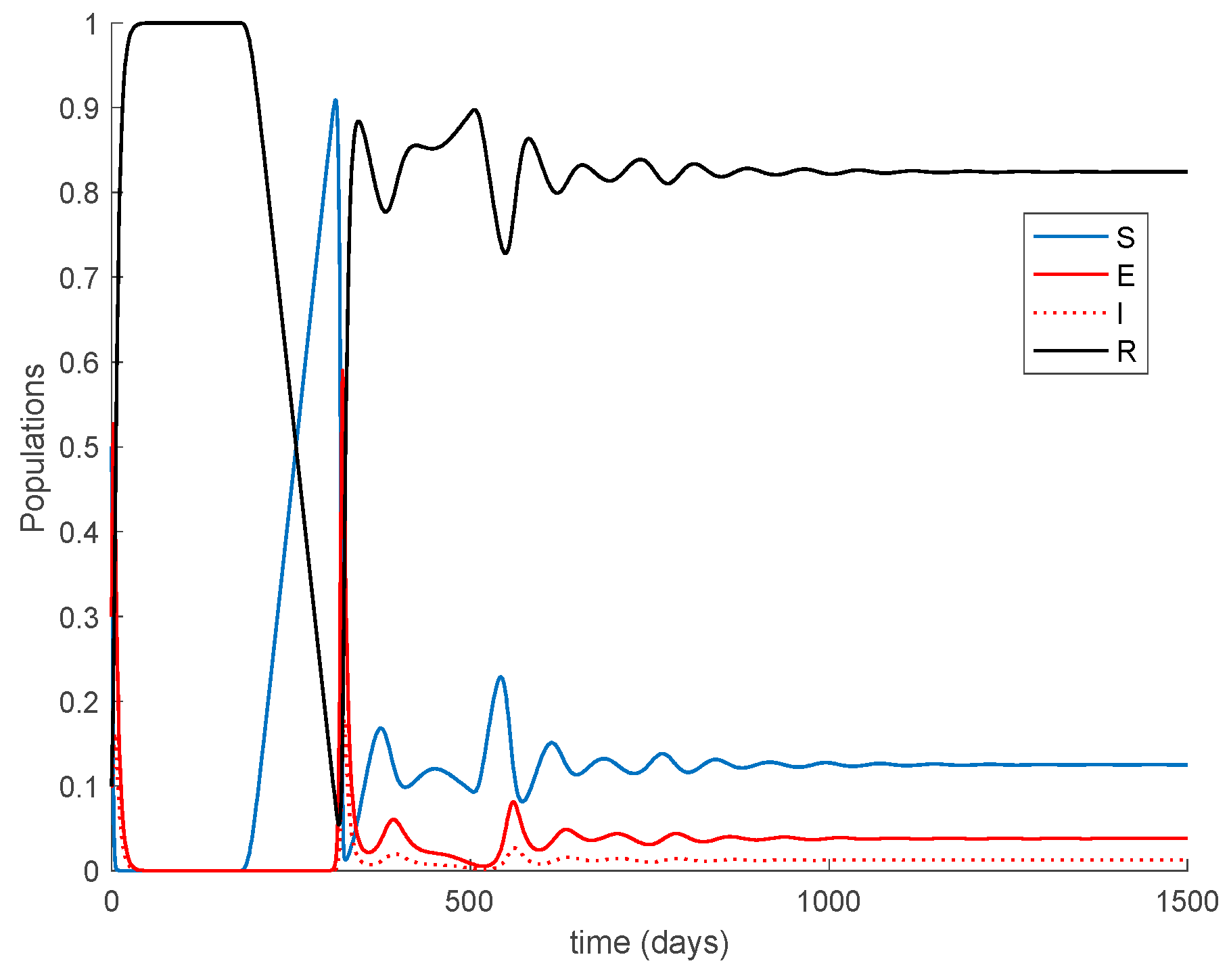
Case 1.6. There is no vaccination, and a constant loss of immunity with delay is considered. The parameters of the lost are given by $d_1=180$, $d_2=10$ days and $a=0.0007$ with A = 0.0077. The value of $\beta$ is increased to $\beta =2$ so that the endemic equilibrium point is now reachable and stable since $\beta =2>{\beta }_c=0.25$. The system trajectories are depicted in Figure 10.

It is observed in Figure 10 how after 180 days the loss of immunity makes some former immune individuals become susceptible again. In the end, an endemic equilibrium point is reached. From the numerical simulation we can obtain the location of the endemic equilibrium point and compare it with the theoretical values given in Proposition 2. The comparison is performed in

Table 1. Comparison of the theoretical values predicted by Proposition 2 and the numerically obtained ones for the location of the endemic point.

	Theoretical	Numerical
$S_{end}$	0.1250	0.1249
$E_{end}$	0.0381	0.0380
$I_{end}$	0.0127	0.0127
$R_{end}$	0.8242	0.8243

, which shows agreement between them.

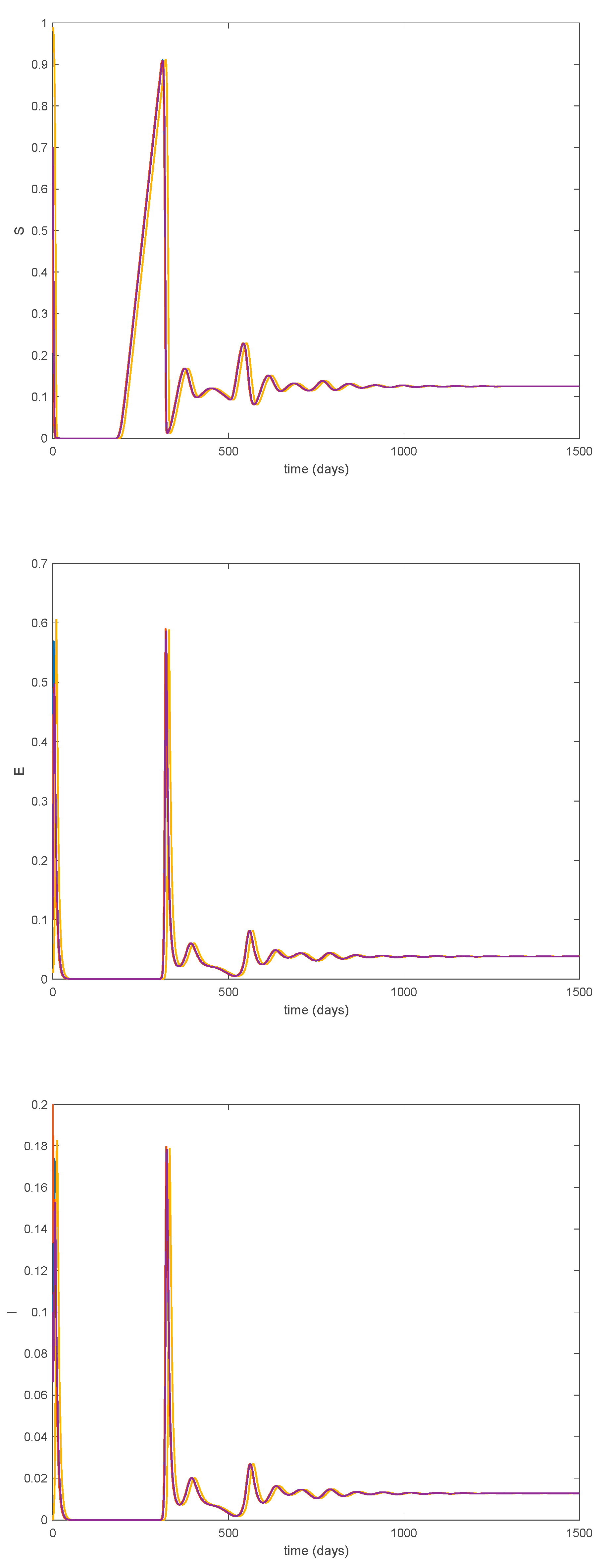
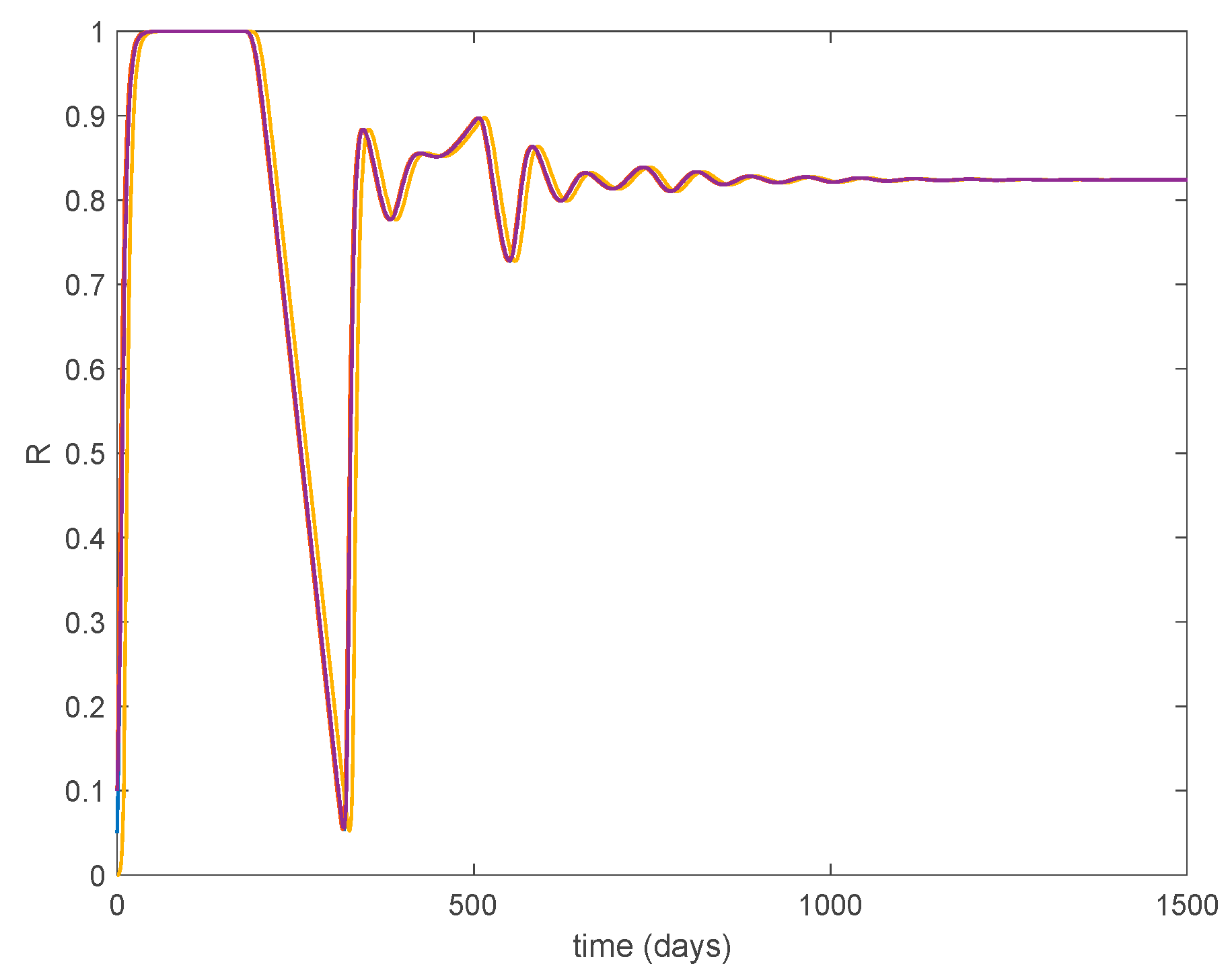
Furthermore, according to Theorem 5 the endemic equilibrium point is globally asymptotically stable, as Figure 11 shows for different initial conditions. Moreover, Figure 10 shows that the convergence to the endemic point exhibits a transient oscillation, but the trajectory does not have a steady-state periodic oscillation.

Case 1.7. The vaccination gain is $K_{df}=0.1$, and a constant loss of immunity with delay is considered. The parameters of the loss of immunity are given by $d_1=180$, $d_2=10$ days and $a=0.0007$ with A = 0.0077. The value of $\beta =2$ is used now as well. The system trajectories are depicted in Figure 12. It is observed in Figure 12 how the vaccination changes the dynamics of the system with respect to the vaccination-free case. Thus, vaccination is able to lessen the impact of loss of immunity so that the endemic equilibrium point is avoided and the system converges and remains in the disease-free equilibrium one. Therefore, the implementation of adequate vaccination campaigns throughout the year may act as a powerful tool to counteract the possibility of loss of immunity. This may be the case for the COVID-19 pandemic. Thus, Example 2 is devoted to study the application of the proposed model to COVID-19. From a mathematical point of view, the effect of vaccination is to change the critical beta value so that Condition (30) becomes $\beta =2>{\beta }_c=3.5$. Consequently, the disease-free equilibrium point is globally asymptotically stable while the endemic one is not reachable. Figure 13 displays the vaccination action to be applied through time. It is seen that vaccination does not vanish now asymptotically since it has to cope with the new susceptible appearing due to the loss of immunity. Finally, Theorem 3 requires the condition $\inf \hspace{0.17em}\left(K_i{S}_i-LI\left({\widehat{R}}_i\right)\right)\ge 0$ asymptotically in order to guarantee the global stability. This condition is shown in Figure 14. As it is observed in Figure 14 this condition may be violated within some time intervals, but it is achieved asymptotically. Thus, all conditions of Theorem 3 are achieved, and the disease-free equilibrium point is asymptotically stable.

5.2. Example 2. Application to the COVID-19 Pandemic

This example is devoted to study the application of the proposed model to the COVID-19 pandemic. To this end, the case of Italy will be considered. Thus, the model is parameterized by

$$\beta =0.2\hspace{0.17em},\hspace{1em}{\beta }^e=\frac{\beta }{1.3}\hspace{0.17em},\hspace{0.17em}\mu =\frac{1}{6}\hspace{0.17em},\hspace{0.17em}\gamma =0.04$$

while ${\lambda }^e=0.7692$. The sampling time is one day so that the units of the above parameters are in days⁻¹. The initial conditions are given by $S_0=240,000$, $E_0=0$, $I_0=240$ and $R_0=0$. These populations have been normalized to unity in the simulation examples, without loss of generality. The number of infectious, however, will be presented with actual data. This example has been divided into a number of cases in order to illustrate the dynamics of the model under different circumstances.

Case 2.1. There is no vaccination nor loss of immunity. Figure 15 displays the dynamics of the model along with the number of real cases reported in Italy from 26 February 2020 (which corresponds to the first day of simulation) for 145 consecutive days. This example for the COVID-19 pandemic has been considered previously in [31,32].

In the absence of loss of immunity, all the population becomes immune asymptotically. The following cases discuss the effects of loss of immunity and vaccination on the COVID-19 dynamics.

Case 2.2. There is no vaccination, and an exponentially fast loss of immunity with delay is considered. The parameters of the loss of immunity are given by $d_1=180$, $d_2=10$ days and $a=0.009$ with A = 0.0091. The dynamics of the models are depicted in Figure 16.

In Figure 16, a substantial change in the system dynamics due to the loss of immunity is observed. Therefore, the asymptotically stable disease-free equilibrium point gives way to an endemic equilibrium point, whose location is given by Proposition 2 as $S_{end}=0.1688$, $E_{end}=0.0353$, $I_{end}=0.1473$ and $R_{end}=0.6486$, in normalized units. Thus, in the steady-state there is always a number of infectious individuals. Moreover, the endemic equilibrium point is globally asymptotically stable since $\beta =0.2>{\beta }_c=0.034$ according to Theorem 5.

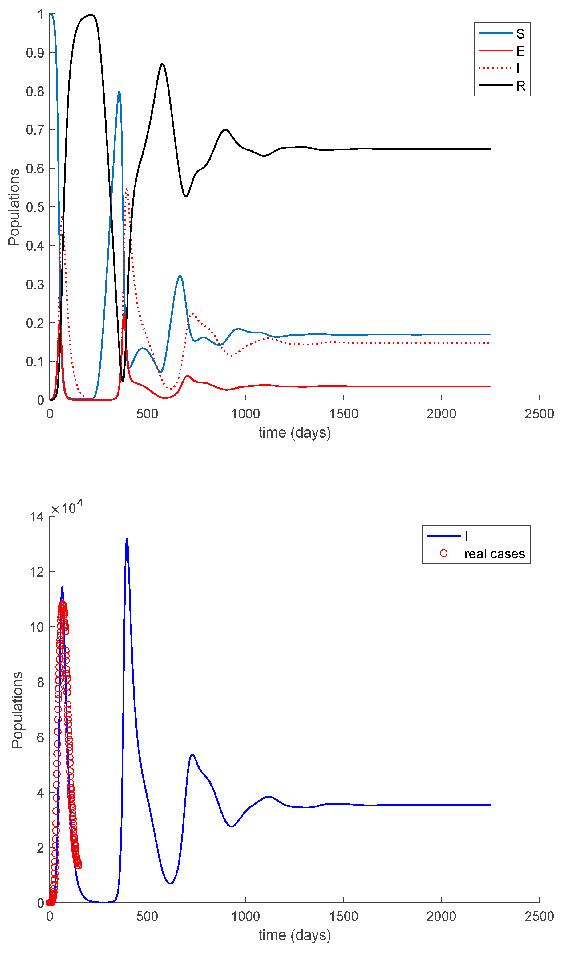
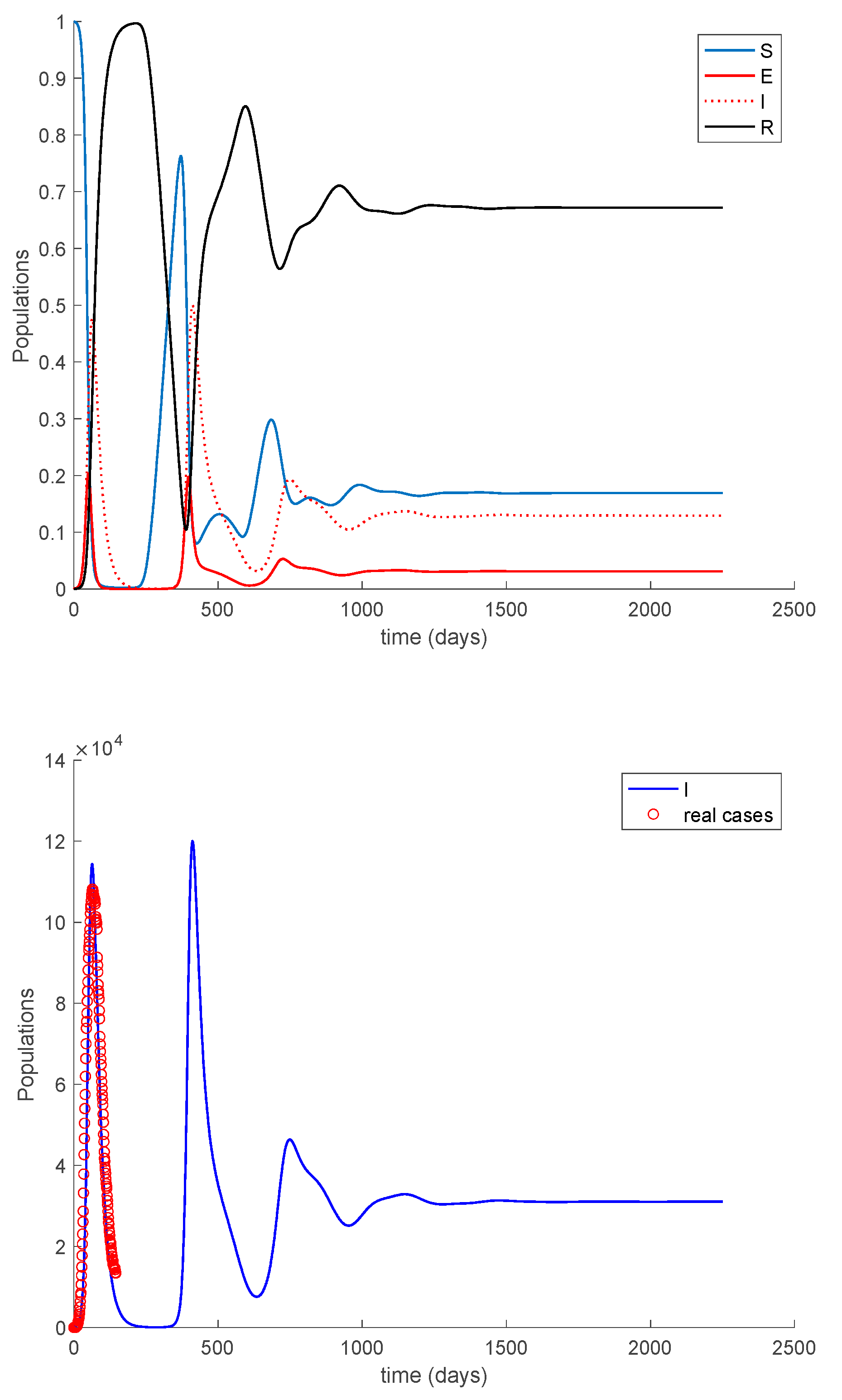
Case 2.3. There is no vaccination, and a constant loss of immunity with delay is considered. The parameters of the loss of immunity are given by $d_1=180$, $d_2=10$ days and $a=0.0007$ with A = 0.0077. The dynamics of the models are depicted in Figure 17.

As it happened in Case 2.2, the dynamics of the system changed substantially, and an endemic equilibrium point appears. This situation is not recommendable at all, and human intervention is necessary to avoid it. Consequently, the next Case 2.4 will study the effect of vaccination when loss of immunity occurs.

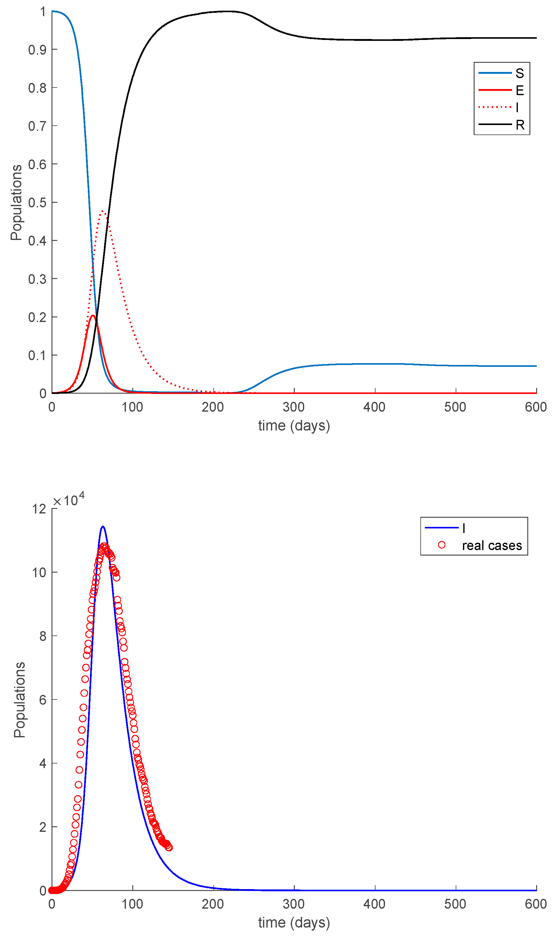
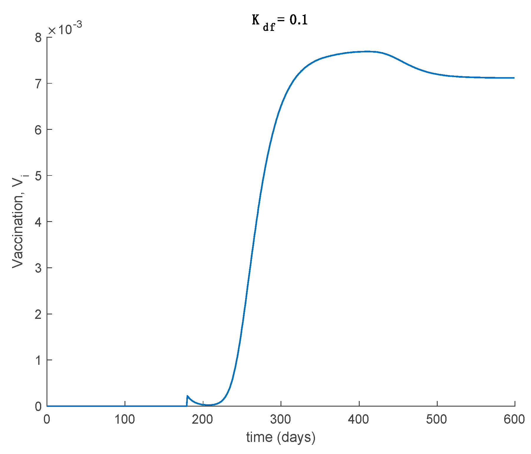
Case 2.4. The vaccination gain is $K_{df}=0.1$, and a constant loss of immunity with delay is considered. The parameters of the loss of immunity are given by $d_1=180$, $d_2=10$ days and $a=0.0007$ with A = 0.0077. The vaccination is only applied 180 days after the first day. This situation has been considered in order to discuss the effect of vaccination to counteract the loss of immunity. The dynamics of the system are depicted in Figure 18, while the vaccination is displayed in Figure 19.

It is deduced from Figure 18 that the vaccination, even with as low a percentage as 10%, allows avoiding the endemic state caused by the loss of immunity and makes the total population be either susceptible or immune asymptotically. The mathematical explanation for this is that vaccination generates a new critical value for beta so that $\beta =0.2<{\beta }_c=0.4723$. Therefore, the disease-free equilibrium point is globally asymptotically stable, while the endemic equilibrium point is no longer reachable. Overall, the proposed model is useful to describe the COVID-19 pandemic, study the effect of loss of immunity and assess the impact of vaccination in the epidemic spread.

6. Conclusions

A new discrete SEIR model has been presented in this paper subject to linear feedback vaccination controls on the susceptible and delayed partial loss of immunity of previously recovered individuals. It has also been considered that there is infectivity power in the Exposed-Susceptible contacts being, in general, of distinct transmission rate than that related to the Infectious-Susceptible contacts. The above idea is based on the knowledge that the later periods in the asymptomatic incubation phase of the infection in some infectious diseases, like for instance COVID-19, are also infective. It is considered that the partial loss of immunity in the recovered subpopulation increases the susceptibility after a certain delay depending on the period of the recovery immunity maintenance. Such an immunity loss is considered to take place in a range of samples previous to the current sample being active in the model, and both the duration of such a time interval where immunity is lost and the particular force per sample of such a loss can be adjusted with different weights in the proposed model to include the effect that the immunity loss is usually gradual through time. The proposed model considers also the use of feedback vaccination on the susceptible subpopulation. Furthermore, both the disease-free and the endemic equilibrium points are calculated explicitly as being dependent on the vaccination control gains. The stability of both equilibrium points is also discussed. It is proven that when the disease-free equilibrium point is asymptotically stable, the endemic one is not attainable, and when the endemic one is reachable then the disease-free one is unstable. In this way, it is proven that there is only a global attractor depending on the reproduction number or, equivalently, on its associate critical transmission rate. The proposed model has been tested through numerical examples based on COVID-19 parameterizations.

References

- Hethcote, H.W. The mathematics of infectious diseases. SIAM Rev. 2000, 42, 599–653. [Google Scholar] [CrossRef] [Green Version]
- Jiao, H.; Shen, Q. Dynamics Analysis and Vaccination-Based Sliding Mode Control of a More Generalized SEIR Epidemic Model. IEEE Access 2020, 8, 174507–174515. [Google Scholar] [CrossRef]
- De la Sen, M.; Ibeas, A.; Alonso-Quesada, S. On vaccination controls for the SEIR epidemic model. Commun. Nonlinear Sci. Numer. Simul. 2012, 17, 2637–2658. [Google Scholar] [CrossRef]
- De La Sen, M.; Nistal, R.; Ibeas, A.; Garrido, A.J. On the Use of Entropy Issues to Evaluate and Control the Transients in Some Epidemic Models. Entropy 2020, 22, 534. [Google Scholar] [CrossRef] [PubMed]
- Liu, F.; Huang, S.; Zheng, S.; O Wang, H. Stability Analysis and Bifurcation Control For a Fractional Order SIR Epidemic Model with Delay. In Proceedings of the 2020 39th Chinese Control Conference (CCC), Shenyang, China, 27–29 July 2020; pp. 724–729. [Google Scholar]
- Nistal, R.; De La Sen, M.; Alonso-Quesada, S.; Ibeas, A. On a New Discrete SEIADR Model with Mixed Controls: Study of Its Properties. Mathematics 2018, 7, 18. [Google Scholar] [CrossRef] [Green Version]
- Ibeas, A.; De La Sen, M.; Alonso-Quesada, S.; Nistal, R. Parameter Estimation of Multi-Staged SI(n)RS Epidemic Models. In Proceedings of the 2018 UKACC 12th International Conference on Control (CONTROL), Sheffield, UK, 5–7 September 2018; pp. 456–461. [Google Scholar]
- Wang, X.; Lu, J.; Wang, Z.; Li, Y. Dynamics of discrete epidemic models on heterogeneous networks. Phys. A Stat. Mech. Appl. 2020, 539, 122991. [Google Scholar] [CrossRef]
- Parsamanesh, M.; Mehrshad, S. Stability of the equilibria in a discrete-time sivs epidemic model with standard incidence. Filomat 2019, 33, 2393–2408. [Google Scholar] [CrossRef]
- Darti, I.; Suryanto, A.; Hartono, M. Global stability of a discrete SIR epidemic model with saturated incidence rate and death induced by the disease. Commun. Math. Biol. Neurosci. 2020, 2020. [Google Scholar] [CrossRef]
- Suryanto, A.; Darti, I. On the nonstandard numerical discretization of SIR epidemic model with a saturated incidence rate and vaccination. AIMS Math. 2021, 6, 141–155. [Google Scholar] [CrossRef]
- Shalan, R.N.; Shireen, R.; Lafta, A.H. Discrete an SIS model with immigrants and treatment. J. Interdiscip. Math. 2020, 1–6. [Google Scholar] [CrossRef]
- Córdova-Lepe, F.; Gutiérrez, R.; Vilches-Ponce, K. Analysis of two discrete forms of the classic continuous SIR epidemiological model. J. Differ. Equations Appl. 2019, 26, 1–24. [Google Scholar] [CrossRef]
- Radha, S.; Mahalakshmi, K.; Kumar, S.; Saravanakumar, A.R. E-learning during lockdown of COVID-19 pandemic: A global perspective. Int. J. Control Autom. 2020, 13, 1088–1089. [Google Scholar]
- Cao, H.; Wu, H.; Wang, X. Bifurcation analysis of a discrete SIR epidemic model with constant recovery. Adv. Differ. Equ. 2020, 2020, 1–20. [Google Scholar] [CrossRef]
- Youssef, H.M.; Alghamdi, N.A.; Ezzat, M.A.; El-Bary, A.A.; Shawky, A.M. A new dynamical modeling SEIR with global analysis applied to the real data of spreading COVID-19 in Saudi Arabia. Math. Biosci. Eng. 2020, 17, 7018–7044. [Google Scholar] [CrossRef] [PubMed]
- Alrashed, S.; Min-Allah, N.; Saxena, A.; Ali, I.; Mehmood, R. Impact of lockdowns on the spread of COVID-19 in Saudi Arabia. Informatics Med. Unlocked 2020, 20, 100420. [Google Scholar] [CrossRef]
- De La Sen, M.; Ibeas, A.; Agarwal, R.P. On Confinement and Quarantine Concerns on an SEIAR Epidemic Model with Simulated Parameterizations for the COVID-19 Pandemic. Symmetry 2020, 12, 1646. [Google Scholar] [CrossRef]
- De la Sen, M.; Ibeas, A. On a controlled SE (Is)(Ih)(Iicu) AR epidemic model with output controllability issues to satisfy hospital constraints on hospitalized patients. Algorithms 2020, 13, 322. [Google Scholar] [CrossRef]
- Zhai, S.; Gao, H.; Luo, G.; Tao, J. Control of a multigroup COVID-19 model with immunity: Treatment and test elimination. Nonlinear Dyn. 2020, 1–15. [Google Scholar] [CrossRef]
- Abbasi, Z.; Zamani, I.; Mehra, A.H.A.; Shafieirad, M.; Ibeas, A. Optimal Control Design of Impulsive SQEIAR Epidemic Models with Application to COVID-19. Chaos Solitons Fractals 2020, 139, 110054. [Google Scholar] [CrossRef] [PubMed]
- Etxeberria-Etxaniz, M.; Alonso-Quesada, S.; De La Sen, M. On an SEIR Epidemic Model with Vaccination of Newborns and Periodic Impulsive Vaccination with Eventual On-Line Adapted Vaccination Strategies to the Varying Levels of the Susceptible Subpopulation. Appl. Sci. 2020, 10, 8296. [Google Scholar] [CrossRef]
- Rohith, G.; Devika, K.B. Dynamics and control of COVID-19 pandemic with nonlinear incidence rates. Nonlinear Dyn. 2020, 101, 2013–2026. [Google Scholar] [CrossRef]
- Singh, R.K.; Drews, M.; De La Sen, M.; Kumar, M.; Singh, S.S.; Pandey, A.K.; Srivastava, P.K.; Dobriyal, M.; Rani, M.; Kumari, P.; et al. Short-Term Statistical Forecasts of COVID-19 Infections in India. IEEE Access 2020, 8, 186932–186938. [Google Scholar] [CrossRef]
- Tuite, A.R.; Ng, V.; Rees, E.; Fisman, D. Estimation of COVID-19 outbreak size in Italy. Lancet Infect. Dis. 2020, 20, 537. [Google Scholar] [CrossRef] [Green Version]
- Dutta, A. Stabilizing COVID-19 Infections in US by Feedback Control based Test and Quarantine. In Proceedings of the 2020 IEEE Global Humanitarian Technology Conference (GHTC), Seattle, WA, USA, 29 October–1 November 2020; pp. 300–305. [Google Scholar]
- Casella, F. Can the COVID-19 pandemic be controlled on the basis of daily test reports? IEEE Control Syst. Lett. 2021, 5, 1079–1084. [Google Scholar] [CrossRef]
- Paul, S.; Lorin, E. Lockdown: A non-pharmaceutical policy to prevent the spread of COVID-19. Math. Modeling Comput. Res. 2020. [Google Scholar] [CrossRef]
- Balabdaoui, F.; Dirk, M. Age-stratified discrete compartment model of the COVId-19 epidemic with application to Switzerland. Sci. Rep. 2020, 10, 2306. [Google Scholar] [CrossRef]
- Costa, J.A., Jr.; Martinez, A.C.; Geromel, J.C. On an alternative susceptible-infected removed epidemic model in discrete-time. Soc. Bras. Autom. 2020, 2, 2020. [Google Scholar] [CrossRef]
- Cooper, I.; Mondal, A.; Antonopoulos, C.G. A SIR model assumption for the spread of COVID-19 in different communities. Chaos Solitons Fractals 2020, 139, 110057. [Google Scholar] [CrossRef] [PubMed]
- De la Sen, M.; Ibeas, A. On a Sir epidemic model for the COVID-19 pandemic and the logistic equation. Discret. Dyn. Nat. Soc. 2020, 2020, 17. [Google Scholar] [CrossRef]
- Wang, Y.; Wei, Z.; Cao, J. Epidemic dynamics of influenza-like diseases spreading in complex networks. Nonlinear Dyn. 2020, 101, 1–20. [Google Scholar] [CrossRef]
- Wang, Y.; Cao, J. Final size of network epidemic models: Properties and connections. Sci. China Inf. Sci. 2020, 64, 1–3. [Google Scholar] [CrossRef]
- Chinwenyi, H.C.; Ibrahim, H.D.; Adekunle, J.O. A study of two disease models: With and without incubation period. Int. J. Math. Comput. Sci. 2019, 13, 74–79. [Google Scholar]
- Ng, K.Y.; Gui, M.M. COVID-19: Development of a robust mathematical model package with consideration for ageing population and time delay for control action and resusceptibility. Phys. D Nonlinear Phenom. 2010, 114, 132599. [Google Scholar]
- Ng, M.K.Y. SEIRS-Based COVID-19 Simulation Packge. Available online: https://www.markusng.com/COVIDSiM/ (accessed on 10 February 2021).
- Anderez, D.O.; Kanjo, E.; Pogrebna, G.; Kaiwartya, O.; Johnson, S.D.; Hunt, J.A. A COVID-19-Based Modified Epidemiological Model and Technological Approaches to Help Vulnerable Individuals Emerge from the Lockdown in the UK. Sensors 2020, 20, 4967. [Google Scholar] [CrossRef] [PubMed]
- Dobbs, P.S.; Watts, D.J. A generalized model of social and biological contagion. J. Theor. Biol. 2005, 232, 587–604. [Google Scholar]
Figure 1.
Sequences of populations for Case 1.1 conditions.
Figure 2.
Sequences of populations for Case 1.2 conditions. The vaccination gains and are employed in this simulation.
Figure 3.
Vaccination control action for and .
Figure 4.
Sequences of populations for Case 1.2 conditions, and perturbed initial values.
Figure 5.
Sequences of populations for Case 1.3 conditions. The vaccination gain is employed in this simulation with exponentially fast partial loss of immunity with delay.
Figure 6.
Satisfaction of Condition 3 from Theorem 1 in Case 1.3 conditions.
Figure 7.
Sequences of populations for Case 1.4 conditions. The vaccination gain is employed in this simulation with constant loss of immunity with delay.
Figure 8.
Satisfaction of Condition 3 from Theorem 1 in Case 1.4 conditions.
Figure 9.
Sequences of populations for Case 1.5 conditions.
Figure 10.
Sequences of populations for Case 1.6 conditions.
Figure 11.
Global asymptotical stability of the endemic equilibrium point for Case 1.6 conditions.
Figure 12.
Sequences of populations for Case 1.7 conditions.
Figure 13.
Vaccination action for Case 1.7 conditions.
Figure 14.
Condition to guarantee the global asymptotic stability of the disease-free equilibrium point for Case 1.7.
Figure 15.
Dynamics of the model for the COVID-19 pandemic in Italy for Case 2.1.
Figure 16.
Dynamics of the model for the COVID-19 pandemic in Italy for Case 2.2. There is no vaccination, and there is an exponentially fast loss of immunity with delay.
Figure 17.
Dynamics of the model for the COVID-19 pandemic in Italy for Case 2.3. There is no vaccination, and there is a constant loss of immunity with delay.
Figure 18.
Model dynamics with vaccination and a constant loss of immunity with delay. The vaccination gain is set to and it is applied after 180 days.
Figure 19.
Vaccination for Case 2.4, where a constant loss of immunity with delay is considered. The vaccination gain is set to and it is applied after 180 days.