Fractional System of Korteweg-De Vries Equations via Elzaki Transform

Abstract

In this article, a hybrid technique, called the Iteration transform method, has been implemented to solve the fractional-order coupled Korteweg-de Vries (KdV) equation. In this method, the Elzaki transform and New Iteration method are combined. The iteration transform method solutions are obtained in series form to analyze the analytical results of fractional-order coupled Korteweg-de Vries equations. To understand the analytical procedure of Iteration transform method, some numerical problems are presented for the analytical result of fractional-order coupled Korteweg-de Vries equations. It is also demonstrated that the current technique’s solutions are in good agreement with the exact results. The numerical solutions show that only a few terms are sufficient for obtaining an approximate result, which is efficient, accurate, and reliable.

1. Introduction

The engineering and physical systems that are best represented by fractional differential equations are described by fractional calculus (FC). Unfortunately, in many cases, the standard mathematical models of integer-order derivatives, including nonlinear models, do not work adequately. FC has played a very crucial role in different areas, such as chemistry, economics, electricity, notably control theory, groundwater problems, mechanics, signal image processing, and biology. Earlier, the study of travelling-wave solutions for non-linear equations played a significant role in analyzing non-linear physical processes. The KdV equation has defined a wide variety of physical phenomena used to model the interaction and evolution of non-linear waves [1,2,3,4,5,6,7,8].

Hirota and Satsuma suggested a coupled KdV model, which explains two long waves’ interactions with separate dispersion relationships. It was derived as an evolution equation governing a one-dimensional, small-amplitude, and long-surface gravity wave propagating in a shallow channel of water. The non-linear coupled scheme of partial differential equations (PDEs) has a wide range of implementations in different fields of chemistry, biology, hydrodynamics, mechanics, plasma physics, water waves, applied science, etc. In [9], Wu et al. introduced a novel hierarchy of non-linear equations of evolution by considering a spectral $4\times 4$ matrix problem with three potentials. However, the behavior of the KdV solitons recognizes the influence of the existence of the former. The result shows that the former defines the velocity of the KdV soliton [10,11]. The fractional-order coupled KdV equations are defined as

$$\begin{array}{cc}\hfill & \frac{{\partial }^{\rho }\mu }{\partial {\tau }^{\rho }}=-a\frac{{\partial }^3\mu }{\partial {\zeta }^3}-6a\mu \frac{\partial \mu }{\partial \zeta }+6\nu \frac{\partial \nu }{\partial \zeta }\hfill \\ \hfill & \frac{{\partial }^{\rho }\nu }{\partial {\tau }^{\rho }}=-a\frac{{\partial }^3\nu }{\partial {\zeta }^3}-3b\mu \frac{\partial \nu }{\partial \zeta },0<\rho <1\hfill \end{array}$$

(1)

where a and b are constants and $\rho$ is a parameter describing the order of the fractional-order derivatives of $\mu (\zeta ,\tau )$ and $\nu (\zeta ,\tau )$, respectively. The functions $\mu (\zeta ,\tau )$ and $\nu (\zeta ,\tau )$ are considered to be the fundamental functions of space and time, i.e., disappearing for $\tau <0$ and $\zeta <0$. Because $a=b=1$ is used, the latter scheme reduces to the classical coupled KdV equations.

The modified coupled Koreweg-de Vries system (MCKdV) is a typical equation in this hierarchy. This equation is governed by the following non-linear PDEs [12]:

$$\begin{array}{cc}\hfill \frac{{\partial }^{\rho }\mu }{\partial {\tau }^{\rho }}& =\frac{1}{2}\frac{{\partial }^3\mu }{\partial {\tau }^3}-3{\mu }^2\frac{\partial \mu }{\partial \zeta }+\frac{3}{2}\omega \frac{{\partial }^2\nu }{\partial {\zeta }^2}+3\frac{\partial \nu }{\partial \zeta }\frac{\partial \omega }{\partial \zeta }+\frac{3}{2}\nu \frac{{\partial }^2\omega }{\partial {\zeta }^2}+3\nu \omega \frac{\partial \mu }{\partial \zeta }+3\mu \omega \frac{\partial \nu }{\partial \zeta }+3\mu \nu \frac{\partial \omega }{\partial \zeta },\hfill \\ \hfill \frac{{\partial }^{\rho }\nu }{\partial {\tau }^{\rho }}& =-\frac{{\partial }^3\nu }{\partial {\zeta }^3}-3\frac{\partial \mu }{\partial \zeta }\frac{\partial \nu }{\partial \zeta }-3\nu \frac{{\partial }^2\mu }{\partial {\zeta }^2}-3{\nu }^2\frac{\partial \omega }{\partial \zeta }+6\mu \nu \frac{\partial \mu }{\partial \zeta }+3{\mu }^2\frac{\partial \nu }{\partial \zeta },\hfill \\ \hfill \frac{{\partial }^{\rho }\omega }{\partial {\tau }^{\rho }}& =-\frac{{\partial }^3\omega }{\partial {\zeta }^3}-3\frac{\partial \mu }{\partial \zeta }\frac{\partial \omega }{\partial \zeta }-3\omega \frac{{\partial }^2\mu }{\partial {\zeta }^2}-3{\omega }^2\frac{\partial \nu }{\partial \zeta }+6\mu \omega \frac{\partial \mu }{\partial \zeta }+3{\mu }^2\frac{\partial \omega }{\partial \zeta },\hfill \end{array}$$

(2)

The MCKdV Equation (2), with $\nu =\omega =0$, reduces to the standard modified KdV equation. KdV equations are a major class of non-linear evolution equations with several implementations in engineering and applied sciences. As an example, in plasma physics, the KdV equations result in the ion acoustic solutions [13,14]. A long wave characterizes geophysical fluid dynamics in shallow waters and deep oceans [15,16].

The solution of the Generalized Hirota–Satsuma coupled KdV equations has been achieved by the Adomian decomposition technique [17]. An exact solution has suggested the result of coupled KdV, while using the homogenous balance technique. By applying differential transform technique, the approximate result of coupled KdV has been studied in [18]. The analysis of non-linear KdV equations suggested in [19] was using the Homotopy analysis method. The exact result of KdV has been found through the analysis in [20] applying the variational iteration technique. Lu, D et al. found the numerical solutions of coupled nonlinear fractional KdV equations using Fractional Elzaki projected differential transform method [21]. The approximate results for a generalized coupled scheme of KdV and Zakharov–Kuznetsov equations have been achieved in [22] while using a modified tanh technique. Fan [23] have employed an extended tanh technique with symbolic computation to derive the rational results, periodic triangular results and soliton results of the MCKdV scheme of equations. This method’s basic concept is to use a Riccati equation involving a parameter, and then apply its effects to replace the tanh-function in the tanh technique. Cavlak and Inc, in [24], applied the variational iteration technique and Adomian decomposition technique to obtain analytical results of the MCKdV scheme of equations. The homotopy analysis technique has also been used on the MCKdV system of equations in [25,26].

In 2006, Daftardar-Gejji and Jafari introduced a new iterative methodology for the mathematical solution of non-linear equations [27]. Jafari et al. first applied the Laplace transform in the iterative method. They proposed a new straightforward method, called iterative Laplace transform method (ILTM) [28], to look for numerical effects of the FPDE system. ILTM was used to solve linear and non-linear PDEs, such as fractional-order Fokker Planck equations [29], time-fractional Zakharov Kuznetsov equation [30], and fractional-order Fornberg Whitham equation [31], etc. Because we know that the Elzaki transformation is the generalization of Laplace and Sumudu transformations, it can contribute in a similar way as Laplace and Sumudu transformations to determine the analytical solutions of the differential equations. Elzaki Transform is derived from the classical Fourier integral, based on the mathematical simplicity of the Elzaki transform and its fundamental properties. Elzaki transform was introduced by Tarig ELzaki to facilitate the process of solving ordinary and partial differential equations in the time domain. Typically, Fourier, Laplace, and Sumudu transforms are the convenient mathematical tools for solving differential equations. It should be noted that the Elzaki transformation was initially chosen to successfully compete with an older and more developed method, like the Sumudu method. However, so far, we have not proved that Elzaki transformation is able to solve problems cannot be solved by Laplace [32]. In this paper, the iterative technique is modified with the Elzaki transform, and the new method is called New Iterative transformation method.

The new iterative transform method is implemented to investigated fractional-order of the system of KDV equations. The result of certain illustrative cases is discussed to explain the feasibility of the suggested method. The results for fractional-order models, as well as integral-order models, are determined using the current techniques. The suggested method is also constructive for addressing other fractional orders of linear and non-linear PDEs.

2. Basic Preliminaries

Definition 1.

The Riemann–Liouville of fractional operator $D^{\rho }$ of order ρ is given as [33,34]

$$D^{\rho }\nu \left(\zeta \right)=\left\{\begin{array}{c}\frac{d^j}{d{\zeta }^j}\nu \left(\zeta \right),\rho =j\hfill \\ \frac{1}{{\Gamma }(j-\rho )}\frac{d}{d{\zeta }^j}{\int }_0^{\zeta }\frac{\nu \left(\zeta \right)}{{(\zeta -\psi )}^{\rho -j+1}}d\psi ,j-1<\rho <j\hfill \end{array}\right.$$

where $j\in Z^{+}$, $\rho \in R^{+}$ and

$$D^{\rho }\nu \left(\zeta \right)=\frac{1}{{\Gamma }\left(\rho \right)}{\int }_0^{\zeta }{(\zeta -\psi )}^{\rho -1}\nu \left(\psi \right)d\psi ,0<\rho \le 1.$$

Definition 2.

The fractional-order Riemann–Liouville integration operator $J^{\rho }$ is defined as [33,34]

$$J^{\rho }\nu \left(\zeta \right)=\frac{1}{{\Gamma }\left(\rho \right)}{\int }_0^{\zeta }{(\zeta -\psi )}^{\rho -1}\nu \left(\zeta \right)d\zeta ,\zeta >0,\rho >0.$$

The basic properties of the operator

$$\begin{array}{c}\hfill J^{\rho }{\zeta }^j=\frac{{\Gamma }(j+1)}{{\Gamma }(j+\rho +1)}{\zeta }^{j+\rho }\\ \hfill D^{\rho }{\zeta }^j=\frac{{\Gamma }(j+1)}{{\Gamma }(j-\rho +1)}{\zeta }^{j-\rho }\end{array}$$

Definition 3.

The Caputo fractional operator $D^{\rho }$ of ρ is defined as [33,34]

$${}^C{D}^{\rho }\nu \left(\zeta \right)=\left\{\begin{array}{c}\frac{1}{{\Gamma }(j-\rho )}{\int }_0^{\zeta }\frac{{\nu }^j\left(\psi \right)}{{(\zeta -\psi )}^{\rho -j+1}}d\psi ,j-1<\rho <j,\hfill \\ \frac{d^j}{d{\zeta }^j}\nu \left(\zeta \right),j=\rho .\hfill \end{array}\right.$$

(3)

Definition 4.

$$\begin{array}{cc}\hfill J_{\zeta }^{\rho }{D}_{\zeta }^{\rho }g\left(\zeta \right)& =g\left(\zeta \right)-\sum _{k=0}^m{g}^k\left(0^{+}\right)\frac{{\zeta }^k}{k!},for\zeta >0,andj-1<\rho \le j,j\in N.\hfill \\ \hfill D_{\zeta }^{\rho }{J}_{\zeta }^{\rho }g\left(\zeta \right)& =g\left(\zeta \right)\hfill \end{array}$$

(4)

Definition 5.

The fractional-order Caputo operator of Elzaki transform is given as:

$$E\left[D_{\zeta }^{\rho }g\left(\zeta \right)\right]=s^{-\rho }E\left[g\left(\zeta \right)\right]-\sum _{k=0}^{j-1}{s}^{2-\rho +k}{g}^{\left(k\right)}\left(0\right),wherej-1<\rho <j.$$

3. The General Methodology of New Iterative Transform Method (NITM)

Consider the general form of fractional partial differential equation.

$$D_{\tau }^{\rho }\upsilon (\zeta ,\tau )+M\upsilon (\zeta ,\tau )+N\upsilon (\zeta ,\tau )=h(\zeta ,\tau ),j\in N,j-1<\rho \le j,$$

(5)

where M and N are the linear and non-linear operators and h is a source function.

The initial condition is

$${\upsilon }^{\left(k\right)}(\zeta ,0)=g_k\left(\zeta \right),k=0,1,2,...,j-1,$$

(6)

implementing the Elzaki transformation of Equation (5), we obtain

$$E\left[D_{\tau }^{\rho }\upsilon (\zeta ,\tau )\right]+E[M\upsilon (\zeta ,\tau )+N\upsilon (\zeta ,\tau )]=E\left[h(\zeta ,\tau )\right].$$

(7)

Applying the Elzaki differentiation is given to

$$E\left[\upsilon (\zeta ,\tau )\right]=\sum _{k=0}^m{s}^{2-\rho +k}{\upsilon }^{\left(k\right)}(\zeta ,0)+s^{\rho }E\left[h(\zeta ,\tau )\right]-s^{\rho }E[M\upsilon (\zeta ,\tau )+N\upsilon (\zeta ,\tau )],$$

(8)

inverse Elzaki transform converts Equation (8) into

$$\upsilon (\zeta ,\tau )=E^{-1}\left[\left(\sum _{k=0}^m{s}^{2-\rho +k}{\upsilon }^k(\zeta ,0)+s^{\rho }E\left[h(\zeta ,\tau )\right]\right)\right]-E^{-1}\left[s^{\rho }E[M\upsilon (\zeta ,\tau )+N\upsilon (\zeta ,\tau )]\right].$$

(9)

As, through the iterative technique, we have

$$\upsilon (\zeta ,\tau )=\sum _{m=0}^{\infty }{\upsilon }_m(\zeta ,\tau ).$$

(10)

Further, the operator M is linear, therefore

$$M\left(\sum _{m=0}^{\infty }{\upsilon }_m(\zeta ,\tau )\right)=\sum _{m=0}^{\infty }M\left[{\upsilon }_m(\zeta ,\tau )\right],$$

(11)

and the operator N is nonlinear, we have the following

$$N\left(\sum _{m=0}^{\infty }{\upsilon }_m(\zeta ,\tau )\right)={\upsilon }_0(\zeta ,\tau )+N\left(\sum _{k=0}^m{\upsilon }_k(\zeta ,\tau )\right)-M\left(\sum _{k=0}^m{\upsilon }_k(\zeta ,\tau )\right).$$

(12)

Putting Equations (10)–(12) in Equation (9), we have achieve the following result

$$\begin{array}{cc}\hfill & \sum _{m=0}^{\infty }{\upsilon }_m(\zeta ,\tau )=E^{-1}\left[s^{\rho }\left(\sum _{k=0}^m{s}^{2-\zeta +k}{\upsilon }^k(\zeta ,0)+E\left[h(\zeta ,\tau )\right]\right)\right]\hfill \\ \hfill & -E^{-1}\left[s^{\rho }E\left[M\left(\sum _{k=0}^m{\upsilon }_k(\zeta ,\tau )\right)-N\left(\sum _{k=0}^m{\upsilon }_k(\zeta ,\tau )\right)\right]\right].\hfill \end{array}$$

(13)

We define the below mentioned iterative formula while applying Equation

$${\upsilon }_0(\zeta ,\tau )=E^{-1}\left[s^{\rho }\left(\sum _{k=0}^m{s}^{2-\zeta +k}{\upsilon }^k(\zeta ,0)+s^{\rho }E\left(h(\zeta ,\tau )\right)\right)\right],$$

(14)

$${\upsilon }_1(\zeta ,\tau )=-E^{-1}\left[s^{\rho }E[M\left[{\upsilon }_0(\zeta ,\tau )\right]+N\left[{\upsilon }_0(\zeta ,\tau )\right]\right],$$

(15)

$$\begin{array}{cc}\hfill & {\upsilon }_{m+1}(\zeta ,\tau )=-E^{-1}\left[s^{\rho }E\left[-M\left(\sum _{k=0}^m{\upsilon }_k(\zeta ,\tau )\right)-N\left(\sum _{k=0}^m{\upsilon }_k(\zeta ,\tau )\right)\right]\right],m\ge 1\hfill \end{array}$$

(16)

Finally, the Equations (5) and (6) provide the m-term result in series form, given as

$$\upsilon (\zeta ,\tau )\cong {\upsilon }_0(\zeta ,\tau )+{\upsilon }_1(\zeta ,\tau )+{\upsilon }_2(\zeta ,\tau )+.....,+{\upsilon }_m(\zeta ,\tau ),m=1,2,\cdots .$$

(17)

4. Applications of the Proposed Method

Example 1.

Consider the fractional-order non-linear KdV system is given as

$$\begin{array}{cc}\hfill & \frac{{\partial }^{\rho }\mu }{\partial {\tau }^{\rho }}=-a\frac{{\partial }^3\mu }{\partial {\zeta }^3}-6a\mu \frac{\partial \mu }{\partial \zeta }+6\nu \frac{\partial \nu }{\partial \zeta }\hfill \\ \hfill & \frac{{\partial }^{\rho }\nu }{\partial {\tau }^{\rho }}=-a\frac{{\partial }^3\nu }{\partial {\zeta }^3}-3a\mu \frac{\partial \nu }{\partial \zeta },0<\rho <1\hfill \end{array}$$

(18)

with initial condition

$$\mu (\zeta ,0)={\eta }^{2}sec{h}^2\left(\frac{\alpha }{2}+\frac{\eta \zeta }{2}\right),\nu (\zeta ,0)=\sqrt{\frac{a}{2}}{\eta }^{2}sec{h}^2\left(\frac{\alpha }{2}+\frac{\eta \zeta }{2}\right).$$

(19)

For $\rho =1$, the exact results of the KdV scheme Equation (18) are given by

$$\begin{array}{cc}\hfill & \mu (\zeta ,\tau )={\eta }^{2}sec{h}^2\left(\frac{\alpha }{2}+\frac{\eta \zeta }{2}-\frac{a{\eta }^3\tau }{2}\right),\hfill \\ & \nu (\zeta ,\tau )=\sqrt{\frac{a}{2}}{\eta }^{2}sec{h}^2\left(\frac{\alpha }{2}+\frac{\eta \zeta }{2}-\frac{a{\eta }^3\tau }{2}\right),\hfill \end{array}$$

(20)

Using the Elzaki transform to Equation (18), we obtain

$$\begin{array}{cc}\hfill & \frac{1}{{\mathrm{s}}^{\rho }}E\left[\mu (\zeta ,\tau )\right]-\sum _{k=0}^{m-1}{\mu }_{\left(k\right)}(\zeta ,0){\mathrm{s}}^{2-\rho +k}=E\left[-a\frac{{\partial }^3\mu }{\partial {\zeta }^3}-6a\mu \frac{\partial \mu }{\partial \zeta }+6\nu \frac{\partial \nu }{\partial \zeta }\right],\hfill \\ \hfill & \frac{1}{{\mathrm{s}}^{\rho }}E\left[\nu (\zeta ,\tau )\right]-\sum _{k=0}^{m-1}{\upsilon }_{\left(k\right)}(\zeta ,0){\mathrm{s}}^{2-\rho +k}=E\left[-a\frac{{\partial }^3\nu }{\partial {\zeta }^3}-3a\mu \frac{\partial \nu }{\partial \zeta }\right],\hfill \\ \hfill & \frac{1}{{\mathrm{s}}^{\rho }}E\left[\mu (\zeta ,\tau )\right]={\mu }_{\left(0\right)}(\zeta ,0){\mathrm{s}}^{2-\rho }+E\left[-a\frac{{\partial }^3\mu }{\partial {\zeta }^3}-6a\mu \frac{\partial \mu }{\partial \zeta }+6\nu \frac{\partial \nu }{\partial \zeta }\right],\hfill \\ \hfill & \frac{1}{{\mathrm{s}}^{\rho }}E\left[\nu (\zeta ,\tau )\right]={\nu }_{\left(0\right)}(\zeta ,0){\mathrm{s}}^{2-\rho }+E\left[-a\frac{{\partial }^3\nu }{\partial {\zeta }^3}-3a\mu \frac{\partial \nu }{\partial \zeta }\right],\hfill \end{array}$$

(21)

$$\begin{array}{cc}\hfill E\left[\mu \right(\zeta ,\tau \left)\right]& ={\mathrm{s}}^2\mu (\zeta ,0)+{\mathrm{s}}^{\rho }E\left[-a\frac{{\partial }^3\mu }{\partial {\zeta }^3}-6a\mu \frac{\partial \mu }{\partial \zeta }+6\nu \frac{\partial \nu }{\partial \zeta }\right].\hfill \\ \hfill E\left[\nu \right(\zeta ,\tau \left)\right]& ={\mathrm{s}}^2\nu (\zeta ,0)+{\mathrm{s}}^{\rho }E\left[-a\frac{{\partial }^3\nu }{\partial {\zeta }^3}-3a\mu \frac{\partial \nu }{\partial \zeta }\right].\hfill \end{array}$$

(22)

Applying inverse Elzaki transform of Equation (22), we have

$$\begin{array}{cc}\hfill \mu (\zeta ,\tau )& =E^{-1}\left[{\mathrm{s}}^2\mu (\zeta ,0)\right]+E^{-1}\left[{\mathrm{s}}^{\rho }E\left(-a\frac{{\partial }^3\mu }{\partial {\zeta }^3}-6a\mu \frac{\partial \mu }{\partial \zeta }+6\nu \frac{\partial \nu }{\partial \zeta }\right)\right].\hfill \\ \hfill \nu (\zeta ,\tau )& =E^{-1}\left[{\mathrm{s}}^2\nu (\zeta ,0)\right]+E^{-1}\left[{\mathrm{s}}^{\rho }E\left(-a\frac{{\partial }^3\nu }{\partial {\zeta }^3}-3a\mu \frac{\partial \nu }{\partial \zeta }\right)\right].\hfill \end{array}$$

(23)

Now, by using the suggested analytical method, we get

$$\begin{array}{cc}\hfill {\mu }_0(\zeta ,\tau )& ={\eta }^{2}sec{h}^2\left(\frac{\alpha }{2}+\frac{\eta \zeta }{2}\right),{\nu }_0(\zeta ,\tau )=\sqrt{\frac{a}{2}}{\eta }^{2}sec{h}^2\left(\frac{\alpha }{2}+\frac{\eta \zeta }{2}\right).\hfill \\ \hfill {\mu }_1(\zeta ,\tau )& =E^{-1}\left[{\mathrm{s}}^{\rho }E\left(-a\frac{{\partial }^3{\mu }_0}{\partial {\zeta }^3}-6a{\mu }_0\frac{\partial {\mu }_0}{\partial \zeta }+6{\nu }_0\frac{\partial {\nu }_0}{\partial \zeta }\right)\right].\hfill \\ \hfill {\nu }_1(\zeta ,\tau )& =E^{-1}\left[{\mathrm{s}}^{\rho }E\left(-a\frac{{\partial }^3{\nu }_0}{\partial {\zeta }^3}-3a{\mu }_0\frac{\partial {\nu }_0}{\partial \zeta }\right)\right].\hfill \\ \hfill {\mu }_1(\zeta ,\tau )& ={\eta }^{5}atanh\left(\frac{\alpha }{2}+\frac{\eta \zeta }{2}\right)sec{h}^2\left(\frac{\alpha }{2}+\frac{\eta \zeta }{2}\right)\frac{{\tau }^{\rho }}{{\Gamma }(\rho +1)},\hfill \\ \hfill {\nu }_1(\zeta ,\tau )& =\frac{{\eta }^5{a}^{\frac{3}{2}}}{\sqrt{2}}tanh\left(\frac{\alpha }{2}+\frac{\eta \zeta }{2}\right)sec{h}^2\left(\frac{\alpha }{2}+\frac{\eta \zeta }{2}\right)\frac{{\tau }^{\rho }}{{\Gamma }(\rho +1)}.\hfill \end{array}$$

$$\begin{array}{cc}\hfill {\mu }_2(\zeta ,\tau )& =E^{-1}\left[{\mathrm{s}}^{\rho }E\left(-a\frac{{\partial }^3{\mu }_1}{\partial {\zeta }^3}-6a{\mu }_1\frac{\partial {\mu }_1}{\partial \zeta }+6{\nu }_1\frac{\partial {\nu }_1}{\partial \zeta }\right)\right].\hfill \\ \hfill {\nu }_2(\zeta ,\tau )& =E^{-1}\left[{\mathrm{s}}^{\rho }E\left(-a\frac{{\partial }^3{\nu }_1}{\partial {\zeta }^3}-3a{\mu }_1\frac{\partial {\nu }_1}{\partial \zeta }\right)\right].\hfill \\ \hfill {\mu }_2(\zeta ,\tau )& =\frac{{\eta }^8{a}^2}{2}[2cos{h}^2\left(\frac{\alpha }{2}+\frac{\eta \zeta }{2}\right)-3]sec{h}^4\left(\frac{\alpha }{2}+\frac{\eta \zeta }{2}\right)\frac{{\tau }^{2\rho }}{{\Gamma }(2\rho +1)},\hfill \\ \hfill {\nu }_2(\zeta ,\tau )& =\frac{{\eta }^5{a}^{\frac{5}{2}}\sqrt{2}}{4}[2cos{h}^2\left(\frac{\alpha }{2}+\frac{\eta \zeta }{2}\right)-3]sec{h}^4\left(\frac{\alpha }{2}+\frac{\eta \zeta }{2}\right)\frac{{\tau }^{2\rho }}{{\Gamma }(2\rho +1)}.\hfill \end{array}$$

$$\begin{array}{cc}\hfill {\mu }_3(\zeta ,\tau )& =E^{-1}\left[{\mathrm{s}}^{\rho }E\left(-a\frac{{\partial }^3{\mu }_2}{\partial {\zeta }^3}-6a{\mu }_2\frac{\partial {\mu }_2}{\partial \zeta }+6{\nu }_2\frac{\partial {\nu }_2}{\partial \zeta }\right)\right].\hfill \\ \hfill {\nu }_3(\zeta ,\tau )& =E^{-1}\left[{\mathrm{s}}^{\rho }E\left(-a\frac{{\partial }^3{\nu }_2}{\partial {\zeta }^3}-3a{\mu }_2\frac{\partial {\nu }_2}{\partial \zeta }\right)\right].\hfill \\ \hfill {\mu }_3(\zeta ,\tau )& =\frac{sinh\left(\frac{\alpha }{2}+\frac{\eta \zeta }{2}\right){\tau }^{3\rho }{a}^3{\eta }^4}{2{\Gamma }(3\rho +1){\Gamma }{(\rho +1)}^{2}cos{h}^7\left(\frac{\alpha }{2}+\frac{\eta \zeta }{2}\right)}[2{\Gamma }{(\rho +1)}^{2}cos{h}^4\left(\frac{\alpha }{2}+\frac{\eta \zeta }{2}\right)-18{\Gamma }{(\rho +1)}^2\hfill \\ \hfill & cos{h}^2\left(\frac{\alpha }{2}+\frac{\eta \zeta }{2}\right)+6{\Gamma }(2\rho +1)cos{h}^2\left(\frac{\alpha }{2}+\frac{\eta \zeta }{2}\right)+18{\Gamma }{(\rho +1)}^2-9{\Gamma }(2\rho +1)]\hfill \\ \hfill {\nu }_3(\zeta ,\tau )& =\frac{\sqrt{2}sinh\left(\frac{\alpha }{2}+\frac{\eta \zeta }{2}\right){\tau }^{3\rho }{a}^{\frac{7}{2}}{\eta }^{11}}{4{\Gamma }(3\rho +1){\Gamma }{(\rho +1)}^{2}cos{h}^7\left(\frac{\alpha }{2}+\frac{\eta \zeta }{2}\right)}[2{\Gamma }{(\rho +1)}^{2}cos{h}^4\left(\frac{\alpha }{2}+\frac{\eta \zeta }{2}\right)-18{\Gamma }{(\rho +1)}^2\hfill \\ \hfill & cos{h}^2\left(\frac{\alpha }{2}+\frac{\eta \zeta }{2}\right)+6{\Gamma }(2\rho +1)cos{h}^2\left(\frac{\alpha }{2}+\frac{\eta \zeta }{2}\right)+18{\Gamma }{(\rho +1)}^2-9{\Gamma }(2\rho +1)]\hfill \\ \hfill ⋮\\ \hfill {\mu }_n(\zeta ,\tau )& =E^{-1}\left[{\mathrm{s}}^{\rho }E\left(-a\frac{{\partial }^3{\mu }_{n-1}}{\partial {\zeta }^3}-6a{\mu }_{n-1}\frac{\partial {\mu }_{n-1}}{\partial \zeta }+6{\nu }_{n-1}\frac{\partial {\nu }_{n-1}}{\partial \zeta }\right)\right].\hfill \\ \hfill {\nu }_n(\zeta ,\tau )& =E^{-1}\left[{\mathrm{s}}^{\rho }E\left(-a\frac{{\partial }^3{\nu }_{n-1}}{\partial {\zeta }^3}-3a{\mu }_2\frac{\partial {\nu }_{n-1}}{\partial \zeta }\right)\right].n\ge 0.\hfill \end{array}$$

The series form result is

$$\begin{array}{c}\hfill \mu (\zeta ,\tau )={\mu }_0(\zeta ,\tau )+{\mu }_1(\zeta ,\tau )+{\mu }_2(\zeta ,\tau )+{\mu }_3(\zeta ,\tau )+\cdots {\mu }_n(\zeta ,\tau )\\ \hfill \nu (\zeta ,\tau )={\nu }_0(\zeta ,\tau )+{\nu }_1(\zeta ,\tau )+{\nu }_2(\zeta ,\tau )+{\nu }_3(\zeta ,\tau )+\cdots {\nu }_n(\zeta ,\tau )\end{array}$$

(24)

$$\begin{array}{cc}\hfill & \mu (\zeta ,\tau )={\eta }^{2}sec{h}^2\left(\frac{\alpha }{2}+\frac{\eta \zeta }{2}\right)+{\eta }^{5}atanh\left(\frac{\alpha }{2}+\frac{\eta \zeta }{2}\right)sec{h}^2\left(\frac{\alpha }{2}+\frac{\eta \zeta }{2}\right)\frac{{\tau }^{\rho }}{{\Gamma }(\rho +1)}\hfill \\ \hfill & +\frac{{\eta }^8{a}^2}{2}[2cos{h}^2\left(\frac{\alpha }{2}+\frac{\eta \zeta }{2}\right)-3]sec{h}^4\left(\frac{\alpha }{2}+\frac{\eta \zeta }{2}\right)\frac{{\tau }^{2\rho }}{{\Gamma }(2\rho +1)}\hfill \\ \hfill & +\frac{sinh\left(\frac{\alpha }{2}+\frac{\eta \zeta }{2}\right){\tau }^{3\rho }{a}^3{\eta }^4}{2{\Gamma }(3\rho +1){\Gamma }{(\rho +1)}^{2}cos{h}^7\left(\frac{\alpha }{2}+\frac{\eta \zeta }{2}\right)}[2{\Gamma }{(\rho +1)}^{2}cos{h}^4\left(\frac{\alpha }{2}+\frac{\eta \zeta }{2}\right)\hfill \\ \hfill & -18{\Gamma }{(\rho +1)}^{2}cos{h}^2\left(\frac{\alpha }{2}+\frac{\eta \zeta }{2}\right)+6{\Gamma }(2\rho +1)cos{h}^2\left(\frac{\alpha }{2}+\frac{\eta \zeta }{2}\right)\hfill \\ \hfill & +18{\Gamma }{(\rho +1)}^2-9{\Gamma }(2\rho +1)]+\cdots ,\hfill \end{array}$$

$$\begin{array}{cc}\hfill & \nu (\zeta ,\tau )=\sqrt{\frac{a}{2}}{\eta }^{2}sec{h}^2\left(\frac{\alpha }{2}+\frac{\eta \zeta }{2}\right)+\frac{{\eta }^5{a}^{\frac{3}{2}}}{\sqrt{2}}tanh\left(\frac{\alpha }{2}+\frac{\eta \zeta }{2}\right)sec{h}^2\left(\frac{\alpha }{2}+\frac{\eta \zeta }{2}\right)\frac{{\tau }^{\rho }}{{\Gamma }(\rho +1)}\hfill \\ \hfill & +\frac{{\eta }^8{a}^2}{2}[2cos{h}^2\left(\frac{\alpha }{2}+\frac{\eta \zeta }{2}\right)-3]sec{h}^4\left(\frac{\alpha }{2}+\frac{\eta \zeta }{2}\right)\frac{{\tau }^{2\rho }}{{\Gamma }(2\rho +1)}\hfill \\ \hfill & +\frac{\sqrt{2}sinh\left(\frac{\alpha }{2}+\frac{\eta \zeta }{2}\right){\tau }^{3\rho }{a}^{\frac{7}{2}}{\eta }^{11}}{4{\Gamma }(3\rho +1){\Gamma }{(\rho +1)}^{2}cos{h}^7\left(\frac{\alpha }{2}+\frac{\eta \zeta }{2}\right)}[2{\Gamma }{(\rho +1)}^{2}cos{h}^4\left(\frac{\alpha }{2}+\frac{\eta \zeta }{2}\right)\hfill \\ \hfill & -18{\Gamma }{(\rho +1)}^{2}cos{h}^2\left(\frac{\alpha }{2}+\frac{\eta \zeta }{2}\right)+6{\Gamma }(2\rho +1)cos{h}^2\left(\frac{\alpha }{2}+\frac{\eta \zeta }{2}\right)\hfill \\ \hfill & +18{\Gamma }{(\rho +1)}^2-9{\Gamma }(2\rho +1)]+\cdots ,\hfill \end{array}$$

For $\rho =1$, the exact results of the KdV scheme Equation (18) is given by

$$\begin{array}{cc}\hfill & \mu (\zeta ,\tau )={\eta }^{2}sec{h}^2\left(\frac{\alpha }{2}+\frac{\eta \zeta }{2}-\frac{a{\eta }^3\tau }{2}\right),\hfill \\ & \nu (\zeta ,\tau )=\sqrt{\frac{a}{2}}{\eta }^{2}sec{h}^2\left(\frac{\alpha }{2}+\frac{\eta \zeta }{2}-\frac{a{\eta }^3\tau }{2}\right).\hfill \end{array}$$

(25)

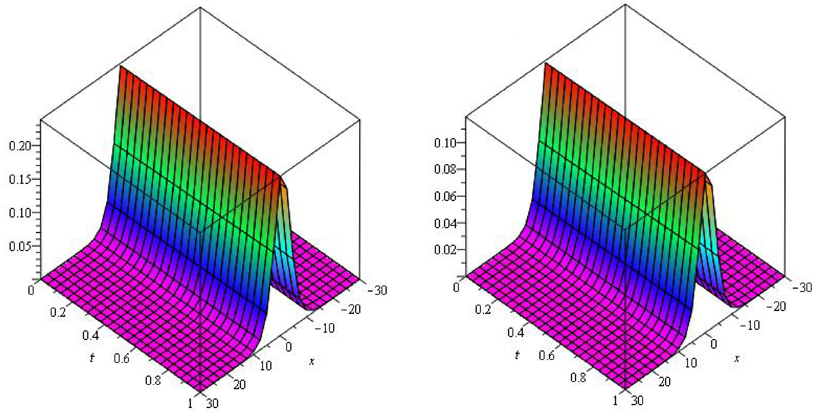
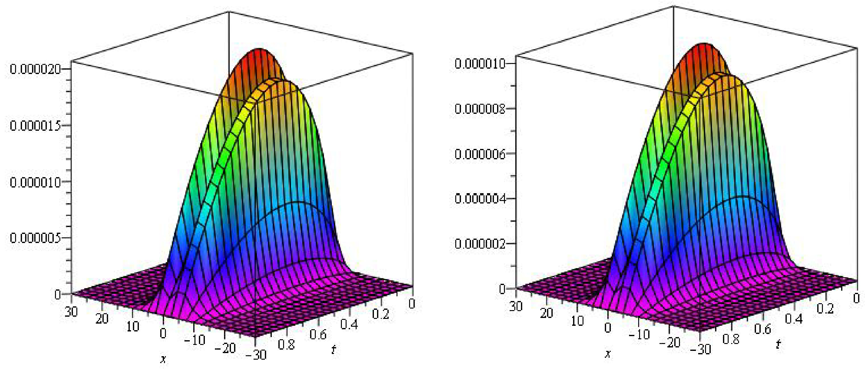
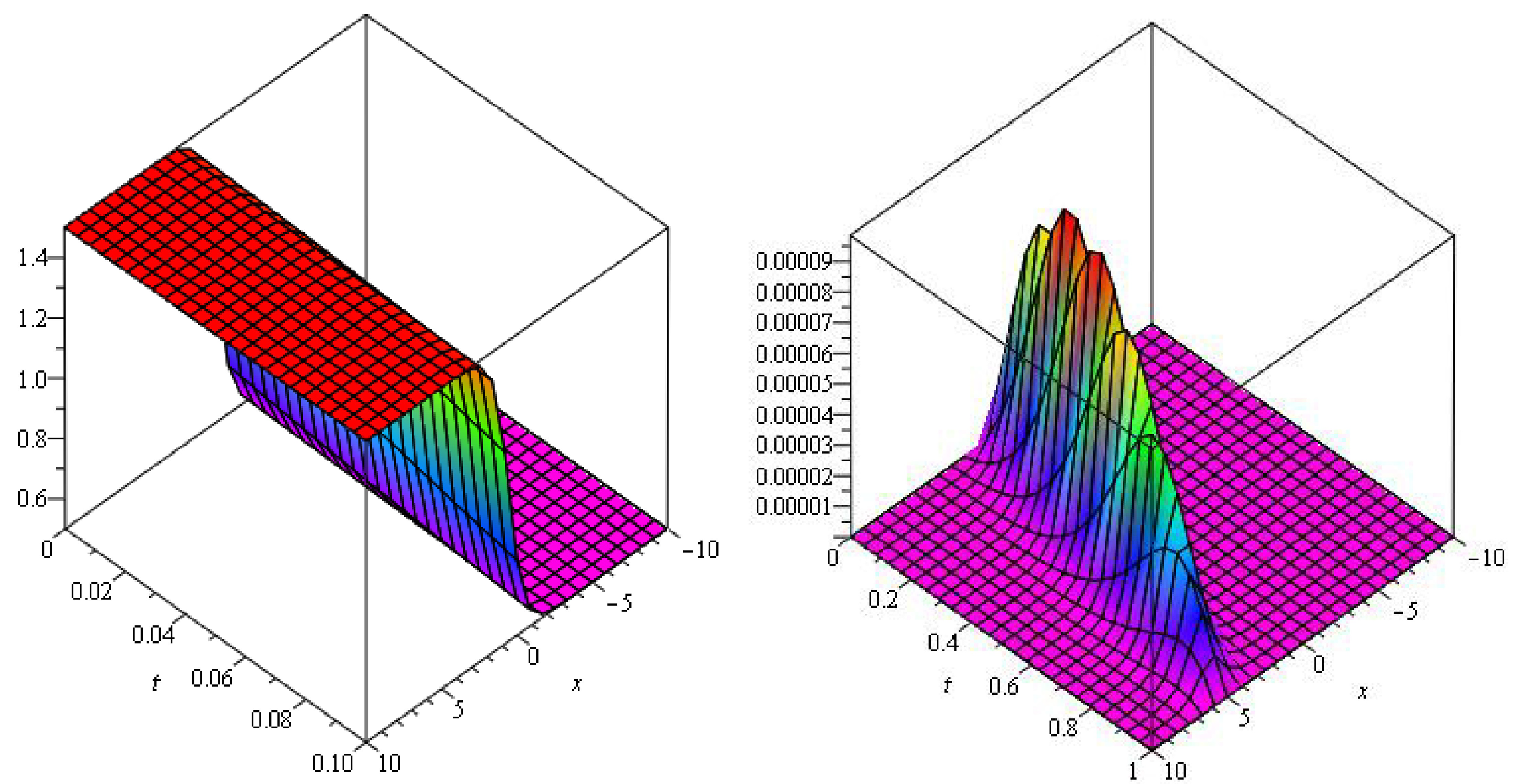
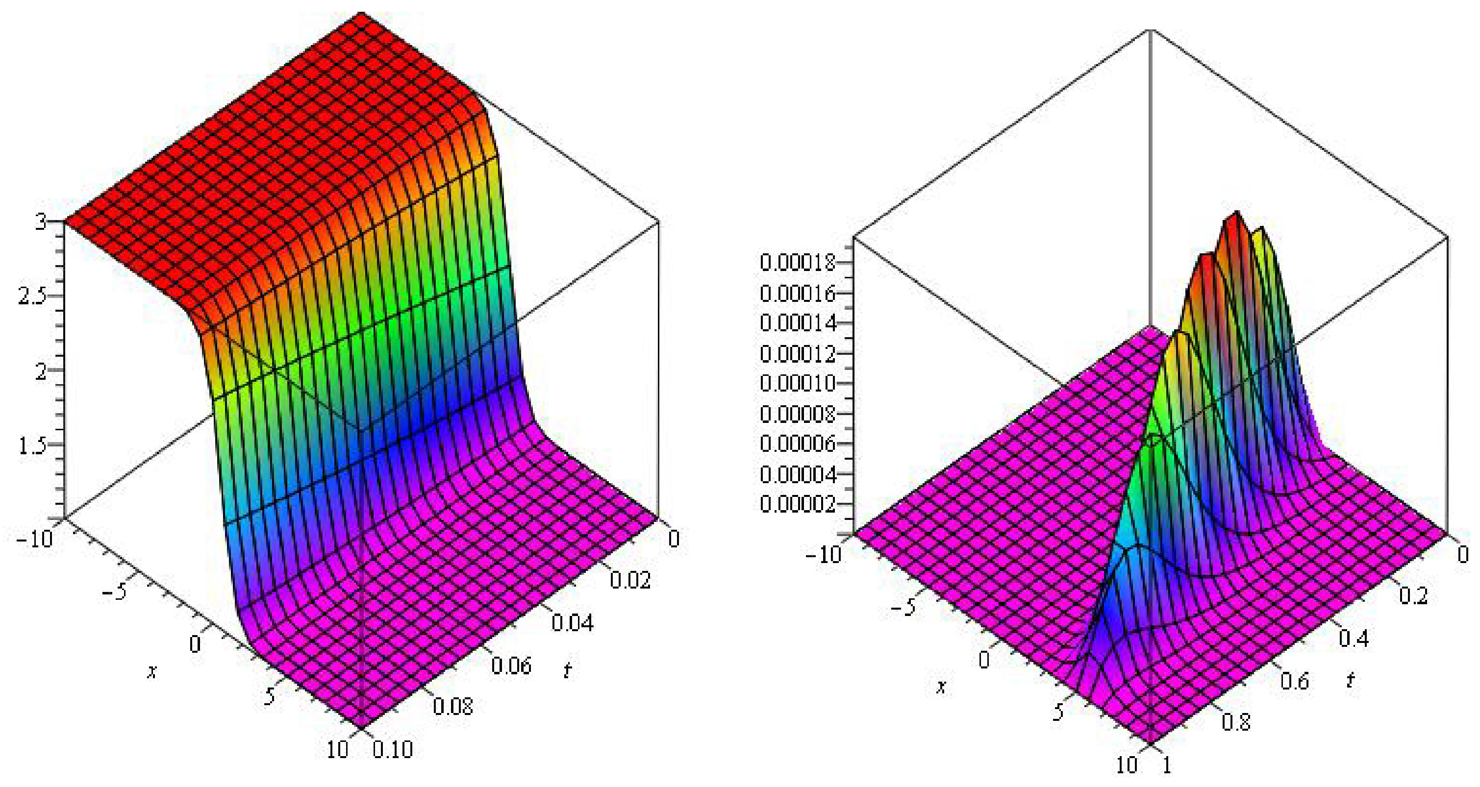
In Figure 1, the analytical solutions of $\mu (\zeta ,\tau )$ and $\nu (\zeta ,\tau )$ are plotted in at $\rho =1$ and the close contact of the actual and NITM solutions is analyzed. In Figure 2, the graphs represents the error plot of analytical solutions at $\rho =1$ of Example 1. The

Table 1. Table of New iterative transform method for different fractional-order values of $\rho$ when $\eta =0.001$ and Absolute Error of example 1.

ITM		$\mathit{\gamma }=0.55$		App. $\mathit{\rho }=1$		Exact		AE
$\mathbf{\zeta }$	$\mathbf{\tau }$	$\mathbf{\mu }$	$\mathbf{\nu }$	$\mathbf{\mu }$	$\mathbf{\nu }$	$\mathbf{\mu }$	$\mathbf{\nu }$	$\mathbf{\mu }$	$\mathbf{\nu }$
−30	0.1	0.02763	0.00378	0.02654	0.00391	0.02741	0.00271	7.3 $\times {10}^{-6}$	4.7 $\times {10}^{-7}$
	0.3	0.02764	0.00375	0.02637	0.00389	0.02769	0.00277	2.2 $\times {10}^{-5}$	1.2 $\times {10}^{-6}$
	0.5	0.02756	0.00373	0.02620	0.00386	0.02757	0.00284	3.4 $\times {10}^{-5}$	2.2 $\times {10}^{-6}$
0	0.1	0.29676	0.04117	0.23657	0.04193	0.29617	0.03106	3.1 $\times {10}^{-5}$	2.2 $\times {10}^{-6}$
	0.3	0.29686	0.04113	0.29378	0.04116	0.29668	0.03114	1.2 $\times {10}^{-4}$	7.8 $\times {10}^{-6}$
	0.5	0.29662	0.04145	0.29839	0.04118	0.29640	0.03131	1.7 $\times {10}^{-4}$	1.5 $\times {10}^{-5}$
30	0.1	0.00370	0.00047	0.00347	0.00049	0.00346	0.00039	1.3 $\times {10}^{-6}$	7.1 $\times {10}^{-8}$
	0.3	0.00346	0.00047	0.00347	0.00049	0.00346	0.00039	3.851 $\times {10}^{-6}$	2.2 $\times {10}^{-7}$
	0.5	0.00347	0.00049	0.00342	0.00049	0.00346	0.00039	5.6 $\times {10}^{-6}$	3.3 $\times {10}^{-7}$

convergence of the fractional solutions can be analyzed to the integer-order solution of the problems.

Example 2.

Consider the fractional-order non-linear dispersive long wave scheme

$$\begin{array}{cc}\hfill & \frac{{\partial }^{\rho }\mu }{\partial {\tau }^{\rho }}=-\frac{\partial \nu }{\partial \zeta }-\frac{1}{2}\frac{\partial {\mu }^2}{\partial \zeta }\hfill \\ \hfill & \frac{{\partial }^{\rho }\nu }{\partial {\tau }^{\rho }}=-\frac{\partial \mu }{\partial \zeta }-\frac{{\partial }^3\mu }{\partial {\zeta }^3}-\frac{\partial \mu \nu }{\partial \zeta },0<\rho <1\hfill \end{array}$$

(26)

with initial condition

$$\mu (\zeta ,0)=a\left[tanh\left(\frac{\eta }{2}+\frac{a\zeta }{2}\right)+1\right],\nu (\zeta ,0)=-1+\frac{1}{2}{a}^{2}sec{h}^2\left(\frac{\eta }{2}+\frac{a\zeta }{2}\right).$$

(27)

While using Elzaki transform of Equation (26), we obtain

$$\begin{array}{cc}\hfill & \frac{1}{{\mathrm{s}}^{\rho }}E\left[\mu (\zeta ,\tau )\right]-\sum _{k=0}^{m-1}{\mu }_{\left(k\right)}(\zeta ,0){\mathrm{s}}^{2-\rho +k}=E\left[-\frac{\partial \nu }{\partial \zeta }-\frac{1}{2}\frac{\partial {\mu }^2}{\partial \zeta }\right],\hfill \\ \hfill & \frac{1}{{\mathrm{s}}^{\rho }}E\left[\nu (\zeta ,\tau )\right]-\sum _{k=0}^{m-1}{\upsilon }_{\left(k\right)}(\zeta ,0){\mathrm{s}}^{2-\rho +k}=E\left[-\frac{\partial \mu }{\partial \zeta }-\frac{{\partial }^3\mu }{\partial {\zeta }^3}-\frac{\partial \mu \nu }{\partial \zeta }\right],\hfill \\ \hfill & \frac{1}{{\mathrm{s}}^{\rho }}E\left[\mu (\zeta ,\tau )\right]={\mu }_{\left(0\right)}(\zeta ,0){\mathrm{s}}^{2-\rho }+E\left[-\frac{\partial \nu }{\partial \zeta }-\frac{1}{2}\frac{\partial {\mu }^2}{\partial \zeta }\right],\hfill \\ \hfill & \frac{1}{{\mathrm{s}}^{\rho }}E\left[\nu (\zeta ,\tau )\right]={\nu }_{\left(0\right)}(\zeta ,0){\mathrm{s}}^{2-\rho }+E\left[-\frac{\partial \mu }{\partial \zeta }-\frac{{\partial }^3\mu }{\partial {\zeta }^3}-\frac{\partial \mu \nu }{\partial \zeta }\right],\hfill \end{array}$$

(28)

$$\begin{array}{cc}\hfill E\left[\mu \right(\zeta ,\tau \left)\right]& ={\mathrm{s}}^2\mu (\zeta ,0)+{\mathrm{s}}^{\rho }E\left[-\frac{\partial \nu }{\partial \zeta }-\frac{1}{2}\frac{\partial {\mu }^2}{\partial \zeta }\right].\hfill \\ \hfill E\left[\nu \right(\zeta ,\tau \left)\right]& ={\mathrm{s}}^2\nu (\zeta ,0)+{\mathrm{s}}^{\rho }E\left[-\frac{\partial \mu }{\partial \zeta }-\frac{{\partial }^3\mu }{\partial {\zeta }^3}-\frac{\partial \mu \nu }{\partial \zeta }\right].\hfill \end{array}$$

(29)

Applying inverse Elzaki transform of Equation (29),

$$\begin{array}{cc}\hfill \mu (\zeta ,\tau )& =E^{-1}\left[{\mathrm{s}}^2\mu (\zeta ,0)\right]+E^{-1}\left[{\mathrm{s}}^{\rho }E\left(-\frac{\partial \nu }{\partial \zeta }-\frac{1}{2}\frac{\partial {\mu }^2}{\partial \zeta }\right)\right].\hfill \\ \hfill \nu (\zeta ,\tau )& =E^{-1}\left[{\mathrm{s}}^2\nu (\zeta ,0)\right]+E^{-1}\left[{\mathrm{s}}^{\rho }E\left(-\frac{\partial \mu }{\partial \zeta }-\frac{{\partial }^3\mu }{\partial {\zeta }^3}-\frac{\partial \mu \nu }{\partial \zeta }\right)\right].\hfill \end{array}$$

(30)

Now, by using the current analytical method, we get

$$\begin{array}{cc}\hfill {\mu }_0(\zeta ,\tau )& =a\left[tanh\left(\frac{\eta }{2}+\frac{a\zeta }{2}\right)+1\right],{\nu }_0(\zeta ,\tau )=-1+\frac{1}{2}{a}^{2}sec{h}^2\left(\frac{\eta }{2}+\frac{a\zeta }{2}\right).\hfill \\ \hfill {\mu }_1(\zeta ,\tau )& =E^{-1}\left[{\mathrm{s}}^{\rho }E\left(-\frac{\partial {\nu }_0}{\partial \zeta }-\frac{1}{2}\frac{\partial {{\mu }_0}^2}{\partial \zeta }\right)\right].\hfill \\ \hfill {\nu }_1(\zeta ,\tau )& =E^{-1}\left[{\mathrm{s}}^{\rho }E\left(-\frac{\partial {\mu }_0}{\partial \zeta }-\frac{{\partial }^3{\mu }_0}{\partial {\zeta }^3}-\frac{\partial {\mu }_0{\nu }_0}{\partial \zeta }\right)\right].\hfill \\ \hfill u_1(\zeta ,\tau )& =-\frac{a^2}{2}sec{h}^2\left(\frac{\eta }{2}+\frac{a\zeta }{2}\right)\frac{{\tau }^{\rho }}{{\Gamma }(\rho +1)},\hfill \\ \hfill {\nu }_1(\zeta ,\tau )& =\frac{a^3}{2}sinh\left(\frac{\eta }{2}+\frac{a\zeta }{2}\right)sec{h}^3\left(\frac{\eta }{2}+\frac{a\zeta }{2}\right)\frac{{\tau }^{\rho }}{{\Gamma }(\rho +1)}.\hfill \\ \hfill {\mu }_2(\zeta ,\tau )& =E^{-1}\left[{\mathrm{s}}^{\rho }E\left(-\frac{\partial {\nu }_1}{\partial \zeta }-\frac{1}{2}\frac{\partial {{\mu }_1}^2}{\partial \zeta }\right)\right].\hfill \\ \hfill {\nu }_2(\zeta ,\tau )& =E^{-1}\left[{\mathrm{s}}^{\rho }E\left(-\frac{\partial {\mu }_1}{\partial \zeta }-\frac{{\partial }^3{\mu }_1}{\partial {\zeta }^3}-\frac{\partial {\mu }_1{\nu }_1}{\partial \zeta }\right)\right].\hfill \\ \hfill {\mu }_2(\zeta ,\tau )& -\frac{a^5}{4}sec{h}^2\left(\frac{\eta }{2}+\frac{a\zeta }{2}\right)\frac{{\tau }^{2\rho }}{{\Gamma }(2\rho +1)}+\frac{3a^5}{4}sin{h}^2\left(\frac{\eta }{2}+\frac{a\zeta }{2}\right)sec{h}^4\left(\frac{\eta }{2}+\frac{a\zeta }{2}\right)\frac{{\tau }^{2\rho }}{{\Gamma }(2\rho +1)}\hfill \\ \hfill & +\frac{a^7}{4}sinh\left(\frac{\eta }{2}+\frac{a\zeta }{2}\right)sec{h}^5\left(\frac{\eta }{2}+\frac{a\zeta }{2}\right)\frac{{\Gamma }(2\rho +1){\tau }^{3\rho }}{{\Gamma }(3\rho +1){\Gamma }{(\rho +1)}^2},\hfill \\ \hfill {\nu }_2(\zeta ,\tau )& =\frac{a^6}{4}[2cos{h}^2\left(\frac{\eta }{2}+\frac{a\zeta }{2}\right)-3]sec{h}^4\left(\frac{\eta }{2}+\frac{a\zeta }{2}\right)\frac{{\tau }^{2\rho }}{{\Gamma }(2\rho +1)}.\hfill \\ \hfill ⋮\\ \hfill {\mu }_n(\zeta ,\tau )& =E^{-1}\left[{\mathrm{s}}^{\rho }E\left(-\frac{\partial {\nu }_{n-1}}{\partial \zeta }-\frac{1}{2}\frac{\partial {\left({\mu }_{n-1}\right)}^2}{\partial \zeta }\right)\right].\hfill \\ \hfill {\nu }_n(\zeta ,\tau )& =E^{-1}\left[{\mathrm{s}}^{\rho }E\left(-\frac{\partial {\mu }_{n-1}}{\partial \zeta }-\frac{{\partial }^3{\mu }_{n-1}}{\partial {\zeta }^3}-\frac{\partial {\mu }_{n-1}{\nu }_{n-1}}{\partial \zeta }\right)\right].n\ge 0.\hfill \end{array}$$

The series form result is given as

$$\begin{array}{c}\hfill \mu (\zeta ,\tau )={\mu }_0(\zeta ,\tau )+{\mu }_1(\zeta ,\tau )+{\mu }_2(\zeta ,\tau )+{\mu }_3(\zeta ,\tau )+\cdots {\mu }_n(\zeta ,\tau )\\ \hfill \nu (\zeta ,\tau )={\nu }_0(\zeta ,\tau )+{\nu }_1(\zeta ,\tau )+{\nu }_2(\zeta ,\tau )+{\nu }_3(\zeta ,\tau )+\cdots {\nu }_n(\zeta ,\tau )\end{array}$$

(31)

$$\begin{array}{c}u(\zeta ,\tau )=a\left[tanh\left(\frac{\eta }{2}+\frac{a\zeta }{2}\right)+1\right]-\frac{a^3}{2}sec{h}^2\left(\frac{\eta }{2}+\frac{a\zeta }{2}\right)\frac{{\tau }^{\rho }}{{\Gamma }(\rho +1)}\hfill \\ -\frac{a^5}{4}sec{h}^2\left(\frac{\eta }{2}+\frac{a\zeta }{2}\right)\frac{{\tau }^{2\rho }}{{\Gamma }(2\rho +1)}+\frac{3a^5}{4}sin{h}^2\left(\frac{\eta }{2}+\frac{a\zeta }{2}\right)sec{h}^4\left(\frac{\eta }{2}+\frac{a\zeta }{2}\right)\frac{{\tau }^{2\rho }}{{\Gamma }(2\rho +1)}\hfill \\ +\frac{a^7}{4}sinh\left(\frac{\eta }{2}+\frac{a\zeta }{2}\right)sec{h}^5\left(\frac{\eta }{2}+\frac{a\zeta }{2}\right)\frac{{\Gamma }(2\rho +1){\tau }^{3\rho }}{{\Gamma }(3\rho +1){\Gamma }{(\rho +1)}^2}+\cdots ,\hfill \\ \nu (\zeta ,\tau )=-1+\frac{1}{2}{a}^{2}sec{h}^2\left(\frac{\eta }{2}+\frac{a\zeta }{2}\right)+\frac{a^4}{2}sinh\left(\frac{\eta }{2}+\frac{a\zeta }{2}\right)sec{h}^3\left(\frac{\eta }{2}+\frac{a\zeta }{2}\right)\frac{{\tau }^{\rho }}{{\Gamma }(\rho +1)}\hfill \\ \frac{a^6}{4}[2cos{h}^2\left(\frac{\eta }{2}+\frac{a\zeta }{2}\right)-3]sec{h}^4\left(\frac{\eta }{2}+\frac{a\zeta }{2}\right)\frac{{\tau }^{2\rho }}{{\Gamma }(2\rho +1)}+\cdots ,\hfill \end{array}$$

For $\rho =1$, the exact results of KdV scheme Equation (26) is given by

$$\begin{array}{cc}\hfill & u(\zeta ,\tau )=a\left[tanh\left(\frac{\eta }{2}+\frac{a\zeta }{2}-\frac{a^2\tau }{2}\right)+1\right],\hfill \\ & v(\zeta ,\tau )=-1+\frac{1}{2}{a}^{2}sec{h}^2\left(\frac{\eta }{2}+\frac{a\zeta }{2}-\frac{a^2\tau }{2}\right).\hfill \end{array}$$

(32)

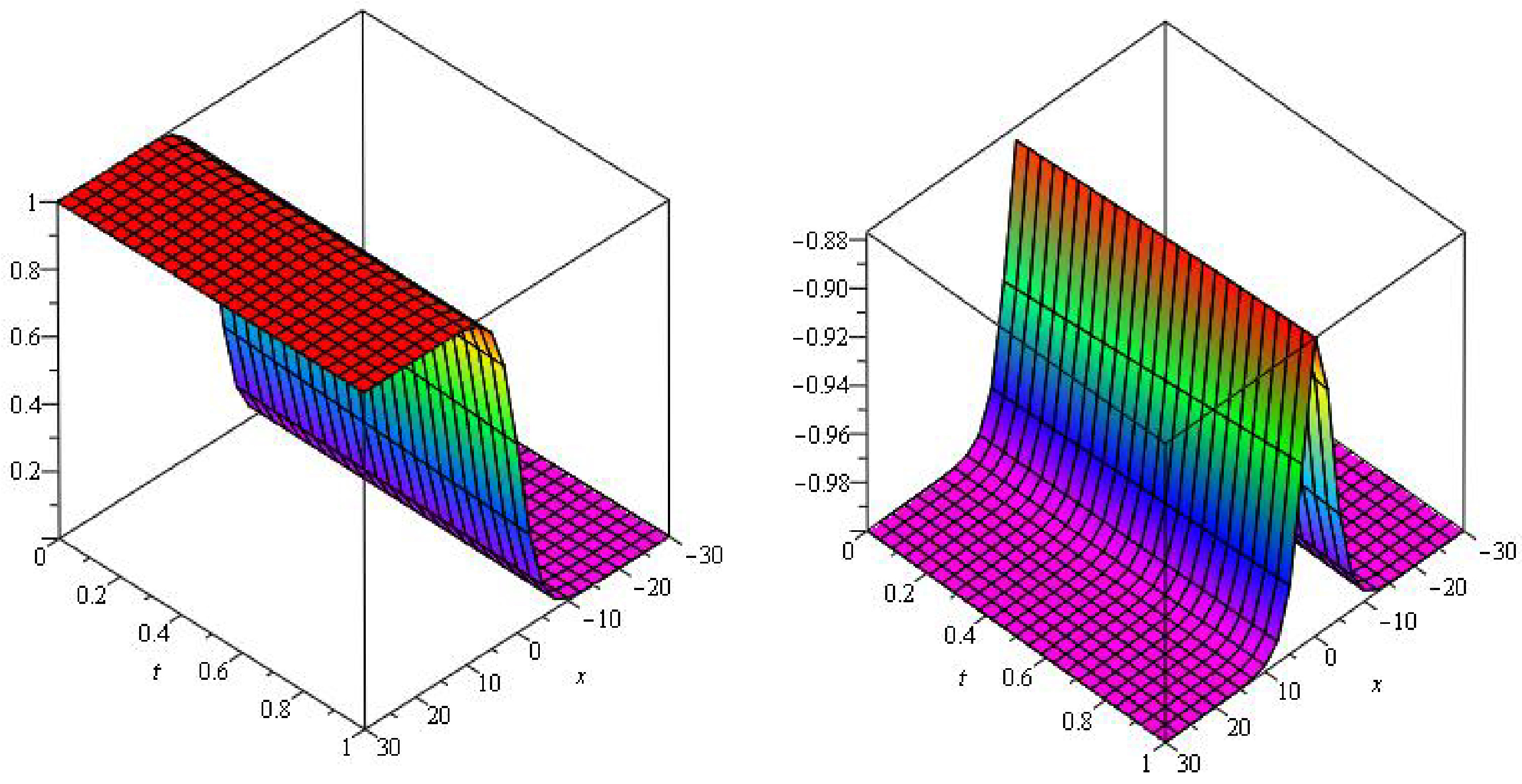
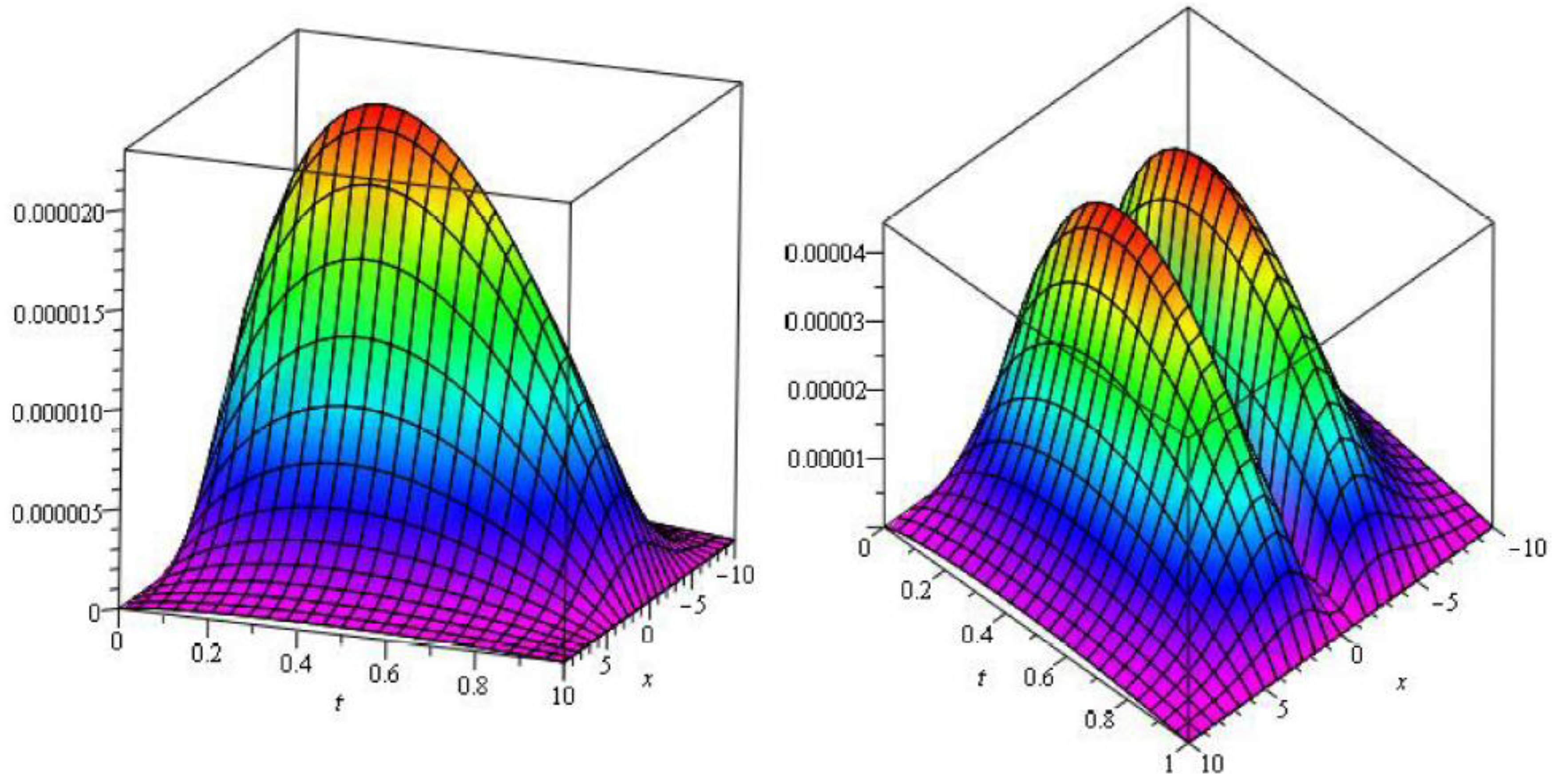
In Figure 3, the analytical solutions of $\mu (\zeta ,\tau )$ and $\nu (\zeta ,\tau )$ are plotted in at $\rho =1$ and the close contact of the actual and NITM solutions is analyzed. In Figure 4, the graphs represents the error plot of analytical solutions at $\alpha =1$ of Example 2.

Example 3.

Consider the non-linear fractional-order new coupled modified KdV system

$$\begin{array}{cc}\hfill \frac{{\partial }^{\rho }\mu }{\partial {\tau }^{\rho }}& =\frac{1}{2}\frac{{\partial }^3\mu }{\partial {\tau }^3}-3{\mu }^2\frac{\partial \mu }{\partial \zeta }+\frac{3}{2}\omega \frac{{\partial }^2\nu }{\partial {\zeta }^2}+3\frac{\partial \nu }{\partial \zeta }\frac{\partial \omega }{\partial \zeta }+\frac{3}{2}\nu \frac{{\partial }^2\omega }{\partial {\zeta }^2}+3\nu \omega \frac{\partial \mu }{\partial \zeta }+3\mu \omega \frac{\partial \nu }{\partial \zeta }+3\mu \nu \frac{\partial \omega }{\partial \zeta },\hfill \\ \hfill \frac{{\partial }^{\rho }\nu }{\partial {\tau }^{\rho }}& =-\frac{{\partial }^3\nu }{\partial {\zeta }^3}-3\frac{\partial \mu }{\partial \zeta }\frac{\partial \nu }{\partial \zeta }-3\nu \frac{{\partial }^2\mu }{\partial {\zeta }^2}-3{\nu }^2\frac{\partial \omega }{\partial \zeta }+6\mu \nu \frac{\partial \mu }{\partial \zeta }+3{\mu }^2\frac{\partial \nu }{\partial \zeta },\hfill \\ \hfill \frac{{\partial }^{\rho }\omega }{\partial {\tau }^{\rho }}& =-\frac{{\partial }^3\omega }{\partial {\zeta }^3}-3\frac{\partial \mu }{\partial \zeta }\frac{\partial \omega }{\partial \zeta }-3\omega \frac{{\partial }^2\mu }{\partial {\zeta }^2}-3{\omega }^2\frac{\partial \nu }{\partial \zeta }+6\mu \omega \frac{\partial \mu }{\partial \zeta }+3{\mu }^2\frac{\partial \omega }{\partial \zeta },\hfill \end{array}$$

(33)

with initial conditions

$$\mu (\zeta ,0)=1+\frac{1}{2}tanh\left(\zeta \right),\nu (\zeta ,0)=\frac{1}{2}-\frac{1}{4}tanh\left(\zeta \right),\omega (\zeta ,0)=2-tanh\left(\zeta \right).$$

(34)

Using Elzaki transform to Equation (33), we get -4.6cm0cm

$$\begin{array}{cc}\hfill \frac{1}{{\mathrm{s}}^{\rho }}E\left[\mu (\zeta ,\tau )\right]-\sum _{k=0}^{m-1}{\mu }_{\left(k\right)}(\zeta ,0){\mathrm{s}}^{2-\rho +k}& =E[\frac{1}{2}\frac{{\partial }^3\mu }{\partial {\tau }^3}-3{\mu }^2\frac{\partial \mu }{\partial \zeta }+\frac{3}{2}\omega \frac{{\partial }^2\nu }{\partial {\zeta }^2}+3\frac{\partial \nu }{\partial \zeta }\frac{\partial \omega }{\partial \zeta }+\frac{3}{2}\nu \frac{{\partial }^2\omega }{\partial {\zeta }^2}\hfill \\ \hfill & +3\nu \omega \frac{\partial \mu }{\partial \zeta }+3\mu \omega \frac{\partial \nu }{\partial \zeta }+3\mu \nu \frac{\partial \omega }{\partial \zeta }],\hfill \\ \hfill \frac{1}{{\mathrm{s}}^{\rho }}E\left[\nu (\zeta ,\tau )\right]-\sum _{k=0}^{m-1}{\nu }_{\left(k\right)}(\zeta ,0){\mathrm{s}}^{2-\rho +k}& =E[-\frac{{\partial }^3\nu }{\partial {\zeta }^3}-3\frac{\partial \mu }{\partial \zeta }\frac{\partial \nu }{\partial \zeta }-3\nu \frac{{\partial }^2\mu }{\partial {\zeta }^2}-3{\nu }^2\frac{\partial \omega }{\partial \zeta }\hfill \\ \hfill & +6\mu \nu \frac{\partial \mu }{\partial \zeta }+3{\mu }^2\frac{\partial \nu }{\partial \zeta }],\hfill \\ \hfill \frac{1}{{\mathrm{s}}^{\rho }}E\left[\omega (\zeta ,\tau )\right]-\sum _{k=0}^{m-1}{\omega }_{\left(k\right)}(\zeta ,0){\mathrm{s}}^{2-\rho +k}& =E[-\frac{{\partial }^3\omega }{\partial {\zeta }^3}-3\frac{\partial \mu }{\partial \zeta }\frac{\partial \omega }{\partial \zeta }-3\omega \frac{{\partial }^2\mu }{\partial {\zeta }^2}-3{\omega }^2\frac{\partial \nu }{\partial \zeta }\hfill \\ \hfill & +6\mu \omega \frac{\partial \mu }{\partial \zeta }+3{\mu }^2\frac{\partial \omega }{\partial \zeta }],\hfill \end{array}$$

(35)

$$\begin{array}{cc}\hfill \frac{1}{{\mathrm{s}}^{\rho }}E\left[\mu (\zeta ,\tau )\right]={\mu }_{\left(0\right)}(\zeta ,0){\mathrm{s}}^{2-\rho }+& E[\frac{1}{2}\frac{{\partial }^3\mu }{\partial {\tau }^3}-3{\mu }^2\frac{\partial \mu }{\partial \zeta }+\frac{3}{2}\omega \frac{{\partial }^2\nu }{\partial {\zeta }^2}+3\frac{\partial \nu }{\partial \zeta }\frac{\partial \omega }{\partial \zeta }+\frac{3}{2}\nu \frac{{\partial }^2\omega }{\partial {\zeta }^2}\hfill \\ \hfill & +3\nu \omega \frac{\partial \mu }{\partial \zeta }+3\mu \omega \frac{\partial \nu }{\partial \zeta }+3\mu \nu \frac{\partial \omega }{\partial \zeta }],\hfill \\ \hfill \frac{1}{{\mathrm{s}}^{\rho }}E\left[\nu (\zeta ,\tau )\right]={\nu }_{\left(0\right)}(\zeta ,0){\mathrm{s}}^{2-\rho }+& E[-\frac{{\partial }^3\nu }{\partial {\zeta }^3}-3\frac{\partial \mu }{\partial \zeta }\frac{\partial \nu }{\partial \zeta }-3\nu \frac{{\partial }^2\mu }{\partial {\zeta }^2}-3{\nu }^2\frac{\partial \omega }{\partial \zeta }\hfill \\ \hfill & +6\mu \nu \frac{\partial \mu }{\partial \zeta }+3{\mu }^2\frac{\partial \nu }{\partial \zeta }],\hfill \\ \hfill \frac{1}{{\mathrm{s}}^{\rho }}E\left[\omega (\zeta ,\tau )\right]={\omega }_{\left(0\right)}(\zeta ,0){\mathrm{s}}^{2-\rho }+& E[-\frac{{\partial }^3\omega }{\partial {\zeta }^3}-3\frac{\partial \mu }{\partial \zeta }\frac{\partial \omega }{\partial \zeta }-3\omega \frac{{\partial }^2\mu }{\partial {\zeta }^2}-3{\omega }^2\frac{\partial \nu }{\partial \zeta }\hfill \\ \hfill & +6\mu \omega \frac{\partial \mu }{\partial \zeta }+3{\mu }^2\frac{\partial \omega }{\partial \zeta }],\hfill \end{array}$$

(36)

$$\begin{array}{cc}\hfill E\left[\mu \right(\zeta ,\tau \left)\right]& ={\mathrm{s}}^2\mu (\zeta ,0)+{\mathrm{s}}^{\rho }E[\frac{1}{2}\frac{{\partial }^3\mu }{\partial {\tau }^3}-3{\mu }^2\frac{\partial \mu }{\partial \zeta }+\frac{3}{2}\omega \frac{{\partial }^2\nu }{\partial {\zeta }^2}+3\frac{\partial \nu }{\partial \zeta }\frac{\partial \omega }{\partial \zeta }+\frac{3}{2}\nu \frac{{\partial }^2\omega }{\partial {\zeta }^2}\hfill \\ \hfill & +3\nu \omega \frac{\partial \mu }{\partial \zeta }+3\mu \omega \frac{\partial \nu }{\partial \zeta }+3\mu \nu \frac{\partial \omega }{\partial \zeta }].\hfill \\ \hfill E\left[\nu \right(\zeta ,\tau \left)\right]& ={\mathrm{s}}^2\nu (\zeta ,0)+{\mathrm{s}}^{\rho }E\left[-\frac{{\partial }^3\nu }{\partial {\zeta }^3}-3\frac{\partial \mu }{\partial \zeta }\frac{\partial \nu }{\partial \zeta }-3\nu \frac{{\partial }^2\mu }{\partial {\zeta }^2}-3{\nu }^2\frac{\partial \omega }{\partial \zeta }+6\mu \nu \frac{\partial \mu }{\partial \zeta }+3{\mu }^2\frac{\partial \nu }{\partial \zeta }\right].\hfill \\ \hfill E\left[\omega \right(\zeta ,\tau \left)\right]& ={\mathrm{s}}^2\omega (\zeta ,0)+{\mathrm{s}}^{\rho }E\left[-\frac{{\partial }^3\omega }{\partial {\zeta }^3}-3\frac{\partial \mu }{\partial \zeta }\frac{\partial \omega }{\partial \zeta }-3\omega \frac{{\partial }^2\mu }{\partial {\zeta }^2}-3{\omega }^2\frac{\partial \nu }{\partial \zeta }+6\mu \omega \frac{\partial \mu }{\partial \zeta }+3{\mu }^2\frac{\partial \omega }{\partial \zeta }\right].\hfill \end{array}$$

(37)

Applying inverse Elzaki transform of Equation (37),

$$\begin{array}{cc}\hfill \mu (\zeta ,\tau )& =E^{-1}\left[{\mathrm{s}}^2\mu (\zeta ,0)\right]+E^{-1}\left[{\mathrm{s}}^{\rho }E\right(\frac{1}{2}\frac{{\partial }^3\mu }{\partial {\tau }^3}-3{\mu }^2\frac{\partial \mu }{\partial \zeta }+\frac{3}{2}\omega \frac{{\partial }^2\nu }{\partial {\zeta }^2}+3\frac{\partial \nu }{\partial \zeta }\frac{\partial \omega }{\partial \zeta }+\frac{3}{2}\nu \frac{{\partial }^2\omega }{\partial {\zeta }^2}\hfill \\ \hfill & +3\nu \omega \frac{\partial \mu }{\partial \zeta }+3\mu \omega \frac{\partial \nu }{\partial \zeta }+3\mu \nu \frac{\partial \omega }{\partial \zeta }\left)\right].\hfill \\ \hfill \nu (\zeta ,\tau )& =E^{-1}\left[{\mathrm{s}}^2\nu (\zeta ,0)\right]+E^{-1}\left[{\mathrm{s}}^{\rho }E\right(-\frac{{\partial }^3\nu }{\partial {\zeta }^3}-3\frac{\partial \mu }{\partial \zeta }\frac{\partial \nu }{\partial \zeta }-3\nu \frac{{\partial }^2\mu }{\partial {\zeta }^2}-3{\nu }^2\frac{\partial \omega }{\partial \zeta }\hfill \\ \hfill & +6\mu \nu \frac{\partial \mu }{\partial \zeta }+3{\mu }^2\frac{\partial \nu }{\partial \zeta }\left)\right].\hfill \\ \hfill \omega (\zeta ,\tau )& =E^{-1}\left[{\mathrm{s}}^2\omega (\zeta ,0)\right]+E^{-1}\left[{\mathrm{s}}^{\rho }E\right(-\frac{{\partial }^3\omega }{\partial {\zeta }^3}-3\frac{\partial \mu }{\partial \zeta }\frac{\partial \omega }{\partial \zeta }-3\omega \frac{{\partial }^2\mu }{\partial {\zeta }^2}-3{\omega }^2\frac{\partial \nu }{\partial \zeta }\hfill \\ \hfill & +6\mu \omega \frac{\partial \mu }{\partial \zeta }+3{\mu }^2\frac{\partial \omega }{\partial \zeta }\left)\right].\hfill \end{array}$$

(38)

Now, by using the suggested analytical method, we get

$$\begin{array}{cc}\hfill {\mu }_0(\zeta ,\tau )& =1+\frac{1}{2}tanh\left(\zeta \right),{\nu }_0(\zeta ,\tau )=\frac{1}{2}-\frac{1}{4}tanh\left(\zeta \right),{\omega }_0(\zeta ,\tau )=2-tanh\left(\zeta \right).\hfill \\ \hfill {\mu }_1(\zeta ,\tau )& =E^{-1}\left[{\mathrm{s}}^{\rho }E\right(\frac{1}{2}\frac{{\partial }^3{\mu }_0}{\partial {\tau }^3}-3{\mu }_0^2\frac{\partial {\mu }_0}{\partial \zeta }+\frac{3}{2}{\omega }_0\frac{{\partial }^2{\nu }_0}{\partial {\zeta }^2}+3\frac{\partial {\nu }_0}{\partial \zeta }\frac{\partial {\omega }_0}{\partial \zeta }+\frac{3}{2}{\nu }_0\frac{{\partial }^2{\omega }_0}{\partial {\zeta }^2}\hfill \\ \hfill & +3{\nu }_0{\omega }_0\frac{\partial {\mu }_0}{\partial \zeta }+3{\mu }_0{\omega }_0\frac{\partial {\nu }_0}{\partial \zeta }+3{\mu }_0{\nu }_0\frac{\partial {\omega }_0}{\partial \zeta }\left)\right].\hfill \\ \hfill {\nu }_1(\zeta ,\tau )& =E^{-1}\left[{\mathrm{s}}^{\rho }E\right(-\frac{{\partial }^3{\nu }_0}{\partial {\zeta }^3}-3\frac{\partial {\mu }_0}{\partial \zeta }\frac{\partial {\nu }_0}{\partial \zeta }-3{\nu }_0\frac{{\partial }^2{\mu }_0}{\partial {\zeta }^2}-3{\nu }_0^2\frac{\partial {\omega }_0}{\partial \zeta }\hfill \\ \hfill & +6{\mu }_0{\nu }_0\frac{\partial {\mu }_0}{\partial \zeta }+3{\mu }_0^2\frac{\partial {\nu }_0}{\partial \zeta }\left)\right].\hfill \\ \hfill {\omega }_1(\zeta ,\tau )& =E^{-1}\left[{\mathrm{s}}^{\rho }E\right(-\frac{{\partial }^3{\omega }_0}{\partial {\zeta }^3}-3\frac{\partial {\mu }_0}{\partial \zeta }\frac{\partial {\omega }_0}{\partial \zeta }-3{\omega }_0\frac{{\partial }^2{\mu }_0}{\partial {\zeta }^2}-3{\omega }_0^2\frac{\partial {\nu }_0}{\partial \zeta }\hfill \\ \hfill & +6{\mu }_0{\omega }_0\frac{\partial {\mu }_0}{\partial \zeta }+3{\mu }_0^2\frac{\partial {\omega }_0}{\partial \zeta }\left)\right].\hfill \end{array}$$

$$\begin{array}{cc}\hfill {\mu }_1(\zeta ,\tau )& =\frac{11}{2}sec{h}^2\left(\zeta \right)\frac{{\eta }^{\rho }}{{\Gamma }(\rho +1)},{\nu }_1(\zeta ,\tau )=-\frac{11}{8}sec{h}^2\left(\zeta \right)\frac{{\eta }^{\rho }}{{\Gamma }(\rho +1)},\hfill \\ \hfill {\omega }_1(\zeta ,\tau )& =-\frac{11}{2}sec{h}^2\left(\zeta \right)\frac{{\eta }^{\rho }}{{\Gamma }(\rho +1)}.\hfill \end{array}$$

$$\begin{array}{cc}\hfill {\mu }_2(\zeta ,\tau )& =E^{-1}\left[{\mathrm{s}}^{\rho }E\right(\frac{1}{2}\frac{{\partial }^3{\mu }_1}{\partial {\tau }^3}-3{\mu }_1^2\frac{\partial {\mu }_1}{\partial \zeta }+\frac{3}{2}{\omega }_1\frac{{\partial }^2{\nu }_1}{\partial {\zeta }^2}+3\frac{\partial {\nu }_1}{\partial \zeta }\frac{\partial {\omega }_1}{\partial \zeta }+\frac{3}{2}{\nu }_1\frac{{\partial }^2{\omega }_1}{\partial {\zeta }^2}\hfill \\ \hfill & +3{\nu }_1{\omega }_1\frac{\partial {\mu }_1}{\partial \zeta }+3{\mu }_1{\omega }_1\frac{\partial {\nu }_1}{\partial \zeta }+3{\mu }_1{\nu }_1\frac{\partial {\omega }_1}{\partial \zeta }\left)\right].\hfill \\ \hfill {\nu }_2(\zeta ,\tau )& =E^{-1}\left[{\mathrm{s}}^{\rho }E\left(-\frac{{\partial }^3{\nu }_1}{\partial {\zeta }^3}-3\frac{\partial {\mu }_1}{\partial \zeta }\frac{\partial {\nu }_1}{\partial \zeta }-3{\nu }_1\frac{{\partial }^2{\mu }_1}{\partial {\zeta }^2}-3{\nu }_1^2\frac{\partial {\omega }_1}{\partial \zeta }+6{\mu }_1{\nu }_1\frac{\partial {\mu }_1}{\partial \zeta }+3{\mu }_1^2\frac{\partial {\nu }_1}{\partial \zeta }\right)\right].\hfill \\ \hfill {\omega }_2(\zeta ,\tau )& =E^{-1}\left[{\mathrm{s}}^{\rho }E\left(-\frac{{\partial }^3{\omega }_1}{\partial {\zeta }^3}-3\frac{\partial {\mu }_1}{\partial \zeta }\frac{\partial {\omega }_1}{\partial \zeta }-3{\omega }_1\frac{{\partial }^2{\mu }_1}{\partial {\zeta }^2}-3{\omega }_1^2\frac{\partial {\nu }_1}{\partial \zeta }+6{\mu }_1{\omega }_1\frac{\partial {\mu }_1}{\partial \zeta }+3{\mu }_1^2\frac{\partial {\omega }_1}{\partial \zeta }\right)\right].\hfill \end{array}$$

$$\begin{array}{cc}\hfill {\mu }_2(\zeta ,\tau )& =-\frac{121}{8}tanh\left(\zeta \right)sec{h}^2\left(\zeta \right)\frac{{\eta }^{2\rho }}{{\Gamma }(2\rho +1)},{\nu }_2(\zeta ,\tau )=\frac{121}{8}tanh\left(\zeta \right)sec{h}^2\left(\zeta \right)\frac{{\eta }^{2\rho }}{{\Gamma }(2\rho +1)},\hfill \\ \hfill {\omega }_2(\zeta ,\tau )& =\frac{121}{4}tanh\left(\zeta \right)sec{h}^2\left(\zeta \right)\frac{{\eta }^{2\rho }}{{\Gamma }(2\rho +1)}.\hfill \end{array}$$

$$\begin{array}{cc}\hfill {\mu }_3(\zeta ,\tau )& =\frac{1331}{48}(cosh\left(2\zeta \right)-2)sec{h}^4\left(\zeta \right)\frac{{\eta }^{3\rho }}{{\Gamma }(3\rho +1)},\hfill \\ \hfill {\nu }_3(\zeta ,\tau )& =-\frac{1331}{96}(cosh\left(2\zeta \right)-2)sec{h}^4\left(\zeta \right)\frac{{\eta }^{3\rho }}{{\Gamma }(3\rho +1)},\hfill \\ \hfill {\omega }_3(\zeta ,\tau )& =-\frac{1331}{24}(cosh\left(2\zeta \right)-2)sec{h}^4\left(\zeta \right)\frac{{\eta }^{3\rho }}{{\Gamma }(3\rho +1)}.\hfill \\ \hfill ⋮\\ \hfill {\mu }_n(\zeta ,\tau )=& E^{-1}\left[{\mathrm{s}}^{\rho }E\right(\frac{1}{2}\frac{{\partial }^3{\mu }_{n-1}}{\partial {\tau }^3}-3{\mu }_{n-1}^2\frac{\partial {\mu }_{n-1}}{\partial \zeta }+\frac{3}{2}{\omega }_{n-1}\frac{{\partial }^2{\nu }_{n-1}}{\partial {\zeta }^2}+3\frac{\partial {\nu }_{n-1}}{\partial \zeta }\frac{\partial {\omega }_{n-1}}{\partial \zeta }\hfill \\ \hfill & +\frac{3}{2}{\nu }_{n-1}\frac{{\partial }^2{\omega }_{n-1}}{\partial {\zeta }^2}+3{\nu }_{n-1}{\omega }_{n-1}\frac{\partial {\mu }_{n-1}}{\partial \zeta }+3{\mu }_{n-1}{\omega }_{n-1}\frac{\partial {\nu }_{n-1}}{\partial \zeta }+3{\mu }_{n-1}{\nu }_{n-1}\frac{\partial {\omega }_{n-1}}{\partial \zeta }\left)\right].\hfill \\ \hfill {\nu }_n(\zeta ,\tau )=& E^{-1}\left[{\mathrm{s}}^{\rho }E\right(-\frac{{\partial }^3{\nu }_{n-1}}{\partial {\zeta }^3}-3\frac{\partial {\mu }_{n-1}}{\partial \zeta }\frac{\partial {\nu }_{n-1}}{\partial \zeta }-3{\nu }_{n-1}\frac{{\partial }^2{\mu }_{n-1}}{\partial {\zeta }^2}-3{\nu }_{n-1}^2\frac{\partial {\omega }_{n-1}}{\partial \zeta }\hfill \\ \hfill & +6{\mu }_{n-1}{\nu }_{n-1}\frac{\partial {\mu }_{n-1}}{\partial \zeta }+3{\mu }_{n-1}^2\frac{\partial {\nu }_{n-1}}{\partial \zeta }\left)\right].\hfill \\ \hfill {\omega }_n(\zeta ,\tau )=& E^{-1}\left[{\mathrm{s}}^{\rho }E\right(-\frac{{\partial }^3{\omega }_{n-1}}{\partial {\zeta }^3}-3\frac{\partial {\mu }_{n-1}}{\partial \zeta }\frac{\partial {\omega }_{n-1}}{\partial \zeta }-3{\omega }_{n-1}\frac{{\partial }^2{\mu }_{n-1}}{\partial {\zeta }^2}\hfill \\ \hfill & -3{\omega }_{n-1}^2\frac{\partial {\nu }_{n-1}}{\partial \zeta }+6{\mu }_{n-1}{\omega }_{n-1}\frac{\partial {\mu }_{n-1}}{\partial \zeta }+3{\mu }_{n-1}^2\frac{\partial {\omega }_{n-1}}{\partial \zeta }\left)\right].\hfill \end{array}$$

The series form result is given as

$$\begin{array}{cc}\hfill \mu (\zeta ,\tau )& ={\mu }_0(\zeta ,\tau )+{\mu }_1(\zeta ,\tau )+{\mu }_2(\zeta ,\tau )+{\mu }_3(\zeta ,\tau )+\cdots {\mu }_n(\zeta ,\tau )\hfill \\ \hfill \nu (\zeta ,\tau )& ={\nu }_0(\zeta ,\tau )+{\nu }_1(\zeta ,\tau )+{\nu }_2(\zeta ,\tau )+{\nu }_3(\zeta ,\tau )+\cdots {\nu }_n(\zeta ,\tau )\hfill \\ \hfill \omega (\zeta ,\tau )& ={\omega }_0(\zeta ,\tau )+{\omega }_1(\zeta ,\tau )+{\omega }_2(\zeta ,\tau )+{\omega }_3(\zeta ,\tau )+\cdots {\omega }_n(\zeta ,\tau )\hfill \end{array}$$

(39)

$$\begin{array}{cc}\hfill \mu (\zeta ,\tau )=& 1+\frac{1}{2}tanh\left(\zeta \right)+\frac{11}{2}sec{h}^2\left(\zeta \right)\frac{{\eta }^{\rho }}{{\Gamma }(\rho +1)}-\frac{121}{8}tanh\left(\zeta \right)sec{h}^2\left(\zeta \right)\frac{{\eta }^{2\rho }}{{\Gamma }(2\rho +1)}\hfill \\ \hfill & +\frac{1331}{48}(cosh\left(2\zeta \right)-2)sec{h}^4\left(\zeta \right)\frac{{\eta }^{3\rho }}{{\Gamma }(3\rho +1)}+\cdots .\hfill \end{array}$$

$$\begin{array}{cc}\hfill \nu (\zeta ,\tau )=& \frac{1}{2}-\frac{1}{4}tanh\left(\zeta \right)-\frac{11}{8}sec{h}^2\left(\zeta \right)\frac{{\eta }^{\rho }}{{\Gamma }(\rho +1)}+\frac{121}{8}tanh\left(\zeta \right)sec{h}^2\left(\zeta \right)\frac{{\eta }^{2\rho }}{{\Gamma }(2\rho +1)}\hfill \\ \hfill & -\frac{1331}{96}(cosh\left(2\zeta \right)-2)sec{h}^4\left(\zeta \right)\frac{{\eta }^{3\rho }}{{\Gamma }(3\rho +1)}+\cdots .\hfill \end{array}$$

$$\begin{array}{cc}\hfill \omega (\zeta ,\tau )=& 2-tanh\left(\zeta \right)-\frac{11}{2}sec{h}^2\left(\zeta \right)\frac{{\eta }^{\rho }}{{\Gamma }(\rho +1)}+\frac{121}{4}tanh\left(\zeta \right)sec{h}^2\left(\zeta \right)\frac{{\eta }^{2\rho }}{{\Gamma }(2\rho +1)}\hfill \\ \hfill & -\frac{1331}{24}(cosh\left(2\zeta \right)-2)sec{h}^4\left(\zeta \right)\frac{{\eta }^{3\rho }}{{\Gamma }(3\rho +1)}+\cdots .\hfill \end{array}$$

The exact result of Equation (33) is

$$\begin{array}{cc}\hfill \mu (\zeta ,\tau )& =1+\frac{1}{2}tanh(\zeta -\frac{11}{2}\eta ),\nu (\zeta ,\tau )=\frac{1}{2}-\frac{1}{4}tanh(\zeta -\frac{11}{2}\eta ),\hfill \\ \hfill \omega (\zeta ,\tau )& =2-tanh(\zeta -\frac{11}{2}\eta ).\hfill \end{array}$$

(40)

In Figure 5, Figure 6 and Figure 7 the analytical solutions of $\mu (\zeta ,\tau )$, $\nu (\zeta ,\tau )$ amd $\omega (\zeta ,\tau )$ solutions are approximate and error at $\rho =1$ of Example 3.

5. Conclusions

In this paper, we have used a combined form of the Iterative method and Elzaki transform method to obtain a numerical solution to the coupled KdV system of equations. It is predicted that the achieved results presented in this article will be useful for further analysis of the complicated non-linear physical problems. The calculations of this technique are very straightforward and simple. Thus, we deduce that this technique can be implemented to solve several schemes of non-linear fractional-order partial differential equations.

References

- Jafari, H.; Jassim, H.; Baleanu, D.; Chu, Y. On the Approximate Solutions for a System of Coupled Korteweg De Vries Equations with Local Fractional Derivative. Fractals 2021. [Google Scholar] [CrossRef]
- Rizvi, S.T.R.; Seadawy, A.R.; Ashraf, F.; Younis, M.; Iqbal, H.; Baleanu, D. Lump and Interaction solutions of a geophysical Korteweg-de Vries equation. Results Phys. 2020, 19, 103661. [Google Scholar] [CrossRef]
- Park, C.; Nuruddeen, R.I.; Ali, K.K.; Muhammad, L.; Osman, M.S.; Baleanu, D. Novel hyperbolic and exponential ansatz methods to the fractional fifth-order Korteweg-de Vries equations. Adv. Differ. Equ. 2020, 1–12. [Google Scholar] [CrossRef]
- Cheemaa, N.; Seadawy, A.R.; Sugati, T.G.; Baleanu, D. Study of the dynamical nonlinear modified Korteweg-de Vries equation arising in plasma physics and its analytical wave solutions. Results Phys. 2020, 19, 103480. [Google Scholar] [CrossRef]
- Kumar, S.; Kumar, A.; Abbas, S.; Al Qurashi, M.; Baleanu, D. A modified analytical approach with existence and uniqueness for fractional Cauchy reaction-diffusion equations. Adv. Differ. Equ. 2020, 1–18. [Google Scholar] [CrossRef]
- Matinfar, M.; Eslami, M.; Kordy, M. The functional variable method for solving the fractional Korteweg-de Vries equations and the coupled Korteweg-de Vries equations. Pramana 2015, 85, 583–592. [Google Scholar] [CrossRef]
- Bekir, A.; Guner, O. Analytical approach for the space-time nonlinear partial differential fractional equation. Int. J. Nonlinear Sci. Numer. Simul. 2014, 15, 463–470. [Google Scholar] [CrossRef]
- Vázquez, L.; Jafari, H. Fractional calculus: Theory and numerical methods. Open Phys. 2013, 11. [Google Scholar] [CrossRef]
- Wu, Y.; Geng, X.; Hu, X.; Zhu, S. A generalized Hirota-Satsuma coupled Korteweg-de Vries equation and Miura transformations. Phys. Lett. A 1999, 255, 259–264. [Google Scholar] [CrossRef]
- Abazari, R.; Abazari, M. Numerical simulation of generalized Hirota-Satsuma coupled KdV equation by RDTM and comparison with DTM. Commun. Nonlinear Sci. Numer. Simul. 2012, 17, 619–629. [Google Scholar] [CrossRef]
- Ganji, D.D.; Rafei, M. Solitary wave solutions for a generalized Hirota-Satsuma coupled KdV equation by homotopy perturbation method. Phys. Lett. A 2006, 356, 131–137. [Google Scholar] [CrossRef]
- Akinyemi, L.; Huseen, S.N. A powerful approach to study the new modified coupled Korteweg-de Vries system. Math. Comput. Simul. 2020, 177, 556–567. [Google Scholar] [CrossRef]
- Chen, C.K.; Ho, S.H. Solving partial differential equations by two-dimensional differential transform method. Appl. Math. Comput. 1999, 106, 171–179. [Google Scholar]
- Gao, Y.T.; Tian, B. Ion-acoustic shocks in space and laboratory dusty plasmas: Two dimensional and non-traveling-wave observable effects. Phys. Plasmas 2001, 8, 3146–3149. [Google Scholar] [CrossRef]
- Osborne, A. The inverse scattering transform: Tools for the nonlinear fourier analysis and filtering of ocean surface waves. Chaos Solitons Fractals 1995, 5, 2623–2637. [Google Scholar] [CrossRef]
- Ostrovsky, L.; Yu, A. Stepanyants, Do internal solutions exist in the ocean. Rev. Geophys. 1989, 27, 293–310. [Google Scholar] [CrossRef]
- Maturi, D. Homotopy Perturbation Method for the Generalized Hirota-Satsuma Coupled KdV Equation. Appl. Math. 2012, 3, 1983–1989. [Google Scholar] [CrossRef] [Green Version]
- Wang, M.; Zhou, Y.; Li, Z. Application of a homogeneous balance method to exact solutions of non-linear equations in mathematical physics. Phys. Lett. A 1996, 216, 67–75. [Google Scholar] [CrossRef]
- Gokdogan, A.; Yildirim, A.; Merdan, M. Solving coupled-KdV equations by differential transformation method. World Appl. Sci. J. 2012, 19, 1823–1828. [Google Scholar]
- Jafari, H.; Firoozjaee, M.A. Homotopy analysis method for solving KdV equations. Surv. Math. Appl. 2010, 5, 89–98. [Google Scholar]
- Lu, D.; Suleman, M.; Ramzan, M.; Ul Rahman, J. Numerical solutions of coupled nonlinear fractional KdV equations using He’s fractional calculus. Int. J. Mod. Phys. B 2021, 35, 2150023. [Google Scholar] [CrossRef]
- Mohamed, M.A.; Torky, M.S. Numerical solution of non-linear system of partial differential equations by the Laplace decomposition method and the Pade approximation. Am. J. Comput. Math. 2013, 3, 175. [Google Scholar] [CrossRef] [Green Version]
- Seadawy, A.R.; El-Rashidy, K. Water wave solutions of the coupled system Zakharov-Kuznetsov and generalized coupled KdV equations. Sci. World J. 2014, 1–6. [Google Scholar] [CrossRef] [PubMed] [Green Version]
- Fan, E. Using symbolic computation to exactly solve a new coupled MKdV system. Phys. Lett. A 2002, 299, 46–48. [Google Scholar] [CrossRef]
- Inc, M.; Cavlak, E. On numerical solutions of a new coupled MKdV system by using the Adomian decomposition method and He’s variational iteration method. Phys. Scr. 2008, 78, 1–7. [Google Scholar] [CrossRef]
- Ghoreishi, M.; Ismail, A.I.; Rashid, A. The solution of coupled modifed KdV system by the homotopy analysis method. TWMS J. Pure Appl. Math. 2012, 3, 122–134. [Google Scholar]
- Daftardar-Gejji, V.; Jafari, H. An iterative method for solving nonlinear functional equations. J. Math. Anal. Appl. 2006, 316, 753–763. [Google Scholar] [CrossRef] [Green Version]
- Jafari, H.; Nazari, M.; Baleanu, D.; Khalique, C.M. A new approach for solving a system of fractional partial differential equations. Comput. Math. Appl. 2013, 66, 838–843. [Google Scholar] [CrossRef]
- Yan, L. Numerical solutions of fractional Fokker-Planck equations using iterative Laplace transform method. Abstr. Appl. Anal. 2013, 2013, 465160. [Google Scholar] [CrossRef]
- Prakash, A.; Kumar, M.; Baleanu, D. A new iterative technique for a fractional model of nonlinear Zakharov-Kuznetsov equations via Sumudu transform. Appl. Math. Comput. 2018, 334, 30–40. [Google Scholar] [CrossRef]
- Ramadan, M.A.; Al-luhaibi, M.S. New iterative method for solving the fornberg-whitham equation and comparison with homotopy perturbation transform method. J. Adv. Math. Comput. Sci. 2014, 4, 1213–1227. [Google Scholar] [CrossRef]
- Alderremy, A.A.; Elzaki, T.M.; Chamekh, M. New transform iterative method for solving some Klein-Gordon equations. Results Phys. 2018, 10, 655–659. [Google Scholar] [CrossRef]
- Elzaki, T.M. On the connections between Laplace and Elzaki transforms. Adv. Theor. Appl. Math. 2011, 6, 1–11. [Google Scholar]
- Elzaki, T.M. On The New Integral Transform “Elzaki Transform” Fundamental Properties Investigations and Applications. Glob. J. Math. Sci. Theory Pract. 2012, 4, 1–13. [Google Scholar]
Figure 1.
Graphs of and at and of example 1.
Figure 2.
Error graphs of and at and of example 1.
Figure 3.
Graphs of and at of example 2.
Figure 4.
Error graphs of and at of example 2.
Figure 5.
Graphs of and error plot at of example 3.
Figure 6.
Figure 7.