
Deep Learning for Wave Energy Converter Modeling Using Long Short-Term Memory


1
Department of Mechanical Engineering, K. N. Toosi University of Technology, Tehran 1999143344, Iran
2
Faculty of Civil Engineering, Technische Universität Dresden, 01069 Dresden, Germany
3
John von Neumann Faculty of Informatics, Obuda University, 1034 Budapest, Hungary
4
School of the Built Environment, Oxford Brookes University, Oxford OX3 0BP, UK
*
Author to whom correspondence should be addressed.
Mathematics 2021, 9(8), 871; https://doi.org/10.3390/math9080871
Submission received: 28 March 2021
/
Revised: 10 April 2021
/
Accepted: 12 April 2021
/
Published: 15 April 2021
Abstract
:Accurate forecasts of ocean waves energy can not only reduce costs for investment, but it is also essential for the management and operation of electrical power. This paper presents an innovative approach based on long short-term memory (LSTM) to predict the power generation of an economical wave energy converter named “Searaser”. The data for analysis is provided by collecting the experimental data from another study and the exerted data from a numerical simulation of Searaser. The simulation is performed with Flow-3D software, which has high capability in analyzing fluid–solid interactions. The lack of relation between wind speed and output power in previous studies needs to be investigated in this field. Therefore, in this study, wind speed and output power are related with an LSTM method. Moreover, it can be inferred that the LSTM network is able to predict power in terms of height more accurately and faster than the numerical solution in a field of predicting. The network output figures show a great agreement, and the root mean square is 0.49 in the mean value related to the accuracy of the LSTM method. Furthermore, the mathematical relation between the generated power and wave height was introduced by curve fitting of the power function to the result of the LSTM method.
1. Introduction
Fossil fuels are still the most essential source of energy in the world [1]. Such non-renewable energy sources significantly contribute to environmental pollution and climate change [2]. Thus, finding alternative energy resources with less carbon footprint is of significant importance. In particular, recently developing non-petroleum-based energy resources has increased tremendously. Among the different sources of renewable energies, solar, wind, tidal and geothermal energies are the most well-known ones [3]. Ocean wave energy has the second largest potential among all ocean renewable energy sources [4].
Absorbing wave energy and transforming it into electricity implies wave energy converters (WECs) that use the motion of ocean surface waves to convert ocean wave energy into electricity. In general, there are different types of WEC systems [5,6]. Due to the important role of WECs in producing electricity from ocean waves, the precise forecast can not only reduce costs for investment but also be essential for the management and operation of electrical power. Due to this fact, investors around the world need information about predicting the potential for power generation by WEC systems [7]. In these fields, especially in terms of utilizing the output power from WEC systems, several studies were performed through numerical simulations and experiments [8,9]. In this study, a new wave energy converter, named “Searaser”, was chosen because of its lower price when compared to similar types on the market, and as it is considered a clean electricity producer with no climate gas emissions involved [10].
Even though ocean waves are quite clean, safe, reliable and an affordable a source of energy, they have unpredictable uncertainties in terms of their usage. Unwanted uncertainty can threaten the reliability and stability of ocean energy systems, especially with the large-scale integration ones [11,12]. Hence, it is essential to properly forecast ocean wave energy to save construction costs and pilot projects during electrical power generation. As is known, the power density of wave energy is not only more abundant in nature than wind and solar energy, but also easier to forecast [13,14]. In fact, accurately predicting the power of ocean waves due to random data is still a challenging task in engineering. Because of the time-consuming and expensive calculations of solving equations with complex boundary conditions, researchers are looking for a way to replace numerical solutions. One of the areas that can make predictions in this area, with minimal time and cost, is the use of artificial intelligence in estimating the production capacity of energy systems. Therefore, artificial intelligence (AI) researchers in the field of engineering have been developing methods to predict the generated electrical power of ocean waves energy systems from effective parameters [15,16]. Zhenqing et al. [17] studied and simulated ocean waves and suggested a prediction model by using machine learning methods and genetic algorithms. The main goal of this study is to demonstrate converters by considering different wave periods, wave height and water depth. They concluded that optimizing the converters to help solve other technical problems in this field. Li et al. [18] conducted a study on the parameters affecting wave power. They provided an artificial neural network to have an accurate prediction that creates a relation between the height of the free surface of a wave and its force through a machine learning algorithm. They identified a relation between the power capture efficiency and other parameters by analyzing the errors. Gomez et al. [19] performed research utilizing the latest machine learning methods to introduce a new software tool, with a user-friendly guide interface, to predict output using the integration of meteorological data from two data sources. Butt et al. [20] presented a novel method of artificial intelligence to forecast systems. They predicted the load on the next 24 h of simulation. By evaluating results by different kinds of error, they concluded that these systems are so efficient in terms of better maintenance operations. Cheng et al. [21] utilized an Long Short-Term Memory (LSTM) method for predicting power demand. By comparing three different AI methods, they concluded that the LSTM method decreases 21.80% and 28.57% in forecasting error. Lin et al. [22] studied the power prediction of systems by LSTM error and optimized results. They concluded that the output results of the LSTM algorithm are more accurate than those of the other methods. Moreover, Ni et al. [23] utilized deep learning methods to predict the power of a wave energy converter. They experimentally concluded that high frequency waves can directly affect the efficiency of the modeling when they compare different kinds of deep learning methods. Among all these recent studies, the significant relationships between wind speed and output power have been presented in these kinds of simulations. Therefore, how to estimate output power directly from wind speed and build an accurate model for optimizing its efficiency are two essential issues in WEC improvements and output electrical power, which have not yet been clarified and evident. In order to address gaps in the studies that have been performed so far, this research has attempted to predict the amount of power produced by Searaser using two methods of artificial intelligence and numerical solution at the same time. The novelties of the recent research are as follows.
- The numerical analysis of a Searaser in the form of the computational fluid dynamics is proposed by Flow-3D software, which completely demonstrates the ocean wave parameters and perfectly combines with the latest algorithm of long short-term memory.
- The artificial intelligence model is reasonably utilized to predict output electrical power based on a wind flow speed, and a mathematical relation between wave height and output power can be obtained to help the WEC industry and investors to predict output power, thus saving time and cost.
2. Materials and Methods
2.1. Dataset
To use supervised learning in the field of machine learning, it is necessary to provide data to the algorithm. The input data to the utilized algorithm of this research include two categories of data obtained from numerical solution of equations by Flow-3D simulation software and experimental data that He [24] used in his studies. For details, by using computational fluid dynamic and numerically solving the governing equations, a relationship between wave height and output power was found, and the experimental data of He’s study [24] demonstrate the relation between wind flow speed and wave height, which is shown as Figure 1. By collecting these data, we can reach the main goal of this research, which is to find a relationship between wind speed and output power.
As shown in Figure 1, the wind velocity and wave height are time variable, and they caused various output power, which was demonstrated as a result of the simulation.
2.2. Geometry and Description
The electricity generation industry in the field of wave energy converters has been improving, and Alvin Smith registered a novel technology named “Searaser” [25]. Searaser harnesses the motion of ocean waves by pumping pressurized water up into high reservoirs and then back down into hydropower turbines to create electricity on demand. In this study, the performance of a Searaser with geometric dimensions based on the data extracted from the patent was numerically evaluated [25]. The geometry of a Searaser is presented in Figure 2. In Figure 2, the three-dimensional structure of the Searaser is designed by a software and presented as a two-dimensional sketch for presenting more information. As shown, part 1 is a buoy which floats on the ocean’s water and is forced upward by the related buoyancy force. For moving downward, gravity dominates, and other forces are considered by the effect of a wall fraction on the Searaser’s body during passing wave motion. The buoy moves in a chamber, which is indicated as part 2. In addition to these main parts, different components of Searaser were introduced.
As presented in Figure 2, the inlet and outlet components are designed for the water flow to enter and exit during the buoy movements, as the known piston–cylinder mechanism.
2.3. Governing Equations
Flow 3D is utilized as a considering numerical solution software to analyze the solid–fluid interactions between the Searaser structure and ocean waves. This study used a volume fraction technique, which is introduced as a ratio of the open to the whole volume within a computation cell. The named techniques used for such a complicated structure to utilize governing equations are dedicated as Equations (1) and (2) [26].
where m is the buoy mass, and VG is the velocity of center of mass. Simplification of Equation (1) was done by assuming the fact that the buoy movement is divided into two main parts; rotational and translational with total 6 degrees of freedom. Hence, by assuming the buoy as a rigid body, all of the movement takes place in the center of mass. In this study, the “o” index introduced the buoy center of mass. Equation (3) shows the buoy movement velocity [27].
By utilizing the as a buoy velocity, the Equation (1) should be presented as Equation (4) [28].
The total applied force to the Searaser was calculated as the summation of gravity and hydrodynamic forces (Equation (5)). Similar to this, the torques with the same indexing were applied to the “o” point, respectively (Equation (6)). So, the fluid governing equations can be written as Equations (7) and (8) [29].
where is the density, is the area fraction, is the volume fraction, is the velocity of the fluid, and G is gravity. For the coupling of the motion, Equations (7) and (8) should be solved in each time step and the situation that is performed by FAVOR technique in Flow-3D.
Hence, for different wave heights which were modified, Equation (9) was used as a power–height relation [28].
To solve these equations, specific boundary conditions and simplified assumptions should be applied. It should be noted that the numerical solution model in this problem is the finite difference method, and Runge–Kutta 3rd order method was used to solve the category of partial derivative equations.
2.4. Boundary Conditions and Grid Generation
To simplify the procedure, sine waves with a different magnitude in wave characteristics were used. Equation (10) shows the sine wave equation [30].
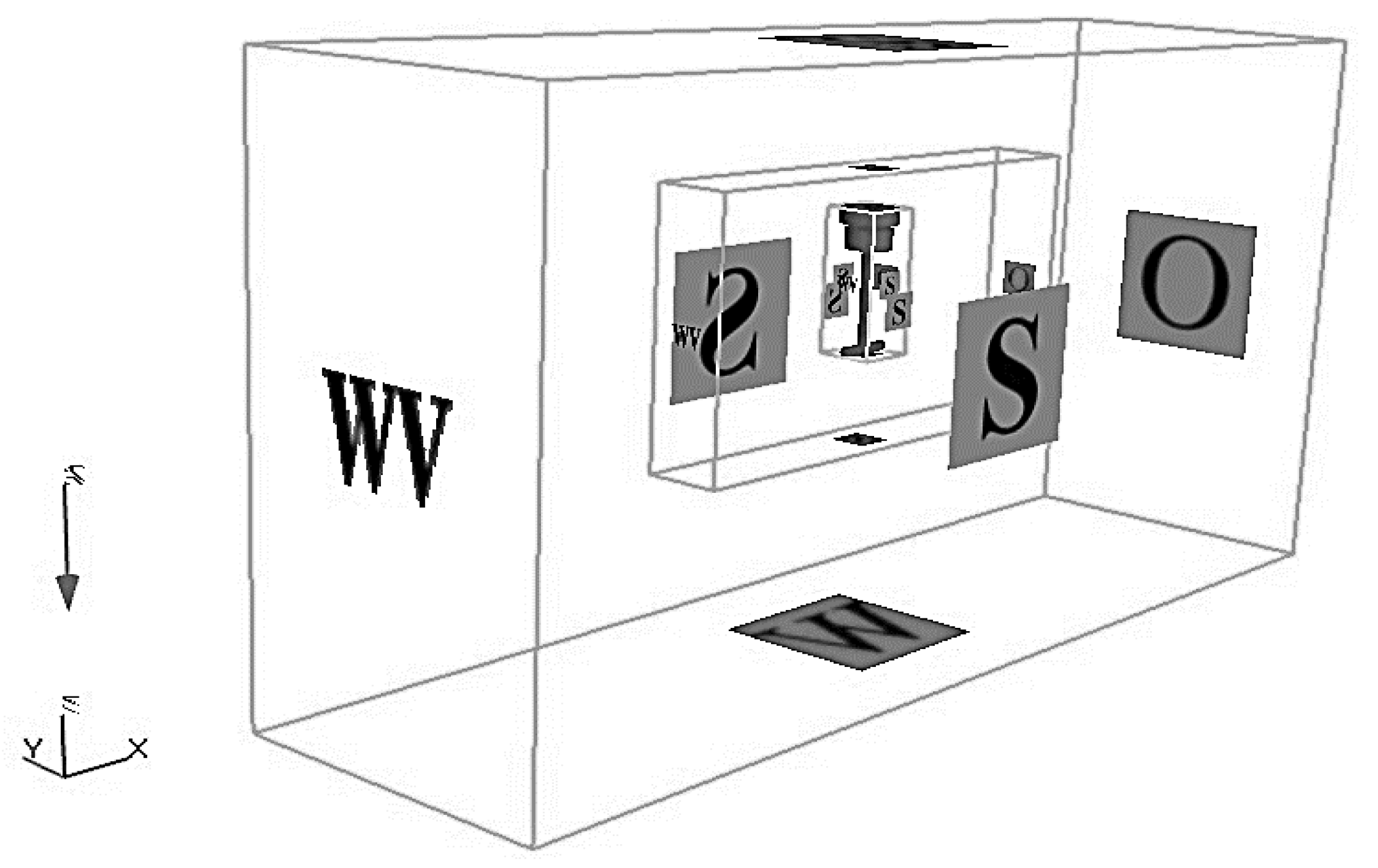
In this equation, A shows the wave amplitude which is gained from He’s study [23]. The other wave characteristics were assumed constant. In addition to consider sine wave as an inlet of the specific control volume, other boundary conditions are shown in Figure 3.
As shown in Figure 3, “VW” is a linear wave inlet of the control volume, “S” is the symmetric condition for three different walls, “W” is a wall with slip boundary condition, and “O” is the outflow when the water is not allowed to enter the outflow boundary. The reason for using three different domains for a numerical solution is to use different grid sizes. Whatever goes inside the blocks, the grid size becomes smaller because computational accuracy is more essential than outer blocks in this region. As such, the inner block has the smallest grid size among the others. Similar to the other computational fluid dynamic studies, grid generation and independencies should be analyzed to find a suitable grid size which has the best accuracy due to the least computational time, which is shown in Table 1.
As presented in Table 1, the best selected total grid is 5,000,000 grids due to the related accuracy. It shows that this grid size can be selected because it is as accurate as 7,000,000 grids, due to the fact that it has higher computing speed and lower computational cost. Furthermore, it presents the accuracy in displacement for each grid size during the whole of the calculation time when input wave height is assumed as 1 m [31]. According to the harmonic linear motion of a buoy in a chamber, the special generator will convert these motions to electricity by utilizing Faraday’s law of induction.
2.5. Machine Learning LSTM Method of Prediction
The electrical power of ocean waves forecasting models has become stable and highly credible after decades of considerable improvements. However, the models require a large amount of data to train, which usually takes a longer time, even for a small-scale forecast. For that reason, machine learning and deep learning algorithms emerged to improve accuracy and promptness of the prediction. Recurrent Neural Network (RNN) are types of Neural Networks designed to use sequential data, such as time-series. In RNNs, outputs can be fed back into the network as inputs, creating a recurrent structure. RNNs are trained by backpropagation. During backpropagation, RNNs suffer from a gradient vanishing problem. The gradient is the value used to update Neural Networks’ weight. The gradient vanishing problem is when a gradient shrinks as it back-propagates through time. Therefore, layers that obtain a small gradient do not learn and cause the network to have short-term memory [32].
Long Short-Term Memory (LSTM) is a specialized RNN to mitigate the gradient vanishing problem. LSTMs can learn long-term dependencies using a mechanism called gates. Figure 4 presents the architecture of an LSTM cell. These gates can learn what information in the sequence is important to keep or throw away. LSTMs have three gates—input, forget and output [33].
To save the data information that is utilized in the specific storage within hidden layers, the “cell” has been introduced. As presented in Equations (11) and (12), and indicate the input gate and forget gate for controlling each cell state [34].
where g indicates a nonlinear sigmoid function for activation procedure; i and f indexes represent the input and forget parameters; W and b present the weight matrix and bias function; ht−1 introduces the output vector of the last time step; and Xt shows the input vector of the current time step.
Equation (13) presents the relation to obtain an input’s current state.
As shown in Equation (13), c index introduces the recent state of each parameters. Equation (14) describes the current cell that i is considered to utilize both the forget and input gates.
By using the output gate of each cell as is written in Equation (15), the output of the whole network of a long short-term memory has been presented as Equation (16).
o index introduces the cell output parameters.
The essential task in algorithm designing procedures of neural network is to select the best number of neurons and relative layers. In machine learning systems which contain neurons, the connection links between them are introduced as weighted activation. According to proposed usage, it was modeled by the input layer. To analyze procedure, hidden layers were used by considering several neurons which transferred data from input to output neuron. The network’s dataset was split into training and testing sets. The main crucial task in optimization is to minimize the difference between predicted and actual data [4,35]. The LSTM model has been utilized with 10 LSTM layers of 10 neurons and “Sigmoid” as an activation function. The optimized train size is 90% of a total 591 input data and the test size is 10%. Furthermore, the epoch size is seven and walk-forward validation methods were used. The back-propagation algorithm was utilized for the administrated learning technique [36]. Figure 5 shows the neural network details which are used in this research.
As presented in Figure 5, the recent study utilized a proposed LSTM Network with input layer time-series parameters which were followed by an LSTM layer. These layers learn the relation between different parameters in time steps and serialized input data. Moreover, during each of the layers, the LSTM layer’s neuron is connected to the next layer’s neuron for each LSTM cell. The artificial intelligence predictions have been performed by utilizing equations of the LSTM method. Hence, decreasing rank procedure of the input data was performed by a Mahalanobis distance (MD) method to reduce the predicting time of the overall procedure. Our study is a kind of regression prediction which can find a relation between the input and output data. Table 2 presents the LSTM parameters which were introduced as effective parameters on output generated power of the Searaser.
In this study, by using numerical solutions, the collected dataset from simulation and experimental study was imported to the LSTM Network, and then it predicted the output parameters. Next, the data that was gained by numerical solution was compared with the predicted data from the LSTM method. Finally, the correlation matrix was applied on a recognition step of the occurrence of faults.
3. Results and Discussion
This section describes the results of the evaluation of the wave power generation prediction based on the proposed LSTM Network. Accordingly, the result of numerical solutions and the prediction plots of correlation parameters were presented and compared with each other. Furthermore, the Searaser’s performance was demonstrated for various input linear–sine waves, the information of which exists in Figure 3. The wave height moves the buoy in z direction and its motion will be converted into electricity. Equation (9) demonstrates that the output power depends on the wave height and wave period of each time. Furthermore, the other parameters become constant during the simulation. Figure 6 shows the numerical solution of the simulation. It shows the relation of the generated power with the whole simulation time.
The instability of the generating power at different times during the simulation is presented. This is caused by the variation of wave heights. To illustrate the correlation between all of the effective variables with the LSTM method further, the predicted plots were presented as a matrix of figures. The scatter plot of predicted magnitudes was shown in Figure 7. The figure presents a matrix whose intersection of each row and column shows a graph depicting the relationship between the two parameters. Using this type of display causes the dependence of all parameters on each other to be well shown.
As presented in Figure 7, the correlation of different parameters is shown as scatter figures. Figure 8 is a more comprehensive type of Figure 7. As Figure 8 shows, the gradient descent for both parameters in each curve is calculated, which can be reached in Figure 7 by connecting the extreme points of each curve.
To find a higher correlated parameter among others neglected during predicting procedure, the correlation matrix could be prepared as Figure 9. This matrix shows the relation of different quantities, with a heat-map visualization method. It demonstrates the magnitudes with colors, from a lighter to a darker one. The lighter color shows the best relation, so it is easy to infer that the prediction procedure finds a good relation between wave height and power.
For comparative analysis, it is necessary to compare the predicted production power graphs with numerical solution values to prove the efficiency of this method in using this field, as shown in Figure 9 and Figure 10. For this reason, Figure 10 shows the power curve in terms of simulation time. It presents the bar-graph, the differences between two type of values is quite apparent.
To evaluate the results of the simulation, it is necessary to make a comparison with another study. Figure 11 shows that, to achieve larger powers, it is necessary for wavelengths with higher altitudes to collide with the wave converter. Furthermore, the main claim of our study is to introduce a relation between the generated power and wave height. For this purpose, the output data of the LSTM method were used and compared with numerical analysis, which was performed by simulation software. Furthermore, it presents this relation and the curve fitting operation, and the mathematical relation introduced as a power function.
As shown in Figure 11, the recent study is compared with Babajani’s study [31]. Among the differences between the results, we can point to a different input. Wider inputs are used, and the results are more acceptable. The difference in the numerical results obtained from the simulation is only 0.05%, and this shows that the results can be trusted. As can be deduced from the comparison of the curves obtained in Figure 11, there is a good match between the two methods of numerical solution and LSTM. Numerical solution takes 4 days 1 h, but predicting results by artificial intelligence takes only 2 min and 23 s. By obtaining mathematical equations from figure diagrams, a relation can be provided that the replace a numerical solution can be used to increase the speed and accuracy during simulation. Regarding scalability, one important aspect is to assess power extraction by the Searaser in the same real scale. This is due to the fact, in this study, the Searaser was numerically simulated by the data extracted from the patent scale. Therefore, the scale was 1:1 and the simulation results were close to reality. Furthermore, the data were curve fitted and two mathematical relations were presented to attribute the output power by the Searaser converter and the wave height, one of which was the relation provided by Babajani [31], and the other the relation presented by recent research. Equations (17) and (18) represent y1 and y2 in Figure 11.
In the following, we will examine one of the objectives of this study, which is the power diagram in terms of wind speed. Figure 12 shows this relationship extracted from the LSTM method.
As can be deduced from Figure 12, the data frequency is low wind speed, and this chart is a reliable way to predict similar models because it is a combination of experimental card and simulation data modeled by artificial intelligence. To represent the effect of selected parameter, the respective comparative analysis is displayed here. Root mean square error (RMSE) of these relations is presented in Table 3. Table 3 shows that there is a good agreement between two utilized methods, and it can be concluded that the LSTM method is much faster and more accurate in predicting values.
4. Conclusions
In this study, the power characteristics of a Searaser are presented by analyzing numerical and experimental data. An LSTM network has been developed for predicting the power output of the Searaser. By capability of the proposed LSTM prediction method, there can also be a relationship found between wind speed and the output power of the Searaser. According to the obtained results and the comparison between the two methods studied, it can be inferred that the LSTM network is able to predict power in terms of height more accurately and faster than the numerical solution, and these were in a good agreement with the result of the numerical analysis. The comparison between the two methods shows that results of the machine learning method are so accurate and RSME value of the parameters are 0.49 as a mean value. This study makes progress on energy management and investment for tidal renewable energy systems. The present study also exhibits some limitations, which open paths for future research. Therefore, this study can be improved by analyzing more effective parameters on output power of ocean waves, such as temperature, climate change, etc. Moreover, better results can be achieved by using accurate methods, as well as developing and upgrading WEC systems.
Author Contributions
S.M.M. and M.G. did the conceptualization; M.D.M. and S.M.M. completed the simulation. Methodology, S.M.M. and A.M.; software, S.M.M. and M.D.M.; supervision, M.G.; administration, A.M. The manuscript was written and reviewed through equal contributions of all the authors. All authors have read and agreed to the published version of the manuscript.
Funding
This research received no funding.
Institutional Review Board Statement
Not applicable.
Informed Consent Statement
Not applicable.
Data Availability Statement
Data is available through the corresponding author with a reasonable request.
Acknowledgments
Open Access Funding by the Publication Fund of the TU Dresden. Amir Mosavi would like to thank Alexander von Humboldt Foundation.
Conflicts of Interest
The authors declare no conflict of interest.
References
- Arutyunov, V.S.; Lisichkin, G.V. Energy resources of the 21st century: Problems and forecasts. Can renewable energy sources replace fossil fuels? Russ. Chem. Rev. 2017, 86, 777–804. [Google Scholar] [CrossRef]
- Perera, F. Pollution from fossil-fuel combustion is the leading environmental threat to global pediatric health and equity: Solutions exist. Int. J. Environ. Res. Public Health 2018, 15, 16. [Google Scholar] [CrossRef] [PubMed] [Green Version]
- Sinsel, S.R.; Riemke, R.L.; Hoffmann, V.H. Challenges and solution technologies for the integration of variable renewable energy sources—A Review. Renew. Energy 2020, 145, 2271–2285. [Google Scholar] [CrossRef]
- Aderinto, T.; Li, H. Ocean wave energy converters: Status and challenges. Energies 2018, 11, 1250. [Google Scholar] [CrossRef] [Green Version]
- Jiang, B.; Li, X.; Chen, S.; Xiong, Q.; Chetn, B.-F.; Parker, R.G.; Zuo, L. Performance analysis and tank test validation of a hybrid ocean wave-current energy converter with a single power takeoff. Energy Convers. Manag. 2020, 224, 113268. [Google Scholar] [CrossRef]
- Ahamed, R.; McKee, K.; Howard, I. Advancements of wave energy converters based on power take off (PTO) systems: A review. Ocean Eng. 2020, 204, 107248. [Google Scholar] [CrossRef]
- Ocean Energy Systems. Annual Report Ocean Energy Systems 2016. Ocean Energy Systems Website. 2017. Available online: https://report2016.ocean-energy-systems.org (accessed on 21 December 2020).
- Ruehl, K.; Forbush, D.D.; Yu, Y.-H.; Tom, N. Experimental and numerical comparisons of a dual-flap floating oscillating surge wave energy converter in regular waves. Ocean Eng. 2020, 196, 106575. [Google Scholar] [CrossRef]
- Giorgi, G.; Gomes, R.P.; Henriques, J.C.; Gato, L.M.; Bracco, G.; Mattiazzo, G. Detecting parametric resonance in a floating oscillating water column device for wave energy conversion: Numerical simulations and validation with physical model tests. Appl. Energy 2020, 276, 115421. [Google Scholar] [CrossRef]
- Shahriar, T.; Habib, M.A.; Hasanuzzaman, M.; Shahrear-Bin-Zaman, M. Modelling and optimization of Searaser wave energy converter based hydroelectric power generation for Saint Martin’s Island in Bangladesh. Ocean Eng. 2019, 192, 106289. [Google Scholar] [CrossRef]
- Reikard, G.; Robertson, B.; Bidlot, J.-R. Wave energy worldwide: Simulating wave farms, forecasting, and calculating reserves. Int. J. Mar. Energy 2017, 17, 156–185. [Google Scholar] [CrossRef]
- Pena-Sanchez, Y.; Garcia-Abril, M.; Paparella, F.; Ringwood, J.V. Estimation and forecasting of excitation force for arrays of wave energy devices. IEEE Trans. Sustain. Energy 2018, 9, 1672–1680. [Google Scholar] [CrossRef] [Green Version]
- Sang, Y.; Karayaka, H.B.; Yan, Y.; Yilmaz, N.; Souders, D. 1.18 Ocean (Marine) Energy. In Comprehensive Energy Systems; Dincer, I., Ed.; Elsevier: Amsterdam, The Netherlands, 2018; Volume 1, pp. 733–769. [Google Scholar]
- Reikard, G.; Robertson, B.; Bidlot, J.-R. Combining wave energy with wind and solar: Short-term forecasting. Renew. Energy 2015, 81, 442–456. [Google Scholar] [CrossRef]
- Bento, P.; Pombo, J.; Mendes, R.; Calado, M.; Mariano, S. Ocean wave energy forecasting using optimised deep learning neural networks. Ocean Eng. 2021, 219, 108372. [Google Scholar] [CrossRef]
- Ni, C.; Ma, X. Prediction of wave power generation using a convolutional neural network with multiple inputs. Energies 2018, 11, 2097. [Google Scholar] [CrossRef] [Green Version]
- Liu, Z.; Wang, Y.; Hua, X. Prediction and optimization of oscillating wave surge converter using machine learning techniques. Energy Convers. Manag. 2020, 210, 112677. [Google Scholar] [CrossRef]
- Li, L.; Gao, Y.; Ning, D.; Yuan, Z.M. Development of a constraint non-causal wave energy control algorithm based on artificial intelligence. Renew. Sustain. Energy Rev. 2020, 138, 110519. [Google Scholar] [CrossRef]
- Gómez-Orellana, A.M.; Fernández, J.C.; Dorado-Moreno, M.; Gutiérrez, P.A.; Hervás-Martínez, C. Building suitable datasets for soft computing and machine learning techniques from meteorological data integration: A case study for predicting significant wave height and energy flux. Energies 2021, 14, 468. [Google Scholar] [CrossRef]
- Butt, F.M.; Hussain, L.; Mahmood, A.; Lone, K.J. Artificial Intelligence based accurately load forecasting system to forecast short and medium-term load demands. Math. Biosci. Eng. 2020, 18, 400–425. [Google Scholar] [CrossRef] [PubMed]
- Cheng, Y.; Xu, C.; Mashima, D.; Thing, V.L.; Wu, Y. PowerLSTM: Power demand forecasting using long short-term memory neural network. In Proceedings of the International Conference on Advanced Data Mining and Applications, Singapore, 5–6 November 2017; Springer: Cham, Switzerland, 2017. [Google Scholar]
- Lin, Z.; Cheng, L.; Huang, G. Electricity consumption prediction based on LSTM with attention mechanism. IEEJ Trans. Electr. Electron. Eng. 2020, 15, 556–562. [Google Scholar] [CrossRef]
- Ni, C.; Ma, X.; Wang, J. Integrated deep learning model for predicting electrical power generation from wave energy converter. In Proceedings of the 2019 25th International Conference on Automation and Computing, Lancaster, UK, 5–7 September 2019. [Google Scholar]
- He, J. Coherence and cross-spectral density matrix analysis of random wind and wave in deep water. Ocean Eng. 2020, 197, 106930. [Google Scholar] [CrossRef]
- Smith, A. Pumping Device. Patent Application Publication. U.S. Patent US 2013/0052042 A1, 28 February 2013. [Google Scholar]
- Pedrycz, W.; Skowron, A.; Kreinovich, V. Handbook of Granular Computing; John Wiley & Sons: Hoboken, NJ, USA, 2008. [Google Scholar]
- Bhinder, M.; Mingham, C.; Causon, D.; Rahmati, M.; Aggidis, G.; Chaplin, R. Numerical and experimental study of a surging point absorber wave energy converter. In Proceedings of the 8th European Wave and Tidal Energy Conference, Uppsala, Sweden, 7–10 September 2009. [Google Scholar]
- Gomes, R.P.; Henriques, J.C.; Gato, L.M.; Falcão, A.D. Hydrodynamic optimization of an axisymmetric floating oscillating water column for wave energy conversion. Renew. Energy 2012, 44, 328–339. [Google Scholar] [CrossRef]
- Hirt, C. Flow-3D User’s Manual; Flow Sciences, Inc.: Leland, NC, USA, 1988. [Google Scholar]
- Elsayed, M.A. Wavelet bicoherence analysis of wind–wave interaction. Ocean Eng. 2006, 33, 458–470. [Google Scholar] [CrossRef]
- Babajani, A. Hydrodynamic performance of a novel ocean wave energy converter. Am. J. Fluid Dyn. 2018, 8, 73–83. [Google Scholar]
- López, E.; Valle, C.; Allende, H.; Gil, E.; Madsen, H. Wind power forecasting based on echo state networks and long short-term memory. Energies 2018, 11, 526. [Google Scholar] [CrossRef] [Green Version]
- Duan, Y.; Yisheng, L.; Wang, F.-Y. Travel time prediction with LSTM neural network. In Proceedings of the 2016 IEEE 19th International Conference on Intelligent Transportation Systems, Rio de Janeiro, Brazil, 1–4 November 2016. [Google Scholar]
- Ma, X.; Tao, Z.; Wang, Y.; Yu, H.; Wang, Y. Long short-term memory neural network for traffic speed prediction using remote microwave sensor data. Transp. Res. Part C Emerg. Technol. 2015, 54, 187–197. [Google Scholar] [CrossRef]
- Li, H. (Ed.) Wave Energy Potential, Behavior and Extraction; MDPI: Basel, Switzerland, 2020. [Google Scholar]
- Nezhad, M.M.; Groppi, D.; Rosa, F.; Piras, G.; Cumo, F.; Garcia, D.A. Nearshore wave energy converters comparison and Mediterranean small island grid integration. Sustain. Energy Technol. Assess. 2018, 30, 68–76. [Google Scholar]
Figure 1.
The wind speed and wave height fluctuation in simulation time.

Figure 2.
The cross-section of a Searaser, introducing different components.

Figure 3.
Different boundary conditions of numerical solution.

Figure 4.
The architecture of an LSTM cell.

Figure 5.
The specific neural network of recent study.

Figure 6.
The variation of generated power with simulation time.

Figure 7.
The correlation of different parameters with each other.

Figure 8.
The linearization of scatter data within the correlation of different parameters with each other.
Figure 8.
The linearization of scatter data within the correlation of different parameters with each other.

Figure 9.
The correlation matrix of different parameters with each other.

Figure 10.
Comparative analysis of the numerical solution and LSTM method.

Figure 11.
The relation between generated electrical power with wave height.

Figure 12.
The relationship between output power and wind speed.


Table 1.
The grid generation information.
| Title | 1 | 2 | 3 |
|---|---|---|---|
| Mesh block (Number 1) |  |  |  |
| Total number of elements | 7,000,000 | 5,000,000 | 1,000,000 |
| Run time | 5 days 7 h | 4 days 1 h | 2 days 20 h |
| The accuracy of Searaser displacement parameter | 95% | 93% | 85% |
Table 2.
The detailed information of LSTM method.
| LSTM Parameters | Recent Study Parameters |
|---|---|
| Input parameters 1. Wave height 2. Time 3. Wind slow velocity 4. Number | |
| Output parameters 1. Generated power |
Table 3.
The RMSE value of analyzing different variables.
| Analysis Variables | RSME Value |
|---|---|
| Power output, wave height | 0.56 |
| Power output, simulation time | 0.42 |
| Power output, wave height, simulation time | 0.49 |
Publisher’s Note: MDPI stays neutral with regard to jurisdictional claims in published maps and institutional affiliations. |
© 2021 by the authors. Licensee MDPI, Basel, Switzerland. This article is an open access article distributed under the terms and conditions of the Creative Commons Attribution (CC BY) license (https://creativecommons.org/licenses/by/4.0/).
Share and Cite
MDPI and ACS Style
Mousavi, S.M.; Ghasemi, M.; Dehghan Manshadi, M.; Mosavi, A. Deep Learning for Wave Energy Converter Modeling Using Long Short-Term Memory. Mathematics 2021, 9, 871. https://doi.org/10.3390/math9080871
AMA Style
Mousavi SM, Ghasemi M, Dehghan Manshadi M, Mosavi A. Deep Learning for Wave Energy Converter Modeling Using Long Short-Term Memory. Mathematics. 2021; 9(8):871. https://doi.org/10.3390/math9080871
Chicago/Turabian StyleMousavi, Seyed Milad, Majid Ghasemi, Mahsa Dehghan Manshadi, and Amir Mosavi. 2021. "Deep Learning for Wave Energy Converter Modeling Using Long Short-Term Memory" Mathematics 9, no. 8: 871. https://doi.org/10.3390/math9080871
Note that from the first issue of 2016, this journal uses article numbers instead of page numbers. See further details here.