Queuing-Inventory Models with MAP Demands and Random Replenishment Opportunities

Abstract

Combining the study of queuing with inventory is very common and such systems are referred to as queuing-inventory systems in the literature. These systems occur naturally in practice and have been studied extensively in the literature. The inventory systems considered in the literature generally include $(s,S)$-type. However, in this paper we look at opportunistic-type inventory replenishment in which there is an independent point process that is used to model events that are called opportunistic for replenishing inventory. When an opportunity (to replenish) occurs, a probabilistic rule that depends on the inventory level is used to determine whether to avail it or not. Assuming that the customers arrive according to a Markovian arrival process, the demands for inventory occur in batches of varying size, the demands require random service times that are modeled using a continuous-time phase-type distribution, and the point process for the opportunistic replenishment is a Poisson process, we apply matrix-analytic methods to study two of such models. In one of the models, the customers are lost when at arrivals there is no inventory and in the other model, the customers can enter into the system even if the inventory is zero but the server has to be busy at that moment. However, the customers are lost at arrivals when the server is idle with zero inventory or at service completion epochs that leave the inventory to be zero. Illustrative numerical examples are presented, and some possible future work is highlighted.

1. Introduction

Models for inventory management under uncertainty have been studied extensively. The two key questions of when and how many to order have been addressed under a variety of factors such as the nature of inventory review (continuous or periodic), order quantity (fixed or variable), lead time for an order to be fulfilled (negligible, constant or random), nature of demand (deterministic or random), and other factors to optimize a function of various costs such as ordering, carrying inventory, lost sales, etc.

Most models assume a single supplier and fixed cost of replenishment. Some models incorporate the availability of random opportunities for replenishment which may lower system costs due to reduced unit cost and/or ordering cost. We refer to them as opportunistic replenishment. Friend [1] studied systems with special opportunities occurring according to a Poisson process. These opportunities, which may be exercised only at the instant of their occurrence, are offered for the same unit price but at reduced or zero ordering cost. Hurter and Kaminsky [2] extend this model to systems where the special opportunities may be exercised during a random period. Silver, Robb, and Rahnama [3] developed an efficient heuristic for the Hurter and Kaminsky [2] model. Gurnani [4] considered periodic review systems and used game theory to study the economics of placing a special order between reviews if a discounted sale is offered. Moinzadeh [5] considered systems with constant demand rate, zero lead time, and special discounted opportunities occurring at exponentially distributed intervals, and obtained optimal order quantity at regular price when inventory reaches zero, and the threshold and order quantity at discounted price. Feng and Sun [6] suggest modifying the $(s,S)$ policy to a four-parameter system (threshold and order quantity for regular and discount purchases) and proposed a bisection search procedure to determine the optimal values of the four parameters. Goh and Sharafali [7] consider the model in [1,2] and incorporate the policy of passing the cost reduction due to special purchases downstream to increase demand. Chaouch [8] considers the model in [1,2] when special and regular prices are valid over alternating exponential intervals. Tajbakhsh and Zolfaghari [9] consider systems with discounts offered at exponential intervals with the discount price given by a discrete random variable and develop optimal order quantities at each special price and further extended the model to the case of multiple suppliers. Karimi-Nasab and Konstantaras [10] consider a system with constant demand, periodic random review intervals (uniformly distributed or exponential subject a maximum and minimum) and random special sale offers, and determine maximum inventory level for regular purchases, and a higher maximum for special purchases. Den Boer and Zwart [11] consider a system where the management makes simultaneous decisions on whether to take advantage of the special discounted offer, and the selling price of a unit similar to [7]. All the above references assume that the lead time for receiving a special replenishment is negligible.

In all the above models, it is assumed that the special opportunities for replenishment are always considered as a supplement to the normal replenishment process. In many situations such as drugstores, groceries, small supermarkets, etc., the suppliers visit the retailers at random (but frequent) intervals to offer special sales. This raises the possibility that for some systems it may be more economical to manage inventory solely based on special offers. This is particularly attractive for non-critical items (e.g., canned goods, generic medication) where stock outs are not critical. Special replenishment opportunities offer lower unit cost and/or reduced ordering cost, and are usually available without delay.

Inventory models discussed above assume that the time to process a demand is negligible. In many situations, completing a customer’s service requires other resources, in addition to the item(s) in inventory (e.g., requiring a pharmacist to process the sale for prescription medication). Such inventory systems are referred to as queuing-inventory (QI) models or inventory models with positive service time, and have received a great deal of attention recently. Research in queuing-inventory systems may be classified based on features such as the nature of customer arrival process, service time distribution, server vacation, service discipline, customer behavior, inventory review policy, replenishment policy, stock-out assumptions, perishability of units, lead time for replenishment, among others. We refer the readers to Krishnamurthy, Shajin, and Narayanan [12] for a general review of queuing-inventory models, to Choi et al. [13] for a survey of QI models with phase-type service times, and to Melikova and Shahmaliyeva [14] for a discussion of QI models for perishable items. Recent generalizations of QI models are due to Chakravarthy, Maity and Gupta [15], who studied a QI model in which the service is carried out in batches, Chakravathy [16], who studied a QI model in which the demand occurs in batches, and Chakravarthy and Rumyantsev [17], who study a QI system with batch demand, Markovian Arrival Process (MAP), and phase-type service time and exponential replenishment lead times.

In this paper, we explore queuing-inventory systems which solely use special opportunities for replenishment. This research is at the interface of the two areas of traditional inventory systems, and the queuing-inventory systems. Most traditional inventory models consider the demand to occur one unit at a time, at either constant or exponential intervals. Our models extend this to consider demand that can occur in batches of random size, with arrivals following a very general process which allows for a broad class of inter-arrival times and autocorrelation between inter-arrival times. For both types of inventory systems, it is a significant departure to manage inventory exclusively based on random replenishment opportunities. The objective of this study was to understand the behavior of such systems and compare them with the traditional $(s,S)$-type inventory management systems.

2. General Description

The customer arrivals are modeled using Neuts’ versatile Markovian point process, now referred to as batch Markovian arrival process ($BMAP$). If customers arrive one at a time, the process is referred to as Markovian arrival process or briefly $MAP$. While the customers arrive singly to the service facility, but their demands for inventory items are in varying sizes. One of the major advantages of using $MAP$ to model the arrival process is to capture any correlation present in successive arrivals. The $MAP$ is completely described by two parameter matrices, say, $(E_0,E_1)$ of dimension m. While, $E_0$ governs transitions within the underlying Markov process with generator $E=E_0+E_1$, the transitions governed by $E_1$ correspond to the arrivals of customers. We assume that E is an irreducible generator. $MAP$ and $BMAP$ have been extensively used in stochastic model and there is a vast literature available on these. We refer the reader to [18,19,20,21,22,23,24,25,26,27,28,29] for details on $MAP$ and $BMAP$ and other key references.

Each customer demands a random number of items from inventory before being processed by a single server. At the instant of an arrival, the available inventory is reduced by the amount demanded by the customer. The number of remaining items in inventory is referred to as available to promise or ATP in the business community. In this paper, we always refer to ATP when referring to inventory. Physical inventory is not relevant because once allocated to a customer, a unit is no longer available.

When the inventory level is positive, but less than the number of units demanded by a customer, the customer’s demand is partially satisfied and the inventory level is set to zero. Arrivals to the system when inventory level is zero, are denied entry and are lost. The time to service a customer has a phase-type or $PH$-distribution and is independent of the number of units demanded. For details on $PH$-distributions and their usefulness in stochastic modeling, we refer the reader to [29,30,31].

Opportunities to replenish the inventory occur according to a Poisson process. We assume that the lead time associated with a replenishment is zero. Replenishment decisions are based on two parameters K and L ($0\le L<K<\infty$) and for convenience we refer to the policy as a $(K,L)$ policy. If the inventory at the time a replenishment opportunity becomes available is equal to i, a replenishment order to bring the inventory level to K is placed with probability 1 if $i\le L$, and with with probability $a_{i-L}$ if $L<i<K$.

In this paper, we consider two types of models, referred to as Opportunistic Model 1 and Opportunistic Model 2, and these are described in the following sections.

Any queuing-inventory model with positive service time can be looked at two different ways according to these two models to see which one will be better from either customer or management or from both points of view. Therefore, there is a trade-off between the two models and a comparison of these would benefit practicing managers to make a decision on the choice of the models.

We use the classical matrix-analytic method (see, e.g., [30]) to formulate the associated stochastic process with matrix-geometric steady-state probability vector. Performance measures of interest are obtained in terms of the steady-state probabilities.

The structure of the present paper is as follows. Models 1 and 2 are analyzed in Section 3 and Section 4, respectively. Some selected system performance measures are presented in Section 3.2 and Section 4.2. In Section 5, we numerically study the key performance measures of both models in steady-state as well as present a cost analysis to compare the two models. Some concluding remarks are noted in Section 6. The following notation is used in the paper.

• The subscript $i,i=1,2$ refers to the model under consideration.
• The symbol ${}^{\prime }$ stands for the transpose notation.
• The notations ⊗ and ⊕ stand for the Kronecker product and Kronecker sum, respectively (see, e.g., [32,33]).
• $e^{\prime }=(1,1,\cdots ,1)$, whose dimension should be clear in the context. Where more clarity is needed, the dimension will be mentioned, e.g., $e\left(m\right)$ is a column vector of 1s of dimension m.
• ${e^{\prime }}_i=(0,0,\cdots ,1,0,\cdots ,0)$, where 1 is in the ith position.
• I denotes an identity matrix, whose dimension is dictated by the context.
• $\Delta (E_1,\cdots ,E_r)$ denotes a diagonal matrix with diagonal (possibly block) entries given by $E_1$ through $E_r$. In the context where this notation is used, it will be clear whether the entities are scalars or vectors or matrices.

3. Opportunistic Model 1

In this first model, we consider the scenario where the customers arrive to a service facility consisting of a single server. The arrivals are modeled using Neuts’ versatile Markovian point process, now referred to as batch Markovian arrival process ($BMAP$). While the customers arrive singly to the service facility, their demands for inventory items are in varying sizes. The $MAP$ parameter matrices describing the arrivals of customers are $(E_0,E_1)$ of dimension m. The customers’ demands are in batches of varying sizes. Suppose that M denotes the demand size. We assume that M has the following discrete distribution on finite support,

$$P(M=i)=p_i,1\le i\le N,\sum _{i=1}^N{p}_i=1.$$

(1)

In order to determine the arrival rate of the customers to the system, we first define the invariant vector of the generator $E=E_0+E_1$ that governs the underlying Markov process for the arrivals. Suppose that $\mathbf{\theta }$ is the invariant probability vector of E. That is,

$$\mathbf{\theta }E=0,\mathbf{\theta }e=1.$$

(2)

Then, the arrival rate of the customers is given by

$$\lambda =\mathbf{\theta }{E}_{1}e.$$

(3)

Let ${\mu }_M$ to be the mean of the demand size of each customer. That is,

$${\mu }_M=\sum _{i=1}^{N}i{p}_i.$$

(4)

In this paper, we assume that the demands of the customers are either fully met or partially met or not met at all, depending on, respectively, if the demands in the inventory are fully adequate, partially adequate, or the inventory level is zero. When the inventory level is zero at the time of the arrival of a customer, the arriving customer will be lost.

The size of the inventory is assumed to be finite with a capacity to hold at most K items. As described and motivated earlier, the main purpose of this paper was to incorporate opportunistic replenishment into stochastic models dealing with queues with inventory and positive services. The opportunistic events occur according to a Poisson process with parameter $\gamma$. Therefore, when an opportunity occurs for replenishing the inventory, the system has the ability to bring the current inventory level to the maximum level through a given probability structure. Suppose that the inventory level at the time a replenishment opportunity is i. Then, the opportunity will be availed to bring the inventory level to K with probability 1 if $i\le L$; however, if $i>L$, then with probability $a_{i-L},0\le a_{i-L}<1$, the opportunity will be availed to bring the inventory to K, for $L<i\le K-1$.

When a customer enters the system (either with fully or partially met demands), the inventory level will be reduced by that customer’s demand size. Note that the only way an arriving customer will be lost is when the inventory level is zero at that moment. However, customers have to wait until their demands are processed with a positive service time, which is assumed to be random. The services follow a phase-type $\left(PH\right)$-distribution with representation $(\mathbf{\beta },S)$ of order n. Note that the mean service rate, say, $\mu$, is given by

$$\mu ={\left[\mathbf{\beta }{(-S)}^{-1}e\right]}^{-1}.$$

(5)

For use in sequel, we define $S^0=-Se$.

Suppose we define the quantities:

• $J_1\left(t\right)$ to be the number of customers in the system (including one in service),
• $J_2\left(t\right)$ to be the level of the inventory,
• $J_3\left(t\right)$ to be the phase of the service (if the server is idle, this will not be defined),
• $J_4\left(t\right)$ to be the phase of the arrival process,

at time t. The Markov process $\{(J_1\left(t\right),J_2\left(t\right),J_3\left(t\right),J_4\left(t\right)):t\ge 0\}$ is a quasi-birth-and-death process $\left(QBD\right)$ with state space given by

$$\begin{array}{c}{\Omega }_1=\{(0,j,r):0\le j\le K,1\le r\le m\}\\ \bigcup \left\{\right((i,j,k,r):0\le j\le K,1\le k\le n,1\le r\le m,i\ge 1\}.\end{array}$$

We now define the levels based on the set of states defined above. Suppose that $0=\left\{\right(0,j,r):0\le j\le K,1\le r\le m\}$ and $i=\left\{\right(i,j,k,r):0\le j\le K,1\le k\le n,1\le r\le m\},i\ge 1$. This way, we notice that 0 corresponds to an idle system while i corresponds to the system having i customers with one in service, and the inventory, and the arrival process are in various states. For use in the sequel, we define a few additional notations.

• ${\widehat{p}}_i$, probabilities of demands greater than i, are computed as

  $${\widehat{p}}_i=\sum _{k=i+1}^N{p}_k,1\le i\le N-1.$$

  (6)
• P, a square matrix of dimension $K+1$ is defined as

  $$P=\left[\begin{array}{ccccccc}0& 0& 0& \cdots & 0& 0& 0\\ 1& 0& 0& \cdots & 0& 0& 0\\ {\widehat{p}}_1& p_1& 0& \cdots & 0& 0& 0\\ {\widehat{p}}_2& p_2& p_1& \cdots & 0& 0& 0\\ ⋮& ⋮& ⋮& \cdots & ⋮& ⋮& ⋮\\ {\widehat{p}}_{N-1}& p_{N-1}& p_{N-2}& \cdots & 0& 0& 0\\ 0& p_N& p_{N-1}& \cdots & 0& 0& 0\\ 0& 0& p_N& \cdots & 0& 0& 0\\ ⋮& ⋮& ⋮& \cdots & ⋮& ⋮& ⋮\\ 0& 0& 0& \cdots & p_2& p_1& 0\end{array}\right].$$

  (7)
  A quick look at P indicates that the customers’ demands are taken into consideration at the time of their arrivals. The first column of P justifies that the structure due to the customers’ demands are met partially. It is easy to verify that

  $$Pe={(0,1,\cdots ,1)}^{\prime }.$$

  (8)

The generator, $Q_1$, of the $QBD$-process for Opportunistic Model 1 is given by (note that blank spaces correspond to the entries are zero)

$$Q_1=\left(\begin{array}{cccccc}B& P\otimes \mathbf{\beta }\otimes E_1& & & & \\ I\otimes S^0\otimes I& A_1& A_0& & & \\ & A_2& A_1& A_0& & \\ & & A_2& A_1& A_0& \\ & & & \ddots & \ddots & \ddots \end{array}\right).$$

(9)

For a better display of the matrices, we take

$$\begin{array}{ccc}F\hfill & =\hfill & E-\gamma I,\hfill \\ F_0\hfill & =\hfill & E_0-\gamma I,\hfill \\ F_r\hfill & =\hfill & E_0-a_r\gamma I,1\le r\le K-L-1,\hfill \\ S_E\hfill & =\hfill & (S\oplus E)-\gamma I,\hfill \\ S_{E_0}\hfill & =\hfill & (S\oplus E_0)-\gamma I,\hfill \\ S_{E_r}\hfill & =\hfill & (S\oplus E_0)-a_r\gamma I,1\le r\le K-L-1.\hfill \end{array}$$

(10)

The matrices appearing in $Q_1$ are as follows.

(11)

(12)

and

$$A_0=P\otimes I\otimes E_1,A_2=I\otimes S^0\mathbf{\beta }\otimes I.$$

(13)

Suppose that $\mathbf{\eta }=({\mathbf{\eta }}_0,\cdots ,{\mathbf{\eta }}_K)$ denotes the invariant probability vector of $A=A_0+A_1+A_2$, that is, $\mathbf{\eta }A=0$ and $\mathbf{\eta }e=1$. The following lemma, which is intuitively clear, is very useful in numerical computation as well as for probabilistic interpretation.

Lemma 1.

The vector $\mathbf{\eta }$ is such that

$$\sum _{i=0}^K{\mathbf{\eta }}_i=(\mu \mathbf{\beta }(-S^{-1})\otimes \mathbf{\theta }).$$

(14)

Proof. 

Setting $A=A_0+A_1+A_2,\tilde{S}=S+S^0\mathbf{\beta }$, and noting that $A(e\otimes I\otimes I)=[e\otimes (\tilde{S}\oplus E)]$, we see that

$$\mathbf{\eta }A=0\Rightarrow \mathbf{\eta }A(e\otimes I\otimes I)=0\Rightarrow \mathbf{\eta }[e\otimes (\tilde{S}\oplus E)]=0,$$

(15)

which implies that

$$\mathbf{\eta }(e\otimes I)[\tilde{S}\oplus E]=0.$$

(16)

On noting that the the invariant vectors of $\tilde{S}$ and E, are, respectively, given by $\mu \mathbf{\beta }(-S^{-1})$ and $\mathbf{\theta }$, the stated result follows from Equation (16).

The computation of $\mathbf{\eta }$ is done by exploiting the structure of the matrices appearing in A. From the definition of $\mathbf{\eta }$ and the equations associated with the invariant vector, we get

$$\begin{array}{ccc}{\mathbf{\eta }}_0\hfill & =\hfill & \sum _{j=1}^N{\mathbf{\eta }}_j{p}_{j,0}(I\otimes E_1){[\gamma I-(\tilde{S}\oplus E)]}^{-1},\hfill \\ \\ {\mathbf{\eta }}_k\hfill & =\hfill & \sum _{j=k+1}^{N+k}{\mathbf{\eta }}_k{p}_{j,k}(I\otimes E_1){[\gamma I-(\tilde{S}\oplus E_0)]}^{-1},1\le k\le L,\hfill \\ \\ {\mathbf{\eta }}_k\hfill & =\hfill & \sum _{j=k+1}^{N+k}{\mathbf{\eta }}_k{p}_{j,k}(I\otimes E_1){[a_{k-L}\gamma I-(\tilde{S}\oplus E_0)]}^{-1},L+1\le k\le K-1,\hfill \\ \\ {\mathbf{\eta }}_K\hfill & =\hfill & \gamma [\sum _{j=0}^L{\mathbf{\eta }}_k+\sum _{j=L+1}^{K-1}{a}_{j-L}{\mathbf{\eta }}_k]{(-(\tilde{S}\oplus E_0)]}^{-1}.\hfill \end{array}$$

(17)

The following lemma, which again is intuitively clear, gives necessary and sufficient condition for the stability of the model under study. □

Lemma 2.

The queuing-inventory model with opportunistic replenishment with the generator given in (9) is stable if and only if

$$\lambda -{\mathbf{\eta }}_0(e\otimes E_{1}e)<\mu .$$

(18)

Proof. 

From the celebrated Neuts’ ergodicity criterion (see, e.g., [30]) for stability of $QBD$-process: $\pi A_{0}e<\pi A_{2}e$, the stated result follows immediately after some elementary matrix manipulations.

Letting $x=(x_0,x_1,x_2,\cdots ),$ with the vector $x_0$ of dimension $(K+1)m$ and each of the vectors $x_i,i\ge 1,$ of dimension $(K+1)mn$, be the steady-state probability vector of $Q^{\left(1\right)}$ process under consideration, we notice the following:

$$x{Q}_1=0,xe=1.$$

(19)

The following theorem is a direct consequence of Neuts’ result on $QBD$-process (see, e.g., [30]) and we state it here for the sake of completeness. □

Theorem 1.

Under the stability condition given in (18), the steady-state probability vector, x, of $Q_1$ is of matrix-geometric type:

$$x_i=x_1{R}^{i-1},i\ge 1,$$

(20)

where the (rate) matrix R is the minimal non-negative solution to:

$$R^2{A}_2+R{A}_1+A_0=0.$$

(21)

and the vectors $x_0$ and $x_1$ are obtained by solving

$$\begin{array}{ccc}\hfill x_{0}B+x_1(I\otimes S^0\otimes I)\hfill & \hfill =\hfill & \hfill 0,\hfill \\ \\ \hfill x_0(P\otimes \mathbf{\beta }\otimes E_1)+x_1(A_1+R{A}_2)\hfill & \hfill =\hfill & \hfill 0,\hfill \end{array}$$

(22)

subject to:

$$x_{0}e+x_1{(I-R)}^{-1}e=1.$$

(23)

3.1. Computation of R

Without any additional special structure to the rate matrix, R, it is pertinent that we compute it numerically. Of course, any sparsity in the coefficient matrices seen in the matrix-quadratic equation given in (21) should be fully exploited (see, e.g., [20,21,30,34]), especially, when $m,n,L$, and K are sufficiently large. In addition, the fact that $R{A}_{2}e{A}_{0}e$, will help to identify if there are any zero rows in R further simplifying the computational steps. For example, let $V=R^2$ and partition R into matrices of dimension $mn$ as follows.

$$R=\left(\begin{array}{cccc}{R}_{0,0}& R_{0,1}& \cdots & R_{0,K}\\ R_{0,0}& R_{0,1}& \cdots & R_{0,K}\\ ⋮& ⋮& \cdots & ⋮\\ R_{K,0}& R_{K,1}& \cdots & R_{K,K}\end{array}\right).$$

(24)

Noting that for the model under study $R_{0,j},0\le j\le K=0$, we can exploit that observation. Now, the equation in (21) with the help of the partition of R can be rewritten for numerical implementation as follows, noting that, for $1\le i\le K$,

$$\begin{array}{ccc}\hfill V_{i,0}({\mathit{S}}^{\mathbf{0}}\mathbf{\beta }\otimes I)+R_{i,0}(S\oplus E-\gamma I)+p_{i,0}(I\otimes E_1)\hfill & \hfill =0,\hfill & \\ \hfill V_{i,j}({\mathit{S}}^{\mathbf{0}}\mathbf{\beta }\otimes I)+R_{i,j}(S\oplus E_0-\gamma I)+p_{i,j}(I\otimes E_1)\hfill & \hfill =0,\hfill & 1\le j\le L,\hfill \\ \hfill V_{i,j}({\mathit{S}}^{\mathbf{0}}\mathbf{\beta }\otimes I)+R_{i,j}(S\oplus E_0)+p_{i,j}(I\otimes E_1)\hfill & \hfill =0,\hfill & L+1\le j\le K-1,\hfill \\ \hfill V_{i,K}({\mathit{S}}^{\mathbf{0}}\mathbf{\beta }\otimes I)+R_{i,K}(S\oplus E_0)+\gamma R_{i,L}+p_{i,K}(I\otimes E_1)\hfill & \hfill =0.\hfill & \end{array}$$

(25)

If m and n are very large, one can further exploit the coefficient matrices seen in (25). For example, the Kronecker products and sums appearing in the Equation (25) can be exploited so as to deal only with matrices of dimension m. Suppose that

$${\zeta }_{i,j}=\underset{t\to \infty }{lim}\mathrm{P}(J_2\left(t\right)=i,J_4\left(t\right)=j)=,0\le i\le K,1\le j\le m.$$

(26)

Recall that $J_2\left(t\right),$ and $J_4\left(t\right)$ are, respectively, track of the number in the inventory and the phase of the arrival process. Let $\mathbf{\zeta }=({\mathbf{\zeta }}_0,{\mathbf{\zeta }}_1,\cdots ,{\mathbf{\zeta }}_K)$ be such that ${\mathbf{\zeta }}_i,0\le i\le K$, of dimension m gives the (marginal) probability vector of seeing i in the inventory with the phase of the arrival process being in various phases in steady-state.

Lemma 3.

The (marginal) probability vector $\mathbf{\zeta }$ is independent of the service time distribution.

Proof. 

Observe that the steady-state equations given in (36) when rewritten yield

$$\begin{array}{ccc}{x}_{0}B+x_1(I\otimes S^0\otimes I)& =& 0,\hfill \\ \\ x_0(P\otimes \mathbf{\beta }\otimes E_1)+x_1{A}_1+x_2{A}_2& =& 0,\hfill \\ \\ x_{i-1}{A}_0+x_i{A}_1+x_{i+1}{A}_2& =& 0,i\ge 2.\hfill \end{array}$$

(27)

Suppose we define $H=B+P\otimes E_1$, a square matrix of dimension $(K+1)mn$, and partition it into blocks of dimension $mn\times mn$ as

$$H=\left(\begin{array}{cccc}{H}_{0,0}& H_{0,1}& \cdots & H_{0,K}\\ H_{1,0}& H_{1,1}& \cdots & H_{1,K}\\ ⋮& ⋮& ⋮& ⋮\\ H_{K,0}& H_{K,1}& \cdots & H_{K,K}\end{array}\right).$$

(28)

From the definitions of B (see Equation (11)) and P (see Equation (7)), it is easy to identify the (block) elements of H.

It is easy to verify that $A(I\otimes e\otimes I)$ is given by

$$\left(\begin{array}{cccc}e\otimes H_{0,0}& e\otimes H_{0,1}& \cdots & e\otimes H_{0,K}\\ e\otimes H_{1,0}& e\otimes H_{1,1}& \cdots & e\otimes H_{1,K}\\ ⋮& ⋮& ⋮& ⋮\\ e\otimes H_{K,0}& e\otimes H_{K,1}& \cdots & e\otimes H_{K,K}\end{array}\right).$$

(29)

By post-multiplying the second and third equations in (27) by $I\otimes e\otimes I$ and adding the resulting equations with the first equation in (27), we get

$$x_{0}H+\sum _{i=1}^{\infty }{x}_{i}A(I\otimes e\otimes I)=0,$$

(30)

which, on observing that

$$\mathbf{\zeta }=x_0+\sum _{i=1}^{\infty }{x}_i(I\otimes e\otimes I),$$

(31)

implies that

$$\mathbf{\zeta }H=0.$$

(32)

The above equation yields the stated result as the matrix H is independent of the service time distribution. □

Remark 1.

Lemma 3 is intuitively clear. This is due to the fact that the inventory level is decreased at arrival times and the service time plays no role.

3.2. Selected System Measures in Steady-State

For qualitative evaluation of the models presented in this paper, we look at the system performance measures in the following table. For Opportunistic Model 1, the measures along with their formulas are as follows.

1.

Server idle probability: ${\nu }_1=x_{0}e$.

2.

Probability of idle server with positive inventory: ${\nu }_{1I}=x_{0}e-x_{0,0}e.$

3.

Percent of server idle time with positive inventory: ${\nu }_1^{*}={\nu }_{1I}/{\nu }_1$

4.

Mean number of customers in the system: ${\mu }_1=x_1{(I-R)}^{-2}e$.

5.

Variance of the number of customers in the system:

$${\sigma }_1^2=2x_1{(I-R)}^{-3}e-{\mu }_1(1+{\mu }_1).$$

6.

Probability of customer loss (at arrivals): ${\vartheta }_1=\frac{1}{\lambda }\left[{\sum }_{i=0}^{\infty }{x}_{i,0}(e\otimes E_{1}e)\right].$

7.

Mean inventory level: ${\widehat{\mu }}_1={\sum }_{j=1}^{K}j\left[x_{0,j}e+{\sum }_{i=1}^{\infty }{x}_{i,j}e\right].$

8.

Variance of the inventory level: ${\widehat{\sigma }}_1^2={\sum }_{j=1}^K{j}^2\left[x_{0,j}e+{\sum }_{i=1}^{\infty }{x}_{i,j}e\right]-{\widehat{\mu }}_1^2.$

9.

Mean cycle time of replenishment:

$${\kappa }_1={\left(\gamma \left[\sum _{j=0}^L{x}_{0,j}e+\sum _{j=L+1}^{K-1}{a}_{j-L}\sum _{i=1}^{\infty }{x}_{i,j}e\right]\right)}^{-1}$$

10.

Mean replenishment quantity:

$${\Gamma }_1=\gamma \left[\sum _{j=0}^L(K-j)\left(x_{0,j}e+\sum _{i=1}^{\infty }{x}_{i,j}e\right)+\sum _{j=L+1}^{K-1}(K-j)a_{j-L}\left(x_{0,j}e+\sum _{i=1}^{\infty }{x}_{i,j}e\right)\right].$$

11.

Probability of procuring an order when a replenishment opportunity arises:

$${\xi }_1=\sum _{j=0}^L\left(x_{0,j}e+\sum _{i=1}^{\infty }{x}_{i,j}e\right)+\sum _{j=L+1}^{K-1}{a}_{j-L}\left(x_{0,j}e+\sum _{i=1}^{\infty }{x}_{i,j}e\right).$$

4. Opportunistic Model 2

In the Opportunistic Model 1, we assumed that the customers are lost at arrivals when the inventory level is zero. However, in Opportunistic Model 2, we will admit customers into the system even if the inventory is zero as long as the server is busy serving. If the server is idle with zero inventory, then the arriving customers will be lost. In this model, we assume that the inventory level is reduced by the amount the customers’ demand is either fully or partially met just before the service starts (or equivalently just after a service completion). Thus, there is a possibility that the customers may be lost at service completion epochs when the inventory level is zero. All the customers waiting at the time of a service completion which results in zero inventory will be lost. This is due to the fact that a service requires at least one inventory. Arrivals, services, and the probabilistic structure for availing the opportunistic events are all the same as in the Opportunistic Model 1.

The Opportunistic Model 2 is of the $GI/M/1$-type [30]. Suppose that we define

• ${\widehat{J}}_1\left(t\right)$ to be the number of customers in the system,
• ${\widehat{J}}_2\left(t\right)$ to be the level of the inventory,
• ${\widehat{J}}_3\left(t\right)$ to be the phase of the service (if the server is idle, this will not be defined),
• ${\widehat{J}}_4\left(t\right)$ to be the phase of the arrival process,

at time t. The stochastic process $\{({\widehat{J}}_1\left(t\right),{\widehat{J}}_2\left(t\right),{\widehat{J}}_3\left(t\right),{\widehat{J}}_4\left(t\right)):t\ge 0\}$ is a Markov process with the state space given by

$$\begin{array}{c}{\Omega }_2=\{(0,j,r):0\le j\le K,1\le r\le m\}\\ \\ \bigcup \left\{\right((i,j,k,r):0\le j\le K,1\le j\le n,1\le r\le m,i\ge 1\}.\end{array}$$

We define the set of states similar to Opportunistic Model 1. The generator, $Q_2$, of the system governing Model 2 is of the form

$$Q_2=\left(\begin{array}{cccccc}B& P\otimes \mathbf{\beta }\otimes E_1& & & & \\ I\otimes S^0\otimes I& G_1& G_0& & & \\ C& G_2& G_1& G_0& & \\ C& & G_2& G_1& G_0& \\ ⋮& & & \ddots & \ddots & \ddots \end{array}\right).$$

The matrix B is as given (11) and the matrices $C,G_0,G_1$, and $G_2$ appearing in $Q_2$ are as follows.

$$\begin{array}{ccc}C\hfill & =\hfill & e_1(K+1)\otimes e_1^{\prime }(K+1)\otimes S^0\otimes I,\hfill \\ \\ G_0\hfill & =\hfill & I\otimes D_1,G_2=P\otimes S^0\mathbf{\beta }\otimes I,\hfill \end{array}$$

(33)

and

(34)

where $S_{E_r},0\le r\le K-L-1$ are as defined in (10). Note that the level 0 can be reached from any other level and hence this queuing model can be thought as a catastrophic model, and hence is always stable. In addition, observe that when $\gamma \to \infty$ the model becomes unstable when $\lambda \ge \mu$.

Suppose that y, partitioned as $y=(y_0,y_1,y_2,\cdots ),$ satisfies

$$y{Q}_2=0,ye=1.$$

(35)

The following theorem is a direct consequence of Neuts’ result (see, e.g., [30]) and for the sake of completeness, we will register it here.

Theorem 2.

Assuming that γ is finite, the steady-state probability vector, y, of $Q_2$ is of matrix-geometric type and is given by:

$$y_i=y_1{\widehat{R}}^{i-1},i\ge 1,$$

(36)

where the (rate) matrix $\widehat{R}$ is the minimal non-negative solution to:

$${\widehat{R}}^2{G}_2+\widehat{R}{G}_1+G_0=0.$$

(37)

and the vectors $y_0$ and $y_1$ are obtained by solving

$$\begin{array}{ccc}\hfill y_{0}B+y_1[(I\otimes S^0\otimes I)+\widehat{R}{(I-\widehat{R})}^{-1}C]\hfill & =\hfill & 0,\hfill \\ \\ \hfill y_0(P\otimes \mathbf{\beta }\otimes E_1)+y_1[G_1+\widehat{R}{G}_2]\hfill & =\hfill & 0,\hfill \end{array}$$

(38)

subject to

$$y_{0}e+y_1{(I-\widehat{R})}^{-1}e=1.$$

The rate matrix $\widehat{R}$ can be efficiently computed by exploiting the structure of the coefficient matrices and the steps are similar to the computation of R seen in the Opportunistic Model 1 and hence will be omitted. Again, the exploitation of the structure of the coefficient matrices will result in dealing with matrices of smaller dimensions.

4.1. Computation of $y_0$ and $y_1$

Due to the special structure of the coefficient matrices appearing in the solution of the vectors, $y_0$ and $y_1$, it is worth to exploit them as follows. First, we partition these vectors as follows.

$$y_0=(y_{0,0},\cdots ,y_{0,K}),y_1=(y_{1,0},\cdots ,y_{1,K}).$$

(39)

Note that the vectors, $y_{0,j},0\le j\le K$, have dimension m, whereas the vectors, $y_{1,j},0\le j\le K$, have dimension $mn$.

$$\begin{array}{ccc}{y}_{0,0}\hfill & =\hfill & y_1{(I-\widehat{R})}^{-1}\left(\begin{array}{c}{S}^0\otimes I\\ 0\end{array}\right){(\gamma I-E)}^{-1},\hfill \\ \\ y_{0,j}\hfill & =\hfill & \sum _{k=1}^n{y}_{1,j,k}{S}_k^0{(\gamma I-E_0)}^{-1},1\le j\le L,\hfill \\ \\ y_{0,j}\hfill & =\hfill & \sum _{k=1}^n{y}_{1,j,k}{S}_k^0{(a_{j-L}\gamma I-E_0)}^{-1},L+1\le j\le K-1,\hfill \\ \\ y_{0,K}\hfill & =\hfill & \left[\gamma \sum _{k=0}^L{y}_{0,k}+\gamma \sum _{k=L+1}^{K-1}{a}_{k-L}{y}_{0,k}+\sum _{k=1}^n{y}_{1,j,k}{S}_k^0{S}_k^0\right]{(-E_0)}^{-1}.\hfill \end{array}$$

(40)

$$\begin{array}{c}{y}_{1,j}=\left[\sum _{k=0}^K{p}_{k,j}(\mathbf{\beta }\otimes E_1)+\sum _{k=0}^K{y}_{1,k}{D}_{k,j}\right]{[\gamma I-(S\oplus E_0)]}^{-1},0\le j\le L,\hfill \\ \\ y_{1,j}=\left[\sum _{k=0}^K{p}_{k,j}(\mathbf{\beta }\otimes E_1)+\sum _{k=0}^K{y}_{1,k}{D}_{k,j}\right]{[a_{j-L}\gamma I-(S\oplus E_0)]}^{-1},L+1\le j\le K-1,\hfill \\ \\ y_{1,K}=\left[\gamma \sum _{k=0}^L{y}_{1,k}+\gamma \sum _{k=L+1}^{K-1}{a}_{k-L}{y}_{1,k}+\sum _{k=0}^K{y}_{1,j,k}{D}_{k,j}\right]{[-(S\oplus E_0)]}^{-1},\hfill \end{array}$$

(41)

and the normalizing constant is given by

$$\sum _{k=0}^K{y}_{0}e+\sum _{k=0}^K{y}_{1}b=1,$$

(42)

where the block entries, $D_{j,k},0\le j,k\le K$, of the matrix D and the vector b are defined as

$$b={(I-\widehat{R})}^{-1}e,\widehat{R}{G}_2=D.$$

(43)

The vector $b=(b_0,\cdots ,b_K)$ is obtained as follows. Suppose that $(I-\widehat{R})b=e\left((K+1)mn\right)$, then we have

$${\mathit{b}}_i={(I-{\widehat{R}}_{i,i})}^{-1}\left[e\left(mn\right)+\sum _{j=0,j\ne i}^K{\widehat{R}}_{i,j}\mathit{b}\right].$$

(44)

The block entries of D are computed as follows

$$D_{j,k}=\sum _{k=0}^K{p}_{k,j}{\widehat{R}}_{i,k}(S^0\mathbf{\beta }\otimes I),0\le j,k\le K.$$

(45)

Note that the quantity

$${(I-\widehat{R})}^{-1}\left(\begin{array}{c}{S}^0\otimes I\\ 0\end{array}\right)={(I-\widehat{R})}^{-1}\left(\begin{array}{cccc}{S}^0\otimes e_1\left(m\right)& S^0\otimes e_2\left(m\right)& \cdots & S^0\otimes e_m\left(m\right)\\ 0& 0& \cdots & 0\end{array}\right),$$

(46)

can be obtained by solving for $d_j,1\le j\le m$, which satisfies

$$(I-\widehat{R})d_j=\left(\begin{array}{c}{S}^0\otimes e_j\left(m\right)\\ 0\end{array}\right),$$

(47)

and one can use the same type of equations seen in (44) by replacing $e\left(mn\right)$ with

$$\left(\begin{array}{c}{S}^0\otimes e_j\left(m\right)\\ 0\end{array}\right).$$

(48)

4.2. Selected System Measures in Steady-State

For qualitative evaluation of the models presented in this paper, we look at the system performance measures in the following table. For the Opportunistic Model 1, the measures along with their formulas are as follows.

1.

Server idle probability: ${\nu }_2=y_{0}e.$

2.

Probability of idle server with positive inventory: ${\nu }_{2I}=y_{0}e-y_{0,0}e.$

3.

Percent of server idle time with positive inventory: ${\nu }_2^{*}={\nu }_{2I}/{\nu }_2.$

4.

Mean number of customers in the system: ${\mu }_2=y_1{(I-\widehat{R})}^{-2}e$.

5.

Variance of the number of customers in the system:

$${\sigma }_2^2=2y_1{(I-\widehat{R})}^{-3}e-{\mu }_2(1+{\mu }_2).$$

6.

Probability of customer loss at arrivals:

$${\vartheta }_2=\frac{1}{\lambda }\left[y_{0,0}(e\otimes E_{1}e)+\sum _{i=1}^{\infty }(i-1)y_{i,0}(S^0\otimes e)\right].$$

7.

Mean inventory level: ${\widehat{\mu }}_2={\sum }_{j=1}^{K}j\left[y_{0,j}e+{\sum }_{i=1}^{\infty }{y}_{i,j}e\right].$

8.

Variance of the inventory level: ${\widehat{\sigma }}_2^2={\sum }_{j=1}^K{j}^2\left[y_{0,j}e+{\sum }_{i=1}^{\infty }{y}_{i,j}e\right]-{\widehat{\mu }}_2^2.$

9.

Mean cycle time of replenishment:

$${\kappa }_2={\left(\gamma \left[\sum _{j=0}^L{y}_{0,j}e+\sum _{j=L+1}^{K-1}{a}_{j-L}\sum _{i=1}^{\infty }{y}_{i,j}e\right]\right)}^{-1}.$$

10.

Mean replenishment quantity:

$${\Gamma }_2=\gamma \left[\sum _{j=0}^L(K-j)\left(y_{0,j}e+\sum _{i=1}^{\infty }{y}_{i,j}e\right)+\sum _{j=L+1}^{K-1}(K-j)a_{j-L}\left(y_{0,j}e+\sum _{i=1}^{\infty }{y}_{i,j}e\right)\right].$$

11.

Probability of procuring an order when a replenishment opportunity arises:

$${\xi }_2=\sum _{j=0}^L\left(y_{0,j}e+\sum _{i=1}^{\infty }{y}_{i,j}e\right)+\sum _{j=L+1}^{K-1}{a}_{j-L}\left(y_{0,j}e+\sum _{i=1}^{\infty }{y}_{i,j}e\right).$$

Note that the loss probability, ${\vartheta }_2$, has two components, the first is for the loss at arrivals $\left({\vartheta }_{2a}\right)$ and the second one is for the loss at a service completion due to zero inventory $\left({\vartheta }_{2d}\right)$, which makes the server become idle and hence it cannot serve any customer.

5. Illustrative Numerical Examples

First, we describe the experimental setup. We start with considering the dependence of relative difference of performance measures across various batch size distributions.

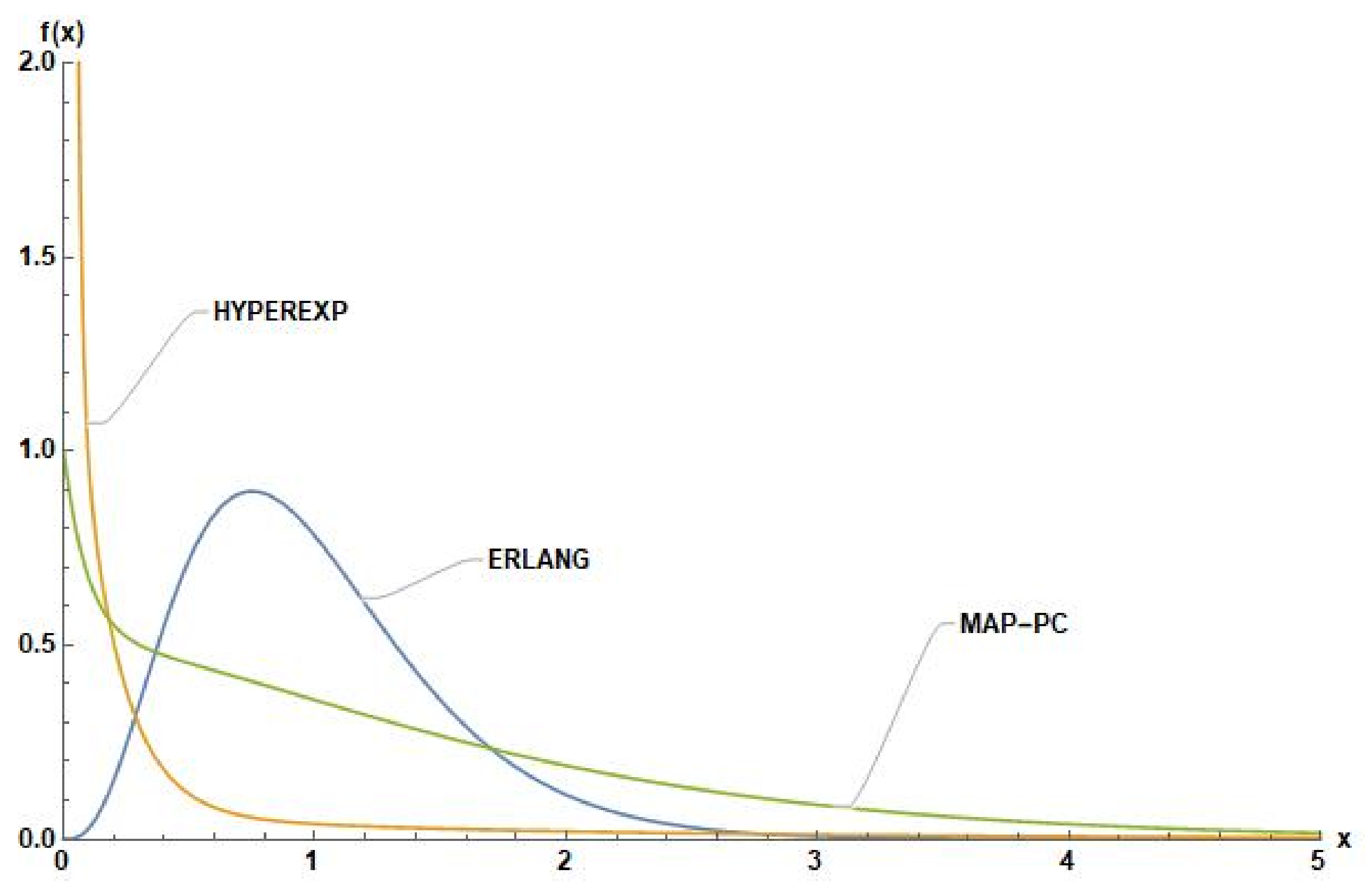
We define the following arrival processes (along with their parameters including the standard deviations):

ERA

Erlang distributed inter-arrival times with density ${\tilde{\lambda }}^k{x}^{k-1}{e}^{-\tilde{\lambda }x}/(k-1)!$, $\tilde{\lambda }=4$, and $k=4$ (standard deviation $\approx 0.5774$).

HEA

Hyperexponential inter-arrival times with density ${\sum }_{i=1}^k{p}_i{\tilde{\lambda }}_i{e}^{-{\tilde{\lambda }}_{i}x}$, $k=4$, ${\tilde{\lambda }}_i=\left(63.1\right)·{10}^{-i},i=1,2,3$, and $p=(0.6,0.25,0.10,0.05)$ (standard deviation $\approx 4.9629$).

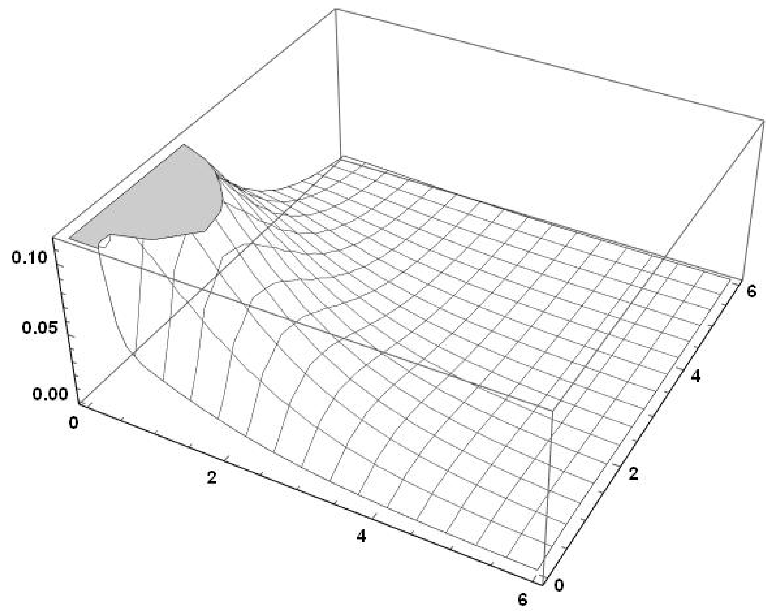
PCA

Markov arrival process $(E_0,E_1)$ with positive correlation $\approx 0.4637$ (standard deviation $\approx 1.3153$), where

$$E_0=\left(\begin{array}{ccc}-1.05& 1.05& 0\\ 0& -1.05& 0\\ 0& 0& -10.5\end{array}\right),E_1=\left(\begin{array}{ccc}0& 0& 0\\ 1.035& 0& 0.0105\\ 0.105& 0& 10.395\end{array}\right).$$

The parameters of distributions are normalized so as to obtain a unit arrival rate. The graphs of the probability density function of the three inter-arrival times are plotted in Figure 1 and the joint probability function of the $MAP$ with positive correlation is plotted in Figure 2.

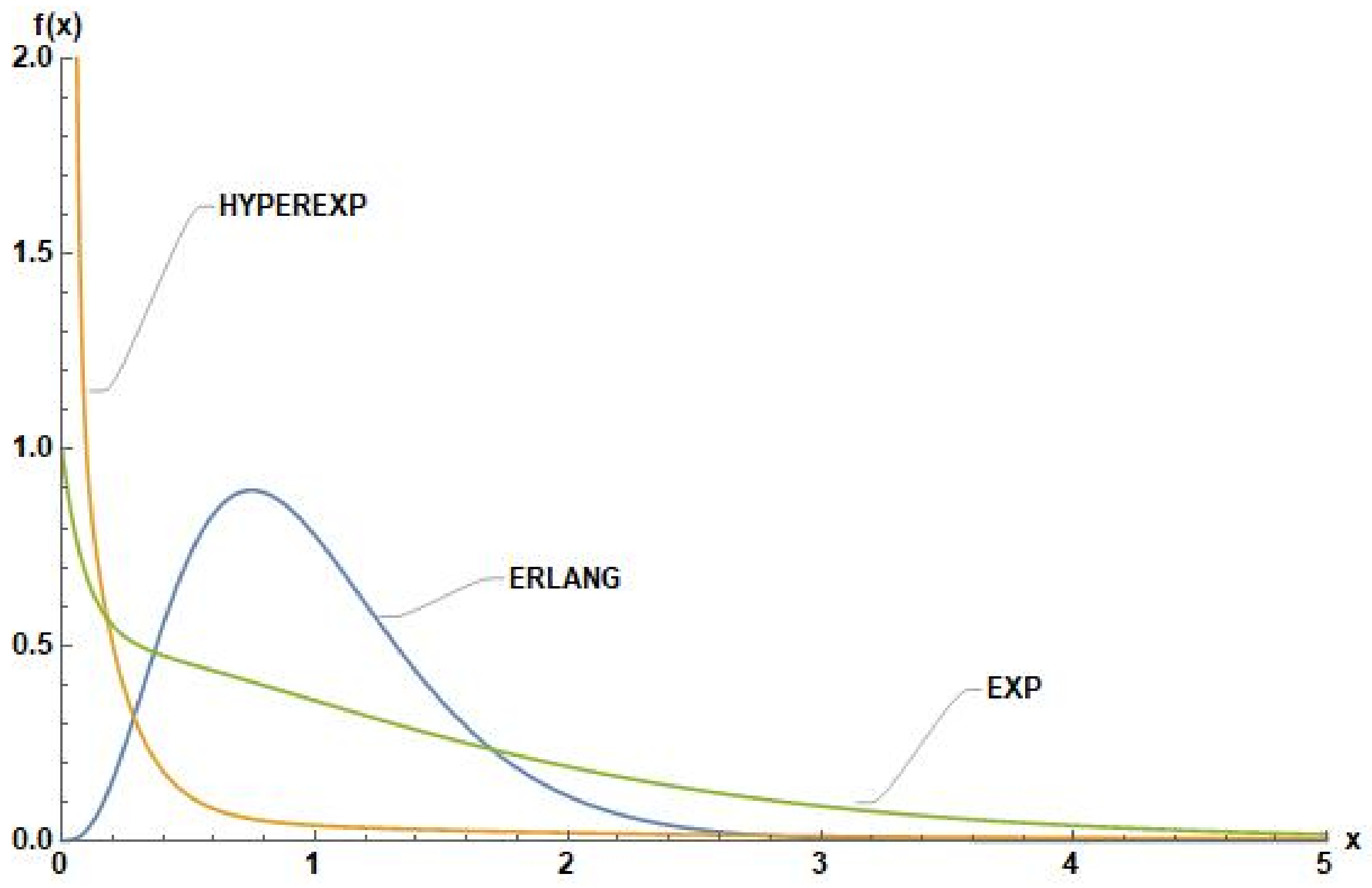
We also use the following service time distributions:

ERS

Erlang distributed service times having density ${\tilde{\mu }}^k{x}^{k-1}{e}^{-\tilde{\mu }x}/(k-1)!$ with $k=3$.

EXS

Exponentially distributed service times of rate $\mu$.

HES

Hyperexponentially distributed service times with density ${\sum }_{i=1}^k{p}_i{\tilde{\mu }}_i{e}^{-{\tilde{\mu }}_{i}x}$, $k=3$, $p=(0.7,0.25,0.05)$ and ${\tilde{\mu }}_i=\left(8.2\mu \right)·{10}^{-i},i=1,\cdots ,3$.

The service rate $\mu$ will be normalized so as to arrive at a given service rate. Obviously, the above three $PH$-distributions are qualitatively different covering a wide range applicable in practice. The plot of these three distributions is given in Figure 3.

For our illustrative examples, here we take the batch size distribution to be uniform in $\{1,\cdots ,N\}$ and the batch size maximum to be N, which is set at $N=7$. It should be pointed out that we did consider other batch size distributions like constant, truncated Poisson, and truncated geometric. For the range of parameters considered, we observed that numerical results with other batch size distribution are similar to those with uniform distribution.

When a replenishment opportunity occurs, an order is placed with probability 1 when the inventory level is at most L, and with probability $a_i$, when the inventory level is $i,L+1<i\le K-1$. Order quantity is always determined to bring the inventory level to K. We considered three types of probability functions for $a_i$, namely, constant, linearly decreasing, and non-linearly decreasing for $i=L+1\le i\le K-1$. We observed that the effect of the type of probability function used for $a_i$ on the system performance is minimal. In many cases, the corresponding results for the three probability functions are equal within the fourth decimal.

Queuing-inventory systems consist of two interacting subsystems, namely the inventory subsystem (ISS) and the customer subsystem (CSS).

• In ISS, inventory is consumed and replenished as needed and is characterized by the parameters $K,L$, $\gamma$ and the distribution of the time between two opportunities for replenishment. The arrival process to CSS impacts ISS through the demand for items. ${\widehat{\mu }}_1[{\widehat{\mu }}_2$], ${\widehat{\sigma }}_1[{\widehat{\sigma }}_2$], ${\Gamma }_1[{\Gamma }_2$], ${\xi }_1[{\xi }_2$], ${\kappa }_1[{\kappa }_2$] represent the measures of performance for ISS for Model 1 [Model 2].
• In CSS, customers arrive, receive service (plus items from inventory), and depart and are characterized by the arrival and service processes. Some arrivals are lost due to lack of inventory at the time of arrival. In Model 2, customers may also be lost at a service completion epoch due to lack of inventory at that moment. Customer loss is impacted by the availability of inventory in ISS. ${\mu }_1\left[{\mu }_2\right]$, ${\sigma }_1\left[{\sigma }_2\right]$, ${\nu }_1\left[{\nu }_2\right]$, ${\nu }_1^{*}\left[{\nu }_2^{*}\right]$, ${\vartheta }_1[{\vartheta }_{2a},{\vartheta }_{2d}]$ represent measures of performance for CSS for Model 1 [Model 2].

Inventory levels control the interaction between the two subsystems. If the inventory levels are high [low], customer loss and the interaction between ISS and CSS will be low [high]. In the limiting case when infinite inventory is maintained, interaction between the two subsystems decreases to zero and Model 2 converges to Model 1. In this paper, we consider ${\vartheta }_1\left[{\vartheta }_2\right]$ and ${\mu }_1\left[{\mu }_2\right]$ as good measures for describing the extent of interaction between ISS and CSS for the two models.

Table 1. Customer subsystem ($\mu$ = 1.1).

					Model 1					Model 2
Arr.	Ser.	$\mathbf{\gamma }$	$\mathit{K}$	$\mathit{L}$	${\mathbf{\mu }}_{\mathbf{1}}$	${\mathbf{\sigma }}_{\mathbf{1}}$	${\mathbf{\nu }}_{\mathbf{1}}$	${\mathbf{\nu }}_{\mathbf{1}}^{*}$	${\mathbf{\vartheta }}_{\mathbf{1}}$	${\mathbf{\mu }}_{\mathbf{2}}$	${\mathbf{\sigma }}_{\mathbf{2}}$	${\mathbf{\nu }}_{\mathbf{2}}$	${\mathbf{\nu }}_{\mathbf{2}}^{*}$	${\mathbf{\vartheta }}_{\mathbf{2}\mathbf{a}}$	${\mathbf{\vartheta }}_{\mathbf{2}\mathbf{d}}$
ERA	ERS	0.05	50	20	0.800	1.243	0.594	0.146	0.553	0.851	1.387	0.605	0.140	0.520	0.046
ERA	ERS	0.05	50	30	0.841	1.284	0.581	0.151	0.539	0.896	1.433	0.591	0.145	0.505	0.045
ERA	ERS	0.05	60	20	0.929	1.362	0.552	0.162	0.507	0.978	1.500	0.564	0.156	0.476	0.044
ERA	ERS	0.05	60	30	0.982	1.412	0.536	0.169	0.490	1.033	1.554	0.548	0.161	0.460	0.043
ERA	ERS	0.1	50	20	1.307	1.536	0.394	0.295	0.333	1.356	1.683	0.414	0.275	0.300	0.056
ERA	ERS	0.1	50	30	1.412	1.618	0.368	0.314	0.305	1.465	1.770	0.388	0.292	0.275	0.052
ERA	ERS	0.1	60	20	1.467	1.657	0.355	0.325	0.290	1.504	1.789	0.377	0.302	0.263	0.051
ERA	ERS	0.1	60	30	1.590	1.754	0.328	0.348	0.261	1.632	1.889	0.349	0.323	0.236	0.048
ERA	HES	0.05	50	20	3.598	7.554	0.594	0.301	0.554	4.493	10.916	0.646	0.282	0.461	0.149
ERA	HES	0.05	50	30	3.899	8.040	0.581	0.310	0.539	4.827	11.457	0.633	0.291	0.447	0.150
ERA	HES	0.05	60	20	4.553	9.000	0.551	0.335	0.506	5.160	11.827	0.613	0.311	0.420	0.154
ERA	HES	0.05	60	30	4.976	9.648	0.536	0.346	0.490	5.580	12.476	0.598	0.321	0.404	0.154
ERA	HES	0.1	50	20	8.942	14.632	0.394	0.522	0.333	6.785	13.328	0.504	0.474	0.263	0.192
ERA	HES	0.1	50	30	10.233	16.246	0.368	0.549	0.305	7.428	14.150	0.483	0.494	0.242	0.189
ERA	HES	0.1	60	20	10.935	17.085	0.355	0.565	0.290	7.590	14.288	0.474	0.509	0.231	0.191
ERA	HES	0.1	60	30	12.650	19.147	0.328	0.596	0.261	8.368	15.260	0.452	0.532	0.210	0.187
HEA	ERS	0.05	50	20	1.854	3.755	0.702	0.591	0.672	4.103	9.868	0.729	0.527	0.368	0.334
HEA	ERS	0.05	50	30	1.940	3.866	0.695	0.597	0.664	4.411	10.366	0.717	0.534	0.355	0.334
HEA	ERS	0.05	60	20	2.433	4.633	0.664	0.618	0.630	4.898	11.088	0.699	0.544	0.337	0.332
HEA	ERS	0.05	60	30	2.560	4.790	0.655	0.627	0.620	5.305	11.715	0.685	0.552	0.323	0.330
HEA	ERS	0.1	50	20	3.140	5.378	0.589	0.811	0.548	6.310	12.724	0.630	0.707	0.202	0.391
HEA	ERS	0.1	50	30	3.363	5.637	0.576	0.821	0.533	7.104	13.825	0.606	0.718	0.186	0.381
HEA	ERS	0.1	60	20	4.135	6.737	0.546	0.836	0.500	7.416	14.206	0.597	0.723	0.179	0.378
HEA	ERS	0.1	60	30	4.469	7.121	0.530	0.848	0.483	8.441	15.577	0.570	0.736	0.162	0.365
HEA	HES	0.05	50	20	2.724	6.166	0.702	0.584	0.672	6.331	17.011	0.738	0.530	0.396	0.315
HEA	HES	0.05	50	30	2.863	6.385	0.695	0.590	0.664	6.756	17.756	0.728	0.536	0.385	0.316
HEA	HES	0.05	60	20	3.608	7.659	0.664	0.611	0.630	7.351	18.528	0.709	0.549	0.361	0.319
HEA	HES	0.05	60	30	3.818	7.975	0.655	0.619	0.620	7.897	19.437	0.697	0.556	0.348	0.318
HEA	HES	0.1	50	20	5.208	10.094	0.589	0.781	0.548	8.912	20.301	0.654	0.702	0.240	0.379
HEA	HES	0.1	50	30	5.610	10.656	0.576	0.790	0.533	9.735	21.506	0.636	0.710	0.226	0.374
HEA	HES	0.1	60	20	6.863	12.535	0.546	0.806	0.501	10.192	21.985	0.623	0.719	0.212	0.374
HEA	HES	0.1	60	30	7.468	13.348	0.530	0.817	0.483	11.226	23.441	0.604	0.729	0.196	0.368
PCA	ERS	0.05	50	20	0.762	2.337	0.673	0.473	0.640	2.372	12.737	0.682	0.462	0.419	0.230
PCA	ERS	0.05	50	30	0.798	2.407	0.660	0.498	0.626	2.641	13.843	0.669	0.486	0.396	0.239
PCA	ERS	0.05	60	20	0.978	3.094	0.645	0.517	0.610	3.020	15.335	0.658	0.503	0.375	0.248
PCA	ERS	0.05	60	30	1.028	3.195	0.632	0.546	0.595	3.408	16.816	0.643	0.531	0.349	0.257
PCA	ERS	0.1	50	20	1.553	4.613	0.553	0.727	0.508	4.362	19.515	0.574	0.701	0.218	0.311
PCA	ERS	0.1	50	30	1.654	4.825	0.537	0.768	0.490	5.186	22.225	0.555	0.740	0.188	0.320
PCA	ERS	0.1	60	20	2.092	6.237	0.529	0.765	0.481	5.427	23.006	0.555	0.736	0.187	0.321
PCA	ERS	0.1	60	30	2.238	6.543	0.513	0.806	0.464	6.573	26.474	0.536	0.774	0.158	0.328
PCA	HES	0.05	50	20	2.132	5.285	0.673	0.525	0.640	5.142	22.448	0.701	0.496	0.432	0.239
PCA	HES	0.05	50	30	2.290	5.552	0.660	0.549	0.626	5.574	23.685	0.688	0.516	0.413	0.244
PCA	HES	0.05	60	20	2.616	6.316	0.645	0.568	0.610	6.030	24.915	0.678	0.534	0.390	0.256
PCA	HES	0.05	60	30	2.811	6.634	0.632	0.594	0.595	6.589	26.449	0.664	0.556	0.369	0.261
PCA	HES	0.1	50	20	4.248	9.239	0.553	0.762	0.508	7.712	28.419	0.607	0.712	0.254	0.314
PCA	HES	0.1	50	30	4.606	9.777	0.537	0.797	0.490	8.545	30.479	0.590	0.742	0.230	0.319
PCA	HES	0.1	60	20	5.195	11.193	0.529	0.796	0.481	8.870	31.287	0.588	0.742	0.222	0.325
PCA	HES	0.1	60	30	5.625	11.838	0.513	0.830	0.464	9.930	33.825	0.571	0.772	0.199	0.329

and

Table 2. Inventory subsystem—$\mu$ = 1.1, ERS.

				Model 1					Model 2
Arr.	$\mathbf{\gamma }$	$\mathit{K}$	$\mathit{L}$	${\widehat{\mathbf{\mu }}}_{\mathbf{1}}$	${\widehat{\mathbf{\sigma }}}_{\mathbf{1}}$	${\Gamma }_{\mathbf{1}}$	${\mathbf{\xi }}_{\mathbf{1}}$	${\mathbf{\kappa }}_{\mathbf{1}}$	${\widehat{\mathbf{\mu }}}_{\mathbf{2}}$	${\widehat{\mathbf{\sigma }}}_{\mathbf{2}}$	${\Gamma }_{\mathbf{2}}$	${\mathbf{\xi }}_{\mathbf{2}}$	${\mathbf{\kappa }}_{\mathbf{2}}$
ERA	0.05	50	20	11.692	16.321	47.055	0.735	27.228	12.398	16.642	46.897	0.718	27.861
ERA	0.05	50	30	12.410	16.727	44.536	0.804	24.878	13.155	17.034	44.260	0.789	25.342
ERA	0.05	60	20	15.421	19.918	56.746	0.677	29.537	16.253	20.247	56.578	0.660	30.296
ERA	0.05	60	30	16.403	20.333	54.240	0.735	27.215	17.223	20.632	54.003	0.720	27.791
ERA	0.10	50	20	18.142	17.416	44.610	0.583	17.158	18.849	17.486	44.379	0.566	17.678
ERA	0.10	50	30	19.864	17.752	40.356	0.673	14.855	20.583	17.778	40.015	0.658	15.206
ERA	0.10	60	20	22.995	20.644	54.013	0.515	19.433	23.727	20.715	53.788	0.500	20.003
ERA	0.10	60	30	25.101	20.820	49.822	0.583	17.155	25.839	20.818	49.509	0.569	17.592
HEA	0.05	50	20	22.059	22.423	47.842	0.529	37.781	23.096	21.213	46.314	0.499	40.081
HEA	0.05	50	30	22.786	22.726	46.149	0.563	35.502	23.943	21.331	43.373	0.557	35.894
HEA	0.05	60	20	26.855	26.413	57.532	0.499	40.049	28.058	24.908	55.905	0.462	43.287
HEA	0.05	60	30	27.820	26.714	55.848	0.529	37.782	29.090	24.932	53.056	0.511	39.182
HEA	0.10	50	20	28.909	21.539	46.540	0.376	26.572	28.910	19.603	43.757	0.363	27.541
HEA	0.10	50	30	30.178	21.720	44.134	0.410	24.368	30.311	19.383	39.322	0.431	23.199
HEA	0.10	60	20	34.649	25.150	55.954	0.348	28.752	34.484	22.873	52.992	0.328	30.487
HEA	0.10	60	30	36.260	25.219	53.575	0.376	26.573	36.080	22.419	48.708	0.382	26.208
PCA	0.05	50	20	16.747	17.684	45.521	0.615	32.508	17.322	17.644	45.190	0.603	33.193
PCA	0.05	50	30	18.184	18.117	41.838	0.697	28.701	18.788	18.022	41.335	0.688	29.058
PCA	0.05	60	20	21.269	21.103	55.111	0.553	36.149	21.979	21.000	54.703	0.539	37.141
PCA	0.05	60	30	23.030	21.436	51.562	0.615	32.510	23.778	21.255	50.943	0.604	33.102
PCA	0.10	50	20	23.346	17.188	42.458	0.454	22.055	23.965	16.855	41.808	0.440	22.751
PCA	0.10	50	30	25.980	17.206	36.985	0.541	18.480	26.618	16.736	36.101	0.534	18.762
PCA	0.10	60	20	28.547	20.167	51.733	0.394	25.408	29.262	19.730	50.926	0.379	26.462
PCA	0.10	60	30	31.492	19.905	46.540	0.454	22.055	32.211	19.311	45.446	0.444	22.564

respectively summarize the results for CSS and ISS for a broad range of parameter values. These tables represent a subset of the numerical results used in the following qualitative summary of the effect of various parameters on the performance of two subsystems for the two models.

Table 3. Comparing Model 1 and Model 2

Model 1 ($\mathit{\mu }$ = 1.1, $\mathit{\gamma }$ = 0.1, K = 50)
Arr.	Ser.	$\mathit{L}$	${\mathbf{\mu }}_{\mathbf{1}}$	${\mathbf{\sigma }}_{\mathbf{1}}$	${\widehat{\mathbf{\mu }}}_{\mathbf{1}}$	${\widehat{\mathbf{\sigma }}}_{\mathbf{1}}$	${\Gamma }_{\mathbf{1}}$	${\mathbf{\kappa }}_{\mathbf{1}}$	${\mathbf{\nu }}_{\mathbf{1}}$	${\mathbf{\nu }}_{\mathbf{1}}^{*}$	${\mathbf{\vartheta }}_{\mathbf{1}}$	${\mathbf{\vartheta }}_{\mathbf{1}}^{*}$
ERA	ERS	20	1.307	1.536	18.142	17.416	44.610	17.158	0.394	0.295	0.333	0.000
ERA	ERS	30	1.412	1.618	19.864	17.752	40.356	14.855	0.368	0.314	0.305	0.000
ERA	EXS	20	1.844	2.391	18.143	17.415	44.609	17.158	0.394	0.345	0.333	0.000
ERA	EXS	30	2.023	2.566	19.867	17.751	40.353	14.855	0.368	0.366	0.305	0.000
ERA	HES	20	8.942	14.632	18.141	17.415	44.608	17.165	0.394	0.522	0.333	0.000
ERA	HES	30	10.233	16.246	19.865	17.750	40.348	14.861	0.368	0.549	0.305	0.000
HEA	ERS	20	3.140	5.378	28.909	21.539	46.540	26.572	0.589	0.811	0.548	0.000
HEA	ERS	30	3.363	5.637	30.178	21.720	44.134	24.368	0.576	0.821	0.533	0.000
HEA	EXS	20	3.244	5.605	28.909	21.539	46.540	26.570	0.589	0.809	0.548	0.000
HEA	EXS	30	3.476	5.878	30.178	21.720	44.134	24.366	0.576	0.819	0.533	0.000
HEA	HES	20	5.208	10.094	28.909	21.539	46.540	26.573	0.589	0.781	0.548	0.000
HEA	HES	30	5.610	10.656	30.177	21.720	44.134	24.367	0.576	0.790	0.533	0.000
PCA	ERS	20	1.553	4.613	23.346	17.188	42.458	22.055	0.553	0.727	0.508	0.000
PCA	ERS	30	1.654	4.825	25.980	17.206	36.985	18.480	0.537	0.768	0.490	0.000
PCA	EXS	20	1.681	4.771	23.345	17.190	42.460	22.050	0.553	0.732	0.508	0.000
PCA	EXS	30	1.793	4.991	25.982	17.205	36.983	18.479	0.537	0.772	0.490	0.000
PCA	HES	20	4.248	9.239	23.345	17.189	42.458	22.055	0.553	0.762	0.508	0.000
PCA	HES	30	4.606	9.777	25.978	17.207	36.987	18.480	0.537	0.797	0.490	0.000
ERA	ERS	20	1.356	1.683	18.849	17.486	44.379	17.678	0.414	0.275	0.356	0.156
ERA	ERS	30	1.465	1.770	20.583	17.778	40.015	15.206	0.388	0.292	0.327	0.160
ERA	EXS	20	1.916	2.678	19.334	17.625	44.312	18.046	0.428	0.314	0.371	0.210
ERA	EXS	30	2.101	2.860	21.112	17.925	39.932	15.509	0.402	0.332	0.342	0.217
ERA	HES	20	6.785	13.328	22.408	18.541	44.228	20.777	0.504	0.474	0.454	0.422
ERA	HES	30	7.428	14.150	24.551	19.020	40.071	18.015	0.483	0.494	0.431	0.439
HEA	ERS	20	6.310	12.724	28.910	19.603	43.757	27.541	0.630	0.707	0.593	0.659
HEA	ERS	30	7.104	13.825	30.311	19.383	39.322	23.199	0.606	0.718	0.567	0.673
HEA	EXS	20	6.480	13.190	29.025	19.635	43.826	27.733	0.632	0.706	0.595	0.654
HEA	EXS	30	7.280	14.306	30.446	19.437	39.457	23.427	0.609	0.717	0.570	0.668
HEA	HES	20	8.912	20.301	30.279	19.907	44.550	30.039	0.654	0.702	0.619	0.612
HEA	HES	30	9.735	21.506	31.912	19.896	40.902	26.200	0.636	0.710	0.600	0.624
PCA	ERS	20	4.362	19.515	23.965	16.855	41.808	22.751	0.574	0.701	0.529	0.587
PCA	ERS	30	5.186	22.225	26.618	16.736	36.101	18.762	0.555	0.740	0.509	0.630
PCA	EXS	20	4.568	20.087	24.067	16.891	41.823	22.856	0.576	0.702	0.533	0.584
PCA	EXS	30	5.392	22.750	26.719	16.774	36.134	18.851	0.557	0.740	0.512	0.625
PCA	HES	20	7.712	28.419	25.607	17.460	42.148	24.912	0.607	0.712	0.568	0.552
PCA	HES	30	8.545	30.479	28.307	17.489	36.858	20.822	0.590	0.742	0.549	0.581

compares the system measures for the two models. In these tables, the abbreviations Arr. and Ser. are used to identify the arrival process and service time distribution.

5.1. Impact of Service Rate and Service Time Distribution

In Model 1, customers do not enter the system when inventory level is zero, and when a customer enters the system the inventory level is immediately reduced to reflect the new customer’s demand. As a consequence, the service rate and service time distribution do not impact ISS. They do impact ISS in Model 2 because customers who arrive when inventory level is zero wait in line hoping for a replenishment during their wait. However, this impact is minimal because the likelihood of a replenishment during their wait is typically very small.

As it might be expected, the performance measures for CSS improved with increasing service rate in both models. The overall impact of service time variability is to degrade the performance of the system, with HES generating the strongest impact. Specifically, increasing service rate increased the probability of an idle server (${\nu }_1,{\nu }_2$) and decreased the number of customers in the system (${\mu }_1,{\mu }_2$). Increasing variability of service time distribution, on the other hand, increased the mean (${\mu }_1,{\mu }_2$), the standard deviation (${\sigma }_1,{\sigma }_2$), and the coefficient of variation of the number of customers in the system, and increased the percent of time the server is idle with positive inventory (${\nu }_1^{*},{\nu }_2^{*})$. The probability of customer loss in Model 1 (${\nu }_1$) was unaffected by the service time variability, but ${\nu }_2$ increased marginally. We also observed that when the service rate is less than the arrival rate, ${\nu }_1<{\vartheta }_1$ and ${\nu }_2<{\vartheta }_2$; and when service rate is greater than the arrival rate, ${\nu }_1>{\vartheta }_1$ and ${\nu }_2>{\vartheta }_2$.

5.2. Effect of Arrival Process

Arrival process impacts both the ISS and the CSS and in general, increasing variability of arrivals had the effect of degrading the performance of the system. It is interesting to note that for systems with both a highly variable arrival process and service time distribution, the combined effect is more attenuated than the individual effects.

Systems with highly variable arrival processes (HEA and PCA relative to ERA) had higher probability of a customer loss (${\vartheta }_1$ and ${\vartheta }_2$), and higher mean (${\mu }_1,{\mu }_2$), standard deviation (${\sigma }_1,{\sigma }_2$), and the coefficient of variation of the number of customers in the system. Similarly, HEA and PCA produced higher mean (${\widehat{\mu }}_1,{\widehat{\mu }}_2$), standard deviation (${\widehat{\sigma }}_1,{\widehat{\sigma }}_2$) but lower coefficient of variation of the inventory levels. Mean cycle times (${\xi }_1,{\xi }_2$) were lower but the order quantities (${\Gamma }_1,{\Gamma }_2$) remained relatively unaffected. HEA and PCA increased the probability that the server is idle (${\nu }_1,{\nu }_2$) as well as the percent of time the server is idle with inventory of units on hand (${\nu }_1^{*},{\nu }_2^{*}$), significantly degrading the system performance. The impact of HEA was more pronounced than PCA.

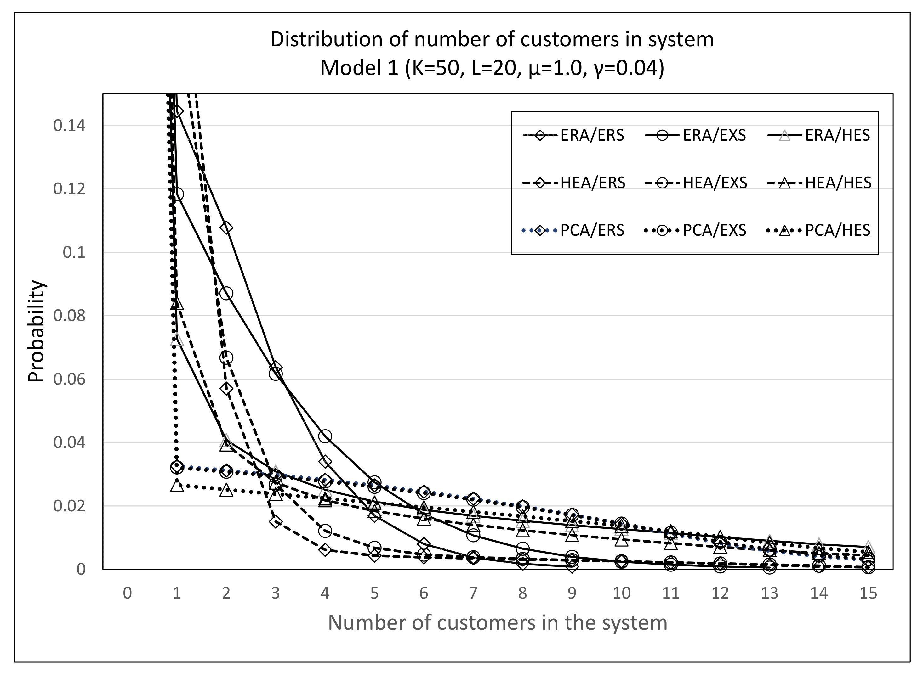
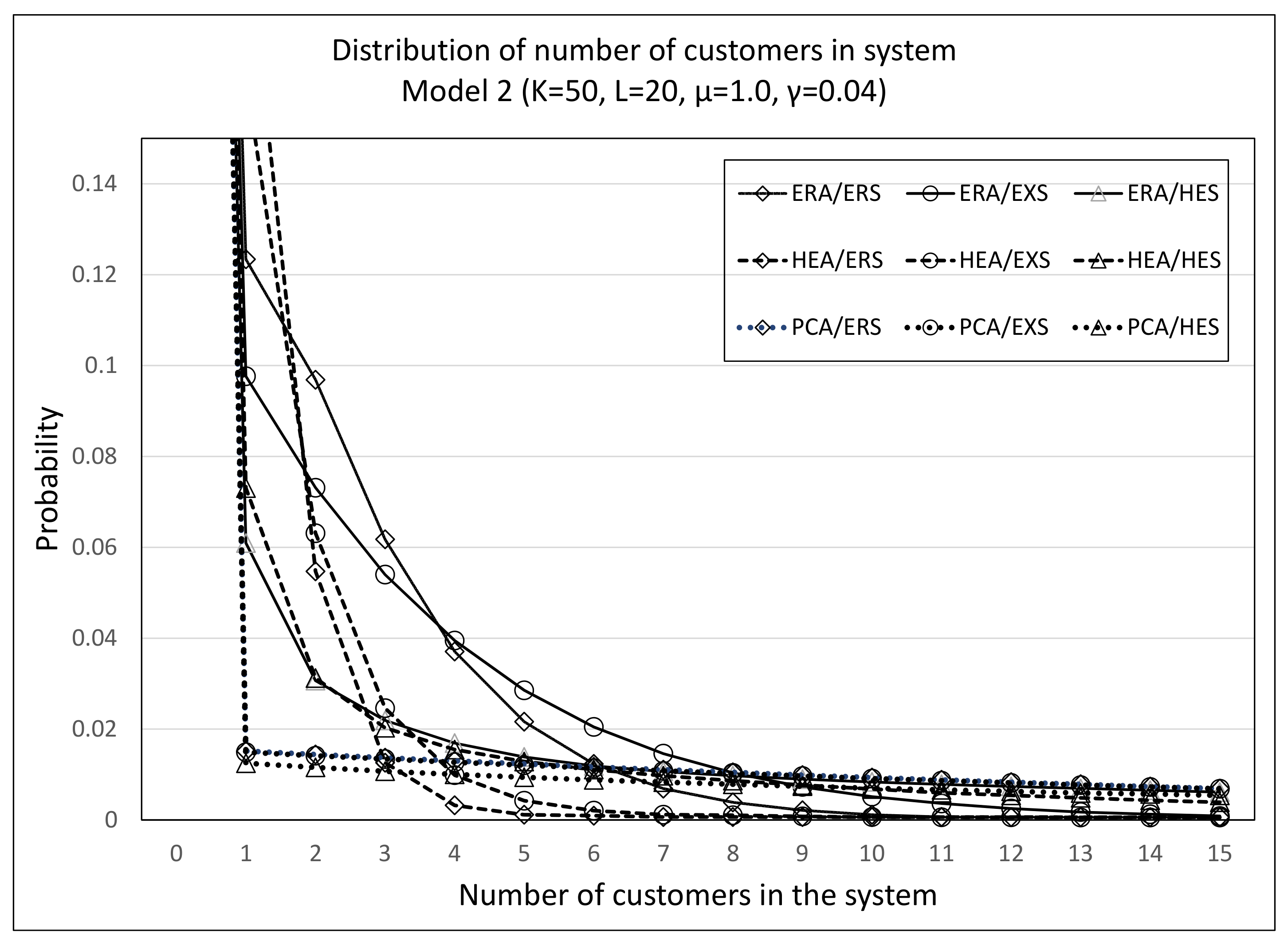
Figure 4 and Figure 5 summarize the effect of the arrival and service processes on the steady-state marginal distributions of the number of customers in the system. In these figures, X and Y axes are truncated at much smaller values than required by the results in order to highlight the differences in the probability distributions.

Figure 4 and Figure 5 indicate that increasing variability in the system (either for service times or for the arrival process) shifts the probability from states with smaller number in the system to the states with higher number in the system, thus creating a longer tail for the distribution. Model 2, in general, has a slightly longer tail relative to Model 1.

5.3. Impact of $\gamma$

$\gamma$ is not under the control of the management but understanding its effect on the system is essential to choose K and L efficient operation of the system. We considered values of $\gamma$ =1/10, 1/15, 1/20, and 1/25 (with $\lambda =1$) in the numerical analysis.

For a given K and L, larger values of $\gamma$ resulted in more frequent usage of opportunistic events to procure replenishment or smaller order cycle times, ${\kappa }_1$ and ${\kappa }_2$), and hence smaller size replenishments, ${\Gamma }_1$ and ${\Gamma }_2$, resulting in a net increase in the mean inventory levels ${\widehat{\mu }}_1$ and ${\widehat{\mu }}_2$). This observation should be interpreted with caution because it states the effect of larger $\gamma$, keeping K and L at the same level. Larger $\gamma$ indicates more frequent opportunities for replenishment permitting smaller K and L to achieve the same service level. Larger $\gamma$, in addition to increasing the means, ${\widehat{\mu }}_1$ and ${\widehat{\mu }}_2$, also increased the standard deviations, ${\widehat{\sigma }}_1$ and ${\widehat{\sigma }}_2$, but with a net decrease in the coefficients of variation of the inventory levels. Larger $\gamma$ also had a similar effect on the numbers of customers in the system by increasing the means, ${\mu }_1$ and ${\mu }_2$, and the standard deviations, ${\sigma }_1$ and ${\sigma }_2$, but resulted in a net decrease in the coefficients of variation. Further discussion on the combined effect of changes in $\gamma$ with other parameters such as K and L is presented in the following.

Inventory system with larger values of $\gamma$, indicating frequent replenishment opportunities, will permit maintaining smaller inventories to achieve the same level of service.

5.4. Impact of K and L

In the inventory subsystem, as K increases, with all other parameters remaining the same, more items are procured when opportunistic events occur leading to larger inventories on average. Larger inventories lead to larger cycle times (${\kappa }_1$ and ${\kappa }_2$) because of an increased likelihood of skipping current opportunities to wait for future ones. The net effect is an increase in the means ${\widehat{\mu }}_1$ and ${\widehat{\mu }}_2$ and also an increase in the standard deviations ${\widehat{\sigma }}_1$ and ${\widehat{\sigma }}_2$, but a reduction in the coefficient of variation of the inventory levels. Changes in L had a slightly different, and smaller, effect on the inventory subsystem than corresponding changes in K. As L increases with all other parameters remaining the same, opportunistic events are availed more often (smaller ${\kappa }_1$ and ${\kappa }_2$) and in smaller quantities. The net result is once again an increase in the means, ${\widehat{\mu }}_1$ and ${\widehat{\mu }}_2$, and an increase in the standard deviations, ${\widehat{\sigma }}_1$ and ${\widehat{\sigma }}_2$), but a reduction in the coefficient of variation, of the numbers in the system.

In the customer subsystem, increasing K or L keeping the rest of the parameters the same, led to an increase in the means, ${\mu }_1$ and ${\mu }_2$, and an increase in the standard deviations, ${\sigma }_1$ and ${\sigma }_2$, but a reduction in the coefficient of variation, of the number of customers in the system. Increasing K or L also resulted in a decrease the customer loss probability (${\vartheta }_1,{\vartheta }_2)$, server idle probability (${\nu }_1,{\nu }_2$), and an increase in the percent of server idle time with positive inventory (${\nu }_1^{*},{\nu }_2^{*}$). Effect of changes in K are much stronger than corresponding changes in L.

5.5. Cost Analysis

A system that can provide the desired service level at the minimum cost is the goal of any optimization. We consider three costs associated with the system, namely, cost of carrying inventory, cost of placing an order, and cost of lost customers/demand. A fourth item, the cost of keeping customers waiting, is not considered in this study because it was not considered particularly relevant. Let $c_1$, $c_2$, and $c_3$ denote the costs of carrying a unit inventory per unit time, cost of placing an order, and the average cost of a lost customer. $Z_1$ and $Z_2$, the total cost per unit time for the two models can be expressed as follows. The system cost per unit time is then given by

$$\begin{array}{ccc}\hfill Z_1\hfill & =& c_1{\widehat{\mu }}_1+\frac{c_2}{{\kappa }_1}+c_3{\vartheta }_1\hfill \\ \hfill Z_2\hfill & =& c_1{\widehat{\mu }}_2+\frac{c_2}{{\kappa }_2}+c_3({\vartheta }_{2a}+{\vartheta }_{2d})\hfill \end{array}$$

The first two components in $Z_1$ and $Z_2$ represent the cost of the inventory subsystem, and the third item represents the cost of the customer subsystem. The goal of management is to choose the values of K and L that minimize the total cost. Using values of $c_1$ = 0.25, $c_2$ = 100, and $c_3$ = 10, a summary of the cost for a select set of parameter values is presented in

Table 4. Total cost summary $\gamma$ = 0.1, $\mu$ = 1.1.

Service Dist.		ERS			EXS			HES
Arr.	$\mathit{L}/\mathit{K}$	40	50	60	40	50	60	40	50	60
Model 1
ERA	10	13.085	12.946	13.125	13.084	12.942	13.123	13.080	12.941	13.123
ERA	20	13.982	13.695	13.799	13.981	13.695	13.797	13.979	13.691	13.796
ERA	30	15.304	14.751	14.718	15.303	14.750	14.717	15.301	14.745	14.708
HEA	10	15.453	15.999	16.667	15.453	16.000	16.669	15.453	16.000	16.668
HEA	20	15.925	16.470	17.145	15.926	16.471	17.146	15.926	16.470	17.146
HEA	30	16.444	16.982	17.662	16.445	16.983	17.663	16.444	16.983	17.663
PCA	10	14.161	14.445	14.976	14.164	14.446	14.981	14.162	14.444	14.979
PCA	20	15.355	15.448	15.886	15.356	15.451	15.888	15.355	15.449	15.885
PCA	30	17.125	16.807	17.046	17.127	16.810	17.050	17.125	16.808	17.047
Model 2
ERA	10	13.258	13.184	13.412	13.363	13.333	13.598	13.913	14.120	14.596
ERA	20	14.169	13.928	14.077	14.281	14.084	14.260	14.871	14.957	15.364
ERA	30	15.541	14.993	14.979	15.656	15.144	15.161	16.158	16.000	16.289
HEA	10	15.622	16.262	17.034	15.635	16.283	17.062	15.778	16.507	17.358
HEA	20	16.280	16.786	17.465	16.292	16.812	17.502	16.423	17.089	17.901
HEA	30	17.263	17.557	18.106	17.258	17.577	18.143	17.229	17.795	18.550
PCA	10	14.306	14.664	15.277	14.333	14.703	15.323	14.618	15.096	15.803
PCA	20	15.533	15.681	16.174	15.556	15.720	16.228	15.787	16.093	16.710
PCA	30	17.360	17.072	17.347	17.375	17.107	17.401	17.428	17.373	17.817

, where the minimum cost values for each combination of K and L are highlighted in bold. In order to find the best combination of values of K and L, a more refined search than in Table 4 needs to be performed.

5.6. Comparing Model 1 and Model 2

Table 3 compares the steady behavior of the system under the two models. For a given set of parameter values, Model 1 performed better than Model 2 in terms of the mean number of customers in the system, mean inventory level, and probability of an idle server. For Model 2, the loss of demand can occur either at arrival, or at service completion epochs. ${\vartheta }_2$ is always larger than ${\vartheta }_1$, but the difference is significantly higher for the case of HES. This high loss rate may cause higher idle probability. Higher variability of the arrival process (as in the case of HEA or PSA) appears to mitigate the effect. For Model 2, the proportion of customers lost at departure instants varied from a low of 9.01% to a high of 68.4%. We notice that these percentages are significantly larger for HES, HEA, and PCA.

5.7. Comparing $(K,L)$ System with $(s,S)$ System

In this subsection, we compare the characteristics of the system considered in this paper (the $(K,L)$ system) with the $(s,S)$ system considered in Chakravarthy and Rumyantsev [17]. In the $(K,L)$ system, the replenishment opportunities occur randomly at exponentially distributed intervals with no lead time for delivery. In the $(s,S)$ system in [17], orders are placed as inventory is depleted but the items are received after an exponentially distributed lead time. In other words, the random lead time in the $(s,S)$ system is replaced by the random interval between replenishment opportunities in the $(K-L)$ system. For effective comparison, we use exactly the same parameters for both systems and set $K=S$ and $L=s$, and the mean lead time for delivery in the $(s,S)$ system equal to the mean time between two replenishment opportunities in the $(K,L)$ system.

Table 5. Comparing the $(K,L)$ system with the $(s,S)$ system.

		$(\mathit{K},\mathit{L})$ System ($\mathit{\gamma }$ = 0.1, $\mathit{\mu }$ = 1.1, K = 60, L = 20)							$(\mathit{s},\mathit{S})$ System ($\mathit{\gamma }$ = 0.1, $\mathit{\mu }$ = 1.1, S = 60, s = 20)
Model 1
Arr.	Ser.	${\mathbf{\vartheta }}_{\mathbf{1}}$	${\mathbf{\nu }}_{\mathbf{1}}$	${\mathbf{\mu }}_{\mathbf{1}}$	${\mathbf{\sigma }}_{\mathbf{1}}$	${\widehat{\mathbf{\mu }}}_{\mathbf{1}}$	${\widehat{\mathbf{\sigma }}}_{\mathbf{1}}$	${\mathbf{\kappa }}_{\mathbf{1}}$	${\mathbf{\vartheta }}_{\mathbf{1}}$	${\mathbf{\nu }}_{\mathbf{1}}$	${\mathbf{\mu }}_{\mathbf{2}}$	${\mathbf{\sigma }}_{\mathbf{2}}$	${\mathbf{\mu }}_{\mathbf{2}}$	${\widehat{\mathbf{\sigma }}}_{\mathbf{2}}$	${\mathbf{\kappa }}_{\mathbf{1}}$
ERA	ERS	0.355	0.290	1.467	1.657	22.995	20.644	19.433	0.423	0.365	1.209	1.475	15.660	16.179	16.221
ERA	EXS	0.355	0.290	2.116	2.644	22.999	20.642	19.439	0.423	0.365	1.686	2.267	15.663	16.178	16.222
ERA	HES	0.355	0.290	10.935	17.085	22.986	20.646	19.437	0.423	0.365	7.784	13.214	15.657	16.179	16.223
HEA	ERS	0.546	0.500	4.135	6.737	34.649	25.150	28.752	0.629	0.592	2.438	4.414	24.481	19.098	25.437
HEA	EXS	0.546	0.501	4.272	7.014	34.650	25.149	28.749	0.629	0.592	2.520	4.601	24.481	19.098	25.436
HEA	HES	0.546	0.501	6.863	12.535	34.649	25.150	28.751	0.629	0.592	4.018	8.259	24.481	19.098	25.437
PCA	ERS	0.529	0.481	2.092	6.237	28.547	20.167	25.408	0.568	0.525	1.220	3.468	21.748	16.972	21.571
PCA	EXS	0.529	0.482	2.239	6.409	28.550	20.163	25.411	0.568	0.525	1.338	3.620	21.749	16.970	21.571
PCA	HES	0.529	0.481	5.195	11.193	28.547	20.163	25.415	0.568	0.525	3.677	7.968	21.747	16.972	21.572
Model 2
Arr.	Ser.	${\mathbf{\vartheta }}_{\mathbf{2}}$	${\mathbf{\nu }}_{\mathbf{2}}$	${\mathbf{\mu }}_{\mathbf{2}}$	${\mathbf{\sigma }}_{\mathbf{2}}$	${\widehat{\mathbf{\mu }}}_{\mathbf{2}}$	${\widehat{\mathbf{\sigma }}}_{\mathbf{2}}$	${\mathbf{\kappa }}_{\mathbf{2}}$	${\mathbf{\vartheta }}_{\mathbf{2}}$	${\mathbf{\nu }}_{\mathbf{2}}$	${\mathbf{\mu }}_{\mathbf{2}}$	${\mathbf{\sigma }}_{\mathbf{2}}$	${\mathbf{\mu }}_{\mathbf{2}}$	${\widehat{\mathbf{\sigma }}}_{\mathbf{2}}$	${\mathbf{\kappa }}_{\mathbf{2}}$
ERA	ERS	0.377	0.315	1.504	1.789	23.727	20.715	20.003	0.441	0.385	1.271	1.637	16.357	16.730	16.748
ERA	EXS	0.391	0.330	2.151	2.883	24.273	20.838	20.445	0.453	0.398	1.796	2.600	16.843	16.946	17.113
ERA	HES	0.474	0.421	7.590	14.288	27.673	21.708	23.619	0.524	0.476	6.418	12.959	19.846	18.270	19.642
HEA	ERS	0.597	0.556	7.416	14.206	34.484	22.873	30.487	0.651	0.616	5.766	12.099	25.218	18.109	26.769
HEA	EXS	0.599	0.559	7.594	14.674	34.623	22.909	30.690	0.653	0.618	5.931	12.567	25.307	18.153	26.928
HEA	HES	0.623	0.586	10.192	21.985	36.118	23.210	33.174	0.675	0.643	8.199	19.488	26.326	18.629	28.909
PCA	ERS	0.555	0.508	5.427	23.006	29.262	19.730	26.462	0.583	0.540	4.024	18.494	22.363	17.226	22.283
PCA	EXS	0.557	0.512	5.641	23.527	29.380	19.768	26.565	0.585	0.543	4.220	19.058	22.436	17.207	22.384
PCA	HES	0.588	0.547	8.870	31.287	31.069	20.387	28.799	0.617	0.578	7.246	27.332	23.755	17.800	24.279

presents a summary comparison for $\gamma$ = 0.1, $\mu$ = 1.1, $K=S=60$, $L=s=20$ for both Model 1 and Model 2, for all arrival and service distributions considered in Section 3.

The summary indicates that for the combinations of parameters considered, $(K,L)$ system has a smaller server idle probability, smaller customer loss probability but on all other counts $(s,S)$ system had better operational performance for both Model 1 and Model 2. Considering the customer subsystem, $(K,L)$ model has larger mean and standard deviation of the number of customers in the system relative to the $(s,S)$ system. In the inventory subsystem, $(K,L)$ model has a larger cycle time, and a larger mean and standard deviation of the inventory level relative to the $(s,S)$ system. This indicates that orders are placed less often in the $(K,L)$ system, and more units are ordered each time an order is placed, resulting in larger mean inventory level with greater variability. The overall conclusion from these observations is that the additional uncertainty introduced in the system by the random supply process adversely affects the system performance.

Cost computations are not performed because the results depend significantly on the relative values of $c_1$, $c_2$, and $c_3$. Furthermore, direct comparison of total costs could be misleading because one has to optimize the two systems separately and then compare the two optimal solutions to see which performs better. Even that is not very meaningful, because one does not choose between a $(K,L)$ system or an $(s,S)$ system.

6. Concluding Remarks

In this paper, we considered a queuing-inventory system where the replenishment opportunities occur at random intervals at which time the decisions are made with regard to the procurement and the quantities. We proposed an opportunistic system involving two parameters, L and K, similar to the well-known $(s,S)$ inventory management system. The cut-off point, L, between 0 and K, largely determines whether to avail the opportunistic replenishment with certainty or with a probabilistic rule. The two models considered differ in the way the customers enter the system or are getting lost. In Model 1, the customers are lost when the inventory level is zero (irrespective of whether the server is idle or busy). In Model 2, the customers are allowed to enter even when the inventory level is zero but as long as the server is busy serving. Further, the customers may be lost at a service completion due to lack of inventory to start a new service.

The analysis of the results from an extensive set of numerical experimentation under various scenarios of the parameters indicates that with all other parameters remaining the same, Model 1 appears to have better performance characteristics in terms of the number of customers in the system, inventory levels in the system, and the likelihood of losing a customer.

Variability in the overall system behavior can be due to the variability in the arrival process or the service time distribution. In general, increasing the variability of either the input process or the service time distribution, led to an increase in overall variability in the system behavior. When both arrival process and service time distribution are highly variable, the combined effect is more attenuated than the individual effects.

With the tools developed in this paper and the understanding of the system behavior presented in this paper, it is possible to conduct an efficient search for the value of the key parameters K, and L that minimizes the total system cost. While $\gamma$, the rate at which replenishment opportunities arise, is not under the control of the management, one might surmise that an optimal inventory system with larger values of $\gamma$ will have smaller cost because of the availability of frequent replenishment opportunities making it possible to achieve the same level of service with smaller inventories.

A comparison with the $(s,S)$ system studied by Chakravarthy and Rumyantsev [17] revealed that, the $(s,S)$ system has better operating characteristics in terms of number in the system and inventory levels, apparently due to the random supply process. This could be mitigated by the possibly having a lower purchase cost per unit. This aspect is not studied in this paper. In addition, it would be interesting to compare the system studied here with the $(s,S)$ system in which the inventory level is always brought to level S, irrespective of when the replenishment occurs.

A possible extension to this study could be to investigate systems with both regular channels of purchase (as in the $(s,S)$ system) and the opportunistic replenishment opportunities (as in the $(K,L)$ system) with possibly lower per unit cost of purchase in the context of $MAP$ arrivals of demands and phase-type services.

In this paper, we explored two queuing-inventory models where the replenishment opportunities occur at random. Such models are appropriate for non-critical items (e.g., canned goods, generic medication) where stock outs for short periods of time are not serious. Special replenishment opportunities typically offer lower unit cost with little or no ordering cost, and units are usually available without delay. The results of this paper and the detailed discussion of the system behavior, offer a useful tool to compare the traditional inventory systems (e.g., $(s,S)$ system) with the opportunistic models to determine the most effective method to manage inventories under a more general scenario of using $MAP$ for the demand process and phase-type distributions for the processing of the demands.

References

- Friend, J.K.; Kaminsky, F.C. Stock Control with Random Opportunities for Replenishment. J. Oper. Res. Soc. 1960, 11, 130–136. [Google Scholar] [CrossRef]
- Hurter, A.P.; Kaminsky, F.C. Inventory Control with a Randomly Available Discount Purchase Price. Oper. Res. Q. 1968, 19, 433–444. [Google Scholar] [CrossRef]
- Silver, E.A.; Robb, D.J.; Rahnama, M.R. Random Opportunities for Reduced Cost Replenishments. IIE Trans. 1993, 25, 111–120. [Google Scholar] [CrossRef]
- Gurnani, H. Optimal ordering policies in inventory systems with random demand and random deal offerings. Eur. J. Oper. Res. 1996, 95, 299–312. [Google Scholar] [CrossRef]
- Moinzadeh, K. Replenishment and Stocking Policies for Inventory Systems with Random Deal Offerings. Manag. Sci. 1997, 43, 334–342. [Google Scholar] [CrossRef]
- Feng, Y.; Sun, J. Computing the optimal replenishment policy for inventory systems with random discount opportunities. Oper. Res. 2001, 49, 790–795. [Google Scholar] [CrossRef]
- Goh, M.; Sharafali, M. Price-dependent inventory models with discount offers at random times. Prod. Oper. Manag. 2002, 11, 139–156. [Google Scholar] [CrossRef]
- Chaouch, B.A. Inventory control and periodic price discounting campaigns. Nav. Res. Logist. 2007, 54, 94–108. [Google Scholar] [CrossRef]
- Tajbakhsh, M.M.; Lee, C.-G.; Zolfaghari, S. An inventory model with random discount offerings. Omega 2011, 39, 710–718. [Google Scholar] [CrossRef]
- Karimi-Nasab, M.; Konstantaras, I. An inventory control model with stochastic review interval and special sale offer. Eur. J. Oper. Res. 2013, 227, 81–87. [Google Scholar] [CrossRef]
- Den Boer, A.; Perry, O.; Zwart, B. Dynamic pricing policies for an inventory model with random windows of opportunities. Nav. Res. Logist. 2018, 65, 660–675. [Google Scholar] [CrossRef] [Green Version]
- Krishnamoorthy, A.; Shajin, D.; Narayanan, V. Inventory with positive service time: A survey. In Advanced Trends in Queueing Theory; Mathematics and Statistics Series; ISTE & Wiley: London, UK, 2019. [Google Scholar]
- Choi, K.H.; Yoon, B.K.; Moon, S.A. Queueing Inventory Systems with Phase-type Service Distributions: A Literature Review. Ind. Eng. Manag. Syst. 2019, 18, 330–339. [Google Scholar] [CrossRef]
- Melikova, A. Z.; Shahmaliyeva, M. O. Markov Models of Inventory Management Systems with a Positive Service Time. J. Comput. Syst. Sci. Int. 2018, 57, 766–783. [Google Scholar] [CrossRef]
- Chakravarthy, S.R.; Maity, A.; Gupta, U.C. Modeling and Analysis of Bulk Service Queues with an Inventory under (s,S) Policy. Ann. Operat. Res. 2017, 258, 263–283. [Google Scholar] [CrossRef]
- Chakravarthy, S.R. Queueing-inventory models with batch demands and positive service times. Math. Game Theory Appl. 2019, 11, 95–120. [Google Scholar]
- Chakravarthy, S.R.; Rumyantsev, A. Analytical and simulation studies of queueing-inventory models with MAP demands in batches and positive phase type services. Simul. Model. Pract. Theory 2020, 103, 102092. [Google Scholar] [CrossRef]
- Alfa, A.S. Queueing Theory for Telecommunications; Springer Science+Business Media, LLC: Berlin, Germany, 2010. [Google Scholar]
- Artalejo, J.R.; Gomez-Correl, A.; He, Q.M. Markovian arrivals in stochastic modelling: A survey and some new results. SORT 2010, 34, 101–144. [Google Scholar]
- Chakravarthy, S.R. The batch Markovian arrival process: A review and future work. In Advances in Probability Theory and Stochastic Processes; Krishnamoorthy, A., Ed.; Notable Publications Inc.: Trenton, NJ, USA, 2001; pp. 21–39. [Google Scholar]
- Chakravarthy, S.R. Markovian Arrival Processes. In Wiley Encyclopedia of Operations Research and Management Science; John Wiley & Sons: New York, NY, USA, 2010. [Google Scholar]
- Chakravarthy, S.R. Matrix-Analytic Queueing Models. In An Introduction to Queueing Theory, 2nd ed.; Narayan Bhat, U., Ed.; Birkhauser; Springer Science + Business Media: New York, NY, USA, 2015; Chapter 8. [Google Scholar]
- He, Q.-M. Fundamentals of Matrix-Analytic Methods; Springer: New York, NY, USA, 2014. [Google Scholar]
- Lucantoni, D.M.; Meier-Hellstern, K.S.; Neuts, M.F. A single-server queue with server vacations and a class of nonrenewal arrival processes. Adv. Appl. Probl. 1990, 22, 676–705. [Google Scholar] [CrossRef]
- Lucantoni, D.M. New results on the single server queue with a batch Markovian arrival process. Stoch. Model. 1991, 7, 1–46. [Google Scholar] [CrossRef]
- Neuts, M.F. A versatile Markovian point process. J. Appl. Prob. 1979, 16, 764–779. [Google Scholar] [CrossRef]
- Neuts, M.F. Structured Stochastic Matrices of M/G/1 Type and Their Applications; Marcel Dekker, Inc.: New York, NY, USA, 1989. [Google Scholar]
- Neuts, M.F. Models based on the Markovian arrival process. IEICE Trans. Commun. 1992, E75B, 1255–1265. [Google Scholar]
- Neuts, M.F. Algorithmic Probability: A Collection of Problems; Chapman and Hall: New York, NY, USA, 1995. [Google Scholar]
- Neuts, M.F. Matrix-Geometric Solutions in Stochastic Models: An Algorithmic Approach; The Johns Hopkins University Press: Baltimore, MD, USA, 1981. [Google Scholar]
- Neuts, M.F. Probability distributions of phase type. In Liber Amicorum Prof. Emeritus H. Florin; Department of Mathematics, University of Louvain: Ottignies-Louvain-la-Neuve, Belgium, 1975; pp. 173–206. [Google Scholar]
- Marcus, M.; Minc, H. A Survey of Matrix Theory and Matrix Inequalities; Courier Corporation: Chelmsford, MA, USA, 1992. [Google Scholar]
- Steeb, W.-H.; Hardy, Y. Matrix Calculus and Kronecker Product: A Practical Approach to Linear and Multilinear Algebra, 2nd ed.; World Scientific Publishing Company: Singapore, 2011. [Google Scholar]
- Latouche, G.; Ramaswami, V. Introduction to Matrix Analytic Methods in Stochastic Modeling; ASA-SIAM: Philadelphia, PA, USA, 1999. [Google Scholar]
Figure 1.
Probability density functions of the inter-arrival times.
Figure 2.
Joint Probability Density Function of .
Figure 3.
Probability density function of the service times.
Figure 4.
Marginal distributions of number of customers in the system (Model 1).
Figure 5.
Marginal distributions of number of customers in the system (Model 2).