LMI-Observer-Based Stabilizer for Chaotic Systems in the Existence of a Nonlinear Function and Perturbation

Abstract

In this study, the observer-based state feedback stabilizer design for a class of chaotic systems in the existence of external perturbations and Lipchitz nonlinearities is presented. This manuscript aims to design a state feedback controller based on a state observer by the linear matrix inequality method. The conditions of linear matrix inequality guarantee the asymptotical stability of the system based on the Lyapunov theorem. The stabilizer and observer parameters are obtained using linear matrix inequalities, which make the state errors converge to the origin. The effects of the nonlinear Lipschitz perturbation and external disturbances on the system stability are then reduced. Moreover, the stabilizer and observer design techniques are investigated for the nonlinear systems with an output nonlinear function. The main advantages of the suggested approach are the convergence of estimation errors to zero, the Lyapunov stability of the closed-loop system and the elimination of the effects of perturbation and nonlinearities. Furthermore, numerical examples are used to illustrate the accuracy and reliability of the proposed approaches.

1. Introduction

The stabilization of systems has a fundamental role in the design of controllers. The stability theory of Lyapunov and the linear matrix inequalities (LMIs) approach are important tools in the control field for proving the stability of the system [1,2,3]. Many challenges in control issues can be simplified to common convex optimization problems involving the matrix inequalities; therefore, using LMIs to design different controllers has been considered in recent decades. The improvement of the performance of previously-proposed controllers has been discussed in many papers [4,5,6,7]. Different techniques have been combined with LMI methods to simplify the design of the controller and demonstrate the stability of the final controlled system [8,9,10,11]. However, it is occasionally difficult to measure all state variables. To solve the issue of unmeasurable variables, much research has focused on the observer-based control for linear and nonlinear systems. On the other hand, chaotic systems are very common systems in industry and nature processes such as secure communication, chemistry, biology and electricity [12,13]. Therefore, research on these classes of systems can be noticeable. Chaotic systems have severe nonlinear behavior and are sensitive to changes in initial conditions and system parameters [14,15]. A wide spectra of Fourier transforms, irregular performance, strong harmonics in system signals and seemingly random behavior are other properties of chaotic systems [16,17,18,19].

Many attempts with the help of LMIs have been made to extend control techniques. The optimization of answers and simplification of inequalities, which are difficult to be solved by other procedures, can be solved by the LMI tool. In [20], the stabilization of systems with Lipschitzian nonlinearities for tracking problems were proven by LMIs. The suggested controller of this manuscript was not designed based on the state observer; the trajectory tracking of states under disturbances had chattering and the effect of an output nonlinear function was not considered. In [21], the authors proposed an LMI methodology and attempted to design an observer-based controller to stabilize systems with uncertainty; however, the mentioned method did not consider disturbance effects and nonlinear functions. In [22], Wu et al. used LMI techniques to prove the stabilization of the designed controller for the system with the existence of a nonlinear perturbation. In this paper, the effects of an external disturbance and the output nonlinear function were not considered and the control input signals were not depicted; therefore, the efficiency of the offered method was questionable. In [23], a fuzzy observer-based control approach was proposed for uncertain systems and the validity of the controller and observer were proven by LMIs. However, the nonlinear function was not applied to the control system and the controller inputs had noticeable chattering. A few researchers have attempted to use LMI methods on a nonlinear controller such as a sliding mode control (SMC) and used LMIs to guarantee the existence of a proposed sliding regime [24]; in this research, the existence of a nonlinear function was ignored and the chattering phenomenon was not eliminated. In [25], an SMC method based on an LMI for delay systems with uncertainty was proposed; however, the chattering effects were obvious.

Chaotic system controls and related issues have developed rapidly over the years. The usage of LMI to control different nonlinear systems has been studied in multiple papers. Controlling chaos using LMI approaches has been the topic of many articles recently. The initial conditions and minor changes in chaotic systems can make completely different behavior in these types of systems. The control and stability of chaotic systems has been presented by numerous methods over the past years. There are various chaotic systems in the literature that apply LMI approaches to stabilize them. In [26], optimization control parameters by the LMI technique on a chaos system were studied; nevertheless, the controller was not based on an observer, disturbance was not considered and, in a few cases, the chattering effects could not be reduced. In [27], the LMI technique was employed to find the feedback control gains but the high overshoot in the control input could damage systems. In [28], the authors attempted to stabilize a Genesio chaotic system using LMIs combined with the theory of Lyapunov stability; they only solved the uncertainty problem and the effects of disturbances were not considered in this paper. Chaos synchronization for various chaotic systems based on the Lyapunov theory using LMI techniques is the subject of many papers [29,30]. Their controllers are not observer-based and the effect of the output nonlinear function is not considered. In [31], a fuzzy design for the stabilization and synchronization of a Chen chaotic system was studied where the stability and synchronization were obtained using an LMI but the external perturbation was not considered. In [32], the authors suggested a method to control and stabilize time-delay chaotic systems utilizing Lyapunov theory and LMIs. The efficiency of this method was not checked by a simulation and the disturbance effect was ignored. In [33], a method for the synchronization of chaotic systems using LMIs and a T-S fuzzy model were addressed. The Takagi–Sugeno models were combined with an LMI approach in [34]. This paper, in the presence of inaccessible states, could not be responsive. The observer-based nonlinear control that used an LMI approach was applied on a process of glucose regulation in [35]. The dynamics of the disturbance were considered as a state of the system, which made the problem simpler; furthermore, the output nonlinear function was not considered in this article. To better simulate real systems, it is necessary to consider the constraints of systems such as nonlinear functions and disturbances. To the best of the authors’ knowledge, no research has been developed on an observer-based stabilizer design for chaotic systems using LMIs in the existence of external disturbances and nonlinear functions.

It should be noticed that the stability of systems with uncertainty and external disturbances has been proven in most of the mentioned papers; however, to the best of the authors’ knowledge, nonlinear systems with an output nonlinear function and external disturbance is an open problem and it is the main motivation for this paper. Considering the application of chaotic systems in telecommunications and encryption systems, a better modeling of the problems that real systems face and, furthermore, LMI applications for the simplification and optimization of control problems, provided the decision to write this article.

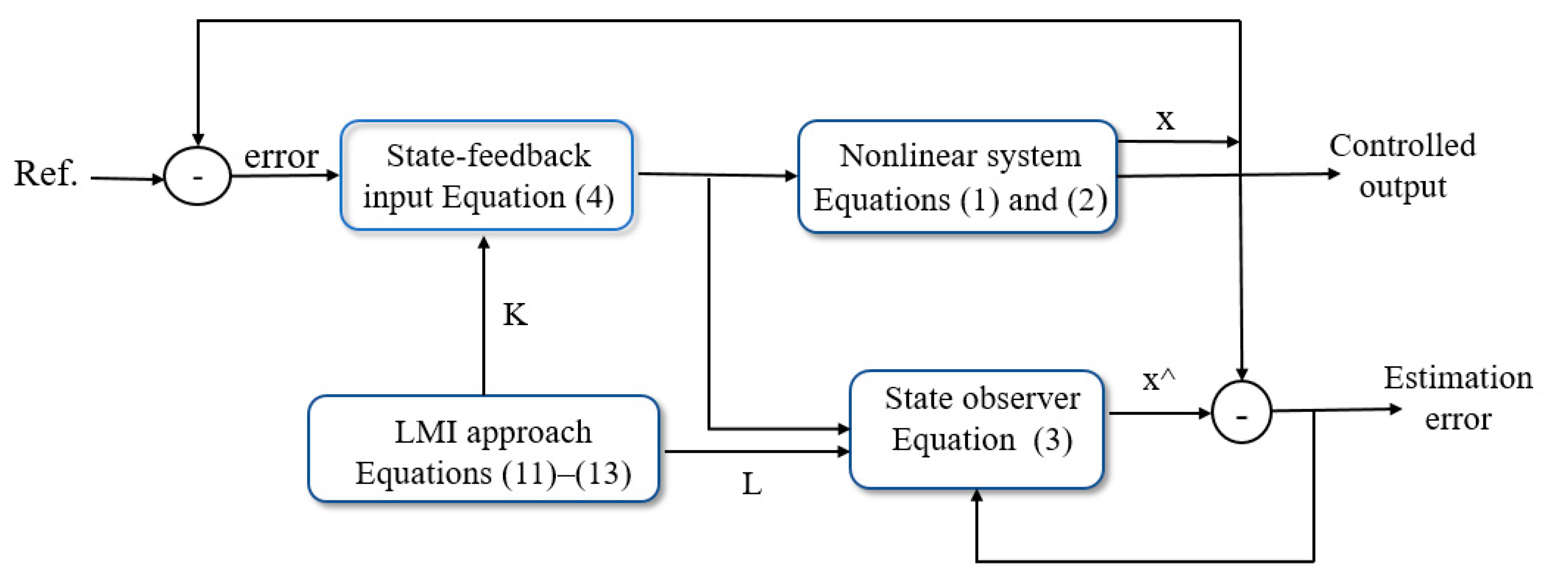
In this work, an observer-based stabilizer for nonlinear systems with external disturbance and an output nonlinear function is designed. Moreover, the LMI method is formulated to obtain the parameters of the planned observer and stabilizer. The asymptotic stabilization of the control system is then achieved and the estimation errors are converged to the origin asymptotically. The block diagram of the proposed strategy is shown in Figure 1. The simulation results of Genesio’s chaotic system in the existence of output nonlinear functions and exterior perturbations validate the efficacy of the designed approach. Power systems are the important applications of this paper theory [36].

This article has five sections as follows: in Section 2, the necessary preliminaries and problem description are presented. In Section 3, the proposed stabilizer and observer are designed, their parameters are calculated by LMIs and the stability of the closed-loop system is proven. In Section 4, the proposed stabilizers are employed to numerical examples and the conclusions are given in Section 5.

2. Problem Description

Consider the following nonlinear state-space system:

$$\dot{x}=Ax+Bu+B_{\omega }\omega \left(t\right)+E_{1}f\left(x\right)$$

(1)

$$y=Cx+Du+E_{2}g\left(x\right)$$

(2)

where $x$ represent the variable state vector of the system, $u\left(t\right)$ shows the controller input, $f\left(x\right)$ is the time-varying nonlinear perturbation, g(x) denotes the nonlinear perturbation that is in the output, $y\left(t\right)$ is the system output and $\omega \left(t\right)$ is the disturbance. A, B, C, D, $E_1$ and $E_2$ are constant matrices. B_ω is the coefficient matrix of the disturbance and B is an invertible matrix.

An observer is defined as:

$$\dot{\widehat{x}}=A\widehat{x}+Bu+L\left(y-\widehat{y}\right)+f\left(\widehat{x}\right)$$

(3)

where the estimated states vector is denoted by $\widehat{x}$ and L is the gain of the state observer. The system (1–2) controller is the state feedback and is designed as:

$$u=K\widehat{x}-B^{-1}{E}_{1}f\left(\widehat{x}\right)-B^{-1}{E}_2\left(g\left(x\right)-g\left(\widehat{x}\right)\right).$$

(4)

The error of estimation is defined as $e=x-\widehat{x}$, where using (2–3), the following Equation is attained:

$$\dot{e}=\left(A-LC\right)e+B_{\omega }\omega +E_1\left(f\left(x\right)-f\left(\widehat{x}\right)\right)-L{E}_2\left(g\left(x\right)-g\left(\widehat{x}\right)\right).$$

(5)

Substituting Equation (4) into Equation (1), we have:

$$\dot{x}=\left(A+BK\right)x-BKe+E_1\left(f\left(x\right)-f\left(\widehat{x}\right)\right)-E_2\left(g\left(x\right)-g\left(\widehat{x}\right)\right)+B_{\omega }\omega .$$

(6)

From Equations (5) and (6), the closed-loop system is represented as:

$$\begin{array}{c}\left[\begin{array}{c}\dot{x}\\ \dot{e}\end{array}\right]=\left[\begin{array}{cc}A+BK& -BK\\ 0& A-LC\end{array}\right]\left[\begin{array}{c}x\\ e\end{array}\right]+\left[\begin{array}{cc}{E}_1& -E_1\\ E_1& -E_1\end{array}\right]\left[\begin{array}{c}f\left(x\right)\\ f\left(\widehat{x}\right)\end{array}\right]+\left[\begin{array}{cc}{E}_2& -E_2\\ L{E}_2& -L{E}_2\end{array}\right]\left[\begin{array}{c}g\left(x\right)\\ g\left(\widehat{x}\right)\end{array}\right]\\ +\left[\begin{array}{cc}{B}_{\omega }& 0\\ 0& B_{\omega }\end{array}\right]\left[\begin{array}{c}\omega \\ \omega \end{array}\right]\end{array}$$

(7)

Assumption 1.

The functions$f\left(x\right)$and$g\left(x\right)$are called Lipschitz continuous if the constants${\mathsf{\Omega }}_1,{\mathsf{\Omega }}_2>0$exist and satisfy:

$$\left|\left|f\left(x\right)-f\left(\widehat{x}\right)\left|\left|\le {\mathsf{\Omega }}_1\right|\right|x-\widehat{x}\right|\right|$$

(8)

$$\left|\left|g\left(x\right)-g\left(\widehat{x}\right)\left|\left|\le {\mathsf{\Omega }}_2\right|\right|x-\widehat{x}\right|\right|$$

(9)

where${\mathsf{\Omega }}_1$and${\mathsf{\Omega }}_2$denote the Lipschitz constants.

An optimization-based algorithm is proposed in [37] to calculate the Lipschitz constant associated with any given nonlinear function on its predefined domain.

The Schur complement lemma [38] is employed to transform the convex nonlinear inequality to an LMI. If M is an $n\times n$ Hermitian matrix $M=\left[\begin{array}{cc}{M}_{11}& M_{12}\\ {M_{12}}^T& M_{22}\end{array}\right]$, in which $M_{11}={M_{11}}^T$ and $M_{22}={M_{22}}^T$, if $M_{22}$ is invertible, then $M<0$ is equivalent to $M_{11}-M_{12}{M_{22}}^{-1}{M}_{21}<0$ and $M_{22}<0$.

3. Main Results

3.1. Systems with a Nonlinear Function and Disturbance

The first problem is that nonlinear systems depend on the system states, disturbance and linear outputs. The state-space form of the control system is as the following equation:

$$\{\begin{array}{c}\dot{x}=Ax+Bu+B_{\omega }\omega +f\left(x\right)\\ y=Cx+Du\end{array}$$

(10)

where Equation (10) is equal to Equations (1) and (2) in which $E_2$ is zero and $E_1$ is an identity matrix. Therefore, in order to verify the stability of the closed-loop system with the controller signal (4) and the state observer (3), the following theorem should be considered.

Theorem 1.

The system model in Equation (10) and the observer (3) guarantee Assumption 1. If there exists symmetric matrices $Q_1$, Q₂$\in R^{n\times n}$whereQ₁, Q₂ > 0 and Q₁ = Q₁^T, Q₂ = Q₂^T such that guarantees the following LMIs:

$$\left[\begin{array}{cc}\frac{1}{\lambda }{Q}_1& 0\\ \ast & Q_2\end{array}\right]>0$$

(11)

$$\left[\begin{array}{ccccc}{A}^T{Q}_2-C^T{P_2}^T+Q_{2}A-P_{2}C& Q_2{B}_{\omega }& Q_2& {{\mathsf{\Omega }}_1}^T& I\\ \ast & -\gamma & 0& 0& 0\\ \ast & \ast & -I& 0& 0\\ \ast & \ast & \ast & -I& 0\\ \ast & \ast & \ast & \ast & -\gamma \end{array}\right]<0$$

$$\left[\begin{array}{cc}\frac{1}{\lambda }\left(AM+B{P}_1+M{A}^T+{P_1}^T{B}^T\right)& M\\ \ast & -\gamma I\end{array}\right]<0$$

(12)

where using K = P₁Q₁, L = Q₂⁻¹P₂ and M = Q₁⁻¹, the signal of control (4) guarantees that the output of the system satisfies $sup\frac{|\left|y\right|{|}_{L2}}{|\left|\omega \right|{|}_{L2}}<\gamma$ and the states of the system are asymptotically stable.

Proof. 

Consider the Lyapunov candidate functional for system (7) as follows:

$$V\left(X\right)=X^{T}QX$$

(13)

where $X=\left[\begin{array}{c}x\\ e\end{array}\right]$, $Q=\left[\begin{array}{cc}\frac{1}{\lambda }{Q}_1& 0\\ 0& Q_2\end{array}\right]$ denotes a positive-definite matrix and $\lambda$ represents a positive constant. The cost function is considered as:

$$J=\frac{\left(\dot{V}+x^T{C^{\prime }}^T{C}^{\prime }x-{\gamma }^2{\omega }^T\omega \right)}{\gamma }<0$$

(14)

where $C^{\prime }=\left[I\hspace{1em}0\right]$. By taking the time-derivative of V(X) and replacing it into Equation (14), the following inequality is obtained:

$$\begin{array}{cc}J=\hfill & x^T\left(\left(A^T+K^T{B}^T\right)\frac{1}{\lambda }{Q}_1+\frac{1}{\lambda }{Q}_1\left(A+BK\right)+\frac{1}{\gamma }I\right)x\hfill \\ & +x^T\left(-\frac{1}{\lambda }{Q}_{1}BK-\frac{1}{\gamma }I\right)e-e^T\left(\frac{1}{\lambda }{Q}_1{K}^T{B}^T+\frac{1}{\gamma }I\right)x\hfill \\ & +e^T\left(\left(A^T-C^T{L}^T\right)Q_2+Q_2\left(A-LC\right)+\frac{1}{\gamma }I\right)e\hfill \\ \hfill +& \frac{1}{\lambda }{x}^T{Q}_1\left(f\left(x\right)-f\left(\widehat{x}\right)\right)+e^T{Q}_2\left(f\left(x\right)-f\left(\widehat{x}\right)\right)\hfill \\ & +\frac{1}{\lambda }\left(f^T\left(x\right)-f^T\left(\widehat{x}\right)\right)Q_{1}x+\left(f^T\left(x\right)-f^T\left(\widehat{x}\right)\right)Q_{2}e-\gamma {\omega }^T\omega \hfill \\ & +\frac{1}{\lambda }{\omega }^T{B_{\omega }}^T{Q}_{1}x+{\omega }^T{B_{\omega }}^T{Q}_{2}e+\frac{1}{\lambda }{x}^T{Q}_1{B}_{\omega }\omega +e^T{Q}_2{B}_{\omega }\omega <0\hfill \end{array}$$

(15)

Equation (8) can be rewritten as below:

$${(f\left(x\right)-f\left(\widehat{x}\right))}^{T}I\left(f\left(x\right)-f\left(\widehat{x}\right)\right)\le e^T{{\mathsf{\Omega }}_1}^T{\mathsf{\Omega }}_{1}e.$$

(16)

From (15) and (16), the result can be written in a quadratic inequality form as:

$$Z^T\psi Z<0$$

(17)

where:

$$Z={\left[xe\omega \left(f\left(x\right)-f\left(\widehat{x}\right)\right)\right]}^T$$

(18)

$$\psi =\left[\begin{array}{cccc}{\sum }_1& {\sum }_2& \frac{1}{\lambda }{Q}_1{B}_{\omega }& \frac{1}{\lambda }{Q}_1\\ \ast & {\sum }_3& Q_2{B}_{\omega }& Q_2\\ \ast & \ast & -\gamma & 0\\ \ast & \ast & \ast & -I\end{array}\right]<0$$

(19)

with:

$${{\displaystyle \sum }}_1=\frac{1}{\lambda }{Q}_1\left(A+BK\right)+\left(A^T+K^T{B}^T\right)\frac{1}{\lambda }{Q}_1+\frac{1}{\gamma }I$$

(20)

$${{\displaystyle \sum }}_2=-\frac{1}{\lambda }{Q}_{1}BK-\frac{1}{\gamma }I$$

(21)

$${{\displaystyle \sum }}_3=\left(A^T-C^T{L}^T\right)Q_2+Q_2\left(A-LC\right)+\frac{1}{\gamma }I+{{\mathsf{\Omega }}_1}^T{\mathsf{\Omega }}_1.$$

(22)

By pre-and post-multiplying (19) to $\mathrm{diag}\left({Q_1}^{-1},I,I,I\right)$, one can obtain:

$$\left[\begin{array}{cccc}{\prod }_1& {\prod }_2& \frac{1}{\lambda }{B}_{\omega }& \frac{1}{\lambda }\\ \ast & {\prod }_3& Q_2{B}_{\omega }& Q_2\\ \ast & \ast & -\gamma & 0\\ \ast & \ast & \ast & -I\end{array}\right]<0$$

(23)

where:

$${\prod }_1=\frac{1}{\lambda }\left(A+BK\right){Q_1}^{-1}+{Q_1}^{-1}\left(A^T+K^T{B}^T\right)\frac{1}{\lambda }+{Q_1}^{-1}\frac{1}{\gamma }{Q_1}^{-1}$$

(24)

$${\prod }_2=-\frac{1}{\lambda }BK-\frac{1}{\gamma }{Q_1}^{-1}I$$

(25)

$${\prod }_3=\left(A^T-C^T{L}^T\right)Q_2+Q_2\left(A-LC\right)+\frac{1}{\gamma }I+{{\mathsf{\Omega }}_1}^T{\mathsf{\Omega }}_1.$$

(26)

Now, using the Schur complement lemma and considering $L={Q_2}^{-1}{P}_2$, $M={Q_1}^{-1}$, $K=P_1{Q}_1$ and $\lambda \to 0$, the LMIs in Theorem 1 are established and the control law and observer gains K and L are obtained. □

3.2. Systems with Nonlinear Outputs

In this part, the systems are considered with a nonlinear output and without disturbances as follows:

$$\{\begin{array}{c}\dot{x}=Ax+Bu+E_{1}f\left(x\right)\\ y=Cx+Du+E_{2}g\left(x\right)\end{array}.$$

(27)

By applying the control input (4) and state observer (3), the closed-loop system stability is proven.

Theorem 2.

If the system (1) and observer (3) satisfy Assumption 1 and there exists two$n\times n$symmetric matrices Q₁ and Q₂ where Q₁, Q₂ > 0 and Q₁ = Q₁^T, Q₂ = Q₂^T, it will fulfil the following LMIs:

$$\left[\begin{array}{cc}\frac{1}{\lambda }{Q}_1& 0\\ \ast & Q_2\end{array}\right]>0$$

(28)

$$\left[\begin{array}{ccccc}{A}^T{Q}_2-C^T{P_2}^T+Q_{2}A-P_{2}C& Q_2{E}_2& -P_2{E}_2& {{\mathsf{\Omega }}_1}^{T}I& {{\mathsf{\Omega }}_2}^{T}I\\ \ast & -I& 0& 0& 0\\ \ast & \ast & -I& 0& 0\\ \ast & \ast & \ast & -I& 0\\ \ast & \ast & \ast & \ast & -I\end{array}\right]<0$$

(29)

$$\frac{1}{\lambda }\left(AM+B{P}_1+M{A}^T+{P_1}^T{B}^T\right)<0$$

(30)

where using K = P₁Q₁, L = Q₂⁻¹P₂ and M = Q₁⁻¹, the states of the system are asymptotically stable.

Proof. 

Consider the Lyapunov candidate functional for system (7) as follows:

$$V\left(X\right)=X^{T}QX$$

(31)

where $X=\left[\begin{array}{c}x\\ e\end{array}\right]$, $Q=\left[\begin{array}{cc}\frac{1}{\lambda }{Q}_1& 0\\ 0& Q_2\end{array}\right]$ denotes a positive-definite matrix and $\lambda$ means a positive constant. To prove the stability of the system, the term $\dot{V}\left(X\right)$ must be negative-definite. Therefore, by the time-derivative of Equation (31), the following inequality is obtained:

$${\left[\begin{array}{c}x\\ e\\ f(x)-f(\widehat{x})\\ g(x)-g(\widehat{x})\end{array}\right]}^T\mathsf{\Upsilon }\left[\begin{array}{c}x\\ e\\ f(x)-f(\widehat{x})\\ g(x)-g(\widehat{x})\end{array}\right]<0$$

(32)

where:

$$\mathsf{\Upsilon }=\left[\begin{array}{cccc}{\sum }_1& {\sum }_2& \frac{1}{\lambda }{Q}_1{E}_1& -\frac{1}{\lambda }{Q}_1{E}_2\\ \ast & {\sum }_3& Q_2{E}_2& -Q_{2}L{E}_2\\ \ast & \ast & 0& 0\\ \ast & \ast & \ast & 0\end{array}\right]$$

(33)

with ${{\displaystyle \sum }}_1=\frac{1}{\lambda }{Q}_1\left(A+BK\right)+\left(A^T+K^T{B}^T\right)\frac{1}{\lambda }{Q}_1$, ${{\displaystyle \sum }}_2=-\frac{1}{\lambda }{Q}_{1}BK$ and ${{\displaystyle \sum }}_3=\left(A^T-C^T{L}^T\right)Q_2+Q_2\left(A-LC\right).$ Assumption 1 can be rewritten as:

$${\left[\begin{array}{c}x\\ e\\ f(x)-f(\widehat{x})\\ g(x)-g(\widehat{x})\end{array}\right]}^T\prod \left[\begin{array}{c}x\\ e\\ f(x)-f(\widehat{x})\\ g(x)-g(\widehat{x})\end{array}\right]>0$$

(34)

where:

$$\prod =\left[\begin{array}{cccc}0& 0& 0& 0\\ \ast & {\mathsf{\Omega }}_1^T{\mathsf{\Omega }}_1+{\mathsf{\Omega }}_2^T{\mathsf{\Omega }}_2& 0& 0\\ \ast & \ast & -I& 0\\ \ast & \ast & \ast & -I\end{array}\right].$$

(35)

Equation (34) is added to (32), thereby satisfying the inequality (32), and the following matrix should be negative:

$$\left[\begin{array}{cccc}{\sum }_1& {\sum }_2& \frac{1}{\lambda }{Q}_1{E}_1& -\frac{1}{\lambda }{Q}_1{E}_2\\ \ast & {\sum }_3+{\mathsf{\Omega }}_1^T{\mathsf{\Omega }}_1+{\mathsf{\Omega }}_2^T{\mathsf{\Omega }}_2& Q_2{E}_2& -Q_{2}L{E}_2\\ \ast & \ast & -I& 0\\ \ast & \ast & \ast & -I\end{array}\right]<0.$$

(36)

By pre-and post-multiplying the inequality (36) to $\mathrm{diag}\left({Q_1}^{-1},I,I,I\right)$, one can obtain:

$$\left[\begin{array}{cccc}{\prod }_1& {\prod }_2& \frac{1}{\lambda }{E}_1& -\frac{1}{\lambda }{E}_2\\ \ast & {\prod }_3& Q_2{E}_2& -Q_{2}L{E}_2\\ \ast & \ast & -I& 0\\ \ast & \ast & \ast & -I\end{array}\right]<0$$

(37)

where ${\prod }_1=\frac{1}{\lambda }\left(A+BK\right){Q_1}^{-1}+{Q_1}^{-1}\left(A^T+K^T{B}^T\right)\frac{1}{\lambda }$,${\prod }_2=-\frac{1}{\lambda }BK$, ${\prod }_3=\left(A^T-C^T{L}^T\right)Q_2+Q_2\left(A-LC\right)+{{\mathsf{\Omega }}_1}^T{\mathsf{\Omega }}_1+{{\mathsf{\Omega }}_2}^T{\mathsf{\Omega }}_2$; then using the Schur complement lemma, by taking $M={Q_1}^{-1}$, $L={Q_2}^{-1}{P}_2$,$K=P_1{Q}_1$ and $\lambda \to 0$, this theorem is proven. As a result, similar to [39], the proposed theorems have sufficient conditions of the global solution’s existence and stabilization at infinity to the equilibrium point. □

4. Simulation Results

In this part, a Genesio chaotic system is utilized to demonstrate the validation of the suggested method, which is defined as [40]:

$$\{\begin{array}{c}{\dot{x}}_1=x_2\\ {\dot{x}}_2=x_3\\ {\dot{x}}_3=-c{x}_1-b{x}_2-a{x}_3+x_1^2\end{array}$$

(38)

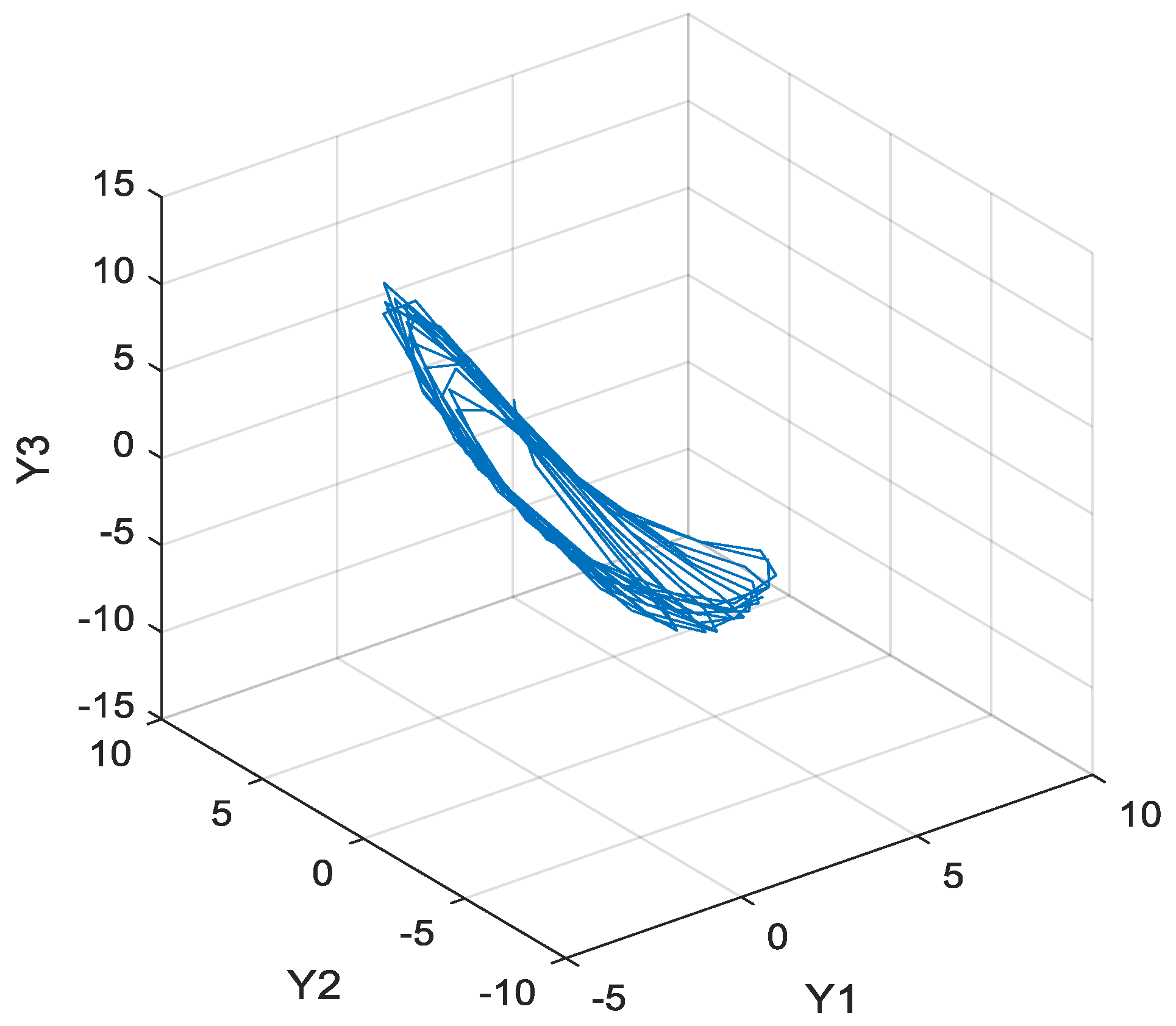
The trajectory of the states of the chaotic system is shown in Figure 2. The Genesio chaotic system has a nonlinear behavior that is sensitive to changes in the system parameters and the initial conditions. The system signals have strong harmonics. With motion in the phase space, it has an irregular performance.

4.1. A Genesio System with a Nonlinear Function and Disturbance

The model of a Genesio system with a Lipschitz nonlinear perturbation and disturbance is as follows:

$$\{\begin{array}{c}{\dot{x}}_1=x_2+0.1\cos (2t)+u_1\\ {\dot{x}}_2=x_3+0.15\cos (3t)+u_2\\ {\dot{x}}_3=-6x_1-2.92x_2-1.2x_3+0.2\cos (4t)+x_1^2+u_3\end{array}.$$

(39)

To use the proposed control method, Equation (39) is expressed as:

$$\begin{array}{c}\left[\begin{array}{c}{\dot{x}}_1\left(t\right)\\ {\dot{x}}_2\left(t\right)\\ {\dot{x}}_3\left(t\right)\end{array}\right]=\left[\begin{array}{ccc}0& 1& 0\\ 0& 0& 1\\ -6& -2.92& -1.2\end{array}\right]\left[\begin{array}{c}{x}_1\left(t\right)\\ x_2\left(t\right)\\ x_3\left(t\right)\end{array}\right]\\ +\left[\begin{array}{ccc}1& 0& 0\\ 0& 1& 0\\ 0& 0& 1\end{array}\right]u\left(t\right)+\left[\begin{array}{c}0\\ 0\\ {x_1}^2\left(t\right)\end{array}\right]+d\\ y=\left[\begin{array}{ccc}1& 0& 0\\ 0& 1& 0\\ 0& 0& 1\end{array}\right]\left[\begin{array}{c}{x}_1\left(t\right)\\ x_2\left(t\right)\\ x_3\left(t\right)\end{array}\right].\end{array}$$

(40)

According to the dynamics of Genesio’s system (40) and Equation (10), the nonlinear part of the dynamical system is:

$$f\left(x\right)=\left[\begin{array}{c}0\\ 0\\ {x_1}^2\left(t\right)\end{array}\right]$$

where the Lipschitz constant can be obtained from:

$$\mathsf{\Omega }=\max \left\{\frac{\partial f}{\partial x_1},\frac{\partial f}{\partial x_2},\frac{\partial f}{\partial x_3}\right\}.$$

(41)

The disturbance and parametric nonlinear function are considered as $d={\left[0.1\cos (2t)\hspace{1em}0.15\cos (3t)\hspace{1em}0.2\cos (4t)\right]}^T$, $f={\left[0\hspace{1em}0\hspace{1em}{x_1}^2\right]}^T$. For the simulation, consider the initial values and the Lipschitz constant as $x\left(0\right)=\left[4\hspace{1em}3\hspace{1em}-4\right]$, $\widehat{x}\left(0\right)=\left[0\hspace{1em}0\hspace{1em}1\right]$ and Ω = 2. The achieved parameters $L,K$ and $\gamma$ by MATLAB YALMIP toolbox are as follows:

$$K=\left[\begin{array}{ccc}-55.5923& -0.5& 3\\ -0.5& -55.5923& 0.96\\ 3& 0.96& -54.3923\end{array}\right]L=\left[\begin{array}{ccc}70.7050& 0.5& -1.9104\\ 0.6347& 97.8047& -0.6801\\ -3& -0.8414& 123.9110\end{array}\right] , \gamma =0.0663.$$

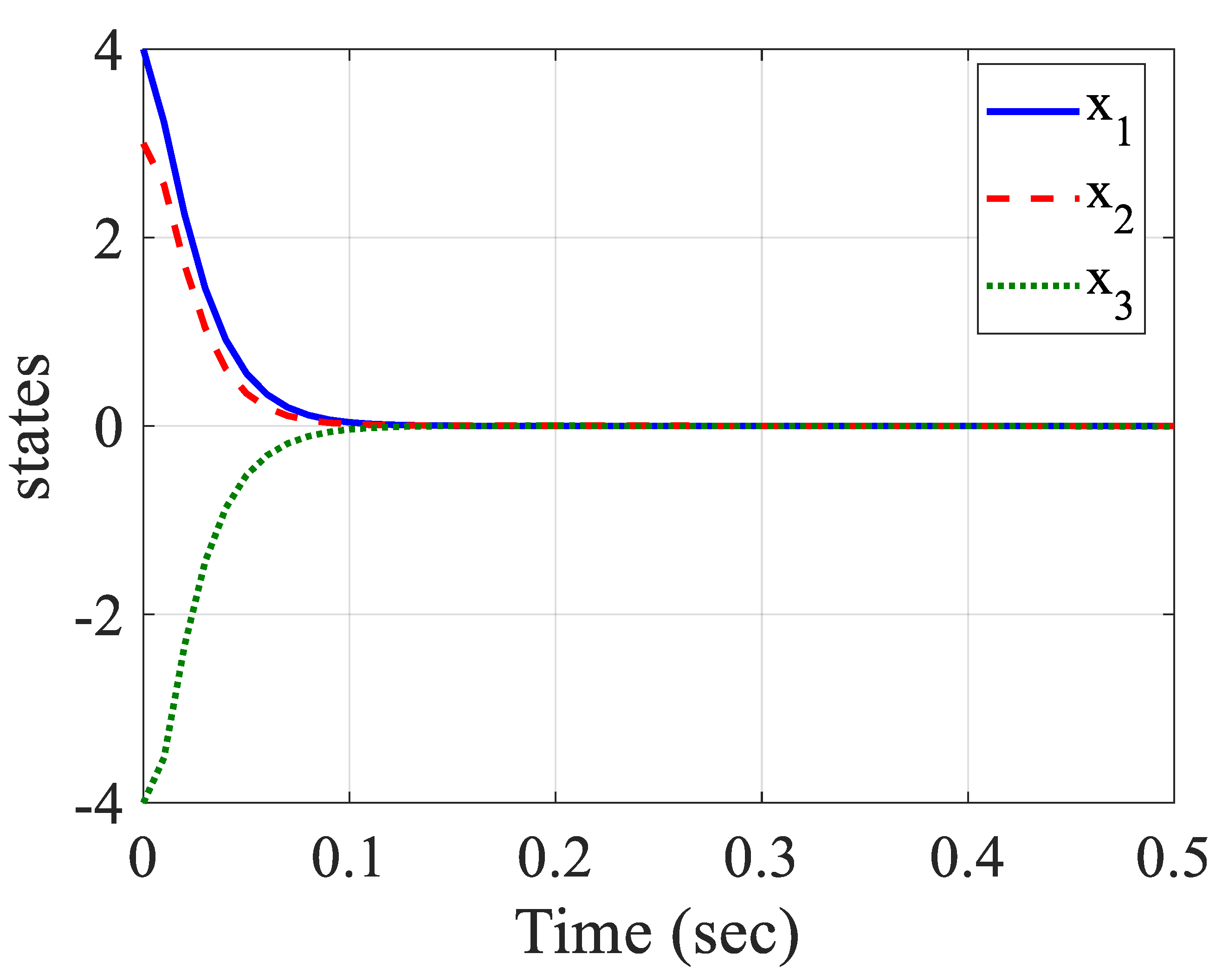
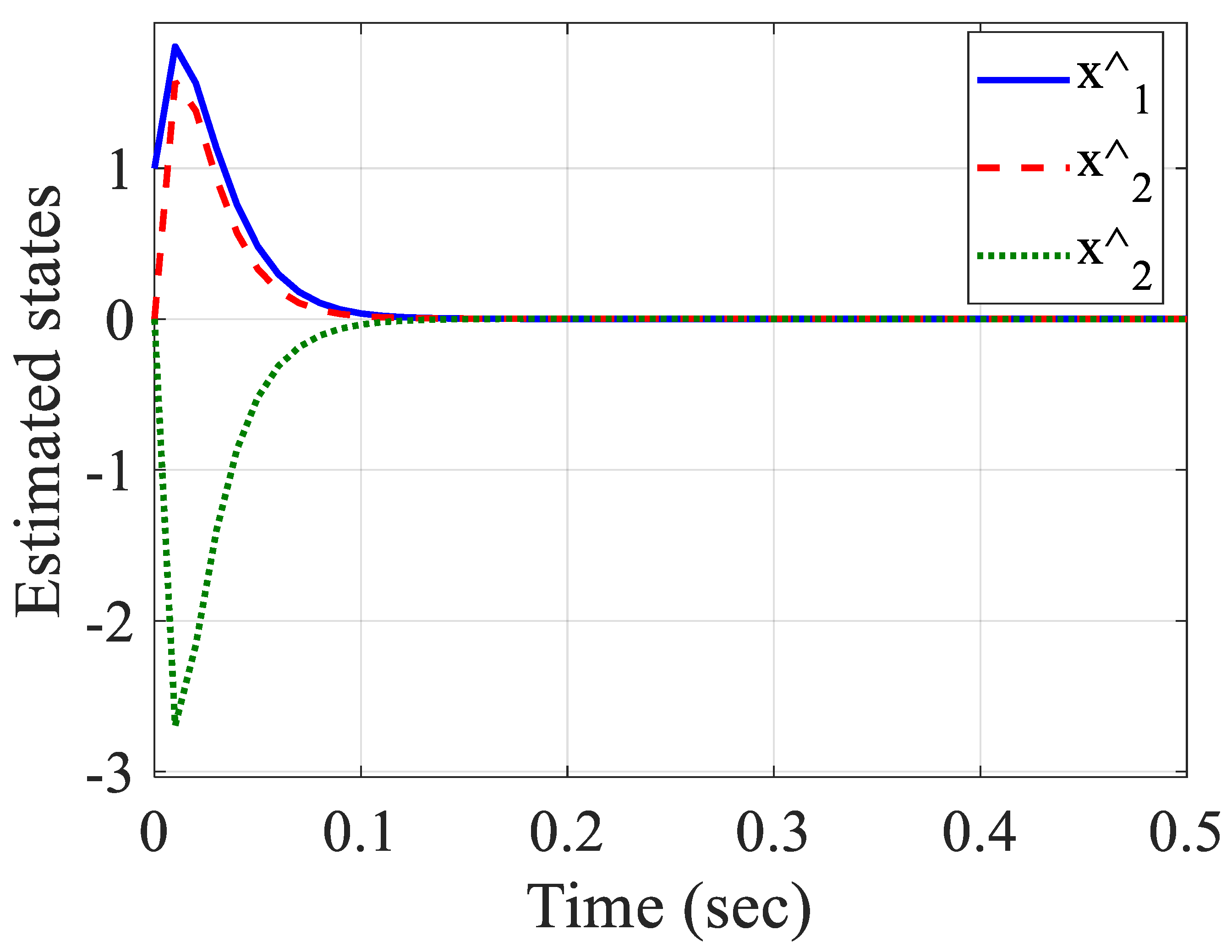
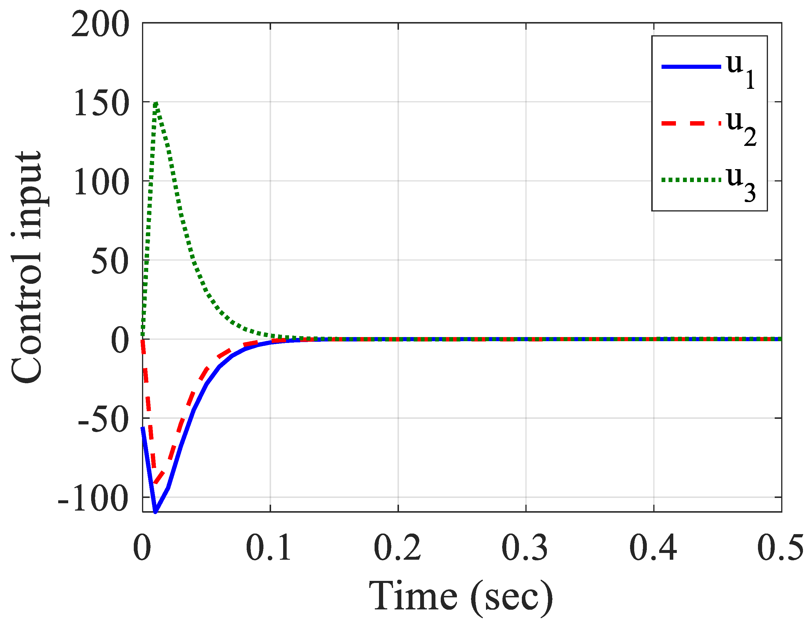
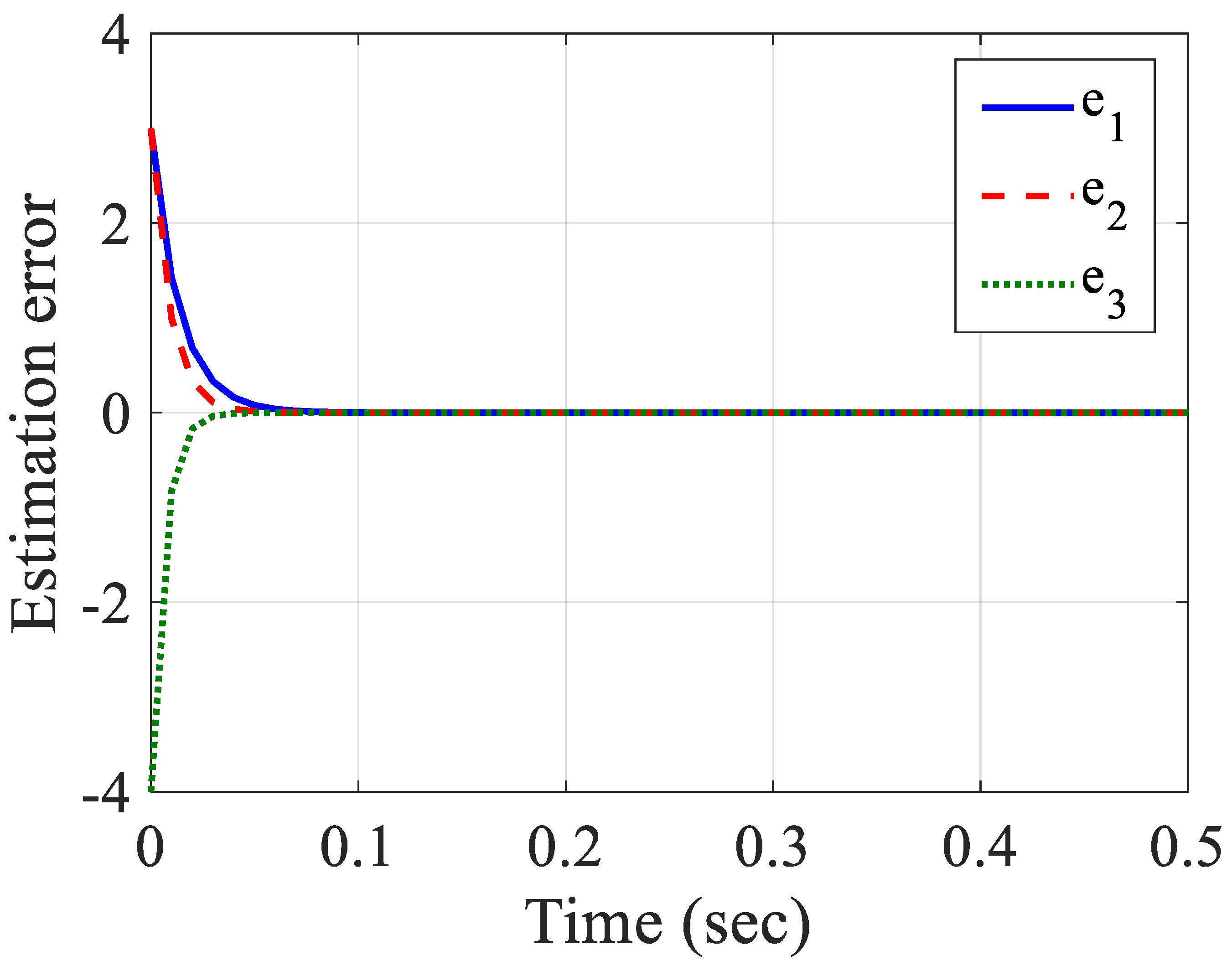
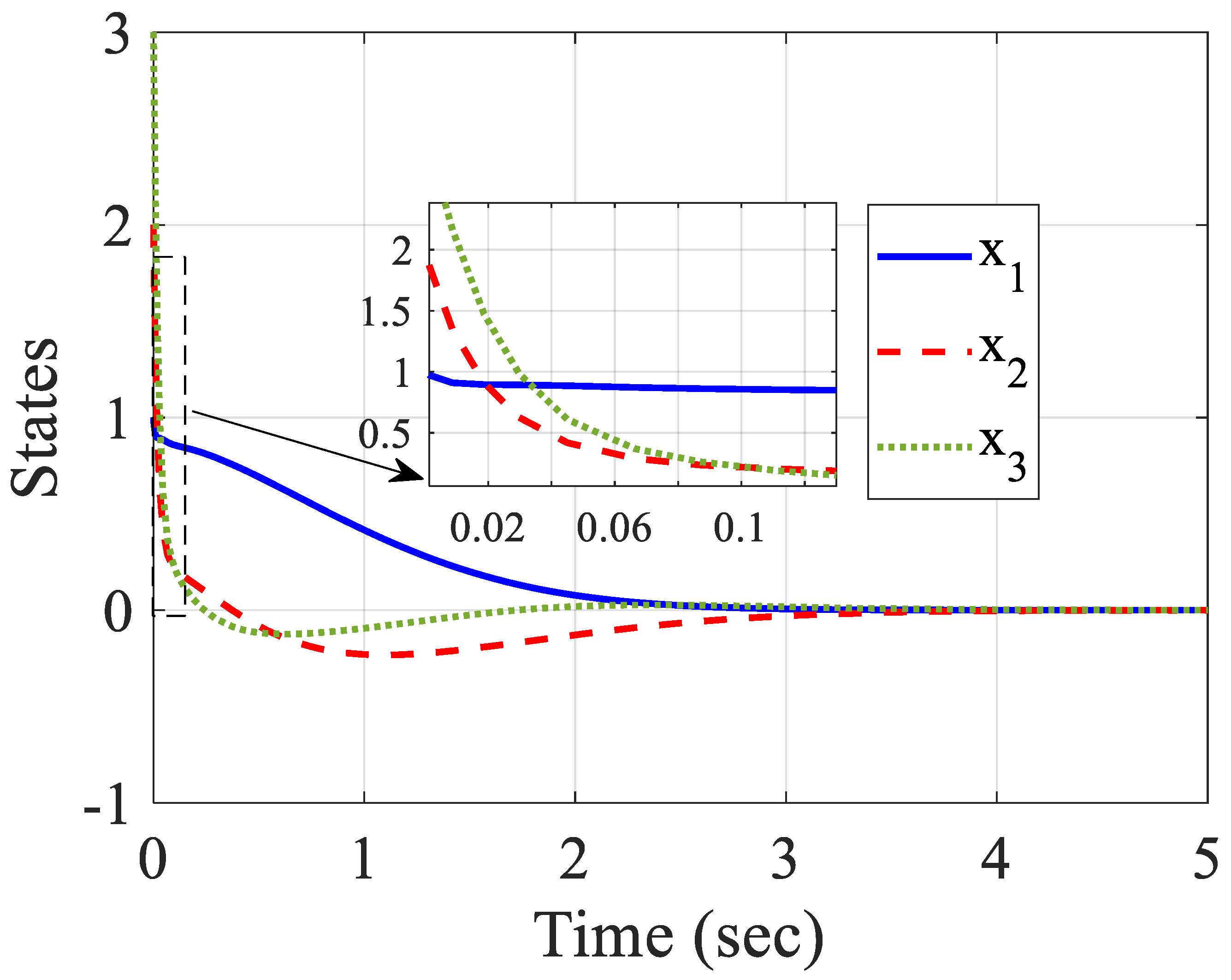
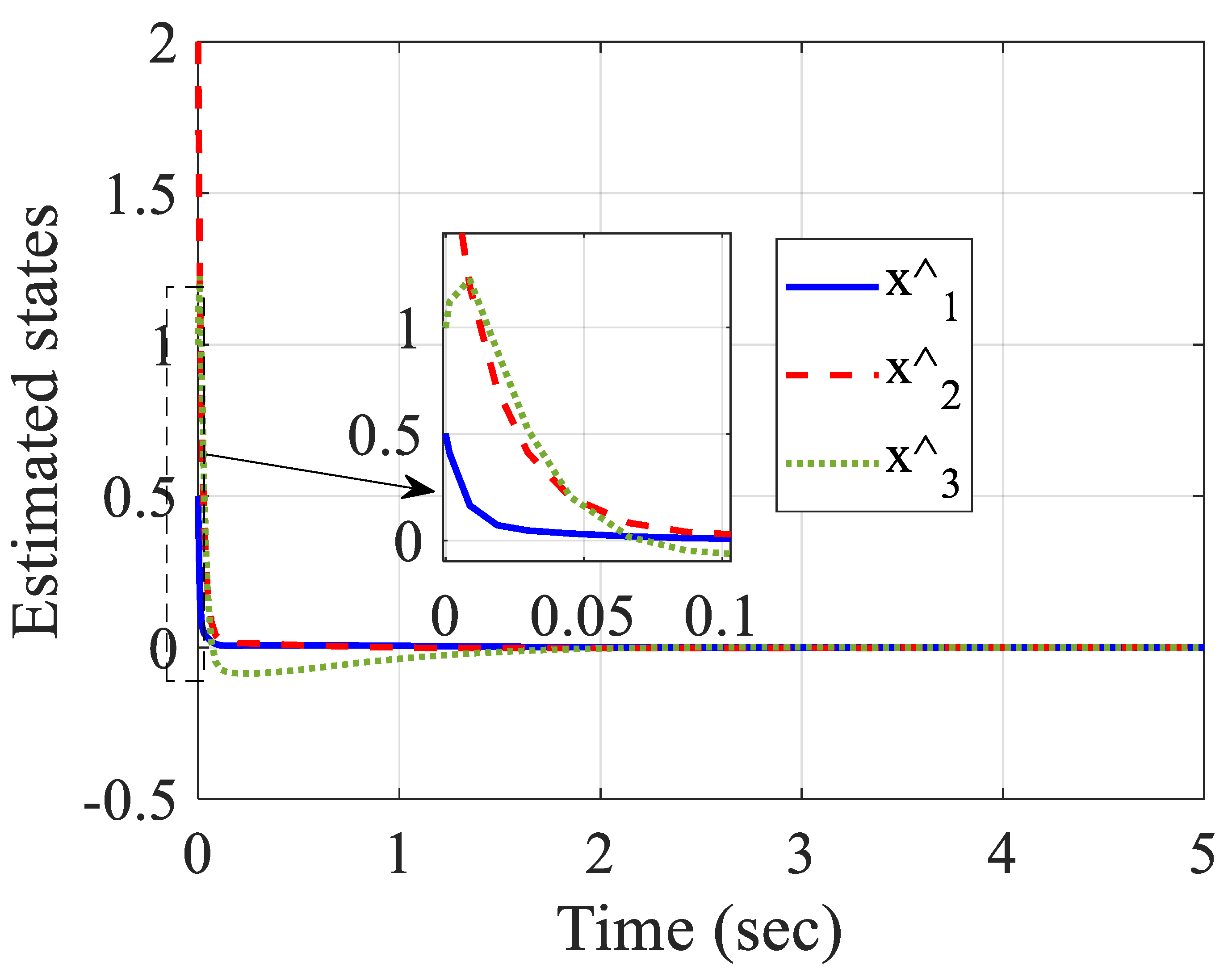
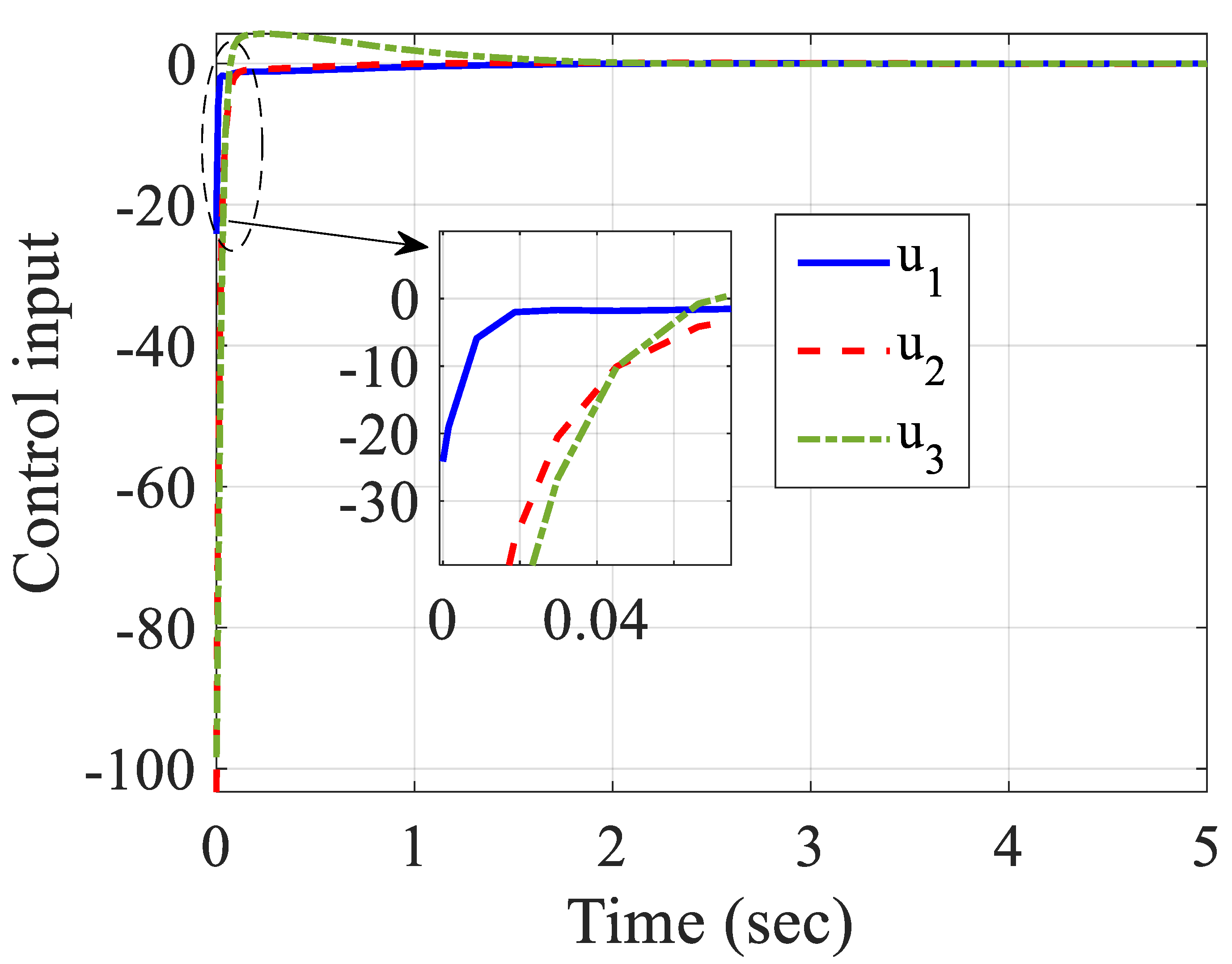
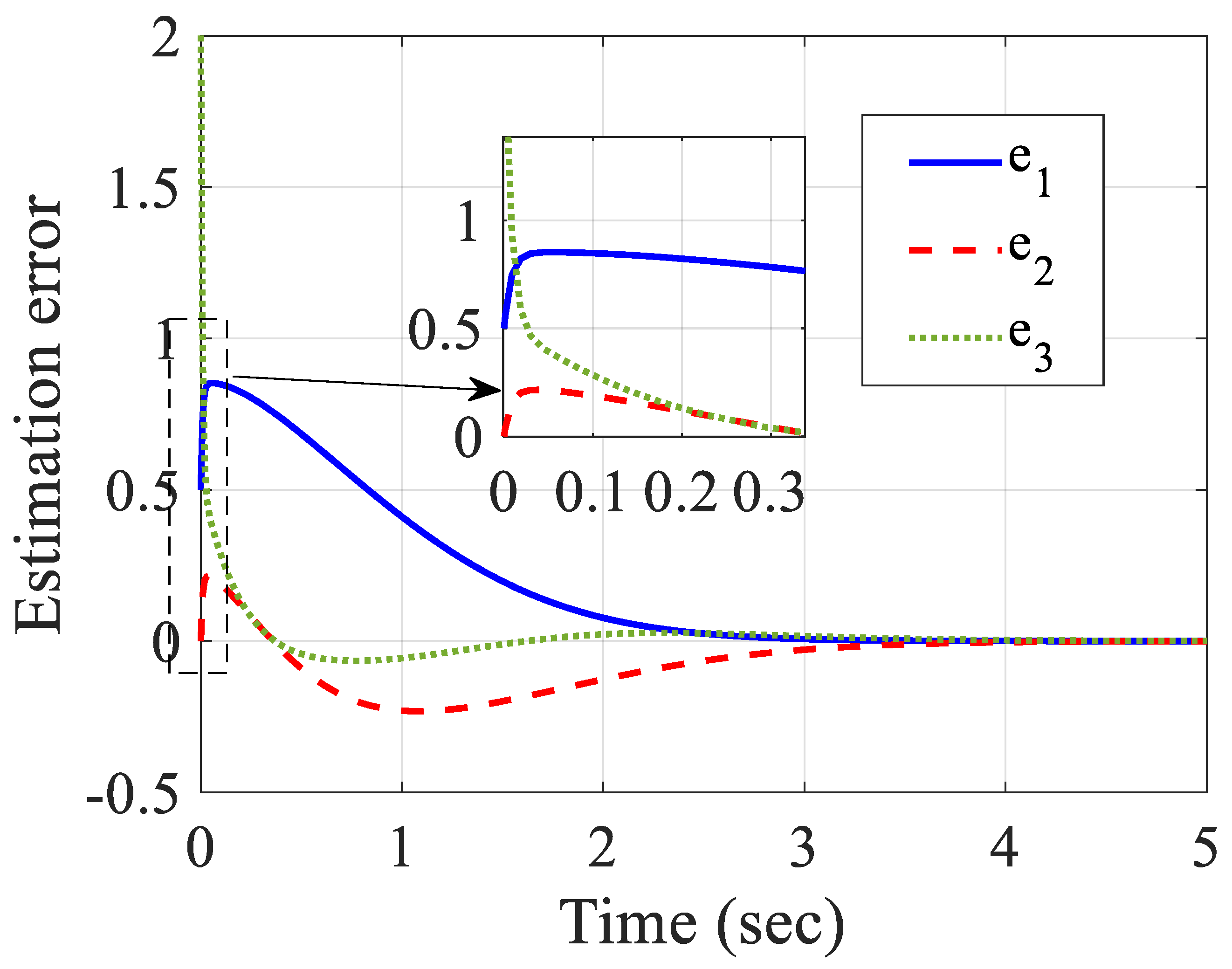
Figure 3, Figure 4, Figure 5 and Figure 6 demonstrate the system states, estimated states, signal of the control input and state estimation errors. Figure 3 depicts the convergence of states to zero during 0.1 s and with no chattering. Figure 4 displays that the states were properly estimated and the convergence of them, which is clear that if the states were inaccessible, the suggested method could estimate the states well. Figure 5 demonstrates the control inputs that show the control signals with appropriate amplitudes. Figure 6 illustrates that the error of estimation converged to zero; it shows the good performance of the Luenberger observer in which its gain was obtained from the LMI and the system was stabilized. As is clear from the figures, the asymptotic stabilization of system in 0.1 s was completed and the observer accuracy was significant.

4.2. A Genesio System with an Output Nonlinear Function

The considered approach in the second theorem was applied on a Genesio system with an output nonlinear function as explained with the following model:

$$\begin{array}{c}\left[\begin{array}{c}{\dot{x}}_1\left(t\right)\\ {\dot{x}}_2\left(t\right)\\ {\dot{x}}_3\left(t\right)\end{array}\right]=\left[\begin{array}{ccc}0& 1& 0\\ 0& 0& 1\\ -6& -2.92& -1.2\end{array}\right]\left[\begin{array}{c}{x}_1\left(t\right)\\ x_2\left(t\right)\\ x_3\left(t\right)\end{array}\right]\\ +\left[\begin{array}{ccc}1& 0& 0\\ 0& 1& 0\\ 0& 0& 1\end{array}\right]u\left(t\right)+\left[\begin{array}{c}0\\ 0\\ {x_1}^2\left(t\right)\end{array}\right]\\ y=\left[\begin{array}{ccc}1& 0& 0\\ 0& 1& 0\\ 0& 0& 1\end{array}\right]\left[\begin{array}{c}{x}_1\left(t\right)\\ x_2\left(t\right)\\ x_3\left(t\right)\end{array}\right]+\left[\begin{array}{ccc}1& 0& 0\\ 0& 1& 0\\ 0& 0& 1\end{array}\right]u\left(t\right)+\left[\begin{array}{c}{x_1}^3\left(t\right)\\ 0\\ 0\end{array}\right]\end{array}$$

(42)

For simulation, consider the initial values as $x\left(0\right)=\left[1\hspace{1em}2\hspace{1em}3\right]$, $\widehat{x}\left(0\right)=\left[0.5\hspace{1em}2\hspace{1em}1\right]$ and from Equation (41), take the Lipschitz constants ${\mathsf{\Omega }}_1=2, {\mathsf{\Omega }}_2=3$. The achieved parameters of $K$ and $L$ via MATLAB YALMIP toolbox are obtained as:

$$K=\left[\begin{array}{ccc}-50& -0.5& 3\\ -0.5& -50& 0.96\\ 3& 0.96& -48.8\end{array}\right]; L=\left[\begin{array}{ccc}95.46& 0.0812& -0.8978\\ 0.6433& 1.0979& -0.5139\\ -3.6814& -0.2216& 3.9834\end{array}\right].$$

Similar to before, the system state, estimated states, signal controls and state estimation errors are demonstrated in Figure 7, Figure 8, Figure 9 and Figure 10. Figure 7 shows the convergence of the state variables to zero without any overshoot and it was achieved before 3 s. Figure 8 demonstrates the estimated states converging to the origin. It shows the efficiency of the designed observer-based control method that could estimate the unmeasurable states of the system in a short time and stabilize them. Figure 9 depicts the control inputs that stabilized the closed-loop system before two seconds without overshoot and chattering. The estimation error of the observer is demonstrated in Figure 10. From these simulation results, it could be expressed that the suggested control scheme could be applied on nonlinear systems with irregular behavior.

5. Conclusions

In this manuscript, a new controller of state feedback based on a state observer was proposed for a category of nonlinear systems in the existence of a nonlinear function and disturbance utilizing LMIs and the theory of Lyapunov stability. For the elimination of the effect of the output nonlinear function, the minimization of the effect of disturbance and the obtaining of a stabilized system, various mathematical tools were employed. It was depicted in the simulation results that the state variables of the system were estimated by the state observer and the stability of the closed-loop system was proven. The estimation error signals also converged to the origin. Lastly, MATLAB Simulink and the YALMIP toolbox were utilized to solve the LMI and simulate the numerical examples. The simulation results proved the efficiency of the proposed method.

References

- Elloumi, M.; Ghamgui, M.; Mehdi, D.; Tadeo, F.; Chaabane, M. Stability and stabilization of 2d singular systems: A strict lmi approach. Circuits Syst. Signal Process 2019, 38, 3041–3057. [Google Scholar] [CrossRef]
- Ghaffari, V. A Model Predictive Approach to Dynamic Control Law Design in Discrete-Time Uncertain Systems. Circuits Syst. Signal Process 2020, 39, 4829–4848. [Google Scholar] [CrossRef]
- Kim, W.; Suh, S. Suboptimal Disturbance Observer Design Using All Stabilizing Q Filter for Precise Tracking Control. Mathematics 2020, 8, 1434. [Google Scholar] [CrossRef]
- Pujol-Vazquez, G.; Mobayen, S.; Acho, L. Robust Control Design to the Furuta System under Time Delay Measurement Feedback and Exogenous-Based Perturbation. Mathematics 2020, 8, 2131. [Google Scholar] [CrossRef]
- Lin, C.; Wang, Q.-G.; Lee, T.H. An improvement on multivariable PID controller design via iterative LMI approach. Automatica 2004, 40, 519–525. [Google Scholar] [CrossRef]
- Mobayen, S.; Pujol-Vázquez, G. A robust LMI approach on nonlinear feedback stabilization of continuous state-delay systems with Lipschitzian nonlinearities: Experimental validation. Iran. J. Sci. Technol. Trans. Mech. Eng. 2019, 43, 549–558. [Google Scholar] [CrossRef]
- Gritli, H.; Zemouche, A.; Belghith, S. On LMI conditions to design robust static output feedback controller for continuous-time linear systems subject to norm-bounded uncertainties. Int. J. Syst. Sci. 2021, 52, 12–46. [Google Scholar] [CrossRef]
- Nian, Y.; Zheng, Y. Controlling discrete time TS fuzzy chaotic systems via adaptive adjustment. Phys. Procedia 2012, 24, 1915–1921. [Google Scholar] [CrossRef] [Green Version]
- Ge, M.; Chiu, M.-S.; Wang, Q.-G. Robust PID controller design via LMI approach. J. Process Control 2002, 12, 3–13. [Google Scholar] [CrossRef]
- Yu, X.; Liao, F.; Deng, J. Tracking Controller Design with Preview Action for a Class of Lipschitz Nonlinear Systems and its Applications. Circuits Syst. Signal Process 2019, 39, 2922–2947. [Google Scholar] [CrossRef]
- Hu, J. Dynamic output feedback MPC of polytopic uncertain systems: Efficient LMI conditions. IEEE Trans. Circuits Syst. II Express Briefs 2021. [Google Scholar] [CrossRef]
- Mobayen, S.; Baleanu, D.; Tchier, F. Second-order fast terminal sliding mode control design based on LMI for a class of non-linear uncertain systems and its application to chaotic systems. J. Vib. Control 2017, 23, 2912–2925. [Google Scholar] [CrossRef]
- Ma, Y.; Li, W. Application and research of fractional differential equations in dynamic analysis of supply chain financial chaotic system. Chaos Solitons Fractals 2020, 130, 109417. [Google Scholar] [CrossRef]
- Fečkan, M.; Sathiyaraj, T.; Wang, J. Synchronization of butterfly fractional order chaotic system. Mathematics 2020, 8, 446. [Google Scholar] [CrossRef] [Green Version]
- Lin, C.-H.; Hu, G.-H.; Yan, J.-J. Estimation of Synchronization Errors between Master and Slave Chaotic Systems with Matched/Mismatched Disturbances and Input Uncertainty. Mathematics 2021, 9, 176. [Google Scholar] [CrossRef]
- Rajagopal, K.; Akgul, A.; Moroz, I.M.; Wei, Z.; Jafari, S.; Hussain, I. A simple chaotic system with topologically different attractors. IEEE Access 2019, 7, 89936–89947. [Google Scholar] [CrossRef]
- Nik, H.S.; Golchaman, M. Chaos control of a bounded 4D chaotic system. Neural Comput. Appl. 2014, 25, 683–692. [Google Scholar]
- Vaghefpour, H. Nonlinear Vibration and Tip Tracking of Cantilever Flexoelectric Nanoactuators. Iran. J. Sci. Technol. Trans. Mech. Eng. 2020. [Google Scholar] [CrossRef]
- Li, S.-Y.; Gu, K.-R.; Huang, S.-C. A chaotic system-based signal identification Technology: Fault-diagnosis of industrial bearing system. Measurement 2021, 171, 108832. [Google Scholar] [CrossRef]
- Rehan, M.; Hong, K.-S.; Ge, S.S. Stabilization and tracking control for a class of nonlinear systems. Nonlinear Anal. Real World Appl. 2011, 12, 1786–1796. [Google Scholar] [CrossRef]
- Kheloufi, H.; Zemouche, A.; Bedouhene, F.; Boutayeb, M. On LMI conditions to design observer-based controllers for linear systems with parameter uncertainties. Automatica 2013, 49, 3700–3704. [Google Scholar] [CrossRef]
- Wu, R.; Zhang, W.; Song, F.; Wu, Z.; Guo, W. Observer-based stabilization of one-sided Lipschitz systems with application to flexible link manipulator. Adv. Mech. Eng. 2015, 7. [Google Scholar] [CrossRef]
- Choi, H.H. LMI-based nonlinear fuzzy observer-controller design for uncertain MIMO nonlinear systems. IEEE Trans. Fuzzy Syst. 2007, 15, 956–971. [Google Scholar] [CrossRef]
- Xia, Y.; Jia, Y. Robust sliding-mode control for uncertain time-delay systems: An LMI approach. IEEE Trans. Autom. Control 2003, 48, 1086–1091. [Google Scholar]
- Gouaisbaut, F.; Dambrine, M.; Richard, J.-P. Robust control of delay systems: A sliding mode control design via LMI. Syst. Control Lett. 2002, 46, 219–230. [Google Scholar] [CrossRef] [Green Version]
- Wang, H.; Han, Z.-Z.; Xie, Q.-Y.; Zhang, W. Sliding mode control for chaotic systems based on LMI. Commun. Nonlinear Sci. Numer. Simul. 2009, 14, 1410–1417. [Google Scholar] [CrossRef]
- Park, J.H. Controlling chaotic systems via nonlinear feedback control. Chaos Solitons Fractals 2005, 23, 1049–1054. [Google Scholar] [CrossRef]
- Park, J.H.; Kwon, O.; Lee, S.-M. LMI optimization approach to stabilization of Genesio–Tesi chaotic system via dynamic controller. Appl. Math. Comput. 2008, 196, 200–206. [Google Scholar] [CrossRef]
- Kuntanapreeda, S. Chaos synchronization of unified chaotic systems via LMI. Phys. Lett. A 2009, 373, 2837–2840. [Google Scholar] [CrossRef]
- Chen, F.; Zhang, W. LMI criteria for robust chaos synchronization of a class of chaotic systems. Nonlinear Anal. Theory Methods Appl. 2007, 67, 3384–3393. [Google Scholar] [CrossRef]
- Wang, Y.-W.; Guan, Z.-H.; Wang, H.O. LMI-based fuzzy stability and synchronization of Chen’s system. Phys. Lett. A 2003, 320, 154–159. [Google Scholar] [CrossRef]
- Park, J.H.; Kwon, O. LMI optimization approach to stabilization of time-delay chaotic systems. Chaos Solitons Fractals 2005, 23, 445–450. [Google Scholar] [CrossRef]
- Lian, K.-Y.; Chiu, C.-S.; Chiang, T.-S.; Liu, P. LMI-based fuzzy chaotic synchronization and communications. IEEE Trans. Fuzzy Syst. 2001, 9, 539–553. [Google Scholar] [CrossRef]
- Estrada-Manzo, V.; Lendek, Z.; Guerra, T. An alternative LMI static output feedback control design for discrete-time nonlinear systems represented by Takagi–Sugeno models. ISA Trans. 2019, 84, 104–110. [Google Scholar] [CrossRef]
- Nath, A.; Dey, R.; Aguilar-Avelar, C. Observer based nonlinear control design for glucose regulation in type 1 diabetic patients: An LMI approach. Biomed. Signal Process. Control 2019, 47, 7–15. [Google Scholar] [CrossRef]
- Chow, J.H.; Wu, F.F.; Momoh, J.A. Applied mathematics for restructured electric power systems. In Applied Mathematics for Restructured Electric Power Systems; Springer: Berlin/Heidelberg, Germany, 2005; pp. 1–9. [Google Scholar]
- Ghanbarpour, K.; Bayat, F.; Jalilvand, A. Dependable power extraction in wind turbines using model predictive fault tolerant control. Int. J. Electr. Power Energy Syst. 2020, 118, 105802. [Google Scholar] [CrossRef]
- Zhang, F. The Schur Complement and Its Applications; Springer: Berlin/Heidelberg, Germany, 2006; Volume 4. [Google Scholar]
- Sidorov, N.; Sidorov, D.; Li, Y. Nonlinear systems’ equilibrium points: Branching, blow-up and stability. J. Phys. Conf. Ser. 2019, 1268, 012065. [Google Scholar] [CrossRef]
- Park, J.H. Synchronization of Genesio chaotic system via backstepping approach. Chaos Solitons Fractals 2006, 27, 1369–1375. [Google Scholar] [CrossRef]
Figure 1.
Block diagram of the proposed LMI-based controller-observer strategy.
Figure 2.
Trajectories of the Genesio chaotic system state.
Figure 3.
System states.
Figure 4.
Estimated states.
Figure 5.
Signals of control.
Figure 6.
Errors of estimation.
Figure 7.
Variable states of the system.
Figure 8.
Figure 9.
Figure 10.
Publisher’s Note: MDPI stays neutral with regard to jurisdictional claims in published maps and institutional affiliations. |
© 2021 by the authors. Licensee MDPI, Basel, Switzerland. This article is an open access article distributed under the terms and conditions of the Creative Commons Attribution (CC BY) license (https://creativecommons.org/licenses/by/4.0/).
Share and Cite
MDPI and ACS Style
Karami, H.; Mobayen, S.; Lashkari, M.; Bayat, F.; Chang, A. LMI-Observer-Based Stabilizer for Chaotic Systems in the Existence of a Nonlinear Function and Perturbation. Mathematics 2021, 9, 1128. https://doi.org/10.3390/math9101128
AMA Style
Karami H, Mobayen S, Lashkari M, Bayat F, Chang A. LMI-Observer-Based Stabilizer for Chaotic Systems in the Existence of a Nonlinear Function and Perturbation. Mathematics. 2021; 9(10):1128. https://doi.org/10.3390/math9101128
Chicago/Turabian StyleKarami, Hamede, Saleh Mobayen, Marzieh Lashkari, Farhad Bayat, and Arthur Chang. 2021. "LMI-Observer-Based Stabilizer for Chaotic Systems in the Existence of a Nonlinear Function and Perturbation" Mathematics 9, no. 10: 1128. https://doi.org/10.3390/math9101128
Note that from the first issue of 2016, this journal uses article numbers instead of page numbers. See further details here.