High-Performance Tracking for Proton Exchange Membrane Fuel Cell System PEMFC Using Model Predictive Control

Abstract

Proton exchange membrane (PEM) fuel cell has recently attracted broad attention from many researchers due to its cleanliness, high efficiency and soundless operation. The obtention of high-performance output characteristics is required to overcome the market restrictions of the PEMFC technologies. Therefore, the main aim of this work is to maintain the system operating point at an adequate and efficient power stage with high-performance tracking. To this end, a model predictive control (MPC) based on a global minimum cost function for a two-step horizon was designed and implemented in a boost converter integrated with a fuel cell system. An experimental comparative study has been investigated between the MPC and a PI controller to reveal the merits of the proposed technique. Comparative results have indicated that a reduction of $15.65\%$ and $86.9\%$, respectively, in the overshoot and response time could be achieved using the suggested control structure.

1. Introduction

Due to its abundance in the universe, hydrogen has become one of the most important fuels for energy production. Hydrogen represents up to more than 75% of all normal matter mass, and it accounts for over 90% of all atoms on earth [1]; it could be produced by either simple methods, such as the electrolysis of water, or industrial methods using steam reforming. The production cost of hydrogen is expected to fall by 50% by the middle of this century, and that could pave the way for more sustainable sources of energy [2]. The latter has encouraged thousands of scientists and researchers to pursue research in hydrogen cells.

A proton exchange membrane fuel cell (PEMFC), which uses hydrogen as the main fuel, has recently attracted great attention due to its cleanliness, high efficiency, high power density and quiet operation [3]. It can be used for a wide range of applications, including automotive, stationary and portable power supplies [4,5,6,7]. For most of those applications, the PEMFC is usually used in conjunction with a DC–DC power converter that generates highly regulated DC voltage for end-use. Therefore, the control design plays the main role in a PEMFC power system, not only for performance improvement reasons but also for safety operation.

During the last few years, many control algorithms have been designed for PEMFC power systems; the pros and cons of the recently reported ones are listed in

Table 1. Summary of the recently reported approaches used for the PEMFC power system.

Reference	Year	Controller	Converter	Features	Drawbacks
Ref. [8] Ref. [9] Ref. [10]	2017 2014 2020	PI PD PID	Boost converter - Buck-boost converter	- Less energy consumption. - Simplicity of implementation - Frequently used in the industry. - Low computational requirements.	- Sensitive against large load variation. - Inappropriate control parameters leads to the system instability. - Not proper for non-linear systems. - Parameters setting is difficult.
Ref. [11]	2020	FOPID	FSBB	- High robustness in comparison with PID. - Less energy consumption.	- Complex implementation. - Abundant parameters are required to be adjusted.
Ref. [12]	2021	SSA-PID	Boost converter	- Reasonable execution time. - Good convergence acceleration. - Few parameters tuning.	- Suffers from premature convergence. - Unsuccessful to achieve the near-global solution.
Ref. [13]	2017	FLC	Boost converter	- Uses simple mathematics. - Simplicity of rules modifications. - Simplicity of implementation.	- Stability is not guaranteed. - The accuracy is not guaranteed since the outputs are perceived as a guess. - Necessity of human expertise.
Ref. [14]	2019	FLC-PSO	Boost converter	- Easy to implement. - Few parameters to adjust.	- High implementation cost. - complex calculation. - Needs memory to update velocity.
Ref. [15]	2019	ANFIS	Boost converter	- Capability of adaptation. - Expert knowledge is not required. - High convergence speed and tracking accuracy in comparison with FLC.	- Requires large data for training and learning. - Abundant parameters are required to be adjusted. - High computational cost.
Ref. [16] Ref. [17]	2018 2018	NNA	Interleaved boost Boost converter	- Similar to human reasoning. - No exact model is required - Possibility application for feed forward control.	- Needs an expert for a good initialization. - Stability is not guaranteed. - Abundant parameters are required to be adjusted.
Ref. [18]	2018	GA	Boost converter	- Easy to understand. - Effective for noisy environments. - Works well for mixed discrete/continuous problem. - Supports multi-objective optimization.	- Sometimes inappropriate for real-time applications. - Needs an expert for the implementation. - The objective function is hard to design. - Computationally expensive.
Ref. [19]	2019	ACO PSO DE	Boost converter	- High convergence speed. - High tracking accuracy. - High efficiency.	- Complex calculation. - High implementation cost. - Optimization process is lengthy.
Ref. [3] Ref. [20] Ref. [21]	2017 2019 2019	SMC	Boost converter	- High robustness. - Simple structure. - Easy parameter tuning. - Wide operation range.	- Excessive chattering effect. - Considerable energy consumption. - Lack of robustness during the reaching phase.
Ref. [22]	2021	IFTSMC	Boost converter	- Robust to parameter uncertainties and disturbances. - Finite time convergence. - Capable of reducing the chattering. - High convergence speed.	- Requires the knowledge of the system boundary uncertainties. - Problem of intrinsic singularity. - Convergence problem may occur when the states are away from the equilibrium.
Ref. [23]	2018	BSMC	Boost converter	- Stability is guaranteed. - Popular technique for high-order systems. - Uncertainties could be handled.	- Complex design. - Requires an exact mathematical model. - Sensitive to parameter variation. - Requires the measures of all the states.
Ref. [24] Ref. [21] Ref. [25] Ref. [26]	2020 2019 2020 2020	TA STA PCL QC	Boost converter	- Capability of chattering reduction. - Robust to uncertainties and disturbances. - Finite time convergence.	- Complex design. - Complex stability demonstration. - Accuracy is not guaranteed. - Unable to use for first-order systems.
Ref. [27] Ref. [28,29] Ref. [30] Ref. [31] Ref. [32]	2019 2019 2020 2020 2020	MPC	Buck converter 3-phase inverter Two-level inverter Boost converter High-gain converter	- Offers multiple variables control. - Prediction on upcoming disturbance. -Upcoming control actions prediction. - Peak load shifting capability. - Enhanced energy saving. - Enhanced transient response: peak, rise and settling time reduction.	- Plant model is required. - Requires specific background knowledge of the method.

. Hence, linear proportional integral (PI), proportional derivative (PD) and proportional integral derivative (PID) have been, respectively, used by various research groups/researchers [8,9,10], to keep the PEMFC operating at an appropriate power point. Although these controllers are especially sensitive when they face a large load variation, results showed a gradual and smooth rise to the desired operating power point with an acceptable tracking performance. To increase the robustness of the PID and obtain a better dynamic performance, various research groups/researchers [11] have applied a fractional order proportional integral derivative (FOPID) controller to a DC–DC four-switch buck-boost (FSBB) converter used in a PEMFC power system. The obtained results have shown that the proposed method achieved better performance in comparison with the integer-order and Two-Zero/Three-Pole (TZTP) controller. Hence, an overall efficiency of 92%, more than the one obtained with TZTP, can be retained using the FOPID. The performances of the PID have also been improved by various research groups/researchers [12] via the application of the slap swarm algorithm (PID-SSA). Comparative results with other methods, such as incremental resistance algorithm (IRA), mine-blast algorithm (MBA), and grey wolf optimizer (GWM), have indicated better performance of the proposed PID-SSA in terms of efficiency and reliability. However, despite the massive work done on improving the performance of the PID, it is still sensitive to cope with the non-linearity of the power converter, which leads many researchers to focus on the non-linear algorithms.

Various research groups/researchers [13] have proposed fuzzy logic control (FLC) to overcome the drawbacks of the conventional P&O, where the results have indicated a chattering reduction of 78.6% and an improvement of 63% in the settling time. To improve the performance of the FLC, various research groups/researchers [14] have proposed particle swarm optimization (FLC-PSO). Comparative results with the FLC have demonstrated the effectiveness of the FLC-PSO in reducing the overshoot from 65.833% to 63.115% while ensuring high tracking efficiency (99.39%). However, despite the reduction of 2%, an overshoot up to more than 63% is still undesirable. Reddy and Sudhakar [15] optimized the FLC via an adaptive neuro-fuzzy inference system (ANFIS). Simulation and experimental results have indicated that an increase of 1.95% in the average DC link and a reduction of 17.74% in the average time taken to reach the operating power point can be achieved using the proposed ANFIS algorithm.

The artificial neural networks and meta-heuristic algorithms have also been used by various research groups/researchers [16,17,18,19]. Hence, in comparison with FLC, efficiency improvements and a faster response of 45% are obtained by various research groups/researchers [16] via the application of the neural network algorithm (NNA). The latter was also proposed by [17] to overcome the drawbacks of the P&O. The obtained results showed that a reduction of 86% and 74%, respectively, in power oscillations and settling time can be achieved. In [18], a genetic algorithm (GA) was used to improve the power quality of the PV generator. Results have demonstrated that in comparison with the conventional P&O and the incremental conductance (IC), the proposed GA can achieve a reduction of 97% in the oscillations of output power. Khanam et al. [19] made a comparative study among ant colony optimization (ACO), particle swarm optimization (PSO), differential evolution (DE) and P&O. Results have demonstrated the effectiveness of the ACO in terms of convergence time over the other proposed methods. Hence, in comparison with P&O, a reduction of 90.61% and 5.13% are, respectively, obtained via the application of ACO and PSO.

The application of the sliding mode control (SMC) for the PEMFC system was proposed by various research groups/researchers [3,20,21]. To counteract the chattering phenomenon of the SMC, integral fast terminal sliding mode control (IFTSMC), back-stepping sliding mode control (BSMC), high-order sliding mode based on twisting (TA), super-twisting (STA), prescribed convergence law (PCL) and quasi continue (QC) have been, respectively, proposed by [21,22,23,24,25,26]. Results have demonstrated that high chattering reductions such as 84% and 91% via the application of the QC and STA can be achieved using the proposed algorithms.

Due to their significant benefits, predictive control methods have attracted the intention of many researches and they have been implemented in a wide range of applications, including power converters, actuator faults, pharmaceuticals industry, chemical processes, and induction motors [27,28,29,30,31,32,33,34,35,36,37,38]. Hence, in comparison with the conventional P&O algorithm, an improvement of 10.52% in the overall PV system efficiency was achieved by various research groups/researchers [27] via the application of the MPC technique.

In [28], an overall efficiency of 90% for a grid connected system was achieved by applying the MPC for a three-phase inverter, where the efficiency was approximately 98% for the maximum power point tracking (MPPT) control method and 92% for the inverter. A Lyapunov-function-based MPC was proposed by authors of [29], where the results showed that the proposed control strategy maintains the active and reactive powers close to the desired values with an error of less than 3%. Various research groups/researchers [30] have proposed a combination of MPC with an extended Kalman filter (EKF) for a two-level inverter. High performances in terms of robustness and potential noise rejection were obtained. Successful MPP tracking with an efficiency of up to 98% was obtained by various research groups/researchers [31]. In the latter, the MPC is proposed for a boost converter used in a renewable energy system. Various research groups/researchers [32] have compared the MPC with different algorithms, such as IncCond, hill climbing, PSO, and FLC. Except for the design complexity, results have demonstrated that the proposed MPC has succeeded over the other methods in terms of efficiency, steady-state oscillation, tracking speed and accuracy.

In this work, an MPC based on a global minimum cost function for a two-step horizon was designed and implemented in a boost converter integrated with a Heliocentric hy-Expert$™$ fuel cell FC-50W. The aim is to maintain the system operating point at an adequate and efficient power stage with high-performance tracking. First, the experimental system, including the fuel cell, the dSPACE, the converter and the programmable load, is explained. Then, the proposed method is designed for a two-step horizon, wherein the cost function is adopted based on the stack current. For investigation, the effectiveness of the proposed method is revealed through a comparison study with a PI controller, which is tuned through the Ziegler–Nichols technique. Finally, some conclusions and perspectives are pointed out.

2. Materials and Methods

2.1. Hardware Description

A general overview of the different components used on the experimental test bench is provided in Figure 1, and the main components are described as follows:

• PEM FC50: The technical data of the PEM FC50 are described in

  Table 2. PEMFC technical data.

  PEMFC Features		Electrical Features
  Type	Heliocentris FC50	Operating Voltage	2.5–10 V
  Cooling	fans	Operating Current	0–10 A
  Fuel	${\mathrm{H}}_2$	Rated power	40 W
  Dimensions	12$\times$10.3$\times$13.5 cm	Maximum power	50 W
  Weight	1150 g	Open-circuit voltage	9 V
  Hydrogen Flowmeter		Hydrogen 15 bar Kit
  Precision	0.8% of the the quantified value	Inlet pressure	1–15 bar
  Measuring range	10–1000 sml/min	Outlet pressure	0.6 ∓ 0.2 bar
  Thermal		Hydrogen 200 bar kit
  Operating temperature	15–50 ºC	${\mathrm{H}}_2$ inlet pressure	200 bar
  Max. start temperature	45 ºC	${\mathrm{H}}_2$ outlet pressure	1–15 bar
  Fuel characteristics		Hydrogen Detector
  Recommended purity	5.0 (99.999%)	Type of sensor	${\mathrm{H}}_2$ 4%
  Hydrogen input pressure	0.4–8 bar (5.8–11.6 psig)	Measuring principle	3 electrode sensor
  Hydrogen consumption	Max. 700 sml/min (at 0 ºC, 1013 bar)	Range	0–4%

  . The fuel stack is supplied by hydrogen through a metal hydride storage cylinder 60 SL, which is connected to the manometer that decreases the pressure. The stack contains 10 cells stacked in series and generates a rated power of 40 W.
• DC–DC boost converter: The power converter used in the test bench is constructed by the TEP-192-Research Group of Huelva University. Unlike the commercial converters, this boost converter offers a PWM control input where the controller could be designed via the user. It is characterized by an IGBT transistor with an input switching frequency equal to 20 kHz; the maximum input voltage and current are, respectively, equal to 60 V and 30 A with an accuracy of $0.5\%$; while, the maximum output voltage and current are around 250 V and 30 A.
• MicroLabBox dSPACE DS1202: The dSPACE-DS1202 is an effective device for fast control systems due to its high performance when turning the theoretical design into a real-time experiment. The device includes more than 100 various type of input/output channels with a dual core processor and independent co-processor that manages host PC communication. By adding the library of real-time implementation (RTI) in a Simulink–Matlab interface, it allows the use of the basic toolboxes in order to configure all the I/O sensors as well as the PWM signal required for controlling the system. Then, a generated C code will be sent to the MicroLabBox by the RTI when compiling the Simulink model. Hence, a PWM pulse is produced using the converted code given by the MicroLabBox. The control desk software is used for creating an interface with the graphical user interface (GUI), which allows to visualize and observe the online evolution of the obtained signals with clear figures that make the online evaluation of the different parameter changes easier and faster.
• Electronic programmable load: The characteristics of the electronic programmable load used in this work are described in

  Table 3. Characteristics the electronic programmable load BK 8500B.

  Parameter	Range	Accuracy	Resolution
  CR Mode Regulation Inputcurrent≥FS10% Input Voltage≥FS10%	0.1–10 $\mathsf{\Omega }$	∓ (1% + 0.3% FS)	0.001 $\mathsf{\Omega }$
  	10–99 $\mathsf{\Omega }$	∓ (1% + 0.3% FS)	0.01 $\mathsf{\Omega }$
  	100–999 $\mathsf{\Omega }$	∓ (1% + 0.3% FS)	0.1 $\mathsf{\Omega }$
  	1 k–4 k$\mathsf{\Omega }$	∓ (1% + 0.8% FS)	1 $\mathsf{\Omega }$
  CV Mode Regulation	0.1–18 V	∓ (0.05% + 0.02% FS)	1 mV
  	0.1–120 V	∓ (0.05% + 0.025% FS)	10 mV
  CC Mode Regulation	0–3 A	∓ (0.1% + 0.1% FS)	0.1 mA
  	0–30 A	∓ (0.2% + 0.15% FS)	1 mA
  Current Measurement	0–3 A	∓ (0.1% + 0.1% FS)	0.1 mA
  	0–30 A	∓ (0.2% + 0.15% FS)	1 mA
  Voltage Measurement	0–18 V	∓ (0.02% + 0.02% FS)	1 mV
  	0–120 V	∓ (0.05% + 0.025% FS)	10 mV

  . The experimental tests were carried out under an abrupt change of the load resistance through an electronic programmable load BK 8500B. The latter is used instead of the classical manual sliding resistive load since the programmable device cloud provides considerable advantages such as generating a list of resistance waveform sequence with speed, accurate values and high resolution in real-time.

2.2. Control Design

The main feature of the model predictive control (MPC) is its capability to predict the future behavior of the desired control variables [39]. In other words, it is an optimization technique that computes the next control action by minimizing the cost function, which is the difference between the predicted variable and the specified reference. The MPC is also characterized by a straight-forward implementation, it has no issue with the stability, and the quality of the response depends on the control design. In MPC, the future predicted state path is called the prediction horizon. The latter is the number of samples $T_s$ over which a prediction of the plant states/outputs is evaluated. According to Figure 2, the future values of output variables at the samples $k+1$, $k+2$, etc., are predicted using the dynamic model of the process ($X\left(k\right)$) and current measurements. Furthermore, according to this figure, it is noticed that the control actions are based on both future predictions and current measurements. The manipulated control variables $u\left(k\right)$ at the k-th sampling time are computed such that the objective function J is minimized. These control variables will be implemented as a control signal to the process.

Figure 3 illustrates the scheme of the proposed MPC approach for power electronic converters, where $i_L\left(k\right)$, $V_{stack}\left(k\right)$ and $V_{out}\left(k\right)$ are the measured variables used in the model to compute the predictions $i_L(k+1)$ of the controlled variables. The model used for the prediction is a discrete time state-space model, which can provide predictive capability for the MPC controller [40]. The design of the MPC control for a high step-up power electronic converter (boost converter) can be done using the following steps [39]:

• Modeling the power converter and determining its state-space model.
• Obtaining the discrete time state-space model that allows the prediction of the future behavior.
• Defining the cost function J that represents the desired behavior of the system.
• Determining the MPC control law that minimizes the cost function J.

According to [3], the equations of the boost converter for the open and close switch case are, respectively, given in Equations (1)–(5), where the state-space model is presented in Equation (5).

$$\frac{d{I}_L}{dt}\left(t\right)=\frac{1}{L}(V_{stack}\left(t\right)-V_{out}\left(t\right))$$

(1)

$$\frac{d{V}_{out}}{dt}\left(t\right)=\frac{1}{C}(I_L\left(t\right)-V_{out}\left(t\right))$$

(2)

$${\displaystyle \frac{d{I}_L}{dt}}\left(t\right)={\displaystyle \frac{1}{L}}\left(V_{stack}\left(t\right)\right)$$

(3)

$${\displaystyle \frac{d{V}_{out}\left(t\right)}{dt}}={\displaystyle \frac{1}{RC}}(-V_{out}\left(t\right))$$

(4)

$$\begin{array}{c}\left[\begin{array}{c}\frac{d{I}_L\left(t\right)}{dt}\\ \frac{d{V}_{out}\left(t\right)}{dt}\end{array}\right]=\left[\begin{array}{cc}0& \frac{-(1-D(t\left)\right)}{L}\\ \frac{(1-D(t\left)\right)}{C}& -\frac{1}{RC}\end{array}\right].\left[\begin{array}{c}{I}_L\left(t\right)\\ V_{out}\left(t\right)\end{array}\right]+\left[\begin{array}{c}\frac{1}{L}\\ 0\end{array}\right]V_{stack}\left(t\right)\hfill \end{array}$$

(5)

According to [27,30,31], and by using the sampling time $T_s$, the discretized equations of the boost converter can be given as (6) and (7) for the open switch case, and (8) and (9) for the close switch case.

Open switch:

$$I_L(k+1)=I_L\left(k\right)-\frac{T_s}{L}{V}_{out}\left(k\right)+\frac{T_s}{L}{V}_{stack}\left(k\right)$$

(6)

$$V_{out}(k+1)=V_{out}\left(k\right)-\frac{T_s}{RC}{V}_{out}\left(k\right)+\frac{T_s}{C}{I}_L\left(k\right)$$

(7)

Close switch:

$$I_L(k+1)=I_L\left(k\right)+\frac{T_s}{L}{V}_{stack}\left(k\right)$$

(8)

$$V_{out}(k+1)=V_{out}\left(k\right)-\frac{T_s}{RC}{V}_{out}\left(k\right)$$

(9)

Using the descritized equations given in Equations (6)–(9), or by using the the forward Euler approximation [41] given in Equation (10), the discrete-time state-space model of the boost converter can be written as Equation (11):

$$x(k+1)=(I+T_{s}A)x\left(k\right)+T_{s}Bd\left(k\right)$$

(10)

$$\begin{array}{c}\left[\begin{array}{c}{I}_L(k+1)\\ V_{out}(k+1)\end{array}\right]=\left[\begin{array}{cc}1& -(1-D\left(k\right))\frac{T_s}{L}\\ (1-D\left(k\right))\frac{T_s}{C}& 1-\frac{T_s}{RC}\end{array}\right]\left[\begin{array}{c}{I}_L\left(k\right)\\ V_{out}\left(k\right)\end{array}\right]+\left[\begin{array}{c}\frac{T_s}{L}\\ 0\end{array}\right]V_{stack}\left(k\right)\hfill \end{array}$$

(11)

The control objective is to make the stack current $I_L\left(k\right)$ as close as possible to the reference current $I_{ref}\left(k\right)$. This could be obtained by minimizing the cost function J, which is defined as the error between the predicted value and the desired reference value. The expression of the cost function can be written as Equation (12). Hence, if the used prediction horizon is equal to one $h=1$, then once the values of the controlled variables are obtained at the next sample time and for both switching states, $s=0$ and $s=1$, the cost function J will be evaluated. The block scheme of the proposed MPC technique is shown in Figure 4.

$$J_{s=n}^{n=0,1}=|I_{L,s=n(k+1)}-I_{ref}|$$

(12)

By evaluating the cost function J for both states, it selects the one at which the next predicted value is closer to the value of the desired reference current $i_{ref}$. It should be noted that the MPC approach has the capability of predicting the next n-samples of the prediction horizon, which means that the cost function at the future n-step can be calculated. The discrete-time system that provides the n-samples of the future prediction horizon can be written as Equations (13) and (14).

$$I_L(k+n+1)=I_L(k+n)-(1-D(k+n))\frac{T_s}{L}{V}_{out}(k+n)+\frac{T_s}{L}{V}_{stack}(k+n)$$

(13)

$$V_{out}(k+n+1)=(1-D(k+n))\frac{T_s}{C}{I}_L(k+n)+(1-\frac{T_s}{RC})V_{out}(k+n)$$

(14)

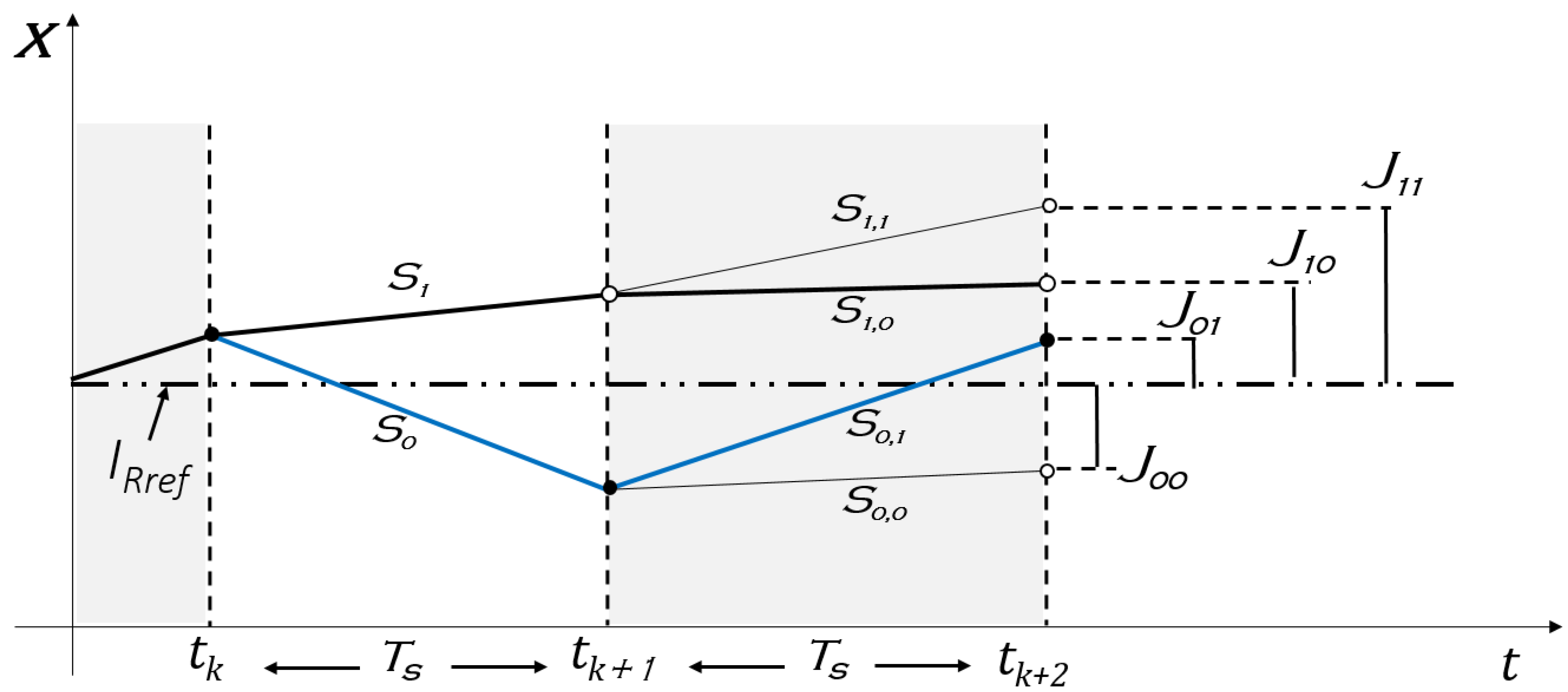
In this work, an MPC with a prediction horizon equal to two $h=2$ is used. To this end, the calculation of the controlled variable $I_L$ at time $t_{k+2}$ is necessary. However, this could be an easy task by using Equations (13) and (14). The process of the proposed MPC technique with a prediction horizon $h=2$ is depicted in Figure 5. According to this figure, to calculate the value of the predicted controlled variable $I_{L(k+2)}$, the calculation of the system variables at time $t_{k+1}$ is required.

Figure 6 illustrates the operating principle of the proposed MPC technique. Hence, by observing the system behavior for the future two-step horizon and by evaluating the cost function at each step, it will be possible to select the best switching state at which the cost function has the lowest value. All the possible sets of switching states that could be evaluated for $h=2$ are given in Equation (15).

$$\left\{\begin{array}{c}{S}_{(k+1)}=0and{S}_{(k+2)}=0\hfill \\ \hfill & \\ S_{(k+1)}=0and{S}_{(k+2)}=1\hfill \\ \hfill & \\ S_{(k+1)}=1and{S}_{(k+2)}=0\hfill \\ \hfill & \\ S_{(k+1)}=1and{S}_{(k+2)}=1\hfill \end{array}\right.$$

(15)

It should be noted that there are two strategies that could be used to calculate the predicted state $X(k+2)$:

• The first one is to evaluate the cost function at each step (sampling time). For instance, by taking the example presented in Figure 6 where the performed switching actions are indicated with the bold black line; at first, when the sampling time is $t_k$, the controller has to choose between $S_1$ and $S_0$, where the choice is based on the most preferred switching condition that leads to minimizing the cost function J. Since $S_1$ is selected in this example, it means that the predicted controlled variable $I_{L,s=1(k+1)}$ that corresponds to $S_1$ is the closest to the desired reference $I_{ref}$. Following the same criterion for the two-step horizon at which the sampling time is $t_{k+1}$, the controller will decide between $S_{11}$ and $S_{10}$. Since $S_{10}$ is selected, then, the cost function $J_{10}$ is performed and considered as the cost function of the previous step at the sampling time $t_{k+1}$. However, despite the simplicity of this strategy, it may fall in a local lower cost function since the cost functions $J_{01}$ and $J_{11}$ that, respectively, correspond to the switching states $S_{01}$ and $S_{11}$, were not evaluated.
• The second strategy is to evaluate the cost functions of all the sets of switching states given in Equation (15), and finally, the lowest cost function is performed. The performed switching actions using this method are indicated with the bold blue line. The main feature of this method is its capability to calculate the global lower cost function for the two-step horizon. Therefore, a new cost function for the two-step prediction horizon is defined in Equation (16). The latter is composed of the error at the sampling time $t_{k+1}$ plus the error at the sampling time $t_{k+2}$.

  $$J_{s=m}^{n=0,1\&m=0,1}=|I_{L,s=m(k+2)}-I_{ref}|+J_{s=n}$$

  (16)

The evaluation of the four cost functions $J_{00}$, $J_{01}$, $J_{10}$ and $J_{11}$, for the two-step horizon is presented in Figure 7. The combination with the lower cost function value for the two-step prediction horizon is represented by the black color, where faded colors were used for the combinations with higher cost function values. According to these combinations, if the first method of prediction is used, the preferred cost function belongs to Combination 3 since $S_1$<$S_0$ and $S_{10}$<$S_{11}$. If we only consider the evaluation of the cost function for the one-step (Equation (12)), the preferred cost function belongs to Combination 3 or 4 since $S_1$<$S_0$. If we only consider the evaluation of the cost function for the two-step ($J_{s=m}^{m=0,1}$), the preferred cost function belongs to Combination 2 since $S_{01}$ is lower than $S_{00}$, $S_{10}$ and $S_{11}$. However, although this evaluation gives the same result as the proposed method for the example presented in Figure 7, it may not be the most appropriate for other examples. Therefore, a combined cost function involving the two steps, as defined in Equation (16), can provide the best switching condition for tracking the desired reference.

2.3. Performance Metrics Used

To achieve the best performance, the gains of the controller were obtained through the minimization of the integral of the absolute error (IAE), which is given in Equation (17). This helps to adjust the controller parameters through a decrement in the tracking error in real-time.

$$IAE=\sum _{i=1}^N\left|e_i\right|\Delta t$$

(17)

where $e_i$ is the tracking error and N is an observation data length time for the calculation.

Since the main objective of this research is the tracking performance enhancement, not only was the IAE calculated but other types of metrics were also used to gather accurate results. These were the root-mean-square-error (RMSE) and the relative root-mean-square (RRMSE), which are reflected in Equations (18) and (19), respectively, where $r_i$ is the reference along the i-th sample.

$$RMSE=\sqrt{{\displaystyle \frac{1}{N}}\sum _{i=1}^N{\left(e_i\right)}^2}$$

(18)

$$RRMSE=\sqrt{\sum _{i=1}^N{\left(e_i\right)}^2/\sum _{i=1}^N\left(r_i\right)}\times 100\%$$

(19)

3. Results

Figure 8 tackles the response behavior of the stack current signal under the application of the proposed MPC method and the classical PI control. To test the performance of the controllers and their capability of counteracting the disturbance, load resistance variation is applied at two times instances $t_1=25\mathrm{s}$ and $t_2=45\mathrm{s}$. These times correspond, respectively, to resistance rising from 20 to $50\mathsf{\Omega }$ and decreasing from 50 to $20\mathsf{\Omega }$. The coefficient parameters of the PI controller were tuned through the minimization of IAE, and they are equal to 0.02 and 10 for the proportional and integral terms, respectively.

It is clear from the first load variation, depicted in Figure 8b, that the MPC approach converges rapidly to the reference current with a response time equal to $1.3\mathrm{s}$ against an important response value for the classical PI controller, which is around $6.8\mathrm{s}$. It should be noted that $0.12\mathrm{s}$ of the response time was caused by the delay time, which occurred at the moment in which the load variation was applied. Hence, the proposed MPC controller achieved a significant improvement in the convergence speed of almost $81\%$. On the other hand, the MPC presents a reduced undershoot equal to $1.73\mathrm{A}$ compared with the conventional PI method, which is around $2.1\mathrm{A}$. Consequently, the proposed algorithm can effectively reduce the undershoot with an enhancement of $17.61\%$ compared with the PI controller.

The impact of reducing the load resistance on the response of the stack current is illustrated through Figure 8c. It is obviously clear from this figure that the PI controller takes a significant time to reach the current reference with a response time equal to $7.25\mathrm{s}$, while only $0.51\mathrm{s}$ is obtained via the proposed MPC, which effectively outperforms the convergence speed of the PI with $92.9\%$. According to this figure, it is noticed that the current signal controlled via the proposed MPC made a delay time of $0.02\mathrm{s}$. However, this time is almost negligible, and it has no negative effect on the response time. Regarding the overshoots, a significant one of almost $3.65\mathrm{A}$ is shown on the response behavior of the conventional PI, while an improvement of around $13.69\%$ on the overshoot is obtained using the proposed MPC method.

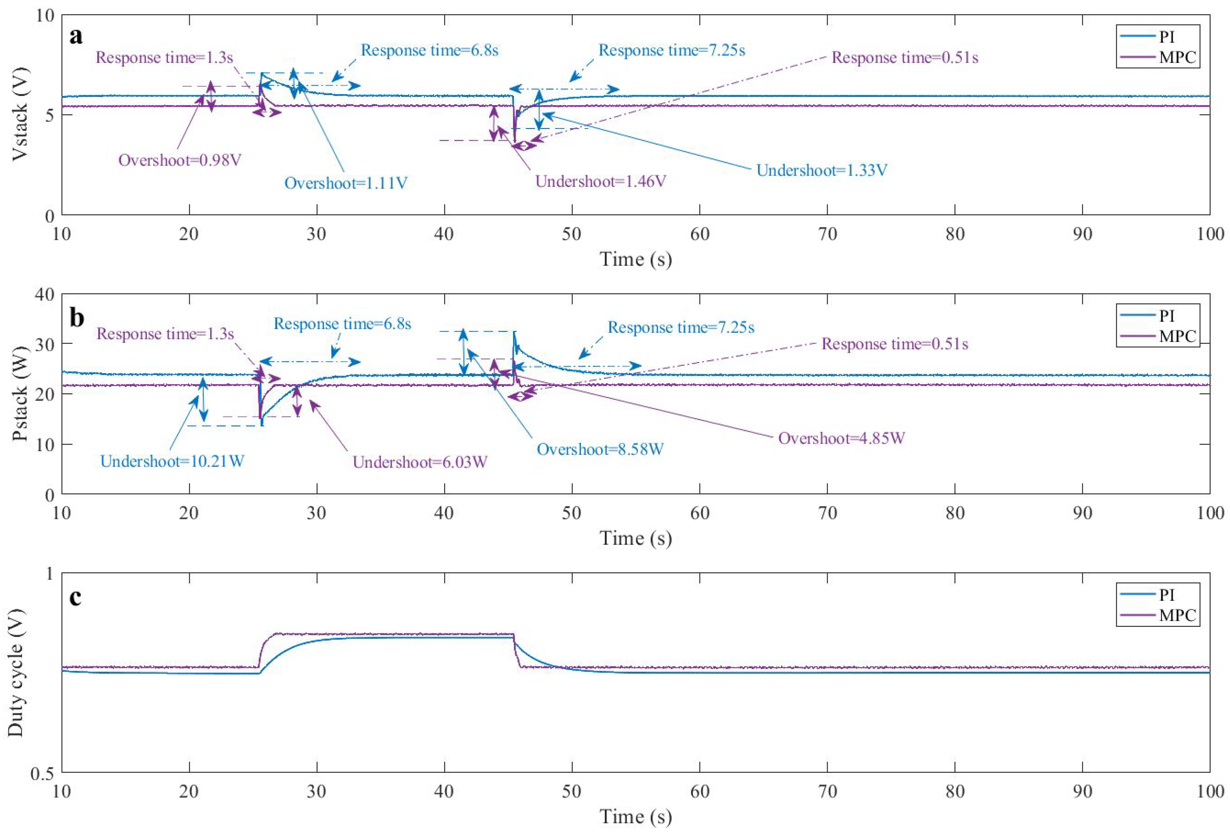
Figure 9a–c illustrates, respectively, the real-time response of the PEMFC voltage, power and duty cycle delivered by the classical PI and the proposed MPC approach. The slight variation between the experimental test of the PI and MPC that appeared in a,b and c occurred due to the effect of the operating temperature on the membrane since it is difficult to carry out two experiments at exactly the same temperature. It should be noted that this variation did not appear in the graphs of the stack current (Figure 8) since it is a controlled signal where both of the algorithms drive the stack current to operate at the same reference current $I_{ref}$.

According to Figure 9a, the effectiveness of the proposed MPC algorithm over the conventional PI appears to reduce the overshoots and undershoots of the stack voltage. Thus, the PI controller presents a voltage value around $1.11\mathrm{V}$ and $1.33\mathrm{V}$ for the first and the second load variation, respectively. On the other hand, the proposed MPC shows values of $0.98\mathrm{V}$ and $1.46\mathrm{V}$ for the same load variations.

From Figure 9b, it can be seen that the proposed MPC method effectively tracks the desired output power of the PEMFC with an almost negligible ripple around the steady state. Moreover, in comparison with the conventional PI controller, the results show that a reduction of $4.18\mathrm{W}$ and $3.73\mathrm{W}$ in the undershoot and overshoot are obtained for the first and the second load variation, respectively.

The real-time responses of the output current, voltage and power for the DC–DC boost converter are depicted in Figure 10a–c. The latter clearly shows the impact of the variable load resistance on the response behavior of the output current and the output voltage for the two controllers. Furthermore, the slow converging and high overshoots of the PI controller in comparison with the proposed MPC are clearly presented in this figure.

Finally, it is clearly demonstrated in the above results that the proposed MPC has succeeded in overcoming the drawbacks of the conventional PI controller. Hence, a robust and fast response, as well as better dynamic behavior when facing large load variation, are obtained via the application of the proposed MPC method.

Performance Metrics Comparison

To obtain high control performance, the error signal should be reduced so as to improve the tracking accuracy. Consequently, the IAE was minimized by tuning the corresponding gains, and therefore, the metrics in terms of error were determined during a period of two load variations.

Table 4. Comparison of the different metrics.

IAE		RMSE		RRMSE (%)
MPC	PI	MPC	PI	MPC	PI
2.0607	9.2310	0.2068	0.5085	5.1705	12.7115

enlists the obtained values of the IAE, RMSE and RRMSE for both controllers.

According to this table, the IAE revealed an expected improvement for the proposed MPC where the conventional PI showed a value of 4.48 times higher than the proposed controller. Regarding the RMSE, the reflection is similar for the same period. The MPC yields an RMSE of 0.2068, whereas the PI downgraded the performance to 0.5085, which implies a difference of 2.46 times. Finally, the RRMSE endures the previous trend where the proposed MPC overcame the comparisons. Hence, the PI showed a value of 12.7%, whereas the MPC diminished up to 5.17%, resembled by a 2.45-times difference.

4. Conclusions

The purpose of this paper was to improve the performance of the PEM fuel cell system via the application of a predictive module controller (MPC). The proposed controller scheme was designed based on a global minimum cost function for a two-step horizon in order to enhance the efficiency and the convergence tracking speed of the power delivered by the PEM fuel cell system.

A real-time implementation of the MPC method compared with a PI controller was realized to reveal the advantages of this proposed approach, where the robustness was tested via the application of large load variation through an advanced electronic variable resistance device.

Experimental results have clearly demonstrated the effectiveness of the proposed MPC method over the conventional PI controller. The latter showed an undershoot of $2.1\mathrm{A}$, an overshoot of $3.65\mathrm{A}$, and a response time of 6.8 and $7.25\mathrm{s}$, respectively, for the first and second load variation. On the other hand, results of the proposed MPC showed an undershoot of $1.73\mathrm{A}$, an overshoot of $3.15\mathrm{A}$, and a response time of 1.3 and $0.51\mathrm{s}$, respectively, for the same first and second load variation applied to the PI controller. Hence, the controlled stack current signal has achieved significant improvement in the convergence speed with an average value of $86.9\%$ and a reduced overshoot around $15.65\%$. Therefore, high tracking accuracy with a fast and robust response as well as global stability of the closed-loop system are obtained via the application of the proposed MPC method.

Finally, the experimental results obtained in this work are quite encouraging, and they pave the way for further advanced research in the performance improvement of PEM fuel cell systems.

References

- Magoon, C.R., Jr. Creation and the Big Bang: How God Created Matter from Nothing; WestBow Press: Edinburgh, UK, 2018. [Google Scholar]
- Choudhury, D.; Kraft, D.W. Big Bang Nucleosynthesis and the Missing Hydrogen Mass in the Universe. AIP Conf. Proc. 2004, 698, 345–348. [Google Scholar]
- Derbeli, M.; Farhat, M.; Barambones, O.; Sbita, L. Control of PEM fuel cell power system using sliding mode and super-twisting algorithms. Int. J. Hydrogen Energy 2017, 42, 8833–8844. [Google Scholar] [CrossRef]
- Thounthong, P.; Mungporn, P.; Pierfederici, S.; Guilbert, D.; Bizon, N. Adaptive Control of Fuel Cell Converter Based on a New Hamiltonian Energy Function for Stabilizing the DC Bus in DC Microgrid Applications. Mathematics 2020, 8, 2035. [Google Scholar] [CrossRef]
- Bizon, N.; Thounthong, P. A Simple and Safe Strategy for Improving the Fuel Economy of a Fuel Cell Vehicle. Mathematics 2021, 9, 604. [Google Scholar] [CrossRef]
- Bizon, N.; Thounthong, P. Energy efficiency and fuel economy of a fuel cell/renewable energy sources hybrid power system with the load-following control of the fueling regulators. Mathematics 2020, 8, 151. [Google Scholar] [CrossRef] [Green Version]
- Bahrami, M.; Martin, J.P.; Maranzana, G.; Pierfederici, S.; Weber, M.; Meibody-Tabar, F.; Zandi, M. Multi-stack lifetime improvement through adapted power electronic architecture in a fuel cell hybrid system. Mathematics 2020, 8, 739. [Google Scholar] [CrossRef]
- Derbeli, M.; Farhat, M.; Barambones, O.; Sbita, L. Control of proton exchange membrane fuel cell (pemfc) power system using pi controller. In Proceedings of the IEEE 2017 International Conference on Green Energy Conversion Systems (GECS), Hammamet, Tunisia, 23–25 March 2017; pp. 1–5. [Google Scholar]
- Rubio, J.D.J.; Bravo, A.G. Optimal control of a PEM fuel cell for the inputs minimization. Math. Probl. Eng. 2014, 2014. [Google Scholar] [CrossRef]
- Belhaj, F.Z.; El Fadil, H.; Idrissi, Z.E.; Koundi, M.; Gaouzi, K. Modeling, Analysis and Experimental Validation of the Fuel Cell Association with DC-DC Power Converters with Robust and Anti-Windup PID Controller Design. Electronics 2020, 9, 1889. [Google Scholar] [CrossRef]
- Qi, Z.; Tang, J.; Pei, J.; Shan, L. Fractional controller design of a DC-DC converter for PEMFC. IEEE Access 2020, 8, 120134–120144. [Google Scholar] [CrossRef]
- Fathy, A.; Abdelkareem, M.A.; Olabi, A.; Rezk, H. A novel strategy based on salp swarm algorithm for extracting the maximum power of proton exchange membrane fuel cell. Int. J. Hydrogen Energy 2021, 46, 6087–6099. [Google Scholar] [CrossRef]
- Derbeli, M.; Sbita, L.; Farhat, M.; Barambones, O. Proton exchange membrane fuel cell—A smart drive algorithm. In Proceedings of the IEEE 2017 International Conference on Green Energy Conversion Systems (GECS), Hammamet, Tunisia, 23–25 March 2017; pp. 1–5. [Google Scholar]
- Luta, D.N.; Raji, A.K. Fuzzy rule-based and particle swarm optimisation MPPT techniques for a fuel cell stack. Energies 2019, 12, 936. [Google Scholar] [CrossRef] [Green Version]
- Reddy, K.J.; Sudhakar, N. ANFIS-MPPT control algorithm for a PEMFC system used in electric vehicle applications. Int. J. Hydrogen Energy 2019, 44, 15355–15369. [Google Scholar] [CrossRef]
- Reddy, K.J.; Sudhakar, N. High voltage gain interleaved boost converter with neural network based MPPT controller for fuel cell based electric vehicle applications. IEEE Access 2018, 6, 3899–3908. [Google Scholar] [CrossRef]
- Chorfi, J.; Zazi, M.; Mansori, M. A new intelligent MPPT based on ANN algorithm for photovoltaic system. In Proceedings of the IEEE 2018 6th International Renewable and Sustainable Energy Conference (IRSEC), Rabat, Morocco, 5–8 December 2018; pp. 1–6. [Google Scholar]
- Hadji, S.; Gaubert, J.P.; Krim, F. Real-time genetic algorithms-based MPPT: Study and comparison (theoretical an experimental) with conventional methods. Energies 2018, 11, 459. [Google Scholar] [CrossRef] [Green Version]
- Khanam, N.; Khan, B.H.; Imtiaz, T. Maximum Power Extraction of Solar PV System using Meta-Heuristic MPPT techniques: A Comparative Study. In Proceedings of the IEEE 2019 International Conference on Electrical, Electronics and Computer Engineering (UPCON), Aligarh, India, 8–10 November 2019; pp. 1–6. [Google Scholar]
- Derbeli, M.; Barambones, O.; Farhat, M.; Sbita, L. Efficiency Boosting for Proton Exchange Membrane Fuel Cell Power System Using New MPPT Method. In Proceedings of the IEEE 2019 10th International Renewable Energy Congress (IREC), Sousse, Tunisia, 26–28 March 2019; pp. 1–4. [Google Scholar]
- Derbeli, M.; Barambones, O.; Ramos-Hernanz, J.A.; Sbita, L. Real-time implementation of a super twisting algorithm for PEM fuel cell power system. Energies 2019, 12, 1594. [Google Scholar] [CrossRef] [Green Version]
- Silaa, M.Y.; Derbeli, M.; Barambones, O.; Napole, C.; Cheknane, A.; Gonzalez De Durana, J.M. An Efficient and Robust Current Control for Polymer Electrolyte Membrane Fuel Cell Power System. Sustainability 2021, 13, 2360. [Google Scholar] [CrossRef]
- Derbeli, M.; Barambones, O.; Sbita, L. A robust maximum power point tracking control method for a PEM fuel cell power system. Appl. Sci. 2018, 8, 2449. [Google Scholar] [CrossRef] [Green Version]
- Derbeli, M.; Barambones, O.; Farhat, M.; Ramos-Hernanz, J.A.; Sbita, L. Robust high order sliding mode control for performance improvement of PEM fuel cell power systems. Int. J. Hydrogen Energy 2020, 45, 29222–29234. [Google Scholar] [CrossRef]
- Derbeli, M.; Barambones, O.; Silaa, M.Y.; Napole, C. Real-Time Implementation of a New MPPT Control Method for a DC-DC Boost Converter Used in a PEM Fuel Cell Power System. Actuators 2020, 9, 105. [Google Scholar] [CrossRef]
- Silaa, M.Y.; Derbeli, M.; Barambones, O.; Cheknane, A. Design and Implementation of High Order Sliding Mode Control for PEMFC Power System. Energies 2020, 13, 4317. [Google Scholar] [CrossRef]
- Lashab, A.; Sera, D.; Guerrero, J.M. A dual-discrete model predictive control-based MPPT for PV systems. IEEE Trans. Power Electr. 2019, 34, 9686–9697. [Google Scholar] [CrossRef]
- Güler, N.; Irmak, E. MPPT Based Model Predictive Control of Grid Connected Inverter for PV Systems. In Proceedings of the 2019 8th International Conference on Renewable Energy Research and Applications (ICRERA), Brasov, Romania, 3–6 November 2019; pp. 982–986. [Google Scholar]
- Golzari, S.; Rashidi, F.; Farahani, H.F. A Lyapunov function based model predictive control for three phase grid connected photovoltaic converters. Solar Energy 2019, 181, 222–233. [Google Scholar] [CrossRef]
- Ahmed, M.; Abdelrahem, M.; Kennel, R. Highly Efficient and Robust Grid Connected Photovoltaic System Based Model Predictive Control with Kalman Filtering Capability. Sustainability 2020, 12, 4542. [Google Scholar] [CrossRef]
- Irmak, E.; Güler, N. A model predictive control-based hybrid MPPT method for boost converters. Int. J. Electr. 2020, 107, 1–16. [Google Scholar] [CrossRef]
- Abdel-Rahim, O.; Wang, H. A new high gain DC-DC converter with model-predictive-control based MPPT technique for photovoltaic systems. CPSS Trans. Power Electr. Appl. 2020, 5, 191–200. [Google Scholar] [CrossRef]
- Xue, D.; El-Farra, N.H. Forecast-triggered model predictive control of constrained nonlinear processes with control actuator faults. Mathematics 2018, 6, 104. [Google Scholar] [CrossRef] [Green Version]
- Wong, W.C.; Chee, E.; Li, J.; Wang, X. Recurrent neural network-based model predictive control for continuous pharmaceutical manufacturing. Mathematics 2018, 6, 242. [Google Scholar] [CrossRef] [Green Version]
- Zhang, Z.; Wu, Z.; Rincon, D.; Christofides, P.D. Real-time optimization and control of nonlinear processes using machine learning. Mathematics 2019, 7, 890. [Google Scholar] [CrossRef] [Green Version]
- Durand, H. Responsive economic model predictive control for next-generation manufacturing. Mathematics 2020, 8, 259. [Google Scholar] [CrossRef] [Green Version]
- Banholzer, S.; Fabrini, G.; Grüne, L.; Volkwein, S. Multiobjective model predictive control of a parabolic advection-diffusion-reaction equation. Mathematics 2020, 8, 777. [Google Scholar] [CrossRef]
- Aziz, A.G.M.A.; Rez, H.; Diab, A.A.Z. Robust Sensorless Model-Predictive Torque Flux Control for High-Performance Induction Motor Drives. Mathematics 2021, 9, 403. [Google Scholar] [CrossRef]
- Rodriguez, J.; Kazmierkowski, M.P.; Espinoza, J.R.; Zanchetta, P.; Abu-Rub, H.; Young, H.A.; Rojas, C.A. State of the Art of Finite Control Set Model Predictive Control in Power Electronics. IEEE Trans. Ind. Inform. 2013, 9, 1003–1016. [Google Scholar] [CrossRef]
- Rodriguez, J.; Cortes, P. Predictive Control of Power Converters and Electrical Drives; John Wiley & Sons: Hoboken, NJ, USA, 2012; Volume 40. [Google Scholar]
- Bououden, S.; Hazil, O.; Filali, S.; Chadli, M. Modelling and model predictive control of a DC-DC Boost converter. In Proceedings of the IEEE 2014 15th International Conference on Sciences and Techniques of Automatic Control and Computer Engineering (STA), Hammamet, Tunisia, 21–23 December 2014; pp. 643–648. [Google Scholar]
Figure 1.
Overview of the experimental test bench.
Figure 2.
Basic concept for model predictive control (MPC).
Figure 3.
MPC scheme for power electronic converters.
Figure 4.
Block scheme of the proposed MPC technique.
Figure 5.
Schematic diagram of the proposed MPC process with a 2-step prediction horizon.
Figure 6.
Schematic diagram of the proposed MPC operating principle.
Figure 7.
Schematic diagram of the switching condition combinations for the 2-step horizon and the evaluation of the respective cost functions.
Figure 8.
(a) Stack current signal; (b) stack current behavior when increasing the load resistance; (c) stack current behavior when decreasing the load resistance; (d) steady state.
Figure 9.
(a) PEMFC stack voltage signal; (b) PEMFC stack power; (c) duty cycle signal.
Figure 10.
(a) DC–DC output current signal; (b) DC–DC output voltage signal; (c) DC–DC output power signal.