
Development of an Intelligent Decision Support System for Attaining Sustainable Growth within a Life Insurance Company


1
School of Water, Energy and Environment, Cranfield University, Cranfield MK43 0AL, UK
2
Department of Agricultural Economics and Business Management, Aligarh Muslim University, Aligarh 202002, India
3
Department of Computer Information Systems, Middle East University, Amman 11831, Jordan
4
Department of Medical Research, China Medical University Hospital, China Medical University (Taiwan), Taichung 40402, Taiwan
*
Author to whom correspondence should be addressed.
†
These authors contributed equally to this work.
Mathematics 2021, 9(12), 1369; https://doi.org/10.3390/math9121369
Submission received: 18 April 2021
/
Revised: 18 May 2021
/
Accepted: 25 May 2021
/
Published: 12 June 2021
(This article belongs to the Special Issue Applications of Quantitative Methods in Business and Economics Research)
Abstract
:Consumer behaviour is one of the most important and complex areas of research. It acknowledges the buying behaviour of consumer clusters towards any product, such as life insurance policies. Among various factors, the three most well-known determinants on which human conjecture depends for preferring a product are demographic, economic and psychographic factors, which can help in developing an accurate market design and strategy for the sustainable growth of a company. In this paper, the study of customer satisfaction with regard to a life insurance company is presented, which focused on comparing artificial intelligence-based, data-driven approaches to classical market segmentation approaches. In this work, an artificial intelligence-based decision support system was developed which utilises the aforementioned factors for the accurate classification of potential buyers. The novelty of this paper lies in developing supervised machine learning models that have a tendency to accurately identify the cluster of potential buyers with the help of demographic, economic and psychographic factors. By considering a combination of the factors that are related to the demographic, economic and psychographic elements, the proposed support vector machine model and logistic regression model-based decision support systems were able to identify the cluster of potential buyers with collective accuracies of 98.82% and 89.20%, respectively. The substantial accuracy of a support vector machine model would be helpful for a life insurance company which needs a decision support system for targeting potential customers and sustaining its share within the market.
1. Introduction
The sustainable growth of a company is considered a significant target which involves focusing on service strategies and operations which can efficiently satisfy the needs of customers [1]. It is well established that in order to sustain the interest of and utility to a consumer, it is critically important that the choice of product is to be judged on the basis of its quality, reputation, price, etc. [2].
When consumers need a specific product, they usually search for a large variety of similar products and try to evaluate those variants in order to discover the best product which might satisfy their needs in the best possible manner. The behaviour displayed by the consumer in the complete selection process is termed consumer behaviour [3]. The above scenario asserts that consumer behaviour is a systematic process which involves different activities, and the consequence of the process is the main step which influences the consumer in a definite way.
According to Solomon [4], consumer behaviour includes the processes of selection, purchasing, use and disposal for services, ideas or experiences. A similar theory was also suggested by Hawkins and Mothersbaugh [5], which states that consumer behaviour involves the study of satisfaction during the process adopted by a buyer, group of buyers or organisation while the choosing, securing and disposing of a product, service or experience. These analogous definitions have established that consumer behaviour is a specific process in which consumers decide to expend the resources they possess, such as money, effort and time, on objects for their consumption.
It can be noted that the consumer behaviour process has three stages [6]. The first stage is the process where the consumer makes a decision to buy a product; it is the longest and most complex stage, as it involves various factors all playing important roles. The second stage is the one in which the consumer purchases the product; this stage depicts the choice and final decision. The third stage constitutes the usage and disposal of the product; at this stage, the customer’s satisfaction is revealed, and sustainable consumer loyalty is created only if the product efficiently meets the desirable requirements. That is, in the third stage, if the consumer is satisfied with the product, then in the future they will be more in favour of purchasing the same product.
Although human perceptions of any product depend on the quality, price and marketing of the product, there are various other elements which also influence their buying behaviour. Examples include demographic, economic and psychographic factors of the consumer [7]. Hence, it is vital to investigate the roles of such factors in the orientation of consumer behaviour towards any product. It is worth noting that analysing the orientations of such factors is helpful for developing a sustainable market design and strategy.
The core objectives of this study were analysing the dissimilarities in the demographic, economic and psychographic factors among clusters of buyers and non-buyers of life insurance in India, and developing artificial intelligence models for classifying the clusters via dissimilarities. The life insurance penetration of India decreased from 3.10% in 2013 to 2.76% in 2017 [8], which has impacted the domestic economy of the country [9]. Over the years, the life insurance sector has grown in India, in which the IRDA has played a prominent role. The life insurance market in India is growing at good pace, however, 50% of the insurable population is still not covered by life insurance. Hence, there is a vast scope for life insurance in India [10].
Based on the current situation of the life insurance market in India, it can be asserted that accurately targeting customers with the help of a machine learning-based decision support system would help a given insurance company to quickly expand and sustain its market share [11,12]. Hence, this paper focused on estimating the cluster of consumers who opt for life insurance policies. These were classified with well-known factors, such as demographic factors, economic factors and psychographic factors. Additionally, this paper has given emphasis to developing an efficient supervised machine learning model for finding potential Indian customers of life insurance with the help of the aforementioned factors. These customers can be targeted by life insurance companies to elevate life insurance’s penetration rate, and ensure sustainable growth.
Researchers have found that consumers possess certain kinds of similarities in their considerations, but still differ a lot in how they favour products according to their preferences and needs [13]. Hence, consumer behaviour is very diverse, because every consumer has different preferences based on their opinions, personality, etc. Therefore, the prediction of the behaviour of consumers is one of the challenging tasks facing researchers [14,15]. The diversification of products and the globalisation of the market have undoubtedly contributed to expanding the product market, but have further complicated consumer behaviour. In this context, supervised machine-learning-based decision support systems are likely to play a crucial role in classifying complex behaviours [16]. Notably, artificial intelligence systems can be seen as advanced forms of multicriteria decision-making systems that do not require too much in-depth analysis or user-based knowledge of their target scenarios to reach optimal solutions [17,18]. During the learning process, unlike fuzzy-based multicriteria decision-making systems, artificial intelligence systems automatically analyse the relationships in the dataset and provide weights to the features, which are relevant for escalating the accuracy of the classification process.
The concept of market segmentation is one of the solutions to forecast the unpredictable behaviour of the consumers [19]. In the market segmentation, the heterogeneous market is divided into exclusive homogenous sections which contain features like income group or age group, etc., through which the consumers can be targeted by a company via formulating a marketing-blend technique [3]. However, due to the advancement of data-driven artificial intelligence approaches, the forecasting of consumer behaviour has made a new leap. A blend of powerful statistical analysis tools and machine learning approaches can help highlight the core determinants for advancing the concept of consumer behaviour.
Hence, this paper proposes a supervised machine learning modelling approach to conducting advanced consumer behaviour research. One of the initial and essential parts of consumer behaviour research is the collection of primary responses from the consumers/buyers of a life insurance policy, which should be analysed by categorising into different groups, such as the effect of income categories on buying pattern, the effect of age on buying behaviour. The novelty of this study lies in investigating the core determinants that tend to influence the buying behaviour of a life insurance policy through statistical analysis, and utilise these determinants for developing a supervised machine learning-based decision support system which can target the potential customers.
The remainder of the paper is organised as follows. The instructive overview of materials and methods is described in Section 2. The core elements associated with the buying behaviour of a life insurance product is discussed in detail in Section 3. The simulation results are discussed in Section 4, followed by concluding remarks in Section 5.
2. Materials and Methods
The main objective of the study is to develop a supervised machine learning-based decision support system by understanding the various external and internal influential factors of the policyholder while buying a life insurance policy. To achieve this objective, a literature survey has been conducted to estimate the major behavioural factors, and the questionnaire has been designed for primary data collection from three Indian cities, which is given in Supplementary Table S1. In this study, three cities, namely Delhi (NCR), Lucknow and Aligarh, having approximate populations of 46.90 million, 2.81 million, 0.87 million, respectively, [20], were chosen for data collection.
In order to achieve the aforementioned goal, the investigation was divided into the following sub-objectives:
- Identifying the major determinants affecting the buying behaviour of a life insurance policy through a literature survey;
- Creating a questionnaire for primary data collection;
- Targeting the Indian cities for data collection;
- Distinguishing the dissimilarities in the factors between buyers and non-buyers of a life insurance policy;
- Utilising the statistically significant core factors as features for supervising the machine learning algorithms for the classification process;
- Finally, developing an intelligent decision support system that utilises logistic regression and support vector machine (SVM) algorithms to accurately classify the potential buyers.
3. Core Elements Associated with Buying Behaviour of Life Insurance Product
The major determinants through which the buying behaviour of life insurance products can be investigated are broadly classified in the domain of demographic, economic and psychographic factors [21,22]. In this section, the importance of each factor is discussed and the determinants/sub-factors are differentiated into positive or negative manners.
3.1. Demographic Factors
The demographic factors are the particular features of a population which help in categorising them on the basis of age, gender, education level, income level, marital status and occupation.
3.1.1. Age
Truett and Truett [23] have found a positive relation between age and life insurance demand within the age group of 25–64 years. The individuals of the age group lying in the range of 25–64 years want to secure the future of their dependents from unfortunate events such as the death of the sole earning member of the family. Other studies have also shown a similar positive effect of the age factor on life insurance demand [24,25,26].
The study conducted by Yusuf et al. [27] has estimated the buying behaviour of Nigerians and found that age has a positive effect on demand for life insurance. The investigations through ANOVA and employing least significant difference (LSD) tests show that there is a lower extent of positive behaviour for life insurance demand among the respondents lying in the age group up to 45 years, while the greatest demand is from respondents residing in the age group of 56–65 years. The cause of a positive effect in demand is due to the increase in age that would make them more conscious about the future, and hence, try to secure their post-retirement future with the help of life insurance policy.
A novel understanding of life insurance demand has been proposed by Chen et. al by merging the perspective of age, period and cohort effects. It has been suggested that the separation of the age, period, and cohort effects can precisely forecast the future life insurance demand [28]. While Bernheim [29] has estimated the existence of a relation between the wish to leave bequest and life insurance demand, it was also found that a substantial amount of savings of the retired individual is likely to be invested in life insurance. The study conducted on longitudinal data of retired individuals lying in the age group of 64–69 years has revealed that the demand for life insurance reduces as age increases, which asserts that after a certain age, individuals restrict themselves from future savings.
Unlike others, Gandolfi and Laurence [30], Burnett and Palmer [31], Duker [32], Hammond et al. [33] have pointed out that there are no associations between age and demand for life insurance. Among these, Gandolfi and Laurence have studied the demand for life insurance on the basis of the gender of the married individuals and found that the age of the husbands showed a negative relation to the life insurance demand, whereas the age of the wives had no relation or association with the demand for life insurance [30].
3.1.2. Education
According to Truett and Truett [23], highly educated people buy life insurance more frequently compared to less educated persons likely because they are more aware of insurance products, and they can easily analyse and compare different types of life insurance products. Furthermore, educated individuals want their dependents to be secure against risk compared to uneducated ones [23]. Some of the studies have asserted that there is a positive relationship between education and the demand for life insurance [23,24,31,34,35,36,37,38,39,40,41,42,43]. The positive attitude of educated people toward life insurance shows that they are more conscious about uncertainties in life, and hence tend to buy life insurance to averse the risk of an unfortunate event [43].
In contrast, Anderson and Nevin [44] conducted a similar study through multiple classification analysis to find the factors which influence a newly married couple to buy life insurance. The results depict the negative relationship, i.e., a higher number of insurances were bought by a less-educated husband because of low income. Hence, life insurance acts as a source of income for the future of less-educated husbands.
3.1.3. Employment Status
Employment status is another sub-factor that positively affects the demand for life insurance, because employed people usually receive continuous income so they can buy life insurance, whereas unemployed persons cannot buy it because of the lack of income source [45,46]. Likewise, a higher level of employment signifies high status and awareness about life insurance, hence they show more concern towards protecting the future of their family members. Hence, it can be stated that there is a positive relation between employment and life insurance demand [39,45,46].
Similarly, Yusuf, Gbadamosi and Hamadu [27] also found a positive association between the employment status of respondents and their buying attitude for a life insurance policy. Furthermore, it has been found that the respondents who had retired from their job showed a positive behaviour towards life insurance equal to that shown by employed respondents. Furthermore, a higher positive association between employment and life insurance is found in self-employed respondents compared to the students or part-time employed individuals.
In contrast, the study by Gandolfi and Miner [30] has proved a negative association between employment and life insurance demand, because when both husband and wife are employed, they feel more secure so they might have less willingness to buy a life insurance product. In contrast, the study by Baek and DeVaney [47] showed that if both husband and wife are employed, then more income is generated in the family, which will lead to a greater chance of buying a life insurance policy.
3.1.4. Gender
Gandolfi and Miners [30] investigated the variation in the demand for life insurance on a gender basis and found that the consumption behaviour of life insurance is largely dependent on gender. They also indicated that age, possession of a home, and the size of the family also act as crucial variables for depicting the demand for life insurance in men and women. Similarly, Curak, Dzaja and Pepur [48] and Sharma [49] found no association between the demand for the life insurance and gender of the respondent, hence concluding that both men and women equally buy life insurance policy.
In contrast, the study conducted by Tati and Baltazar [37] showed that there is variation among the opinions of men and women regarding life insurance, and comparatively, men hold more positive opinions than women.
3.1.5. Number of Dependents
Some studies proved a positive relation between the number of dependents and the demand for life insurance [40,43,50]. It was also observed that as the number of dependents increases, the individual is more willing to secure their future and hence more likely to spend more on life insurance [43,51].
While Curak et al. [48] in their study found that a large portion of respondents have one dependent, and that life insurance purchase is equal among the respondents having one dependent, while it is less among the respondents having two or more than two dependents, which asserted that the number of dependents and demand for life insurance are not associated with each other.
3.1.6. Marital Status
The role of marriage or civil partnership is also deemed as one of the crucial demographic factors through which association with the buying behaviour of life insurance can be estimated [38]. Mantis and Farmer [46] used multiple regression to forecast the demand for life insurance by married people. The study showed that there is a negative relationship between life insurance premium expenditure and marital status.
A study conducted by Anderson and Nevin [44] on the buying behaviour of young married couples of life insurance policy has revealed that recently married couples are likely to buy a life insurance policy when their net assets are high or when the wife already possess a life insurance policy prior to the marriage.
Royne [52] investigated the impact of the marital status of respondents on the procedure of making a decision of whether to opt for certain services. The services that were included in the questionnaire were vacation travel, life insurance, child’s school and restaurant. Only married women were included in the study to mitigate the impact of the gender factor and they were asked about the decision-maker for each service. The results showed that for taking the decision about life insurance, the husband is the leading decision maker.
Curak et al. [48] study showed that from the total sample of 95 respondents from Croatia, the married respondents’ count was 56, while that of unmarried respondents was 39. The analysis showed that there is no association between the marital status of the respondent and the demand for life insurance policy.
3.2. Economic Factors
Economic factors are divided into various sub-factors, namely income, personal savings and wealth, inflation, and taxation. The impact of these sub-factors on life insurance demand is examined in the sub-sections.
3.2.1. Income
Generally, in developing counties, the family relies on a single earning member. If the sole earner of a family dies prematurely, then the dependents are likely to experience a financial crisis. Therefore, in this case, there is a need for life insurance which can help in coping with possible financial risk [43]. It has been observed that people with high personal disposable income are more likely to buy financial security instruments. It has been found that an increase in income raises the chances or probability to purchase a life insurance policy [23,26,31,36,37,39,40,41,43,51,53,54,55,56].
Li et al. [41] have investigated the life insurance demand in OECD countries by collecting cross-sectional data from the year 1993 to 2000. The univariate analysis shows that there is a great level of positive relation between income and life insurance acquisition, and the multivariate analysis shows that 1% increment in aggregate income results in a 0.6% increment in the sales of life insurance.
3.2.2. Saving
From various studies, it has been found that there is a negative relation between the demand for life insurance and a individual’s personal savings [53,57,58] likely due to the fact that the savings of a person act as wealth which serves as a security tool. Hence, the person does not want to buy a life insurance policy when savings are high.
Sen [59] conducted a study on 12 Asian countries and found that the demand for life insurance rises whenever there is a rise in savings because life insurance not only serves as a saving tool but also covers life risk.
Headen [60] estimated the influence of the financial portfolio of households on the demand for life insurance through a regression model, and found that the net savings have a positive and flexible effect on the demand for life insurance for a financially weaker class of the population.
3.2.3. Wealth
Fortune [56] established a negative relation between wealth and life insurance demand and the reason for such a negative relation is that as wealth increases it reduces risk-taking ability by providing a sense of financial security at the time of crises. Therefore, wealth facilitates the family to face financial loss, hence, as wealth increases, the demand for life insurance decreases [55]. In contrast, wealth can also possess a positive relation with life insurance demand because life insurance is also deemed an investment tool which gives the liquid reserve to the insured person or to the dependent [42,44,45].
The study conducted by Anderson and Nevin [44] on newly married couples revealed that the net wealth of newly married couples is one of the important elements analysing the buying behaviour of life insurance products. The higher the net wealth of newly married couples, the more likely they lean towards purchasing a life insurance policy. On the other hand, as the net wealth of newly married couples is low, they tend to buy term life insurance for the financial security of the family.
Hammond et al. [33] analysed the association between premium expenditure on life insurance and demographic and economic conditions of people through a regression model. The analyses indicate that the net wealth is positively associated with the life insurance premium expenditure, which means that life insurance does not act as a substitute for wealth and the richer families buy more life insurance policies because it provides risk cover against having to sell a property in case of an unfortunate event.
3.3. Psychographic Factors
Psychological factors include the attitude, interest, and opinion (AIO factors) of a consumer so that it can precisely understand the behaviour of a consumer. The psychographic factors are equally important with demographic and psychographic factors to obtain a clearer picture of consumer behaviour.
According to Outreville [54], more knowledgeable and educated persons tend to avoid risk so the demand for life insurance is high among them. On the other hand, according to Ferber and Lee [34], a person who invests in life insurance tends to save on a regular basis and also has an optimistic behaviour towards their future life.
3.3.1. Information, Religion and Fatalism
Karni and Zilcha [61] investigated whether the people who are more risk-averting are likely to buy more life insurance policies compared to those who are risk-takers, because life insurance ensures the payment of a fixed sum of money in the event of the death of the insured or at the end of the maturity of the policy, hence reducing the future risk.
Burnett and Palmer [31] analysed various psychographic factors to find their impact on life insurance demand by applying multiple classification analyses to find the association between psychographic variables and life insurance demand. The results show that the four main indicators of life insurance demand are socialisation, assertiveness, religion and fatalism. The investigation shows that respondents who buy more life insurance are risk-takers, not price-conscious, low information seekers, low opinion leaders, have low self-esteem, and have low brand loyalty [31,62].
Some studies indicated that information through socialisation plays a vital role for respondents, i.e., if an individual has a lesser number of people in their social group, then they will show a less social behaviour due to less diversified information. On the other hand, assertiveness is negatively related to life insurance demand, which means that respondents who do not communicate or convey themselves under conditions of stress tend to take their own decision and buy more life insurance. While considering the factors of religion and fatalism, the respondents who are not more inclined towards religion and destiny possess more life insurance.
Religious and cultural values influence the demand for life insurance as people of different countries or regions differ in terms of their cultural and religious beliefs [43,54,63]. In ancient times, it was believed that life insurance was for protecting the lives of people. Hence, life insurance was opposed by the preachers of different religions and in many European countries, and it was banned till the nineteenth century [63]. Until today, insured money or the benefiting life insurance has also been seen as unethical money which dependents obtain in exchange for the life of an insured person, hence it is considered immoral for a family to take insurance benefit [63]. Due to this reason, the life insurance demand is greater in non-Islamic countries than Islamic countries [43,54].
3.3.2. Inflation
Meko et al. [50] have found a positive relation between inflation and demand for life insurance. However, some studies indicated a negative relation between inflation and demand for life insurance [39,41,56]. Outreville [54] used the United Nations Conference on Trade and Development (UNCTAD) survey report of forty-eight countries and found a negative association between demand for life insurance and anticipated inflation. Similarly, Li et al. [41] found a negative association between life insurance demand and inflation and expected that inflation in the future tends to lower the worth of financial assets and hence lowers the demand for life insurance policy.
In contrast, some studies have found variation in the relation between the demand for life insurance and inflation [43,54,64]. For example, Hofflander and Duvall [64] have found that there are two facets of inflation that need to be studied and their impact on demand for life insurance requires thorough investigation. The two factors are income-effect and substitute-effect. The income-effect points out that as the cost of living increases with an increase in inflation, it results in a reduction in real income which ultimately reduces the demand for goods and services. As inflation increases, the premium payment for a policyholder becomes difficult, thus, the demand for life insurance decreases. In contrast, the substitute-effect explains that as inflation increases, the demand for life insurance also increases, because inflation is anticipated to further rise in the future, therefore the consumers buy more life insurance policies to secure the future of the dependents.
4. Results and Analyses
In this study, a supervised machine learning models are developed to predict the trend of the buying behaviour within three Indian cities (namely Delhi (NCR), Lucknow and Aligarh) toward the life insurance policy classified through various sub-factors lying in the domain of demographic, economic and psychographic factors. The questionnaire (referring to Supplementary Table S1) was designed based on the aforementioned sub-factors for primary data collection, and the collected data are illustrated in the form of histograms in Supplementary Figures S1–S11.
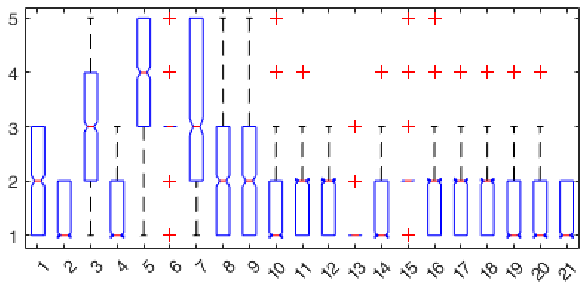
The data collected from three cities were analysed to estimate the dissimilarities in the sub-factors between buyers and non-buyers for opting for a life insurance policy. In total, 1926 people were approached in the three cities over a period of one year from December 2016 to December 2017, among which 937 responses were found to be properly filled, and hence were used as valid responses for further statistical analysis. Figure 1 illustrates the distribution of the data across 937 respondents (y axis) with respect to the response obtained through tailored questions in the questionnaire (x axis) representing demographic, economic and psychographic factors. On the other hand, Figure 2 visualises the statistical distribution of the questionnaire data (y axis) against each question (x axis) in the form of the box plot. In Figure 2, the central red coloured dash-mark within the box indicates the median value of the distribution, and the bottom and top edges of the box indicate the respective 25th and 75th percentile values, while outliers are indicated using red plus-sign. It should be noted that the objective behind analysing the dissimilarities while opting for a life insurance product is to seed only those sub-factors in the machine learning algorithms which are statistically significant for distinguishing buyers and non-buyers into two non-overlapping classes.
Notably, the supervised machine learning algorithm uses labelled data to train the model and utilises the supervised model to predict the blind data. The supervised models can be very helpful for life insurance companies through which a company can easily target a particular cluster of individuals having specific demographic/economic/psychographic features, which are likely to deliver a maximum outcome. The two supervised machine learning models that were developed in this study were SVM [65] and logistic regression [66]. Notably, the features that were chosen for developing the supervised models are the sub-factors of demographic, economic, and psychographic factors.
4.1. Support Vector Machine
SVM is a supervised discriminative classifier that uses a hyperplane to separate the feature space into two classes. In other words, given a labelled training data, the SVM algorithm finds the optimal hyperplane which can be used to predict the cluster of unknown data points. For example, in the case of consumers opting for a life insurance policy, the respondents who already have a life insurance policy is one class, while the respondents who do not have a life insurance policy is another class, then the SVM algorithms will estimate the hyperplane which can use features to efficiently discriminate between both aforementioned classes.
However, prior to modelling an SVM predictor, it is vital to analyse the feature space that is likely to be used for training the SVM model. Usually, the feature space of the clusters is comprised of the data that are not significantly different from each other; such data reduce the efficiency of the machine learning algorithms. Hence, it is necessary to conduct statistical tests on the feature space to extract the information of well-performing features which can later be used to develop an accurate SVM bi-classification model.
4.1.1. and Kruskal’s Gamma Tests between Demographic Factors and Buying Behaviour towards Life Insurance Policy
In this sub-section, the test and Kruskal’s gamma tests are applied on a primary dataset collected from three major cities. The test is used to examine the association between buying behaviour and demographic factors so that the potential cluster of buyers can be clearly marked by the life insurance companies on the basis of their demography.
To perform the and Kruskal’s gamma tests and estimate the difference between the demographics of the buyer and non-buyer, the response values of question 11 from the questionnaire are considered as dependent variables, i.e., buyers and non-buyers are taken as dependent variables, while the response values of seven questions (i.e., questions 1–5, 8 and the target city) comprising of the city, gender, age, marital status, educational qualification, employment status and a number of dependents are considered individually as independent variables. The null and alternate hypotheses which are tested are as follows:
Hypothesis 1 (H1).
There is no significant difference between buyers and non-buyers of a life insurance policy in terms of demographic factors.
Hypothesis 2 (H2).
There is a significant difference between buyers and non-buyers of life insurance policy in terms of demographic factors.
To determine the association between the buying behaviour and the demographic factors, Table 1 summarises the result of the test which is applied to each demographic factor of buyer and non-buyer individually. On the other hand, to estimate the degree of association between the two dependent variables, Table 2 shows the result of Goodman and Kruskal’s gamma that is applied to demographic factors against an individual buyer and a non-buyer.
In Table 1, the third column illustrates the degree of freedom which can be calculated using the formula , while the fifth column shows the acceptance or rejection of null hypothesis on the basis of a p-value, and the last column defines the nature of the association between demographic factors and the buying behaviour of a life insurance policy. The same representation is also followed in Table 2.
The inference drawn from the results of Table 1 and Table 2 about the association and degree of association between demographic factors and buying behaviour are as follows:
1. City: The value with degree of freedom (i.e., (df)) and p-value of city and buying behaviour can be observed from Table 1, that are (2) = 9.026 and p = 0.011. The observed p-value is less than 0.05, hence the null hypothesis is rejected. Therefore, it can be concluded that there is an association between the city and buying behaviour towards the life insurance policy. On the other hand, Table 2 shows = −0.129 as the degree of association between the city and buying behaviour. The negative gamma value depicts that there is a negative correlation between the city and buying behaviour. However, the relation is weak, which means that the people from Delhi are buying more life insurance policies. This can also be interpreted as the bigger the population in an area is, the higher the number of buyers of a life insurance policy will be.
2. Gender: In the case of gender, (1) = 0.650 and p-value = 0.420 which shows that the null hypothesis is accepted because the p-value is greater than the threshold limit of 0.05. Therefore, the association between gender and buying behaviour towards the life insurance policy is not proved from the collected data. In other words, two genders (men and women) show equal preference in buying the life insurance product. In Table 2, the output of Goodman and Kruskal’s gamma between gender and buying behaviour also justifies the same result of no relations because the p-value is 0.418 which is far greater than 0.05.
3. Age: The statistical values for age and buying behaviour in Table 1 are (4) = 178.764, p-value = 1.374 and in Table 2 are = −0.620, p-value = 3.004 . As the p-value in both tables is less than 0.05, it can be asserted that there is an association between age and buying behaviour towards the life insurance policy. The degree of association between the two variables is negative. Hence, it can be stated that as the age increases, the cluster is expected to buy more life insurance policy.
4. Marital status: In Table 1, the row of marital status has (2) = 132.487, p-value = 1.701 , and in Table 2, the same row has = 0.322, p-vaue = 6.148 are the resulting values of the chi-square test and Goodman and Kruskal’s gamma test, respectively, conducted between the marital status and buying behaviour of respondents. From the resulting values of , it can be concluded that there is a significant difference between both variables, which are the marital status of respondents and their buying behaviour in relation to life insurance policy (p < 0.05). Furthermore, the positive gamma value shows that there is a positive relation between the aforementioned variables, that is there is higher life insurance demand among married respondents.
5. Education: The simulated values of the chi-square test and Goodman and Kruskal’s gamma test are (4) = 87.626, p-value = 4.203 , and = −0.496, p-value = 2.029 , respectively. The main inference that can be drawn from these results is based on the delineation of significant difference among education and buying behaviour, which is a rejection of the null hypothesis. Furthermore, the degree of association is negative because the gamma value is negative. Thus, it can be interpreted that respondents having higher education are more likely to buy life insurance policy.
6. Employment: The resulting values of and gamma for estimating the role of employment status for buying behaviour are (4) = 210.507, p-value = 2.067 and = −0.135, p-value = 0.018, respectively. Observing the output values reveals that there is an association between employment and buying behaviour as the p-value is less than 0.05, as well as the direction of association is of negative magnitude. Therefore, the inference of the above values is that the respondents who are employed in a service or in a public or private company or retired from the job, as well as the respondents who are students have higher life insurance demand as compared to respondents who are unemployed and self-employed.
7. Number of dependents: The simulated values of test is (4) = 32.165, p-value = 2.000 , and Goodman and Kruskal’s gamma is −0.266 with p-value = 9.236 for the association between the number of dependents of the respondent and buying behaviour of a life insurance policy. The results conclude that there is a significant difference between the number of dependents and buying behaviour and it is of negative nature because the p-value is much smaller than 0.05. Furthermore, the gamma value is negative which indicates that as the number of dependents of the respondent increases, the demand for life insurance also increases.
From the above results, it can be concluded that all the demographic factors (except gender) affect the buying behaviour of respondents towards the life insurance policy, and hence these factors can be used in supervising the machine learning models for bi-classification.
4.1.2. and Kruskal’s Gamma Tests between Economic Factors and Buying Behaviour towards Life Insurance Policy
Similar to that of demographic factors, and Goodman and Kruskal’s gamma tests are also used to find the significant difference among buyers and non-buyers of a life insurance policy across the economic factors. To simulate these tests, question 11 (buyer/non-buyer) acted as a dependent variable whereas the responses from question 6, 7 and 9 (monthly earning, monthly saving and assets) acted as independent economic factors. The null hypothesis and its alternate hypothesis that have been tested for the economic factor are as follows:
Hypothesis 3 (H3).
There is no significant difference between buyers and non-buyers of a life insurance policy in terms of economic factors.
Hypothesis 4 (H4).
There is a significant difference between buyers and non-buyers of a life insurance policy in terms of economic factors.
1. Monthly income: Table 3 shows that the monthly income has a significant impact on the buying behaviour of a life insurance policy as (4) = 250.362 and p-value is 5.440 ; whereas the nature of association among them is negative as = −0.678, p-value = 6.645 . Hence, in conclusion, it can be asserted that the income of a respondent plays an important role in buying a life insurance policy, i.e., the higher the income of the respondent is, the higher the demand for life insurance policy will be.
2. Monthly saving: The simulated value of test is (4) = 136.753 and p-value is 1.380 which asserts that the monthly savings of a respondent and their demand for life insurance policy are associated with each other, i.e., saving has a tendency to affect the consumer’s buying behaviour. In Table 4, the value of Goodman and Kruskal’s gamma is −0.500 and the p-value is 1.731 , which depicts a negative relation between savings and buying behaviour, or in other words, the possession of a life insurance policy is directly proportional to the saving of a respondent.
3. Wealth: Observing the last four rows of assets in Table 3 and Table 4, it can be asserted that, all the p-values related to wealth are less than 0.05, so the null hypothesis is rejected. Hence, it can be concluded that there is an association between wealth and buying behaviour towards the life insurance policy. Furthermore, all the resulting gamma values of sub-categories of wealth are negative; thus, it can be interpreted that the higher the wealth of an individual is, the higher the possession of life insurance policy is.
4.1.3. Kruskal–Wallis ANOVA between Buyer and Non-Buyer of a Life Insurance Policy across Psychographic Factors
In order to find a significant difference among buyers and non-buyers of a life insurance policy across psychographic factors, a Kruskal–Wallis one-way ANOVA was used, for which question 11 (buyer/non-buyer) acted as a dependent variable whereas the values from question 10(a) to 10(g) acted as independent psychographic factors. The ANOVA test is employed by taking one psychographic variable at a time, then the resulting values of tests are reported in Table 5 and Table 6. Following are the null and alternate hypotheses statements for psychographic factors which are considered in this study:
Hypothesis 5 (H5).
There is no significant difference between buyers and non-buyers of a life insurance policy in terms of psychographic factors.
Hypothesis 6 (H6).
There is a significant difference between buyers and non-buyers of a life insurance policy in terms of psychographic factors.
The interpretation of the results reported in Table 5 and Table 6 for each psychographic factor are discussed below:
1. Time spent with family: The resulting value of Kruskal–Wallis one-way ANOVA are (1) = 3.693 and p-value = 0.055, which predicts that there is no significant difference between the time spent with the family and buying behaviour of a life insurance policy. As p-value is greater than 0.05, so null hypothesis is accepted in this case, which means that the time spent by the respondent with their family does not affect the buying behaviour towards the life insurance policy. Hence, it can be said that both buyers and non-buyers equally spent time with their family.
2. Information level: Observing the values of and its p-value from Table 6, it can be asserted that the null hypothesis is rejected in this case; which implies that there is a difference between the information level of respondents and their buying behaviour. The mean rank in Table 5, shows that buyers are more informative than non-buyers because the mean rank of the buyers is 381, which is much lower than the mean rank of non-buyers (647). Note that the lesser value of the mean rank indicates that the group of respondents are tending more towards the scale of strongly agreeing, while the greater value of the mean rank implies that respondents are tending more towards a scale of strongly-disagreeing.
3. Regularly saving for the future: Observing the (1) = 4.646 with p-value = 0.031 for regular saving reveals that there is a significant difference between saving and demand for life insurance. The mean ranks for buyer and non-buyer are 456.82 and 493.88, respectively, which are not much different in terms magnitude. The interpretation of such close magnitudes is that, both the buyers and non-buyers of a life insurance policy would like to save regularly for the future but the buyers are likely to save more which attracts them to buy a life insurance policy.
4. Very particular about religious values: In this case, the value is (1) = 41.502 with p-value = 1.177 which depicts that the religious values of respondents have a tendency to influence their buying behaviour towards the life insurance policy. From Table 5, the mean rank of the buyer is 505.83, whilst that of the non-buyer is 393.78, which implies that non-buyers are more particular about religious values as compared to buyers of life insurance policy.
5. Take my own decision: The (1) = 17.151, p-value = 3.500 (i.e., p-value < 0.05) concludes that there is a a significant difference between the decision level of respondents and life insurance demand. In other words, the tendency of an individual to take their own decisions in daily life does affect the buying behaviour of a life insurance policy. It can be concluded from the mean ranks reported in Table 5, that non-buyers of a life insurance policy are mostly taking their own decisions whereas the decision of policy buyers are usually influenced by others.
6. Inflation is a serious issue: The H-value for inflation is (1) = 1.508 having p-value = 0.219. In this case, the p-value is greater than 0.05, so the null hypothesis is accepted in this case. Hence, it can be concluded that inflation is not significantly related to the buying behaviour of a life insurance product. Furthermore, higher but closer values of the mean ranks of the buyer (=462.21) and non-buyer (=482.87) in Table 5 depict that both the buyer and non-buyer have agreed that inflation is a serious issue for them.
7. Avoid risky investment: The application of the Kruskal–Wallis ANOVA on risky investment results in (1) = 23.010 and p-value = 2.000 (p < 0.05). Hence, it can be asserted that the buying behaviour of a life insurance policy is influenced by the investment decision of the respondents. From Table 5, the mean ranks for the buyer and non-buyers are found to be 442.18 and 523.77, respectively, which suggest that, compared to the buyer of a life insurance policy, the non-buyers are more concerned with risky investments or non-buyers are not willing to make an investment where risk is a major concern.
4.1.4. Support Vector Machine Model
In the last three sub-sections, the significance of all the possible factors is analysed in detail and the inference for all sub-factors is drawn for three major cities situated in India. Now, the pre-gained knowledge of the factors would be used to develop the SVM model which only uses those sub-factors as features of the model that has rejected the null hypotheses in the previous sub-sections, i.e., rejected H1, H3, and H5.
To develop a SVM model, considering a linear hyperplane which is a median of hyperplanes and and can be defined as , where is weight, is the consumer data extracted from each sub-factor, and b is the bias constant. To classify buyers’ and non-buyers’ with the help of , the SVM tries to maximise the width between hyperplanes of both classes. Notably, () and () are the respective hyperplanes of buyers and non-buyers, and it is assumed that there are no data points in between and [67].
In order to deal with the outliers in the data set, the error variable can be introduced to penalise such data points, also known as soft margin SVM. Furthermore, to control the problem of the over-and under-fitting of SVM due to outliers, a control variable (also known as a box constraint) can be used with . The optimisation equation with and can be defined as
Notably, = or . In the above equation, the value of depends on the data complexity and the freedom to tolerate the misclassifications of data points. The smaller the value of , the greater the margin between both classes will be, and the more freedom the SVM algorithm will giving to the misclassification of data points. To optimise the above problem, a Lagrange objective function () was used to simplify the complex constraint of Equation (1):
In dual form, the soft margin SVM formulation for the optimal value of w and b (as a function of ) can be solved by evaluating and , and embedding in the above equation, which will be modified to:
Usually, complex real-world data are non-linear in nature, and cannot be separated or classified through linear margins. Under such circumstances, it is desirable to opt for a kernel function (K) that can efficiently transform the input data into a higher-dimensional space in which it is linearly separable. Hence, to deal with the non-linear classification problem, the expression in Equation (3) can be modified to radial basis function kernel , which can be defined as
where is a kernel scale.
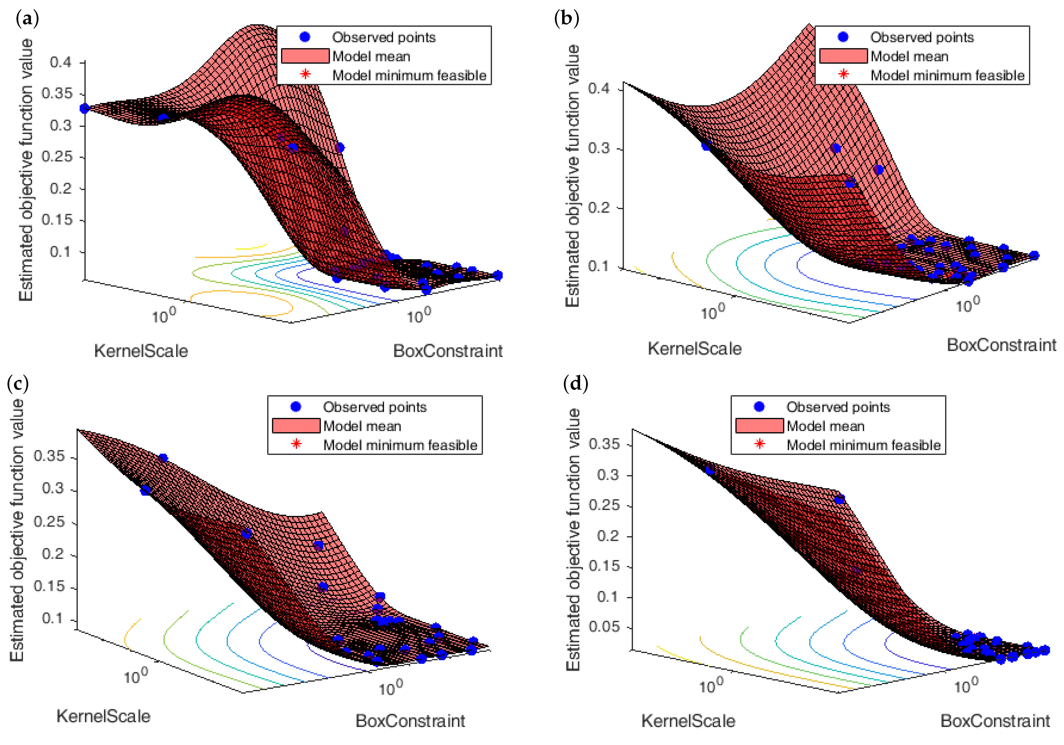
In this study, the SVM was used to predict the trend of the buying behaviour towards life insurance policy from the demographic/economic/psychographic variables. Figure 3 illustrates the Bayesian optimisation routine for estimating the box constraint () and kernel scale () for four different SVM models. Notably, to predict the trend of the buyer/non-buyer on the basis of core factors; the SVM I model, SVM II model and SVM III model were developed which includes the respective statistically significant demographic, economic and psychographic factors as feature space. While the SVM IV model has been proposed by uniting the feature space of all the aforementioned factors.
Observing Figure 3, it can be stated that the minimum feasible objective function value for all SVM models has been found at different combinations of and , i.e., = 975.56 and = 1.0141 for SVM I model, = 7.05 and = 0.0022 for SVM II model, = 284.38 and = 1.5416 for SVM III model, and = 539.37 and = 0.0747 for SVM IV model. The respective combinations of and for each model were used to estimate the performance of the SVM models with the help of five performance metrics specified in Table 7.
From Table 7, it can be stated that the SVM IV model has outperformed in terms of all metrics, and is able to accurately detect the potential consumers with an accuracy of 98.82%. Notably, the area under the curve (AUC) of the SVM IV model is unity, which clearly suggests that the accuracy of the detection of true buyers is extremely accurate. Among the remaining three models, the demographic-based SVM model (i.e., SVM I model) is also able to achieve the desired accuracy. Hence, it can be asserted that the life insurance company can easily target its potential buyers by simply collecting the demographic data of the individuals, and the company still has high chances of accurately detecting the potential buyers. Notably, ideally the value of AUC and Matthew’s correlation coefficient (MCC) is unity.
4.2. Logistic Regression
The logistic model explains the strength of the relationship between the independent and dependent variables. As the relationship is non-linear due to its dichotomous nature (sigmoidal curve), the dependent variable is presented in logit form. Logit is a result of taking the natural logarithm of odds of the dependent variable. Odds can be defined as the ratio of the probability of occurrence of an event with respect to the probability of no-occurrence of an event. The simple logistic equation can be written as follows:
where Y is the dependent dichotomous variable and X is the independent variable (sub-factors) which can be a continuous or categorical variable. is the scalar bias of the Y variable and is the coefficient of regression. The magnitude of the relationship between the independent and dependent variables is described by the value of [68].
In this study, the logistic regression is another supervised machine learning algorithm that is employed to predict the trend of the buying behaviour towards the life insurance policy from the demographic/economic/psychographic variables. In our case, the buying behaviour is a dichotomous variable composed of two categories—namely buyer and non-buyer. Logistic regression is vital for finding the trend of the buyers and non-buyers against a particular demographic/economic/psychographic variable, like how an increase in age is influencing a person to buy a life insurance policy. By investigating this fact, the life insurance companies can easily target a particular cluster of individuals having a specific demographic variable which tends to show a positive trend in the logistic model. The resulting tables of logistic regression are simulated in MATLAB software.
Table 8 shows the logistic regression models predicting the buyer/non-buyer trend based on demographic, economic, psychographic and all combined factors. The logit I model includes only the demographic factors for predicting the buying behaviour, and in a similar fashion logit II and III models include economic and psychographic factors, respectively, for predicting the buying behaviour of a life insurance policy. The fourth model (logit IV) accesses the impact of all three major factors on the prediction of a consumer’s buying behaviour. The coefficient of regression (), scalar bias () and its significance values (p-values) are given to recommend the likelihood of each sub-factor to be included in the respective logit model. If the p-value < 0.05, then the sub-factor is significant in deciding the buying behaviour of life insurance policy.
The first logistic model (logit I model) given in Table 8 with respective values in Table 9, shows that there is a positive relation between five sub-factors (i.e., city, age, education, employment, and number of dependents) and the log odd of the respondent being a buyer of a life insurance policy (p-value < 0.05). The corresponding value of expected for the city is 2.041 (≈), which shows that at a fixed value of other variables, unity increase in a respondent from a larger city (in terms of population size), there is a 2.041-fold increase in a chance that a respondent will buy a life insurance policy. On the other hand, age with a value of ) indicates that the increase in unity in higher age groups yields a 4.38-fold increment in the chances of buying life insurance policy by the respondent. The similar trend can also be observed for education, employment and number of dependents.
Observing the logit II model, it can be asserted that the monthly income and wealth (in the form of land, house, vehicle) plays a significant role in deciding the buying behaviour of a life insurance policy by the respondent. Among all the sub-factors in the logit II model, a vehicle contributes the highest in incrementing the chances of buying a life insurance policy.
On the other hand, the logit III model depicts the impact of psychographic factors on the buying behaviour of a life insurance policy. From Table 8, it can be observed that some sub-factors like savings and risky investment shows negative relation to the log odds of the buyer (p-value < 0.05). These three factors indicate that policy-favouring customers are usually non-regular savers and consider a life insurance policy as a non-risky investment. Similar to all aforementioned logit models, a combined logistic model, i.e., the logit IV model, is also developed, which includes all the elements or sub-factors of demographic, economic and psychographic factors.
The prediction accuracy of all four logit models has been analysed with the help of performance metrics, namely accuracy, area under the curve (AUC), buyers’ and non-buyers’ positive predictive value (PPV), and buyers’ and non-buyers’ false discovery rate (FDR). Notably, higher values of accuracy, AUC, and PPV resemble the better performance of the model in predicting the respondents who are potential buyers. Ideally, the values of accuracy, AUC and PPV should be 100%—while the value of FDR should be 0%. Observing Table 10, it can be asserted that the logit IV model has the highest accuracy (89.2%), AUC (0.95), buyer’s PPV (90%), and lowest buyer’s FDR (10%). However, the psychographic model (logit III model) has the best performance in terms of non-buyers’ PPV and non-buyers’ FDR.
5. Conclusions
Attaining sustainable growth in the life insurance market in India is a need of innovation, which can contribute to accelerating the economic growth of the country. Currently, the life insurance market in India is drifting at a reasonable pace, but it still requires strong measures to sustain the growth of a company and also requires planned consumer penetration effort by the company through tailored life insurance products. The perception of the consumer towards opting for life insurance product depends on various factors which revolve around three core factors, which are demographic, economic and psychographic factors. Focusing on the current situation of the life insurance market in India, it can be asserted that accurately targeting the customers by classifying them through an intelligent decision support system can help the insurance company in sustaining its market share. This study, which was conducted on real-world data collected through a questionnaire, can vastly help in estimating the prospective elements in clustering the behaviour of the consumer towards core life insurance products. Out of the two proposed machine learning-based decision support systems, the SVM-based model can accurately identify the cluster of potential buyers with an overall accuracy of 98.82%, which is much more desirable from the perspective of reliability while targeting potential customers for sustainable growth. The substantial accuracy of the SVM model asserts that intelligent decision making does not require in-depth user-based knowledge of the scenario to reach an optimal solution, and hence can be efficiently used to target potential consumers. In the future, the more complex behavioural features of a consumer from a large number of cities could be collected and studied through a machine learning approach. Furthermore, in order to facilitate the subsequent learning of the intelligent system, it is desirable to develop a map of redundancy relationship among the features.
Supplementary Materials
The following are available online at https://www.mdpi.com/article/10.3390/math9121369/s1, Table S1: Questionnaire, Figure S1: Respondents distributed in terms of buyers and non-buyers for all three cities, Figure S2: Respondents distributed in terms of buyers and non-buyers for gender, Figure S3: Respondents distributed in terms of buyers and non-buyers according to age groups, Figure S4: Respondents distributed in terms of buyers and non-buyers according to marital status, Figure S5: Respondents distributed in terms of buyers and non-buyers according to educational qualification, Figure S6: Respondents distributed in terms of buyers and non-buyers according to employment status, Figure S7: Respondents distributed in terms of buyers and non-buyers according to monthly earning, Figure S8: Respondents distributed in terms of buyers and non-buyers according to monthly saving, Figure S9: Respondents distributed in terms of buyers and non-buyers according to number of dependents, Figure S10: Respondents distributed in terms of buyers and non-buyers according to ownership of farm/land and house/flat, Figure S11: Respondents distributed in terms of buyers and non-buyers according to ownership of four and two wheelers.
Author Contributions
Conceptualisation, M.F.K. and F.H.; methodology, M.F.K. and F.H.; data curation, M.F.K. and F.H.; formal analysis, M.F.K. and F.H.; visualisation, M.F.K. and F.H.; supervision, M.F.K.; funding acquisition, M.M.; writing—original draft preparation and editing, M.F.K. and F.H.; writing—review, M.F.K., F.H., A.A.-H.; project administration, M.F.K. and M.M. All authors have read and agreed to the published version of the manuscript.
Funding
This research received no external funding.
Institutional Review Board Statement
Not applicable.
Informed Consent Statement
Not applicable.
Data Availability Statement
Not applicable.
Conflicts of Interest
The authors declare no conflict of interest.
References
- Nguyen, H.T.; Nguyen, H.; Nguyen, N.D.; Phan, A.C. Determinants of customer satisfaction and loyalty in Vietnamese life-insurance setting. Sustainability 2018, 10, 1151. [Google Scholar] [CrossRef] [Green Version]
- Chang, M.; Jang, H.B.; Li, Y.M.; Kim, D. The relationship between the efficiency, service quality and customer satisfaction for state-owned commercial banks in China. Sustainability 2017, 9, 2163. [Google Scholar] [CrossRef] [Green Version]
- Schiffman, J.B.; Wisenblit, J. Consumer Behavior, 12th ed.; Prentice Hall: New York, NY, USA, 2018. [Google Scholar]
- Solomon, M.R. Consumer Behavior: Buying, Having, and Being, 12th ed.; Prentice Hall: New York, NY, USA, 2016. [Google Scholar]
- Hawkins, D.I.; Mothersbaugh, D.L. Consumer Behavior: Building Marketing Strategy, 11th ed.; McGraw-Hill Irwin: Boston, MA, USA, 2010. [Google Scholar]
- Chen-Yu, H.J.; Kincade, D.H. Effects of product image at three stages of the consumer decision process for apparel products: Alternative evaluation, purchase and post-purchase. J. Fash. Mark. Manag. 2001, 5, 29–43. [Google Scholar]
- Callen, K.S.; Ownbey, S.F. Associations between demographics and perceptions of unethical consumer behaviour. Int. J. Consum. Stud. 2003, 27, 99–110. [Google Scholar] [CrossRef]
- Handbook on Indian Insurance Statistics 2016–2017. Available online: https://irdai.gov.in (accessed on 16 January 2019).
- Ghosh, A. Does life insurance activity promote economic development in India: An empirical analysis. J. Asia Bus. Stud. 2013, 7, 31–43. [Google Scholar] [CrossRef]
- Srivastava, A.; Tripathi, S.; Kumar, A. Indian life insurance industry—The changing trends. Res. World Int. Ref. Soc. Sci. J. 2012, 3, 93–98. [Google Scholar]
- Miklosik, A.; Kuchta, M.; Evans, N.; Zak, S. Towards the adoption of machine learning-based analytical tools in digital marketing. IEEE Access 2019, 7, 85705–85718. [Google Scholar] [CrossRef]
- Abakouy, R.; En-naimi, E.M.; Haddadi, A.E.; Lotfi, E. Data-driven marketing: How machine learning will improve decision-making for marketers. In International Conference Proceeding Series, Proceedings of the Fourth International Conference on Smart City Applications, Casablanca, Morocco, 2–4 October 2019; ACM: New York, NY, USA, 2019; pp. 1–5. [Google Scholar]
- Frederiks, E.R.; Stenner, K.; Hobman, E.V. Household energy use: Applying behavioural economics to understand consumer decision-making and behaviour. Renew. Sustain. Energy Rev. 2015, 41, 1385–1394. [Google Scholar] [CrossRef] [Green Version]
- Armstrong, J.S. Prediction of consumer behavior by experts and novices. J. Consum. Res. 1991, 18, 251–256. [Google Scholar] [CrossRef] [Green Version]
- Haider, F.; Shamsuzzama, M. Mathematical model of policy holder switching within the life insurance market. Int. J. Manag. Sci. Eng. Manag. 2018, 13, 280–285. [Google Scholar] [CrossRef]
- Khodabandehlou, S.; Rahman, M.Z. Comparison of supervised machine learning techniques for customer churn prediction based on analysis of customer behavior. J. Syst. Inf. Technol. 2017, 19, 66–93. [Google Scholar] [CrossRef]
- Noori, A.; Bonakdari, H.; Salimi, A.H.; Gharabaghi, B. A group Multi-Criteria Decision-Making method for water supply choice optimization. Socio-Econ. Plan. Sci. 2021. [Google Scholar] [CrossRef]
- Cassaigne, N.; Singh, M.G. Intelligent decision support for the pricing of products and services in competitive consumer markets. IEEE Trans. Syst. Man Cybern. Part C (Appl. Rev.) 2001, 31, 96–106. [Google Scholar] [CrossRef]
- Xia, Y. Competitive strategies and market segmentation for suppliers with substitutable products. Eur. J. Oper. Res. 2011, 210, 194–203. [Google Scholar] [CrossRef]
- Census Data of India. 2011. Available online: http://censusindia.gov.in/ (accessed on 16 March 2020).
- Rani, P. Factors influencing consumer behaviour. Int. J. Curr. Res. Acad. Rev. 2014, 2, 52–61. [Google Scholar]
- Haider, F.; Shamsuzzama, M. Factors influencing buying behaviour of consumers in life insurance sector: A survey. Organ. Stud. Innov. Rev. 2017, 3, 28–34. [Google Scholar]
- Truett, D.B.; Truett, L.J. The demand for life insurance in Mexico and the United States: A comparative study. J. Risk Insur. 1990, 57, 321–328. [Google Scholar] [CrossRef]
- Sidhardha, D.; Sumanth, M. Consumer buying behavior towards life insurance: An analytical study. Int. J. Commer. Manag. Res. 2017, 3, 1–5. [Google Scholar]
- Liebenberg, A.P.; Carson, J.M.; Hoyt, R.E. The demand for life insurance policy loans. J. Risk Insur. 2010, 77, 651–666. [Google Scholar] [CrossRef]
- Showers, V.E.; Shotick, J.A. The effects of household characteristics on demand for insurance: A Tobit analysis. J. Risk Insur. 1994, 61, 492–502. [Google Scholar] [CrossRef]
- Yusuf, T.O.; Gbadamosi, A.; Hamadu, D. Attitudes of Nigerians towards insurance services: An empirical study. Afr. J. Account. Econ. Financ. Bank. Res. 2009, 4, 34–46. [Google Scholar]
- Chen, R.; Wong, K.A.; Lee, H.C. Age, period, and cohort effects on life insurance purchases in the US. J. Risk Insur. 2001, 68, 303–327. [Google Scholar] [CrossRef] [Green Version]
- Bernheim, B.D. How strong are bequest motives? Evidence based on estimates of the demand for life insurance and annuities. J. Political Econ. 1991, 99, 899–927. [Google Scholar] [CrossRef] [Green Version]
- Gandolfi, A.S.; Laurence, M. Gender-based differences in life insurance ownership. J. Risk Insur. 1996, 63, 683–693. [Google Scholar] [CrossRef]
- Burnett, J.J.; Palmer, B.A. Examining life insurance ownership through demographic and psychographic characteristics. J. Risk Insur. 1984, 51, 453–467. [Google Scholar] [CrossRef]
- Duker, J.M. Expenditure for life insurance among working wife-families. J. Risk Insur. 1969, 36, 525–533. [Google Scholar] [CrossRef]
- Hammond, J.D.; Houston, D.B.; Melander, E.R. Determinants of household life insurance premium expenditures: An empirical investigation. J. Risk Insur. 1967, 34, 397–408. [Google Scholar] [CrossRef]
- Ferber, R.; Lee, L.C. Acquisition and accumulation of life insurance in early married life. J. Risk Insur. 1980, 47, 713–734. [Google Scholar] [CrossRef]
- Kumar, A. Investigating household choice for health and life insurance. Appl. Econ. Lett. 2019, 26, 267–273. [Google Scholar] [CrossRef]
- Xiao, J.J.; Porto, N. Financial education and insurance advice seeking. Geneva Pap. Risk Insur. Issues Pract. 2019, 44, 20–35. [Google Scholar] [CrossRef]
- Tati, R.K.; Baltazar, E.B.B. Factors influencing the choice of investment in life insurance policy. Theor. Econ. Lett. 2018, 8, 3664–3675. [Google Scholar] [CrossRef] [Green Version]
- Uppily, R. A study on consumer behaviour on life insurance products—With reference to private bank employees in Chennai. Int. J. Eng. Manag. Res. 2016, 6, 644–651. [Google Scholar]
- Yazid, A.S.; Arifin, J.; Hussin, M.R.; Daud, W.N.W. Determinants of family takaful (Islamic life insurance) demand: A conceptual framework for a Malaysian study. Int. J. Bus. Manag. 2012, 7, 115–127. [Google Scholar] [CrossRef] [Green Version]
- Curak, M.; Kljakovic-Gaspic, M. Economic and social determinants of life insurance consumption: Evidence from central and eastern Europe. J. Am. Acad. Bus. 2011, 16, 216–222. [Google Scholar]
- Li, D.; Moshirian, F.; Nguyen, P.; Wee, T. The demand for life insurance in OECD countries. J. Risk Insur. 2007, 74, 637–652. [Google Scholar] [CrossRef]
- Hau, A. Liquidity, estate liquidation, charitable motives, and life insurance demand by retired singles. J. Risk Insur. 2000, 67, 123–141. [Google Scholar] [CrossRef] [Green Version]
- Browne, M.J.; Kim, K. An international analysis of life insurance demand. J. Risk Insur. 1993, 60, 616–634. [Google Scholar] [CrossRef]
- Anderson, D.R.; Nevin, J.R. Determinants of young marrieds’ life insurance purchasing behavior: An empirical investigation. J. Risk Insur. 1975, 42, 375–387. [Google Scholar] [CrossRef]
- Black, K.; Skipper, H.D. Life Insurance, 12th ed.; Prentice-Hall: Hoboken, NJ, USA, 1994. [Google Scholar]
- Mantis, G.; Farmer, R.N. Demand for life insurance. J. Risk Insur. 1968, 35, 247–256. [Google Scholar] [CrossRef]
- Baek, E.; DeVaney, S.A. Human capital, bequest motives, risk, and the purchase of life insurance. J. Pers. Financ. 2005, 4, 62–84. [Google Scholar]
- Curak, M.; Dzaja, I.; Pepur, S. The effect of social and demographic factors on life insurance demand in Croatia. Int. J. Bus. Soc. Sci. 2013, 4, 65–72. [Google Scholar]
- Sharma, N. A study of buying behaviour of consumers towards life insurance policies. Glob. J. Res. Bus. Manag. 2018, 6, 477–483. [Google Scholar]
- Meko, M.; Lemie, K.; Worku, A. Determinant of life insurance demand in Ethiopia. J. Econ. Bus. Account. Vent. 2019, 21, 293–302. [Google Scholar] [CrossRef] [Green Version]
- Beenstock, M.; Dickinson, G.; Khajuria, S. The determination of life premiums: An international cross-section analysis 1970–1981. Insur. Math. Econ. 1986, 5, 261–270. [Google Scholar] [CrossRef]
- Stafford, M.R. Marital influence in the decision-making process for services. J. Serv. Mark. 1996, 10, 6–21. [Google Scholar] [CrossRef]
- Redzuan, H.; Rahman, Z.A.; Aidid, S.S.S.H. Economic determinants of family takaful consumption: Evidence from Malaysia. Int. Rev. Bus. Res. Pap. 2009, 5, 193–211. [Google Scholar]
- Outreville, J.F. Life insurance markets in developing countries. J. Risk Insur. 1996, 63, 263–278. [Google Scholar] [CrossRef]
- Campbell, R.A. The demand for life insurance: An application of the economics of uncertainty. J. Financ. 1980, 35, 1155–1172. [Google Scholar] [CrossRef]
- Fortune, P. A theory of optimal life insurance: Development and tests. J. Financ. 1973, 28, 587–600. [Google Scholar]
- Savvides, S. Inquiry into the macroeconomic and household motives to demand life insurance: Review and empirical evidence from Cyprus. J. Bus. Soc. 2006, 19, 37–79. [Google Scholar]
- Beck, T.; Webb, I. Economic, demographic, and institutional determinants of life insurance consumption across countries. World Bank Econ. Rev. 2003, 17, 51–88. [Google Scholar] [CrossRef] [Green Version]
- Sen, S. An Analysis of Life Insurance Demand Determinants for Selected Asian Economies and India; Madras School of Economics: Chennai, India, 2008. [Google Scholar]
- Headen, R.S.; Lee, J.F. Life insurance demand and household portfolio behavior. J. Risk Insur. 1974, 41, 685–698. [Google Scholar] [CrossRef]
- Karni, E.; Zilcha, I. Uncertain lifetime, risk aversion and life insurance. Scand. Actuar. J. 1985, 2, 109–123. [Google Scholar] [CrossRef]
- Nam, Y.; Hanna, S.D. The effects of risk aversion on life insurance ownership of single-parent households. Appl. Econ. Lett. 2019, 26, 1285–1288. [Google Scholar] [CrossRef]
- Zelizer, V.A.R. Morals and Markets: The Development of Life Insurance in the United States, Legacy ed.; Columbia University Press: New York, NY, USA, 2017. [Google Scholar]
- Hofflander, A.E.; Duvall, R.M. Inflation and sales of life insurance. J. Risk Insur. 1967, 34, 355–361. [Google Scholar] [CrossRef]
- Noble, W.S. What is a support vector machine? Nat. Biotechnol. 2006, 24, 1565–1567. [Google Scholar] [CrossRef] [PubMed]
- Pregibon, D. Logistic regression diagnostics. Ann. Stat. 1981, 9, 705–724. [Google Scholar] [CrossRef]
- Lee, Y.J.; Mangasarian, O.L. SSVM: A smooth support vector machine for classification. Comput. Optim. Appl. 2001, 20, 5–22. [Google Scholar] [CrossRef]
- Peng, C.Y.J.; Lee, K.L.; Ingersoll, G.M. An introduction to logistic regression analysis and reporting. J. Educ. Res. 2002, 96, 3–14. [Google Scholar] [CrossRef]
Figure 1.
Heat map of 937 responses obtained from three major cities in India.

Figure 2.
Box plot of 937 responses obtained from three major cities in India.

Figure 3.
Estimation of box constraint () and kernel scale () of SVM models using Bayesian optimisation by choosing a different feature set which is comprised of (a) demographic factors; (b) economic factors; (c) psychographic factors; and (d) all factors combined together.
Figure 3.
Estimation of box constraint () and kernel scale () of SVM models using Bayesian optimisation by choosing a different feature set which is comprised of (a) demographic factors; (b) economic factors; (c) psychographic factors; and (d) all factors combined together.


Table 1.
Results of test between demographic factors and buying behaviour of buyers/non-buyers of a life insurance policy.
Table 1.
Results of test between demographic factors and buying behaviour of buyers/non-buyers of a life insurance policy.
| Demographics | Value | df | p-Value | Null Hypothesis (Rejected/Accepted) | Association |
|---|---|---|---|---|---|
| City | 9.026 | 2 | 0.011 | Reject | Yes |
| Gender | 0.650 | 1 | 0.420 | Accept | No |
| Age | 178.764 | 4 | 1.374 | Reject | Yes |
| Marital status | 132.487 | 2 | 1.701 | Reject | Yes |
| Education | 87.626 | 4 | 4.203 | Reject | Yes |
| Employment | 210.507 | 4 | 2.067 | Reject | Yes |
| No. of dependents | 32.165 | 4 | 2.000 | Reject | Yes |
Table 2.
Goodman and Kruskal’s gamma correlation between demographic factors and buyer/non-buyer.
| Demographics | Gamma () Value | p-Value | Null Hypothesis (Rejected/Accepted) | Association |
|---|---|---|---|---|
| City | −0.129 | 0.020 | Reject | Yes |
| Gender | −0.058 | 0.418 | Accept | No |
| Age | −0.620 | 3.004 | Reject | Yes |
| Marital status | 0.322 | 6.148 | Reject | Yes |
| Education | −0.496 | 2.029 | Reject | Yes |
| Employment | −0.135 | 0.018 | Reject | Yes |
| No. of dependents | −0.266 | 9.236 | Reject | Yes |
Table 3.
Results of test on economic factors and buying behaviour of buyers and non-buyers of a life insurance policy.
Table 3.
Results of test on economic factors and buying behaviour of buyers and non-buyers of a life insurance policy.
| Economic Factors | Value | df | p-Value | Null Hypothesis (Rejected/Accepted) | Association |
|---|---|---|---|---|---|
| Monthly income | 250.362 | 4 | 5.440 | Reject | Yes |
| Monthly saving | 136.753 | 4 | 1.380 | Reject | Yes |
| Farm/land | 67.679 | 4 | 7.012 | Reject | Yes |
| House/Flat | 124.915 | 3 | 6.739 | Reject | Yes |
| Four wheeler | 147.721 | 2 | 8.372 | Reject | Yes |
| Two wheeler | 29.355 | 2 | 4.223 | Reject | Yes |
Table 4.
Goodman and Kruskal’s gamma correlation between economic factors of buyer/non-buyer.
| Economic Factors | Gamma Value | p-Value | Null Hypothesis (Rejected/Accepted) | Association |
|---|---|---|---|---|
| Monthly income | −0.678 | 6.645 | Reject | Yes |
| Monthly saving | −0.500 | 1.731 | Reject | Yes |
| Farm/land | −0.502 | 2.963 | Reject | Yes |
| House/Flat | −0.580 | 1.521 | Reject | Yes |
| Four wheeler | −0.702 | 7.945 | Reject | Yes |
| Two wheeler | −0.499 | 2.137 | Reject | Yes |
Table 5.
Mean ranks of buyers and non-buyers against psychographic factors.
| Psychographic Factors | Buyer/Non-Buyer | N | Mean Rank |
|---|---|---|---|
| Buyer | 629 | 458.69 | |
| Spend time with family | Non-buyer | 308 | 490.06 |
| Total | 937 | ||
| Buyer | 629 | 381.42 | |
| Very informative | Non-buyer | 308 | 647.85 |
| Total | 937 | ||
| Buyer | 629 | 456.82 | |
| Saving regularly for future | Non-buyer | 308 | 493.88 |
| Total | 937 | ||
| Buyer | 629 | 505.83 | |
| Very particular about religious values | Non-buyer | 308 | 393.78 |
| Total | 937 | ||
| Buyer | 629 | 446.08 | |
| Take my own decision | Non-buyer | 308 | 515.80 |
| Total | 937 | ||
| Buyer | 629 | 462.21 | |
| Inflation is serious issue | Non-buyer | 308 | 482.87 |
| Total | 937 | ||
| Buyer | 629 | 442.18 | |
| Avoid risky investment | Non-buyer | 308 | 523.77 |
| Total | 937 |
Table 6.
Kruskal–Wallis one-way ANOVA between psychographic factors and buying behaviour.
| Spend Time with Family | Very Informative | Saving Regularly for Future | Very Particular about Religious Values | Take My Own Decision | Inflation Is Serious Issue | Avoid Risky Investment | |
|---|---|---|---|---|---|---|---|
| Chi-square | 3.693 | 283.253 | 4.646 | 41.502 | 17.151 | 1.508 | 23.010 |
| df | 1 | 1 | 1 | 1 | 1 | 1 | 1 |
| Asymp. Sig. | 0.055 | 1.140 | 0.031 | 1.177 | 3.500 | 0.219 | 2.000 |
| Null hypothesis | Accept | Reject | Reject | Reject | Reject | Accept | Reject |
Table 7.
Performance analysis of SVM-based decision support models.
| Performance Metrics | SVM I Model | SVM II Model | SVM III Model | SVM IV Model |
|---|---|---|---|---|
| Accuracy (%) | 94.45 | 89.75 | 91.24 | 98.82 |
| AUC | 0.96 | 0.88 | 0.91 | 1.00 |
| Sensitivity (%) | 94.04 | 91.31 | 90.88 | 98.28 |
| Specificity (%) | 95.39 | 86.30 | 92.16 | 100.00 |
| MCC | 0.87 | 0.76 | 0.79 | 0.97 |
Table 8.
Logistic regression models of respondents’ buying behaviour on demographic, economic and psychographic factors.
Table 8.
Logistic regression models of respondents’ buying behaviour on demographic, economic and psychographic factors.
| Factors | Sub-Factors | Logit I Model | Logit II Model | Logit III Model | Logit IV Model | ||||
|---|---|---|---|---|---|---|---|---|---|
| p-Value | p-Value | p-Value | p-Value | ||||||
| City | 0.310 | <0.05 | - | - | - | - | 0.124 | ≥0.05 | |
| Gender | 0.306 | ≥0.05 | - | - | - | - | 1.068 | <0.05 | |
| Age | 0.642 | <0.05 | - | - | - | - | 1.197 | ≥0.05 | |
| Demographic | Marital status | −0.049 | ≥0.05 | - | - | - | - | −0.244 | ≥0.05 |
| Education | 0.633 | <0.05 | - | - | - | - | 0.676 | <0.05 | |
| Employment | 0.239 | <0.05 | - | - | - | - | 0.156 | ≥0.05 | |
| No. of dependents | 0.597 | <0.05 | - | - | - | - | 0.409 | <0.05 | |
| Monthly income | - | - | 0.371 | <0.05 | - | - | 0.123 | ≥0.05 | |
| Monthly saving | - | - | 0.020 | ≥0.05 | - | - | −0.078 | ≥0.05 | |
| Economic | Farm/land | - | - | 0.314 | <0.05 | - | - | −0.173 | ≥0.05 |
| House/flat | - | - | 0.723 | <0.05 | - | - | 0.385 | ≥0.05 | |
| Four wheeler | - | - | 1.151 | <0.05 | - | - | 0.651 | <0.05 | |
| Two wheeler | - | - | 1.269 | <0.05 | - | - | 0.643 | ≥0.05 | |
| Spend time with family | - | - | - | - | −0.258 | ≥0.05 | −0.355 | ≥0.05 | |
| Very informative | - | - | - | - | 2.603 | <0.05 | 3.100 | <0.05 | |
| Saving regularly | - | - | - | - | −0.289 | <0.05 | −0.926 | <0.05 | |
| Psychographic | Religious values | - | - | - | - | 1.053 | <0.05 | 2.154 | <0.05 |
| Take own decision | - | - | - | - | −0.076 | ≥0.05 | 0.333 | ≥0.05 | |
| Inflation is serious issue | - | - | - | - | 0.286 | ≥0.05 | 0.656 | <0.05 | |
| Avoid risky investment | - | - | - | - | −0.554 | <0.05 | −0.468 | <0.05 | |
Table 9.
Respective values of logistic regression models.
| Logit I Model | Logit II Model | Logit III Model | Logit IV Model | ||||
|---|---|---|---|---|---|---|---|
| p-Value | p-Value | p-Value | p-Value | ||||
| −7.054 | <0.05 | −5.002 | <0.05 | 6.005 | <0.05 | −6.545 | <0.05 |
Table 10.
Performance analysis of all logit models.
| Performance Metrics | Logit I Model | Logit II Model | Logit III Model | Logit IV Model |
|---|---|---|---|---|
| Accuracy (%) | 75.9 | 75.7 | 87.0 | 89.2 |
| AUC | 0.84 | 0.80 | 0.83 | 0.95 |
| Buyer’s PPV (%) | 83 | 79 | 85 | 90 |
| Non-buyer’s PPV (%) | 63 | 67 | 94 | 88 |
| Buyer’s FDR (%) | 17 | 21 | 15 | 10 |
| Non-buyer’s FDR (%) | 37 | 33 | 6 | 12 |
Publisher’s Note: MDPI stays neutral with regard to jurisdictional claims in published maps and institutional affiliations. |
© 2021 by the authors. Licensee MDPI, Basel, Switzerland. This article is an open access article distributed under the terms and conditions of the Creative Commons Attribution (CC BY) license (https://creativecommons.org/licenses/by/4.0/).
Share and Cite
MDPI and ACS Style
Khan, M.F.; Haider, F.; Al-Hmouz, A.; Mursaleen, M. Development of an Intelligent Decision Support System for Attaining Sustainable Growth within a Life Insurance Company. Mathematics 2021, 9, 1369. https://doi.org/10.3390/math9121369
AMA Style
Khan MF, Haider F, Al-Hmouz A, Mursaleen M. Development of an Intelligent Decision Support System for Attaining Sustainable Growth within a Life Insurance Company. Mathematics. 2021; 9(12):1369. https://doi.org/10.3390/math9121369
Chicago/Turabian StyleKhan, Mohammad Farhan, Farnaz Haider, Ahmed Al-Hmouz, and Mohammad Mursaleen. 2021. "Development of an Intelligent Decision Support System for Attaining Sustainable Growth within a Life Insurance Company" Mathematics 9, no. 12: 1369. https://doi.org/10.3390/math9121369
Note that from the first issue of 2016, this journal uses article numbers instead of page numbers. See further details here.