On State Occupancies, First Passage Times and Duration in Non-Homogeneous Semi-Markov Chains

Abstract

Semi-Markov processes generalize the Markov chains framework by utilizing abstract sojourn time distributions. They are widely known for offering enhanced accuracy in modeling stochastic phenomena. The aim of this paper is to provide closed analytic forms for three types of probabilities which describe attributes of considerable research interest in semi-Markov modeling: (a) the number of transitions to a state through time (Occupancy), (b) the number of transitions or the amount of time required to observe the first passage to a state (First passage time) and (c) the number of transitions or the amount of time required after a state is entered before the first real transition is made to another state (Duration). The non-homogeneous in time recursive relations of the above probabilities are developed and a description of the corresponding geometric transforms is produced. By applying appropriate properties, the closed analytic forms of the above probabilities are provided. Finally, data from human DNA sequences are used to illustrate the theoretical results of the paper.

1. Introduction

Human populations can be divided into categories (states and classes) taking into account some of their basic characteristics, such as place of residence, social class or rank in a hierarchy system. People usually move from a category to another category in a probabilistic manner and a person’s history contains a sequence of sojourn times in the various categories and a set of transitions that have taken place. These are the basic parameters that construct a semi-Markov chain (SMC), according to which a mathematical model can be developed for the study of those systems [1,2]. These systems do not necessarily have to include humans, instead, they can describe any potential system characterized by and composed of historical observations, such as stay times in situations as well as transitions from one category to another. If, for the study of a population system, we reside on a Markov chain, we assume that the probability of transition from one category in another does not depend on the length of stay. Nonetheless, this time dependence is, in some cases, desirable to include in the process since it provides additional useful information. In this case, the transitions of such a system are not merely described by a typical Markov chain procedure and Semi-Markov models are introduced as the stochastic tools that provide a more rigorous framework accommodating a greater variety of applied probability models [3,4,5]. Various applications of semi-Markov processes include manpower planning, credit risk, word sequencing and DNA analysis [6,7,8,9,10,11,12,13,14].

In addition to semi-Markov processes, the non-homogeneous semi-Markov system (NHSMS) was defined, introducing a class of broader stochastic models [15,16] that provide a more general framework to describe the complex semantics of the system involved. Semi-Markov systems, which deploy a number of Markov chains evolving in parallel, are mostly applied in manpower planning, where the most important issues pertain to the evolution, control and asymptotic behavior [17,18,19]. In the last two decades, there has been an extended body of literature regarding the theory and results about NHMS [20,21,22,23,24,25,26,27,28,29]. The dynamic characteristics of the semi-Markov systems influence the number of times the chain occupies a state, of how long it takes to leave a state as well as the probability of first passage to a state. Therefore, in order to accompany the basic parameters of the semi-Markov chain and to enhance the modeling framework, additional attributes of critical interest are the occupancy, first passage time and duration probabilities, which are described as follows

• Occupancy probabilities. These probabilities describe the distribution of the random variables that define the number of times the SMC has visited a specific state during an arbitrary time interval.
• First passage time probabilities. These are the probabilities that describe the transition from a state to a different state for the first time. The properties of the first passage time probabilities have been investigated for Markov processes and some specific types of semi-Markov processes [30,31,32,33,34,35]. Details for the first passage time probabilities have been also presented for various stochastic processes [36].
• Duration probabilities. These probabilities describe the distribution of random variables that define the time needed for the SMC to transfer to a different state.

DNA sequences are usually studied using probabilistic models, as nucleotide appearances are inter-correlated and attempts to use Markov models to model them have been reported [10,37]. One of the earliest studies applied a Markov model on the nucleotide alphabet $\{A,C,G,T\}$ to estimate the transition probability matrix and the number of doublets and triplets [38]. Several statistics have been proposed to test the dependency order of the sequence, e.g., the Markov order, such as the phi-divergent statistics and conditional mutual information [39,40,41]. More advances in the subject include hidden-Markov models that are able to model different regions of DNA sequences [42]. Word occurrences are also of interest in DNA analysis [43]. Previous studies have examined the distribution, moments and properties of successive word occurrences [44,45]. Papadopoulou has provided some examples of semi-Markov models on modeling biological sequences [46]. Furthermore, algorithmic applications for estimating the first passage time probabilities in genomic sequences have been reported [47].

The aim of this study is to provide insight on the actual mechanism of the recursive relations of the probabilities mentioned above. Section 2 presents the basic parameters of a SMC, the interval transition probabilities and the entrance probabilities. Section 3 presents the main results of the paper, that is, the closed analytic solutions for the occupancy, duration and first passage time probabilities. The final section applies these theoretical results to human genome DNA strands. For the first illustration, the aim is to find the corresponding probabilities between nucleotide words and their symmetric complements by using the analytic form of the first passage time probabilities. Finally, for the second illustration, the frequency of the dinucleotide $GC$ is examined for two distinct DNA sequences, using the occupancy probabilities.

2. Basic Framework

We can consider the semi-Markov chain ${\left\{X_t\right\}}_{t\ge 1}$ with state space $S=\{1,2,\dots ,N\}$ as a discrete stochastic process in which the successive states are defined by the transition probability matrix and the sojourn time in each state is described by a random variable conditioned on the current and the next state to be transitioned into. Thus, during the transition times, the process is equivalent to a Markov process. We call this Markovian process the embedded process. Let transition probabilities $p_{ij}\left(t\right)$ be the probability of a SMC provided that it entered state i during its last transition at time t to transition to state j in the next transition. The transition probabilities should satisfy the same equations of a Markovian process, that is, $p_{ij}\ge 0,\forall i,j\in S$ and ${\sum }_{j=1}^N{p}_{ij}=1,\forall i\in S$. When the process enters state i at time t, we assume that this state determines the next transition to state j, which occurs according to the transition probabilities. However, before making the transition from state i to state j and after the next state j is selected, the chain holds in state i for time ${\tau }_{ij}$. The sojourn time ${\tau }_{ij}$ is a positive random variable with density function $h_{ij}(·)$, which is called the function of sojourn time to transition from state i to state j. Thus, $Prob[{\tau }_{ij}=m]=h_{ij}\left(m\right)$, for $m=1,2,..,$ and $i,j\in S$. We assume that the mean values of the distributions of sojourn times are finite and $h_{ij}\left(0\right)=0.$ In matrix notation, the basic parameters of the semi-Markov chain are the sequence of transition matrices ${\left\{\mathit{P}\left(t\right)\right\}}_{t=0}^{\infty }$ and the sequence of sojourn time matrices ${\left\{\mathit{H}\left(m\right)\right\}}_{m=1}^{\infty }$. The probabilities of the waiting times $w_i(t,m)$ are defined as follows:

$$w_i(t,m)=\sum _{j=1}^N{p}_{ij}\left(t\right)h_{ij}\left(m\right)=Prob[{\tau }_i=m|t],$$

where ${\tau }_i$ is the holding time of the SMC in state i. The core matrix of the SMC connects the transition probabilities and the sojourn times and it is defined as follows:

$$\mathit{C}(t,m)={\left\{c_{ij}(t,m)\right\}}_{ij\in S}=\mathit{P}\left(t\right)\circ \mathit{H}\left(m\right).$$

The operator $\{\circ \}$ denotes the element-wise product of matrices (Hadamard product). Using the core matrix, we define $q_{ij}\left(k\right|t,n)$, which is the joint probability that the SMC will be in state j at time $t+n$ and that it has made k transitions during the time interval $(t,t+n]$, given that at time t the process has entered state i. In order to calculate the probability $q_{i,j}\left(k\right|t,n)$, we distinguish two cases. First, we consider that during the time interval $(t,t+n]$ the number of transitions is zero. Then, in order for the process at time $t+n$ to be in state j, given that no transitions were made, it must be that the states $i,j$ are the same. Secondly, assume that the SMC makes the first transition to state r at time $t+m,0<m<n$. Then, in the time interval $(t,t+m]$, we have one transition to state r and, in the remaining time interval $(t+m,t+n]$, we have the remaining $k-1$ transitions, with a final transition to state j. Thus, the resulting formula is as follows:

$$q_{ij}\left(k\right|t,n)={\delta }_{ij}\delta {\left(k\right)}^{>}{w}_i(t,n)+\sum _{r=1}^N\sum _{m=0}^n{c}_{ir}(t,m)q_{rj}(k-1|t+m,n-m).$$

where ${}^{>}{w}_i(t,n)={\sum }_{k=n+1}^{\infty }{w}_i(t,k)$ indicates the survival function of $w_i(t,n)$ and $\delta \left(k\right)=1$ if k is zero, otherwise it is zero. If we are not interested in counting the number of transitions up to the final state j, we can deduce the following recursive relationship.

$$q_{ij}(t,n)={\delta }_{ij}^{>}{w}_i(t,n)+\sum _{r=1}^N\sum _{m=0}^n{c}_{ir}(t,m)q_{rj}(t+m,n-m).$$

We also define the quantity $e_{i,j}\left(k\right|t,n)$, which is the probability that the SMC enters state j at time $t+n$ and the total number of transitions in the time interval $(t,t+n]$ is k, given that the SMC has entered state i at the initial position. Here, we can distinguish two cases. First, we assume that the number of transitions in the time interval $(t,t+n]$ is zero. Then, to enter in state j at time $t+n$, the states i and j must be the same since state i was entered at the initial time. For the second case, suppose that the SMC at time $t+m,0<m<n$ makes its first transition to state r. Then, at the time interval $(t,t+m]$ we have a transition to state r and, at the time interval $(t+m,t+n]$, we have the remaining $k-1$ transitions, with the final transition to state j. These facts result in the following recursive relationship.

$$e_{ij}\left(k\right|t,n)={\delta }_{ij}\delta \left(n\right)\delta \left(k\right)+\sum _{r=1}^N\sum _{m=0}^n{c}_{ir}(t,m)e_{rj}(k-1|t+m,n-m).$$

If we are not interested in the number of transitions up to the final state j, we can reduce the recursive relationship to the quantity $e_{ij}(t,n)$, which are the probabilities that the SMC will enter state j at time n, provided that, at the initial position at time t, the SMC has entered state i. The equation for calculating the probabilities $e_{ij}(t,n)$ is given by the following.

$$e_{ij}(t,n)={\delta }_{ij}\delta \left(n\right)+\sum _{r=1}^N\sum _{m=0}^n{c}_{ir}(t,m)e_{rj}(t+m,n-m).$$

The interval transition probabilities and entrance probabilities are connected by the following relationship.

$$q_{ij}\left(k\right|t,n)=\sum _{m=0}^n{e}_{ij}{\left(k\right|t,m)}^{>}{w}_j(t+m,n-m).$$

3. Theoretical Results: Analytic Solutions of the Recursive Equations

3.1. First Passage Time

The first passage times provide a measure of how long it takes to reach a given state from another. We can think of first passage times either in terms of transitions or of time or both. Thus, let $f_{ij}\left(k\right|t,n)$ be the probability that k transitions and time n will be required for the first passage from state i to state j given that the SMC entered state i at time t. Applying a probabilistic argument, we can provide the following recursive formula.

$$f_{ij}\left(k\right|t,n)=\sum _{r\ne j}^N\sum _{m=0}^n{c}_{ir}(t,m)f_{rj}(k-1|t+m,n-m)+\delta (k-1)c_{ij}(t,n).$$

(1)

The first term of Equation $\left(1\right)$ corresponds to the case where $k>1$ and the SMC makes a transition to some state r different from j at time $t+m$ and then makes a first passage from r to j in $k-1$ transitions during the interval $(t+m,n-m]$. The term is summed over all states and holding times that could describe the first transition. The second term corresponds to the case where $k=1$ and the process moves directly to state j at time $t+n$. If we are not interested in counting the transitions, then the recursive formula of the probabilities $f_{ij}(t,n)$ is provided by the following.

$$f_{ij}(t,n)=\sum _{r\ne j}^N\sum _{m=0}^n{c}_{ir}(t,m)f_{rj}(t+m,n-m)+c_{ij}(t,n).$$

(2)

Theorem 1.

For each non-homogeneous SMC with discrete state space $S=1,2,\dots ,N$, a sequence of transition probability matrices ${\left\{\mathit{P}\left(t\right)\right\}}_{t=0}^{\infty }$ and a sequence of sojourn time matrices ${\left\{\mathit{H}\left(m\right)\right\}}_{m=1}^{\infty }$, the probability matrices of first passage times $\mathbf{F}\left(k\right|t,n)={\left\{f_{ij}\left(k\right|t,n)\right\}}_{i,j\in S}$ are given by the following relationships:

• $\mathbf{F}\left(1\right|t,n)=\mathbf{C}(t,n),$ for every n.
• $\mathbf{F}\left(k\right|t,n)=\mathbf{0},$ if $k>n$ or $k=0$.
• $\mathbf{F}\left(k\right|t,n)={\sum }_{m_1=1}^{n-k+1}\ast {\sum }_{m_2=1+m_1}^{n-k+2}\ast \dots \ast {\sum }_{m_{k-1}=1+m_{k-2}}^{n-1}{{\prod }_{r=0}^{k-1}}^{\left\{\mathbf{B}\right\}}\mathbf{C}\left(t+m_{k-r-1},m_{k-r}-m_{k-r-1}\right),\mathit{for}\mathit{each}1<k\le n$,

where $\mathbf{B}=\mathbf{U}-\mathbf{I}$, $\mathbf{U}={\{u_{ij}=1\}}_{i,j\in S}$, $\mathbf{I}$ is the $N\times N$ identity matrix and

$$\begin{array}{cc}\hfill & \prod _{r=0}^{k-1}{}^{\left\{\mathbf{B}\right\}}\mathbf{C}\left(s+m_{k-r-1},m_{k-r}-m_{k-r-1}\right)=\hfill \\ \hfill & =\left.\mathbf{C}\left(s,m_1\right)\left\{\mathbf{C}\left(s+m_1,m_2-m_1\right)\left\{\dots \left\{\mathbf{C}\left(s+m_{k-1},n-m_{k-1}\right)\circ \mathbf{B}\right\}\circ \mathbf{B}\right\}\dots \right\}\circ \mathbf{B}\right\}.\hfill \end{array}$$

Proof. 

Appendix A.1. □

3.2. Duration

Transitions of a SMC can be divided into two categories: virtual and real. The first category refers to transitions made from one state to the same state, while the second category refers to transitions from one state to a different state. Based on those two categories, one can define the duration as the number of transitions or the time required for the SMC to leave the initial state and to move to a different state, i.e., a real transition to take place for the first time and not a virtual one. Therefore, it is of interest to study the duration probability $d_i\left(k\right|t,n)$ defined as the probability that the SMC moves for the first time to a different state that the initial one after n time units and k transitions during the interval $(t,t+n]$, given that the process entered state i at time t. We note here that out of the total k transitions in the above case, $k-1$ transitions are virtual and one transition is real. The duration probabilities for $k\le n$ are provided by the following.

$$d_i\left(k\right|t,n)=\sum _{m=0}^n{c}_{ii}(t,m)d_i(k-1|t+m,n-m)+\delta (k-1)\left({\mathrm{w}}_i(t,n)-c_{ii}(t,n)\right).$$

(3)

In the case that $k>n$ or $k=0$, then $d_i\left(k\right|t,n)=0$. The rationale of this relationship can be deconstructed into two parts. In the first part, we can assume that the SMC has at least one virtual intermediate transition, while it starts from state i at time t, holds at the state i for m time units and finally transfers to state i again. At this point, the associated probability is $d_i(k-1|t+m,n-m)$. In the second scenario, we assume that the SMC makes no transition up to time $t+n$. Therefore, the chain holds at state i for exactly n time units and then moves to a state j different than i. Thus, the duration defined in the present measures how long it takes to leave a given state.

Theorem 2.

For each non-homogeneous SMC with discrete state space $S=1,2,\dots ,N$, a sequence of transition probability matrices ${\left\{\mathit{P}\left(t\right)\right\}}_{t=0}^{\infty }$ and a sequence of sojourn time matrices ${\left\{\mathit{H}\left(m\right)\right\}}_{m=1}^{\infty }$, the duration probability matrices $\mathbf{D}\left(k\right|t,n)=diag{\left\{d_i\left(k\right|t,n)\right\}}_{i\in S}$ are provided by the following relationships:

• $\mathbf{D}\left(1\right|t,n)=\left[\mathbf{W}(t,n)-\mathbf{C}(t,n)\circ \mathbf{I}\right],$ for every n.
• $\mathbf{D}\left(k\right|t,n)=\mathbf{0},$ if $k>n$ or $k=0$.
• $\mathbf{D}\left(k\right|t,n)={\sum }_{m_1=1}^{n-k+1}\ast {\sum }_{m_2=1+m_1}^{n-k+2}\ast \dots \ast {\sum }_{m_{k-1}=1+m_{k-2}}^{n-1}\left(\mathbf{C}\left(t,m_1\right)\circ \mathbf{I}\right)\left(\mathbf{C}\left(t+m_1,m_2-m_1\right)\circ \mathbf{I}\right)\dots$$\left(\mathbf{C}\left(t+m_{k-2},m_{k-1}-m_{k-2}\right)\circ \mathbf{I}\right)\left(\mathbf{W}\left(t+m_{k-1},n-m_{k-1}\right)-\mathbf{C}\left(t+m_{k-1},n-m_{k-1}\right)\circ \mathbf{I}\right),\mathit{for}\mathit{each}1<k\le n$,

where $\mathbf{W}(t,n)=diag{\left\{w_i(t,n)\right\}}_{i\in S}$.

Proof. 

Appendix A.2. □

3.3. Occupancy

We define $v_{ij}(t,n)$ to be the number of times the SMC makes transitions to a state j in time interval of length equal to n, provided that in the initial time t the SMC had entered state i. If the initial state is the same as j, that is when $i=j$, then the initial state is not counted in $v_{ij}(t,n)$. We call the quantity $v_{ij}(t,n)$ as the occupancy measure of state j at time $t+n$, provided that the SMC entered state i at time t. Clearly, the quantity $v_{ij}(t,n)$ is a discrete random variable. We define as ${\omega }_{ij}(·|t,n)$ the probability mass distribution of $v_{ij}(t,n)$, which is ${\omega }_{ij}\left(x\right|t,n)=Prob[v_{ij}(t,n)=x]$. The recursive relationship of the occupancy probabilities is given by the following:

$$\begin{array}{cc}\hfill {\omega }_{ij}\left(x\right|t,n)& =\sum _{\genfrac{}{}{0pt}{}{r=1}{r\ne j}}^N\sum _{m=0}^n{c}_{ir}(t,m){\omega }_{rj}\left(x\right|t+m,n-m)+\hfill \\ \hfill & +\sum _{m=0}^n{c}_{ij}(t,m){\omega }_{jj}(x-1|t+m,n-m)+\delta \left(x\right)>w_i(t,n),\hfill \end{array}$$

(4)

where $i,j\in S,n=0,1,\dots ,\mathrm{and}x=0,1,\dots$.

Assumption 1.

In what follows, we assume that the embedded Markov chain is homogeneous, i.e.,${\left\{\mathit{P}\left(t\right)\right\}}_{t=0}^{\infty }=\mathit{P},$for each t.

Considering the above assumption, one can use the double geometric transform of the occupancy probabilities as follows.

$${\omega }_{ij}^{gg}\left(y\right|z)=\sum _{x=0}^{\infty }\sum _{n=0}^{\infty }{\omega }_{ij}\left(x\right|n)z^n{y}^x.$$

Moreover, from the Equation (4), we can write the double geometric transform of the occupancy probabilities as follows.

$${\omega }_{ij}^{gg}\left(y\right|z)=\sum _{r=1}^N{c}_{ir}^g\left(z\right){\omega }_{rj}^{gg}\left(y\right|z)-(1-y)c_{ij}^g\left(z\right){\omega }_{jj}^{gg}\left(y\right|z){+}^{>}{w}_i^g\left(z\right).$$

In matrix notation, we can use the previous results to obtain the following [3]:

$${\mathsf{\Omega }}^{gg}\left(y\right|z)=\frac{1}{1-z}\mathbf{U}-\frac{1-y}{1-z}{\left[\mathbf{I}-{\mathbf{C}}^g\left(z\right)\right]}^{-1}{\mathbf{C}}^g\left(z\right){\left(y\mathbf{I}+(1-y){\left[\mathbf{I}-{\mathbf{C}}^g\left(z\right)\right]}^{-1}\circ \mathbf{I}\right)}^{-1},$$

where $\mathbf{U}$ is the unit matrix, ${\mathsf{\Omega }}^{gg}\left(y\right|z)={\left\{{\omega }_{ij}^{gg}\left(y\right|z)\right\}}_{i,j\in S}$ is the double geometric transform of $\mathsf{\Omega }\left(x\right|n)={\left\{{\omega }_{ij}\left(x\right|n)\right\}}_{i,j\in S}$ and ${\mathbf{C}}^g\left(z\right)={\left\{c_{ij}^g\left(z\right)\right\}}_{i,j\in S}$.

The occupancy probabilities are connected with the corresponding homogeneous first passage time probabilities through the following relationship.

$${\omega }_{ij}\left(x\right|n)=\delta {\left(x\right)}^{>}{f}_{ij}\left(n\right)+\sum _{m=0}^n{f}_{ij}\left(m\right){\omega }_{jj}(x-1|n-m).$$

Using the double geometric transform, we can present the occupancy probabilities in matrix form according to the geometric transforms of the first passage time probabilities:

$${\mathsf{\Omega }}^{gg}\left(y\right|z)={}^{>}{\mathbf{F}}^g\left(z\right)+y{\mathbf{F}}^g\left(z\right)\left[{}^{>}{\mathbf{F}}^g\left(z\right)\circ \mathbf{I}\right]{\left[\mathbf{I}-y\left({\mathbf{F}}^g\left(z\right)\circ \mathbf{I}\right)\right]}^{-1},$$

which could be further simplified by using ${}^{>}{f}_{ij}^g\left(z\right)=\frac{1-f_{ij}^g\left(z\right)}{1-z}$ (Appendix B.1) resulting in matrix notation in (Appendix B.2).

$${\mathsf{\Omega }}^{gg}\left(y\right|z)=\frac{1}{1-z}\mathbf{U}-\frac{1-y}{1-z}{\mathbf{F}}^g\left(z\right){\left[\mathbf{I}-y{\mathbf{F}}^g\left(z\right)\circ \mathbf{I}\right]}^{-1}.$$

We now provide Theorem 3 and Lemma 1 that will be used to prove the main Theorem 4 of the occupancy probabilities with respect to the core matrix.

Theorem 3.

For a SMC with core matrix $\mathbf{C}(·)$, we have the following:

$$\begin{array}{c}{\mathsf{\Omega }}^g\left(z\right|n)=(z-1)\sum _{j=1}^{n-1}\left[\mathbf{C}\left(j\right)+\left[\sum _{i=2}^j\left(\mathbf{C}(i-1)+\sum _{k=1}^{i-2}{\mathbf{S}}_i\left(k,m_k\right)\right)\mathbf{C}(j+1-i)\right]\left[{\mathsf{\Omega }}^g\left(z\right|n-j)\right]\circ \mathbf{I}\right]\hfill \\ +z\left[\mathbf{C}\left(n\right)+\sum _{j=2}^n\left(\mathbf{C}(j-1)+\sum _{k=1}^{j-2}{\mathbf{S}}_j\left(k,m_k\right)\right)\mathbf{C}(n+1-j)\right]+\hfill \\ +\left[\sum _{j=2}^n{\left(\mathbf{C}(j-1)+\sum _{k=1}^{j-2}{\mathbf{S}}_j\left(k,m_k\right)\right)}^{>}\mathbf{W}(n+1-j)+{}^{>}\mathbf{W}\left(n\right)\right],\hfill \end{array}$$

where ${\mathbf{S}}_i\left(k,m_k\right)={\sum }_{m_k=2}^{i-k}{\sum }_{m_{k-1}=1+m_k}^{i-k+1}\dots \dots {\sum }_{m_1=1+m_2}^{i-1}{\prod }_{r=-1}^{k-1}\mathbf{C}\left(m_{k-r-1}-m_{k-r}\right)$, $\forall i,j\in S$ and $n=0,1,2,\dots$ Please note that the ($j,r$) element of ${\mathbf{S}}_i\left(k,m_k\right)$ is the probability of moving from state j to state r after $i-1$ time units and k intermediate transitions during the interval $(t,t+i-1]$ for every t due to the time-homogeneity assumption.

Proof. 

Appendix A.3. □

Lemma 1.

The product ${\mathsf{\Omega }}^g\left(z\right|n)\circ \mathbf{I}$ is equal to the following:

$$\begin{array}{cc}\hfill {\mathsf{\Omega }}^g\left(z\right|n)\circ \mathbf{I}=& -(z-1)\sum _{j=1}^{n-1}\left[\left[\sum _{i=1}^j{\mathbf{a}}_{1i}^{-1}\mathbf{C}(j+1-i)\right]\circ \mathbf{I}\right]\left[{\mathsf{\Omega }}^g\left(z\right|n-j)\circ \mathbf{I}\right]\hfill \\ \hfill & -z\sum _{j=1}^n\left[{\mathbf{a}}_{1j}^{-1}\mathbf{C}(n+1-j)\right]\circ \mathbf{I}+\sum _{j=1}^n\left[-{\mathbf{a}}_{1j}^{-1>}\mathbf{W}(n+1-j)\right]\circ \mathbf{I},\hfill \end{array}$$

$\forall i,j\in S$ and $n=0,1,2,\dots$, where

$-{\mathbf{a}}_{1i}^{-1}=\mathbf{C}(i-1)+{\sum }_{k=1}^{i-2}{\mathbf{S}}_i\left(k,m_k\right).$

Proof. 

Appendix A.4. □

We now provide Theorem 4, which describes the analytic solutions of the occupancy probabilities. In order to facilitate the presentation and proof of Theorem 4, we begin with some aggregate notation. Let the following be the case:

$$\begin{array}{cc}\hfill & {\mathbf{A}}_j=\mathbf{C}\left(j\right)+\sum _{i=2}^j\left(\mathbf{C}(i-1)+\sum _{k=1}^{i-2}{\mathbf{S}}_i\left(k,m_k\right)\right)\mathbf{C}(j+1-i),\hfill \\ \hfill & {\mathbf{B}}_{n,j}=\left[\sum _{w=2}^{n-j}\left[\left(\mathbf{C}(w-1)+\sum _{k=1}^{w-2}{\mathbf{S}}_w\left(k,m_k\right)\right){}^{>}\mathbf{W}(n-j+1-w)\right]\circ \mathbf{I}+{}^{>}\mathbf{W}(n-j)\right]\circ \mathbf{I},\hfill \\ \hfill & {\mathbf{M}}_u=-\left[\mathbf{C}(u-1)+\sum _{i=2}^{u-1}\left(\mathbf{C}(i-1)+\sum _{k=1}^{i-2}{\mathbf{S}}_i\left(k,m_k\right)\right)\mathbf{C}(u-i)\right]\circ \mathbf{I}+\sum _{k=1}^{u-2}{(-1)}^{k+1}{\mathbf{R}}_u\left(k,m_k\right),\hfill \\ \hfill & {\mathbf{M}}_u^{\prime }=\left[\mathbf{C}(u-1)+\sum _{i=2}^{u-1}\left(\mathbf{C}(i-1)+\sum _{k=1}^{i-2}{\mathbf{S}}_i\left(k,m_k\right)\right)\mathbf{C}(u-i)\right]\circ \mathbf{I},\hfill \\ \hfill & {\mathbf{M}}_u^{″}=\left[\mathbf{C}(u-1)+\sum _{i=2}^{u-1}\left(\mathbf{C}(i-1)+\sum _{k=1}^{i-2}{\mathbf{S}}_i\left(k,m_k\right)\right)\mathbf{C}(u-i)\right]\circ \mathbf{I}+\left[\sum _{k=1}^{u-2}(k+1){(-1)}^k{\mathbf{R}}_u\left(k,m_k\right)\right],\hfill \\ \hfill & {\mathbf{M}}_u^{‴}=\left[\mathbf{C}(u-1)+\sum _{i=2}^{u-1}\left(\mathbf{C}(i-1)+\sum _{k=1}^{i-2}{\mathbf{S}}_i\left(k,m_k\right)\right)\mathbf{C}(u-i)\right]\circ \mathbf{I}-\left[\sum _{k=1}^{u-2}(k+2){(-1)}^k{\mathbf{R}}_u\left(k,m_k\right)\right],\hfill \\ \hfill & {\mathbf{E}}_n=\sum _{j=2}^n\left(\mathbf{C}(j-1)+\sum _{k=1}^{j-2}{\mathbf{S}}_j\left(k,m_k\right)\right){}^{>}\mathbf{W}(n+1-j){+}^{>}\mathbf{W}\left(n\right),\hfill \\ \hfill & {\mathbf{F}}_{x,u}=x(x-1)\sum _{k=x-3}^{u-2}\left[\prod _{r=-1}^{x-4}(k-r)\right]{(-1)}^{(k-x+3)}{\mathbf{R}}_u\left(k,m_k\right)-x\left[\sum _{k=x-2}^{u-2}\left[\prod _{r=-1}^{x-3}(k-r)\right]{(-1)}^{(k-x+2)}{\mathbf{R}}_u\left(k,m_k\right)\right],\hfill \\ \hfill & {\mathbf{G}}_{u,n,j}=\mathbf{C}(n-j+1-u)\circ \mathbf{I}+\sum _{w=2}^{n-j+1-u}\left[\left(\mathbf{C}(w-1)+\sum _{k=1}^{w-2}{\mathbf{S}}_w\left(k,m_k\right)\right)\mathbf{C}(n-j+2-u-w)\right]\circ \mathbf{I},\hfill \\ \hfill & {\mathbf{H}}_{x,u}=x\sum _{k=x-2}^{u-2}\left[\prod _{r=-1}^{x-3}(k-r)\right]{(-1)}^{k-(x-2)}{\mathbf{R}}_u\left(k,m_k\right)-\sum _{k=x-1}^{u-2}\left[\prod _{r=-1}^{x-2}(k-r)\right]{(-1)}^{k-(x-1)}{\mathbf{R}}_u\left(k,m_k\right),\hfill \\ \hfill & {\mathbf{Q}}_{u,n,j}=\sum _{w=2}^{n-j+1-u}\left[\left(\mathbf{C}(w-1)+\sum _{k=1}^{w-2}{\mathbf{S}}_w\left(k,m_k\right)\right){}^{>}\mathbf{W}(n-j+2-u-w)\right]\circ \mathbf{I}+\left[{}^{>}\mathbf{W}(n-j+1-u)\right]\circ \mathbf{I},\hfill \end{array}$$

where

$$\begin{array}{cc}\hfill {\mathbf{R}}_u\left(k,m_k\right)& =\sum _{m_k=2}^{u-k}\sum _{m_{k-1}=1+m_k}^{u-k+1}\dots \sum _{m_1=1+m_2}^{u-1}\prod _{r=-1}^{k-1}\left[\sum _{i=1}^{m_{k-r-1}-m_{k-r}}\left(-{\mathbf{a}}_{1i}^{-1}\right)\mathbf{C}\left(m_{k-r-1}-m_{k-r}+1-i\right)\right]\circ \mathbf{I},\hfill \\ \hfill {\mathbf{S}}_i\left(k,m_k\right)& =\sum _{m_k=2}^{i-k}\sum _{m_{k-1}=1+m_k}^{i-k+1}\dots \sum _{m_1=1+m_2}^{i-1}\prod _{r=-1}^{k-1}\mathbf{C}\left(m_{k-r-1}-m_{k-r}\right),\hfill \\ \hfill \mathrm{and}\\ \hfill -{\mathbf{a}}_{1i}^{-1}& =\mathbf{C}(i-1)+\sum _{k=1}^{i-2}{\mathbf{S}}_i\left(k,m_k\right).\hfill \end{array}$$

Theorem 4.

For a SMC with core matrix $\mathbf{C}(·)$, by adopting the above notations, we have that the following:

$$\begin{array}{cc}\hfill \mathsf{\Omega }\left(0\right|n)& =-\sum _{j=1}^{n-1}{\mathbf{A}}_j\left[{\mathbf{B}}_{n,j}+\sum _{u=2}^{n-j}{\mathbf{M}}_u{\mathbf{Q}}_{u,n,j}\right]+{\mathbf{E}}_n,\hfill \\ \hfill \mathsf{\Omega }\left(1\right|n)& =\sum _{j=1}^{n-1}{\mathbf{A}}_j\left[{\mathbf{B}}_{n,j}-{\mathbf{G}}_{1,n,j}-\sum _{u=2}^{n-j}\left[{\mathbf{M}}_u+{\mathbf{G}}_{u,n,j}\right]-2\sum _{u=2}^{n-j}{\mathbf{M}}_u^{‴}{\mathbf{Q}}_{u,n,j}\right],\hfill \\ \hfill \mathsf{\Omega }\left(2\right|n)& =\sum _{j=1}^{n-1}{\mathbf{A}}_j\left[2{\mathbf{G}}_{1,n,j}+\sum _{u=2}^{n-j}\sum _{k=1}^{u-2}\left[(-2k-4){(-1)}^k{\mathbf{R}}_u(k,m_k){\mathbf{G}}_{u,n,j}\right]-4\sum _{u=2}^{n-j}{\mathbf{M}}_u^{\prime }{\mathbf{G}}_{u,n,j}\right.\hfill \\ \hfill & \left.+2\sum _{u=2}^{n-j}{\mathbf{M}}_u^{\prime }{\mathbf{Q}}_{u,n,j}-\sum _{u=2}^{n-j}\sum _{k=1}^{u-2}(k+1)(k+2){(-1)}^{k-1}{\mathbf{R}}_u(k,m_k){\mathbf{Q}}_{u,n,j}\right],\hfill \\ \hfill \mathsf{\Omega }\left(3\right|n)& =\sum _{j=1}^{n-1}{\mathbf{A}}_j\left[6\sum _{u=2}^{n-j}{\mathbf{M}}_u^{″}{\mathbf{G}}_{u,n,j}-3\sum _{u=2}^{n-j}\sum _{k=1}^{u-2}k(k+1){(-1)}^{k+1}{\mathbf{R}}_u(k,m_k){\mathbf{G}}_{u,n,j}\right.\hfill \\ \hfill & \left.-\sum _{u=2}^{n-j}(k-1)k(k+1){(-1)}^{k-2}{\mathbf{R}}_u(k,m_k){\mathbf{Q}}_{u,n,j}+3\sum _{u=2}^{n-j}\sum _{k=1}^{u-2}k(k+1){(-1)}^{k-1}{\mathbf{R}}_u(k,m_k){\mathbf{Q}}_{u,n,j}\right],\hfill \\ \hfill \mathit{and}\\ \hfill \mathsf{\Omega }\left(x\right|n)& =\sum _{j=1}^{n-1}\left[{\mathbf{A}}_j\sum _{u=2}^{n-j}\left[{\mathbf{F}}_{x,u}+{\mathbf{G}}_{u,n,j}+{\mathbf{H}}_{x,u}{\mathbf{Q}}_{u,n,j}\right]\right],\forall x\ge 4.\hfill \end{array}$$

Proof. 

Appendix A.5. □

4. Illustration

In this section we will accompany the theoretical results of the paper with two applications related to DNA sequences. It is known that a DNA strand consists of a sequence of adenine (A), guanine (G), cytosine (C) and thymine (T), which are the four nucleotides. We assume that a DNA sequence could be described by a homogeneous discrete SMC ${\left\{X_t\right\}}_{t=0}^{\infty }$ with state space $S=\{w_1,w_2,\dots ,w_N\}$, where $w_i,i=1,2,\dots ,N$ is a specific word that is a combination of the letters of the DNA alphabet $S=\{A,C,G,T\}$ with length l and t denoting the position of the word inside the sequence.

4.1. Inverted Repeats

The main focus of the following approach is the appearance of specific words formed from the alphabet A, C, G, T and their symmetric complements (inverted repeats). Inverted repeats are commonly found in eukaryotic genomes [48]. The presence of inverted repeats could form DNA cruciforms that have been shown to play an important role in the regulation of natural processes involving DNA. The cruciform structures are important for various biological processes, including replication, regulation of gene expression and nucleosome structure. They have also been implicated in the development of diseases including cancer, Werner’s syndrome and others [49].

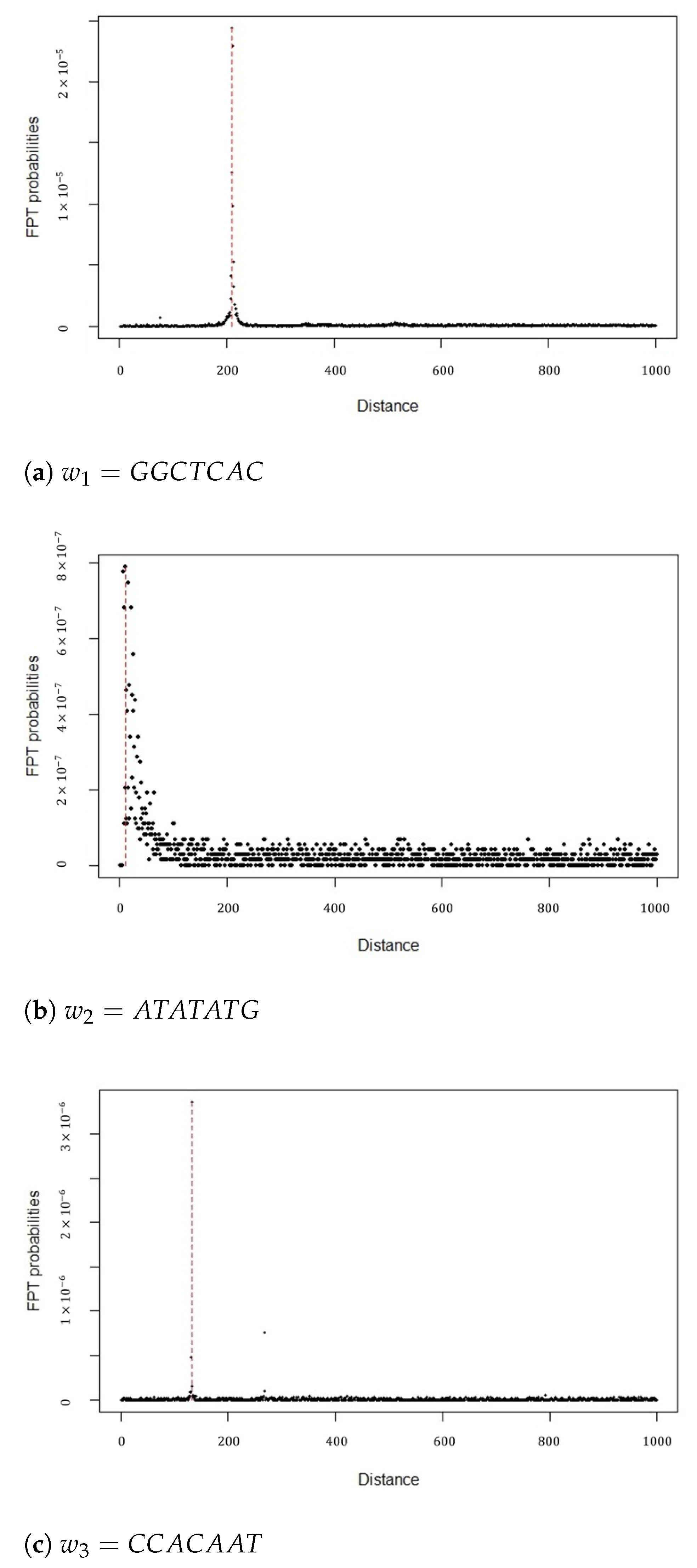
For each DNA word w, there exists a reversed complement of the word $w^{\prime }$. For example, the word $w=ACG$ has the word $w^{\prime }=CGT$ as an inverted repeat. The main question that we will attempt to address by applying the analytic relationships derived earlier is the following: Given that the SMC entered at the initial position in the word w, we want to estimate the probability of the reversed complement word $w^{\prime }$ appearing for the first time after a certain range of letters n. We define the distance, d, between two words as the number of letters between the first letter of the initial word that has appeared and the first letter of the following word that subsequently appears. For the sake of simplicity, we consider only the scenario where $d>l$. The DNA sequence that was used for this illustration is the first chromosome of the human genome consisting of 248,956,422 base-pairs that are publicly available from the website of the National Center for Biotechnology Information (NCBI) [50].

For the first illustration, three words of length $l=7$ were chosen that have been previously shown to exhibit different distances between them and their inverted complements [51]. The words were $w_1=GGCTCAC$, $w_2=ATATATG$ and $w_3=CCACAAT$. For each word, the state space of the SMC consisted of the word and its reversed complement, e.g., $S=\{w_i,w_i^{\prime }\}$. First, the basic parameters of the SMC were estimated, namely the transition probability matrix and the sequence of sojourn times. The sojourn time was defined as the distance, i.e., the number of nucleotides that occur between each word and its inverted repeat. The transition matrix and the empirical distribution of the sojourn times were estimated using the empirical estimators. The sequence of the core matrices was calculated as the Hadamard product of the transition matrix with the sequence of the sojourn time matrices. For each word $w\in S$, the first passage time probability was calculated between the word w and its reversed complement $w^{\prime }$ according to the proposed analytic relationship (Theorem 1). For a maximum distance, ($n=1000$), the highest first passage time probabilities of the three words and their inverted repeats, along with the corresponding distances are illustrated in Figure 1. Concretely, the first passage time probabilities were calculated for the human Chromosome 1, aiming to estimate the most probable distances between words and their symmetrical complements. More specifically, as presented in Figure 1, we have noted that, for the first passage time probabilities, we have $\mathit{arg}max\left(f_{w_1{w}_1^{\prime }}\right)=210$, $\mathit{arg}max\left(f_{w_2{w}_2^{\prime }}\right)=10$ and $\mathit{arg}max\left(f_{w_3{w}_3^{\prime }}\right)=132$ approximating the numerical results of previous studies with corresponding values for the arguments $210,15$ and 133 for the three words, respectively [51]. This highlights the fact that specific DNA words exhibit different behaviors and the distance between them and their inverted repeats demonstrates variability.

4.2. CpG Islands

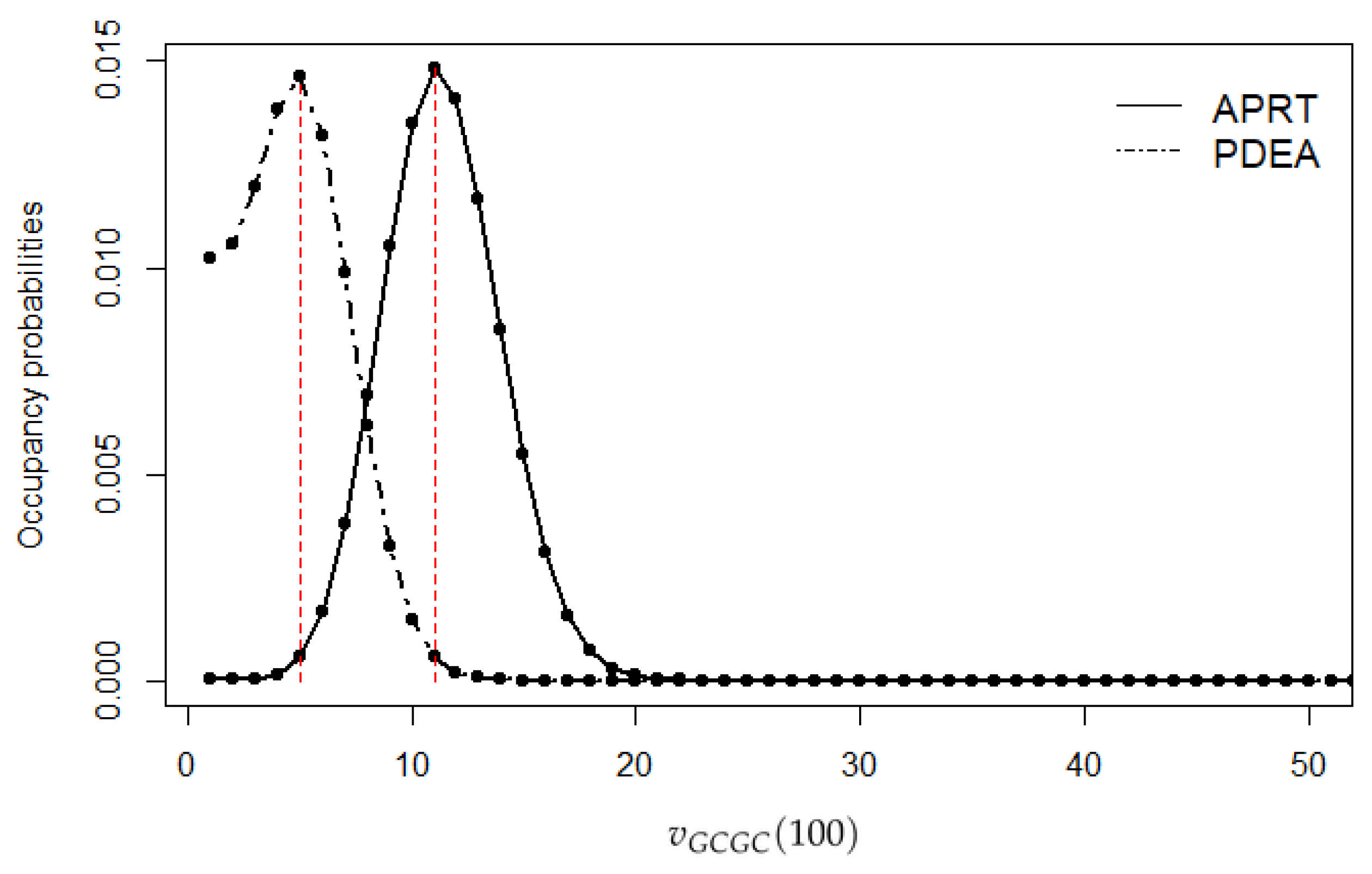
Usually, in vertebrate DNA sequences, the dinucleotide CG occurs less frequently than expected [52]. For the second illustration, we considered CpG islands, which are genomic regions that contain an elevated number of the dinucleotide CG. The human genome contains approximately 30 thousand CpG islands. The APRT gene is an example of a CpG region and it was used for this analysis [53]. This gene provides instructions for making an enzyme called adenine phosphoribosyltransferase (APRT). APRT contains approximately 2500 nucleotides and it had been shown to include an elevated amount of the dinucleotide GC [54]. We modeled the sequence of this DNA region as a homogeneous SMC with state space containing all the two-letter words from the DNA alphabet. The transition probability matrix and the sojourn times were estimated using the empirical estimators. The occupancy distribution ${\omega }_{GCGC}\left(x\right|n)$ for a fixed length of $n=100$ was calculated using the analytic relationship from Theorem 4 in order to estimate the occupancy distribution of specific words up to a specified sequence length. For comparison, we also applied the model to an intron sequence of human’s phosphodiesterase gene (PDEA) [55]. The two sequences are publicly available from the NCBI. The occupancy probabilities are presented in Figure 2 up to length $n=50$. It is confirmed that the number of occupancies of the dinucleotide GC will be greater in the CpG island compared to the intron sequence. As expected, the occupancy probabilities applied on the two sequences indicated that the occurrences of GCs were more frequent in the CpG sequence.

5. Concluding Remarks

In this article, three classes of important probabilities of a semi-Markov process, namely the first passage time, the occupancy and the duration probabilities were defined and their closed analytic forms were proved by using the basic parameters of the process. The study of the first passage time probability provides information regarding the distribution of the time elapsed to reach a state from another for the first time, either in terms of transitions or time. The second category of duration probabilities provides information about the distribution of the number of virtual transitions taking place before an actual transition to a different state occurs. Finally, the third class of probabilities provides insight information regarding the distribution of the number of times the SMC makes transitions to some state in a time interval of a given length. We provided analytic forms on the actual behavior of the recursive relations of the aforementioned probabilities and included these results into specific propositions and theorems.

The analytical results were accompanied with two illustrations on human genome DNA strands which are often studied using probabilistic modeling and, specifically, Markovian models. Although, in the relevant literature, there exist several algorithmic approaches analyzing the occupancy and appearance of words in DNA sequences, the results of the illustration section strongly suggest that the proposed modeling framework could also be used for the investigation of the structure of genome sequences.

Of course nothing comes without limitations and motivation for further research. For example, additional research effort could aim towards high-order dependencies since DNA sequences often show long-range correlations. This could result in a more coherent modeling approach. Furthermore, additional parameters could be included in the model, for example the length of sequence or specific mutations, resulting in more realistic representations regarding the different structures of complex genome of humans and other organisms. Finally, the proposed model could be applied in completely different contexts, such as natural language processing, linguistics, text similarity and anomaly detection, i.e., areas of machine learning that appear to be amongst the most popular areas in the last decade in data science and stochastic modeling.

References

- Pyke, R. Markov renewal processes with finitely many states. Ann. Math. Stat. 1961, 32, 1243–1259. [Google Scholar] [CrossRef]
- Cinlar, E. Introduction to Stochastic Processes; Courier Corporation: Chelmsford, MA, USA, 2013. [Google Scholar]
- Howard, R.A. Dynamic Probabilistic Systems: Semi-Markov and Decision Processes; Dover Publications: Mineola, NY, USA, 2007; Volume 2. [Google Scholar]
- McClean, S.I. A semi-Markov model for a multigrade population with Poisson recruitment. J. Appl. Probab. 1980, 17, 846–852. [Google Scholar] [CrossRef]
- McClean, S.I. Semi-Markov models for manpower planning. In Semi-Markov Models; Springer: Berlin/Heidelberg, Germany, 1986; pp. 283–300. [Google Scholar]
- D’Amico, G.; Di Biase, G.; Janssen, J.; Manca, R. Semi-Markov Migration Models for Credit Risk; Wiley Online Library: Hoboken, NJ, USA, 2017. [Google Scholar]
- Vassiliou, P.-C.G. Non-Homogeneous Semi-Markov and Markov Renewal Processes and Change of Measure in Credit Risk. Mathematics 2021, 9, 55. [Google Scholar] [CrossRef]
- Janssen, J.; Manca, R. Applied Semi-Markov Processes; Springer Science & Business Media: Berlin/Heidelberg, Germany, 2006. [Google Scholar]
- Janssen, J. Semi-Markov Models: Theory and Applications; Springer Science & Business Media: Berlin/Heidelberg, Germany, 2013. [Google Scholar]
- Schbath, S.; Prum, B.; de Turckheim, E. Exceptional motifs in different Markov chain models for a statistical analysis of DNA sequences. J. Comput. Biol. 1995, 2, 417–437. [Google Scholar] [CrossRef]
- De Dominicis, R.; Manca, R. Some new results on the transient behaviour of semi-Markov reward processes. Methods Oper. Res. 1986, 53, 387–397. [Google Scholar]
- Vasileiou, A.; Vassiliou, P.-C.G. An inhomogeneous semi-Markov model for the term structure of credit risk spreads. Adv. Appl. Probab. 2006, 38, 171–198. [Google Scholar] [CrossRef]
- Vassiliou, P.-C.G.; Vasileiou, A. Asymptotic behaviour of the survival probabilities in an inhomogeneous semi-Markov model for the migration process in credit risk. Linear Algebra Appl. 2013, 438, 2880–2903. [Google Scholar] [CrossRef]
- Vassiliou, P.-C.G. Semi-Markov migration process in a stochastic market in credit risk. Linear Algebra Appl. 2014, 450, 13–43. [Google Scholar] [CrossRef]
- Vassiliou, P.-C.G.; Papadopoulou, A. Non-homogeneous semi-Markov systems and maintainability of the state sizes. J. Appl. Probab. 1992, 29, 519–534. [Google Scholar] [CrossRef]
- Vassiliou, P.-C.G. Asymptotic behavior of Markov systems. J. Appl. Probab. 1982, 19, 851–857. [Google Scholar] [CrossRef]
- Dimitriou, V.; Georgiou, A.C. Introduction, analysis and asymptotic behavior of a multi-level manpower planning model in a continuous time setting under potential department contraction. Commun. Stat. Theory Methods 2021, 50, 1173–1199. [Google Scholar] [CrossRef]
- Papadopoulou, A.; Vassiliou, P.-C.G. Asymptotic behavior of nonhomogeneous semi-Markov systems. Linear Algebra Appl. 1994, 210, 153–198. [Google Scholar] [CrossRef] [Green Version]
- Papadopoulou, A.; Vassiliou, P.-C.G. On the variances and convariances of the duration state sizes of semi-Markov systems. Commun. Stat. Theory Methods 2014, 43, 1470–1483. [Google Scholar] [CrossRef]
- Vassiliou, P.-C.G. Markov systems in a general state space. Commun. Stat. Theory Methods 2014, 43, 1322–1339. [Google Scholar] [CrossRef]
- Dimitriou, V.A.; Georgiou, A.C.; Tsantas, N. The multivariate non-homogeneous Markov manpower system in a departmental mobility framework. Eur. J. Oper. Res. 2013, 228, 112–121. [Google Scholar] [CrossRef]
- Symeonaki, M. Theory of fuzzy non homogeneous Markov systems with fuzzy states. Qual. Quant. 2015, 49, 2369–2385. [Google Scholar] [CrossRef]
- Tsaklidis, G.; Vassiliou, P.-C.G. Asymptotic periodicity of the variances and covariances of the state sizes in non-homogeneous Markov systems. J. Appl. Probab. 1988, 25, 21–33. [Google Scholar] [CrossRef]
- Vassiliou, P.-C.G. The evolution of the theory of non-homogeneous Markov systems. Appl. Stoch. Model. Data Anal. 1997, 13, 159–176. [Google Scholar] [CrossRef]
- Vassiliou, P.-C.G.; Georgiou, A.C. Asymptotically attainable structures in nonhomogeneous Markov systems. Oper. Res. 1990, 38, 537–545. [Google Scholar] [CrossRef]
- Ugwuowo, F.I.; McClean, S.I. Modelling heterogeneity in a manpower system: A review. Appl. Stoch. Model. Bus. Ind. 2000, 16, 99–110. [Google Scholar] [CrossRef]
- Symeonaki, M.; Stamatopoulou, G. Describing labour market dynamics through Non Homogeneous Markov System theory. In Demography of Population Health, Aging and Health Expenditures; Springer: Berlin/Heidelberg, Germany, 2020; pp. 359–373. [Google Scholar]
- Ossai, E.; Uche, P. Maintainability of departmentalized manpower structures in Markov chain model. Pac. J. Sci. Technol. 2009, 2, 295–302. [Google Scholar]
- Guerry, M.A.; De Feyter, T. Optimal recruitment strategies in a multi-level manpower planning model. J. Oper. Res. Soc. 2012, 63, 931–940. [Google Scholar] [CrossRef]
- Hunter, J.J. Stationary distributions and mean first passage times of perturbed Markov chains. Linear Algebra Appl. 2005, 410, 217–243. [Google Scholar] [CrossRef] [Green Version]
- Hunter, J.J. Simple procedures for finding mean first passage times in Markov chains. Asia-Pac. J. Oper. Res. 2007, 24, 813–829. [Google Scholar] [CrossRef] [Green Version]
- Hunter, J.J. The computation of the mean first passage times for Markov chains. Linear Algebra Appl. 2018, 549, 100–122. [Google Scholar] [CrossRef] [Green Version]
- Yao, D.D. First-passage-time moments of Markov processes. J. Appl. Probab. 1985, 22, 939–945. [Google Scholar] [CrossRef]
- Zhang, X.; Hou, Z. The first-passage times of phase semi-Markov processes. Stat. Probab. Lett. 2012, 82, 40–48. [Google Scholar] [CrossRef]
- Pitman, J.; Tang, W. Tree formulas, mean first passage times and Kemeny’s constant of a Markov chain. Bernoulli 2018, 24, 1942–1972. [Google Scholar] [CrossRef] [Green Version]
- Redner, S. A Guide to First-Passage Processes; Cambridge University Press: Cambridge, UK, 2001. [Google Scholar]
- Waterman, M.S. Introduction to Computational Biology: Maps, Sequences and Genomes; CRC Press: Boca Raton, FL, USA, 1995. [Google Scholar]
- Almagor, H. A Markov analysis of DNA sequences. J. Theor. Biol. 1983, 104, 633–645. [Google Scholar] [CrossRef]
- Menéndez, M.; Pardo, L.; Pardo, M.; Zografos, K. Testing the order of Markov dependence in DNA sequences. Methodol. Comput. Appl. Probab. 2011, 13, 59–74. [Google Scholar] [CrossRef]
- Skewes, A.D.; Welch, R.D. A Markovian analysis of bacterial genome sequence constraints. PeerJ 2013, 1, e127. [Google Scholar] [CrossRef] [PubMed]
- Papapetrou, M.; Kugiumtzis, D. Markov chain order estimation with conditional mutual information. Phys. A: Stat. Mech. Appl. 2013, 392, 1593–1601. [Google Scholar] [CrossRef] [Green Version]
- Boys, R.J.; Henderson, D.A.; Wilkinson, D.J. Detecting homogeneous segments in DNA sequences by using hidden Markov models. J. R. Stat. Soc. Ser. C 2000, 49, 269–285. [Google Scholar] [CrossRef]
- Reinert, G.; Schbath, S.; Waterman, M.S. Probabilistic and statistical properties of words: An overview. J. Comput. Biol. 2000, 7, 1–46. [Google Scholar] [CrossRef] [Green Version]
- Robin, S.; Daudin, J.J. Exact distribution of word occurrences in a random sequence of letters. J. Appl. Probab. 1999, 36, 179–193. [Google Scholar] [CrossRef]
- Schbath, S. An overview on the distribution of word counts in Markov chains. J. Comput. Biol. 2000, 7, 193–201. [Google Scholar] [CrossRef]
- Papadopoulou, A. Some Results on Modeling Biological Sequences and Web Navigation with a Semi Markov Chain. Commun. Stat. Theory Methods 2013, 42, 2853–2871. [Google Scholar] [CrossRef]
- Ricciardi, L.; Crescenzo, A.; Giorno, V.; Nobile, A. An outline of theoretical and algorithmic approaches to first passage time problems with applications to biological modeling. Math. Jpn. 1999, 50, 247–322. [Google Scholar]
- Lavi, B.; Levy Karin, E.; Pupko, T.; Hazkani-Covo, E. The prevalence and evolutionary conservation of inverted repeats in proteobacteria. Genome Biol. Evol. 2018, 10, 918–927. [Google Scholar] [CrossRef] [Green Version]
- Brázda, V.; Laister, R.C.; Jagelská, E.B.; Arrowsmith, C. Cruciform structures are a common DNA feature important for regulating biological processes. BMC Mol. Biol. 2011, 12, 1–16. [Google Scholar] [CrossRef] [Green Version]
- Homo Sapiens Chromosome 1, GRCh38.p13 Primary Assembly. Available online: https://www.ncbi.nlm.nih.gov/nuccore/CM000663 (accessed on 17 December 2020).
- Tavares, A.H.; Pinho, A.J.; Silva, R.M.; Rodrigues, J.M.; Bastos, C.A.; Ferreira, P.J.; Afreixo, V. DNA word analysis based on the distribution of the distances between symmetric words. Sci. Rep. 2017, 7, 1–11. [Google Scholar] [CrossRef] [PubMed] [Green Version]
- Gardiner-Garden, M.; Frommer, M. CpG islands in vertebrate genomes. J. Mol. Biol. 1987, 196, 261–282. [Google Scholar] [CrossRef]
- APRT adenine phosphoribosyltransferase. Available online: https://www.ncbi.nlm.nih.gov/gtr/genes/353/ (accessed on 17 December 2020).
- Broderick, T.P.; Schaff, D.A.; Bertino, A.M.; Dush, M.K.; Tischfield, J.A.; Stambrook, P.J. Comparative anatomy of the human APRT gene and enzyme: Nucleotide sequence divergence and conservation of a nonrandom CpG dinucleotide arrangement. Proc. Natl. Acad. Sci. USA 1987, 84, 3349–3353. [Google Scholar] [CrossRef] [PubMed] [Green Version]
- Homo sapiens Human Phosphodiesterase (PDEA) Gene. Available online: https://www.ncbi.nlm.nih.gov/nuccore/1059792111 (accessed on 17 December 2020).
- Farmakioti, E. Probabilities of State Occupancies in Semi-Markov Chains. Master’s Thesis, Aristotle University of Thessaloniki, Thessaloniki, Greece, 2018. [Google Scholar]
Figure 1.
First passage time (FPT) probabilities for distance n ≤ 1000.
Figure 2.
Occupancy probabilities of APRT and PDEA genes.
Publisher’s Note: MDPI stays neutral with regard to jurisdictional claims in published maps and institutional affiliations. |
© 2021 by the authors. Licensee MDPI, Basel, Switzerland. This article is an open access article distributed under the terms and conditions of the Creative Commons Attribution (CC BY) license (https://creativecommons.org/licenses/by/4.0/).
Share and Cite
MDPI and ACS Style
Georgiou, A.C.; Papadopoulou, A.; Kolias, P.; Palikrousis, H.; Farmakioti, E. On State Occupancies, First Passage Times and Duration in Non-Homogeneous Semi-Markov Chains. Mathematics 2021, 9, 1745. https://doi.org/10.3390/math9151745
AMA Style
Georgiou AC, Papadopoulou A, Kolias P, Palikrousis H, Farmakioti E. On State Occupancies, First Passage Times and Duration in Non-Homogeneous Semi-Markov Chains. Mathematics. 2021; 9(15):1745. https://doi.org/10.3390/math9151745
Chicago/Turabian StyleGeorgiou, Andreas C., Alexandra Papadopoulou, Pavlos Kolias, Haris Palikrousis, and Evanthia Farmakioti. 2021. "On State Occupancies, First Passage Times and Duration in Non-Homogeneous Semi-Markov Chains" Mathematics 9, no. 15: 1745. https://doi.org/10.3390/math9151745
Note that from the first issue of 2016, this journal uses article numbers instead of page numbers. See further details here.