
MHD Laminar Boundary Layer Flow of a Jeffrey Fluid Past a Vertical Plate Influenced by Viscous Dissipation and a Heat Source/Sink


1
Department of Mathematics and Computational Sciences, Faculty of Science, University of Zimbabwe, Mt. Pleasant, Harare P.O. Box MP167, Zimbabwe
2
Department of Mathematics and Applied Mathematics, School of Natural and Mathematical Sciences, University of Venda, P. Bag X5050, Thohoyandou 0950, South Africa
*
Author to whom correspondence should be addressed.
Mathematics 2021, 9(16), 1896; https://doi.org/10.3390/math9161896
Submission received: 16 June 2021
/
Revised: 22 July 2021
/
Accepted: 28 July 2021
/
Published: 9 August 2021
(This article belongs to the Special Issue New Trends and Developments in Numerical Analysis)
Abstract
:This study investigates the effects of viscous dissipation and a heat source or sink on the magneto-hydrodynamic laminar boundary layer flow of a Jeffrey fluid past a vertical plate. The governing boundary layer non-linear partial differential equations are reduced to non-linear ordinary differential equations using suitable similarity transformations. The resulting system of dimensionless differential equations is then solved numerically using the bivariate spectral quasi-linearisation method. The effects of some physical parameters that include the Schmidt number, Eckert number, radiation parameter, magnetic field parameter, heat generation parameter, and the ratio of relaxation to retardation times on the velocity, temperature, and concentration profiles are presented graphically. Additionally, the influence of some physical parameters on the skin friction coefficient, local Nusselt number, and the local Sherwood number are displayed in tabular form.
1. Introduction
The study of fluids, either stationary or in motion has vast applications in science, biology, physiology, medicine, and engineering. Basically, fluids can be grouped into two classes, Newtonian and non-Newtonian fluids. Newtonian fluids are those fluids that obey Newton’s law of viscosity. Those fluids that deviate from the law are said to be non-Newtonian. Typical non-Newtonian fluids include blood, saliva, starch solutions, toothpaste, and sauces. Due to the fact that non-Newtonian fluids cannot be described by a single constitutive equation like the Navier–Stokes equations, they tend to be more complicated than Newtonian fluids. Although complicated, non-Newtonian fluids have found more industrial applications than Newtonian fluids. Recently, there is much attention which has been paid on the study of non-Newtonian fluid flow. The non-Newtonian fluids can be characterised as being of the differential, rate or integral type, Cioranescu et al. [1]. Some of the non-Newtonian models which have been studied include the Jeffrey model [2,3], the Maxwell model [4,5], the Oldroyd-B model [6,7], and the Herschel–Bulkley model [8,9].
One non-Newtonian fluid model of interest in this study is the Jeffrey model which is of the rate type. The Jeffrey fluid expresses the influence of the ratio of relaxation to retardation times and its constitutive equation can be reduced to that of a Newtonian fluid as a special case. Unlike viscous fluid models, the Jeffrey model can be used in non-Newtonian fluids to describe the stress relaxation property, Kahshan et al. [10]. Due to its viscoelastic properties, the Jeffrey fluid has found some industrial applications in polymer productions. The model has recently attracted the attention of many researchers since it gives better approximations to most physiological fluids. The Jeffrey fluid model was successfully used to model the peristaltic flow of chyme in the small intestines by Akbar et al. [11]. Additionally, Sharma et al. [12] used the Jeffrey fluid to model the flow of blood in narrow arteries. Nallapu and Radhakrishnamacharya [13] did an investigation of the effects of a magnetic field in the flow of the Jeffrey fluid in narrow tubes in a porous medium. Some other researches which have been completed on the Jeffrey model include the works by: Ellahi et al. [14], Khan et al. [15], Vaidya et al. [16].
There is quite a substantial amount of research which has been performed on the MHD boundary layer flow of a Jeffrey fluid. A study on magneto-hydrodynamic boundary layer flow of a Jeffrey fluid over a sheet in a porous medium was conducted by Ahmad and Ishak [17]. Nadeem et al. [18] did a numerical study of the laminar boundary layer flow of a Jeffrey fluid in which they investigated the effects of thermal radiation when the fluid is flowing over a surface that stretches exponentially. The homotopy analysis approach was employed by Hayat et al. [19] to study the influence of some embedded parameters on the laminar boundary layer flow of a Jeffrey fluid. Tlili [20] investigated the heat generation and MHD effects on an incompressible two-dimensional laminar boundary layer Jeffrey fluid flow.
Some significant work has been completed on the non-Newtonian fluid flow past a vertical plate. This is attributed to its wide applications in engineering, technology, as well as in the manufacturing industry. Babu et al. [21] considered the influence of the Hall currents in a chemically reactive multivariate Jeffrey fluid which is flowing through a vertical plate. A study on the effects of viscous dissipation on an MHD Jeffrey fluid flowing through a vertical channel was completed by Selvi and Muthuraj [22]. Amanulla et al. [23] discussed the effects of heat transfer in a Jeffrey fluid from an inclined vertical plate. An investigation on the flow of an incompressible non-Newtonian Jeffrey fluid past a vertical porous plate was completed by Prasad et al. [24] using an implicit finite difference method.
The study of flow of non-Newtonian fluids influenced by a heat source or sink has found applications in the disposal of radioactive waste material, food stuffs storage, removal of heat from nuclear fuel debris, and many others, Hayat et al. [25]. Nisar et al. [26] did an analysis of the flow of an electrically conducting fluid flowing over a stretching surface with a uniform heat source. A Cattaneo–Christov model with double stratification, thermal relaxation, and a heat source was used to investigate heat and mass transfer in a Jeffrey fluid by Hussain et al. [27]. Qasim [28] investigated both heat and mass transfer in a Jeffrey fluid flowing over a stretching sheet with a heat source.
In this current work, a numerical technique called the bivariate spectral quasi-linearisation method (BSQLM), Motsa et al. [29], was used to perform a mathematical investigation of the laminar boundary layer flow of a Jeffrey fluid. The non-Newtonian fluid flows past a vertical plate with the flow being influenced by viscous dissipation and a heat source or sink. We intend to implement the BSQLM in this current study as it is reported by Magagula et al. [30] that the method is computationally efficient and gives solutions that are more uniformly accurate than traditional methods like the finite difference methods. Although the BSQLM does not handle periodic boundary conditions properly, the method is considered because it is easy to implement and it takes little time to converge to the exact solution with few grid points, Rai and Mondal [31]. There is quite a number of studies that have been completed in analysing fluid flow problems using the BSQLM. Goqo et al. [32] used the BSQLM to obtain the convergent solutions of the model equations that describe the viscous nanofluid flowing over a porous wedge. Additionally, Motsa and Ansari et al. [33] used the BSQLM to investigate unsteady boundary layer flow of an Oldroyd-B nanofluid towards a stretching sheet with variable thermal conductivity.
2. Problem Statement and Mathematical Formulation
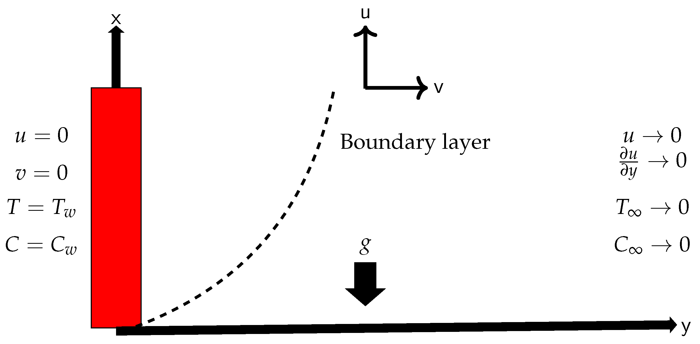
In this study, we consider the magneto-hydrodynamic laminar boundary layer flow of a Jeffrey fluid past a vertical porous plate, with the flow being influenced by viscous dissipation and a heat source or sink. The x-axis is measured along the plate in the upward direction and the y-axis is measured normal to the plate in the outward direction. Initially, both the surface of the plate and the Jeffrey fluid are at rest at a uniform temperature and concentration , respectively. The respective ambient temperature and concentration of the fluid far way from the plate are given by and . The acceleration due to gravity g acts vertically downwards. The geometry of the problem is shown in Figure 1.
The Jeffrey fluid constitutive equation is given by [34,35] as,
where is the extra-stress tensor, is the first Rivlin–Erickson tensor, is the ratio of relaxation to retardation times, is the retardation time and is the viscosity. After incorporating the Jeffrey fluid stress tensor in the momentum equation, the model is given by, Abdul Gaffar et al. [36]
where the velocities in the x and y directions are u and v, respectively. T is the fluid temperature, C is the fluid concentration, is mass diffusivity, is the chemical reaction rate constant, is kinematic viscosity, is the radiative heat flux, is fluid density. Additionally, g, , and are the acceleration due to gravity, thermal expansion coefficient, solutal expansion coefficient, and thermal diffusivity, respectively. The boundary conditions are chosen in such a way that there is no flow across the plate and due to viscosity, there is no slip condition at the plate. These boundary conditions for the temperature, concentration, and velocity are given by:
Under the Rosseland approximation, the radiative heat flux has the form, El-Aziz and Yahya [37]
where is the Stefan–Boltzmann constant and is the mean absorption coefficient. Assuming that the temperature differences within the Jeffrey fluid flow are sufficiently small, Taylor’s series expansion of about gives
Similarity Transformations
The transformation of the system of Equations (4)–(6) into a dimensionless system is achieved by the application of the similarity transformations, Abdul Gaffar et al. [36]:
The similarity transformations defined in Equation (12) when applied to the momentum, energy, and concentration equations yield
where is the chemical reaction parameter, is the radiation parameter, is the concentration to thermal buoyancy ratio, is the Prandtl number, is the Schmidt number, is the magnetic field parameter, is the Eckert number, is the heat generation or absorption parameter and is the Deborah number. The dimensionless boundary conditions take the form
3. Method of Solution
The numerical solutions of the dimensionless system of Equations (13)–(15) subject to boundary conditions (16) are obtained using the BSQLM. The method basically combines the quasi-linearisation method (QLM) and the Chebyshev spectral collocation method (CSCM). The application of a Newton–Raphson based QLM, Alharbey et al. [38], transforms the coupled non-linear differential Equations (13)–(15) into a system of linear iterative differential equations:
The subscripts m and denote the previous and current iteration levels, respectively. The variable coefficients evaluated at the previous iteration level m are expressed as follows:
Additionally, the right hand side terms, evaluated at the current iteration level, are given by the following definitions
The boundary conditions evaluated at the current iteration level are:
In order for us to implement the CSCM on the system of Equations (17)–(19), we move the physical domain on the axis on which Equations (13)–(15) are defined to the computational domain on the axis using linear transformations
truncate the semi-infinite physical domains in the and directions, respectively, such that the infinity boundary conditions hold. Approximations of , and have the following respective forms
where the Lagrange interpolating polynomials are defined as:
Evaluating the differential Equations (17)–(19) at the Chebyshev–Gauss–Lobatto collocation points and and Chebyshev differentiation gives
where and . and are the Chebyshev differentiation matrices, Trefethen [39]. The diagonal matrices
In matrix-vector form, the system of Equations (24)–(26) can be written as
where
and have a similar form as , whilst and take the same form as . When ,
and when
The engineering design quantities of physical interest to be discussed in this work are the skin-friction coefficient which is a measure of shear stress at the plate, the Nusselt number which is a measure of the rate of heat transfer and the Sherwood number which measures the rate of mass transfer at the plate.
4. Results and Discussions
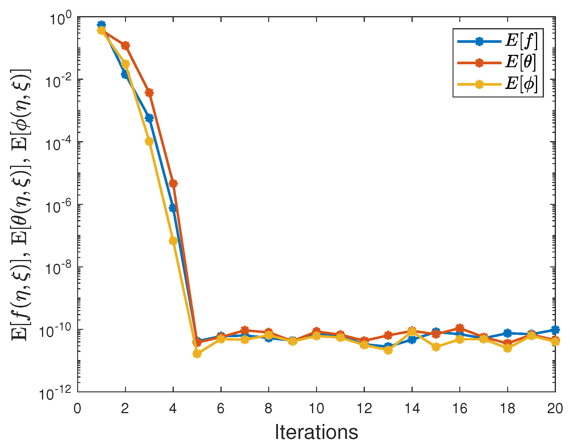
Presented in this section are the numerical results of the BSQLM algorithm for solving MHD laminar boundary layer flow of a Jeffrey fluid past a vertical plate. All the numerical simulations were completed using MATLAB 2020. Unless otherwise stated, the default parameters considered in this work are: , , , , , , , , and . The method was tested for both convergence and accuracy using the infinity norms of both the absolute and residual errors, respectively. The formulae for the convergence error infinity norms are defined as:
Figure 2 displays the convergence error norms plotted against the number of iterations. We can infer that the error norms decrease with increasing number of iterations. This confirms convergence of the method. The residual error infinity norms are given by
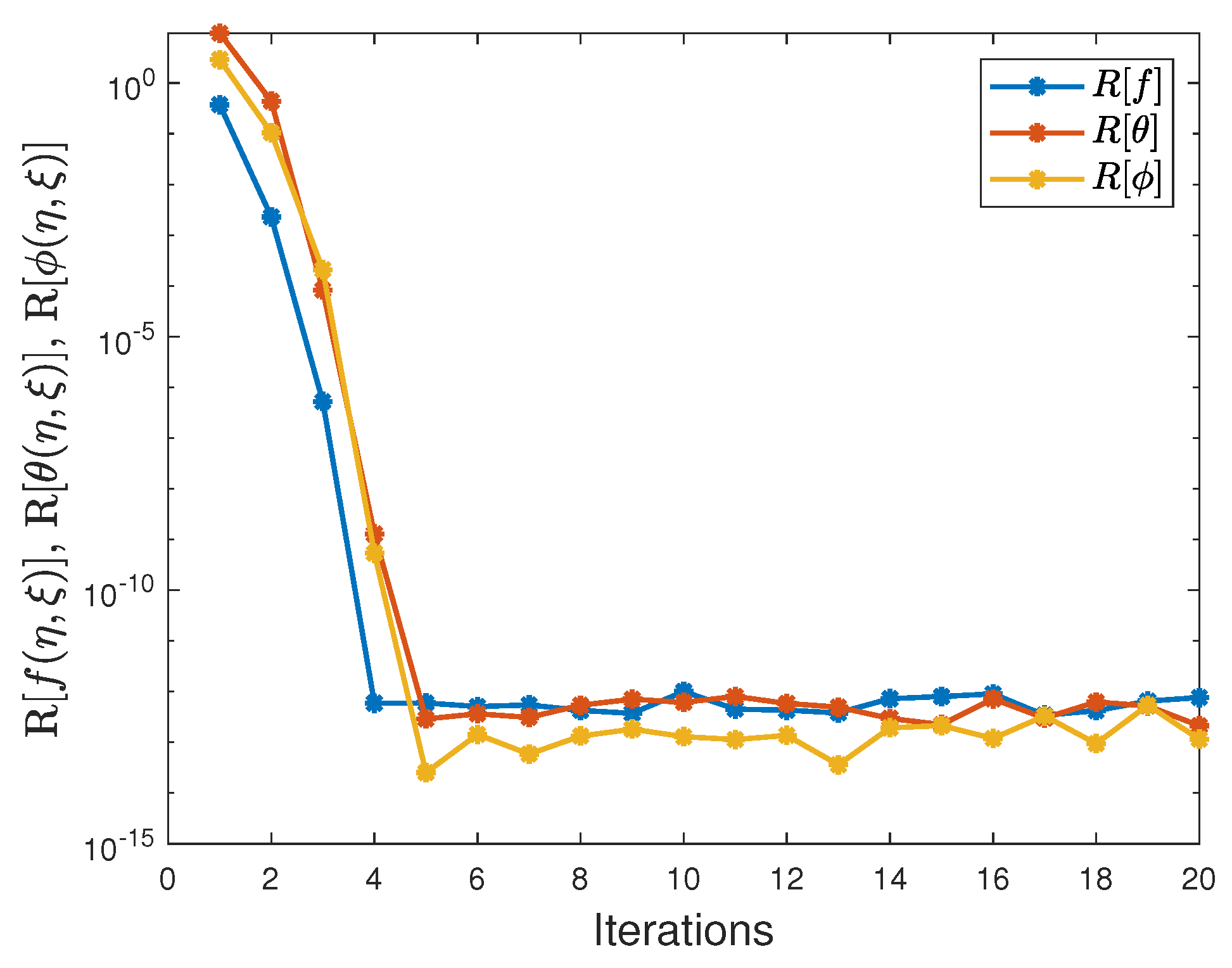
Figure 3 depicts the variation of the residual error infinity norms with the number of iterations. The method achieves an error of about after 5 iterations. This shows that the BSQLM is a very accurate method for solving non-linear differential problems.
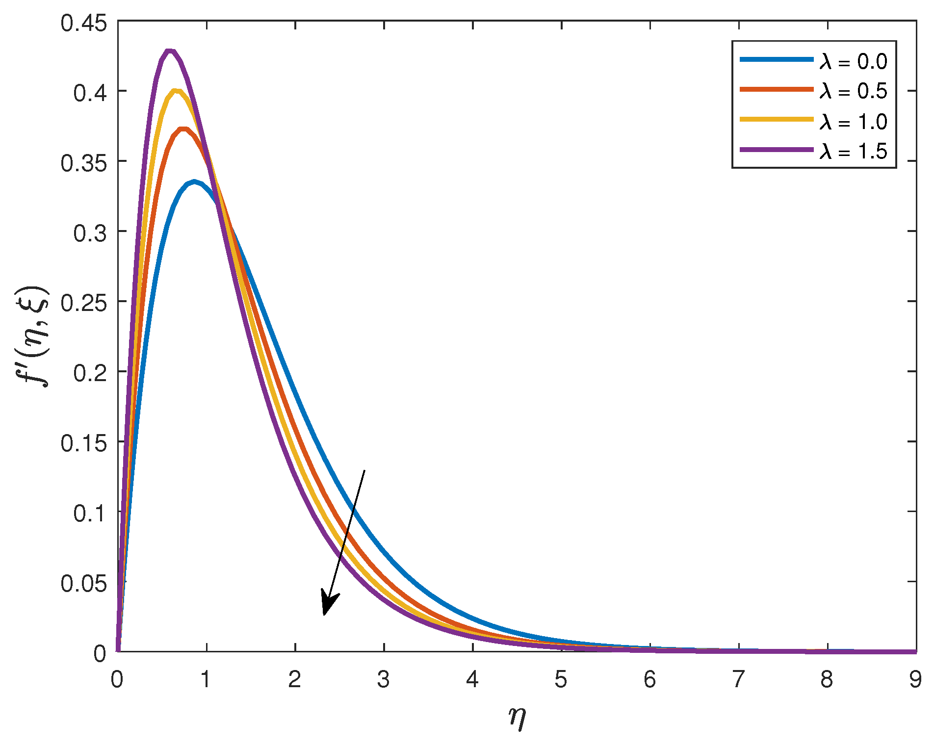
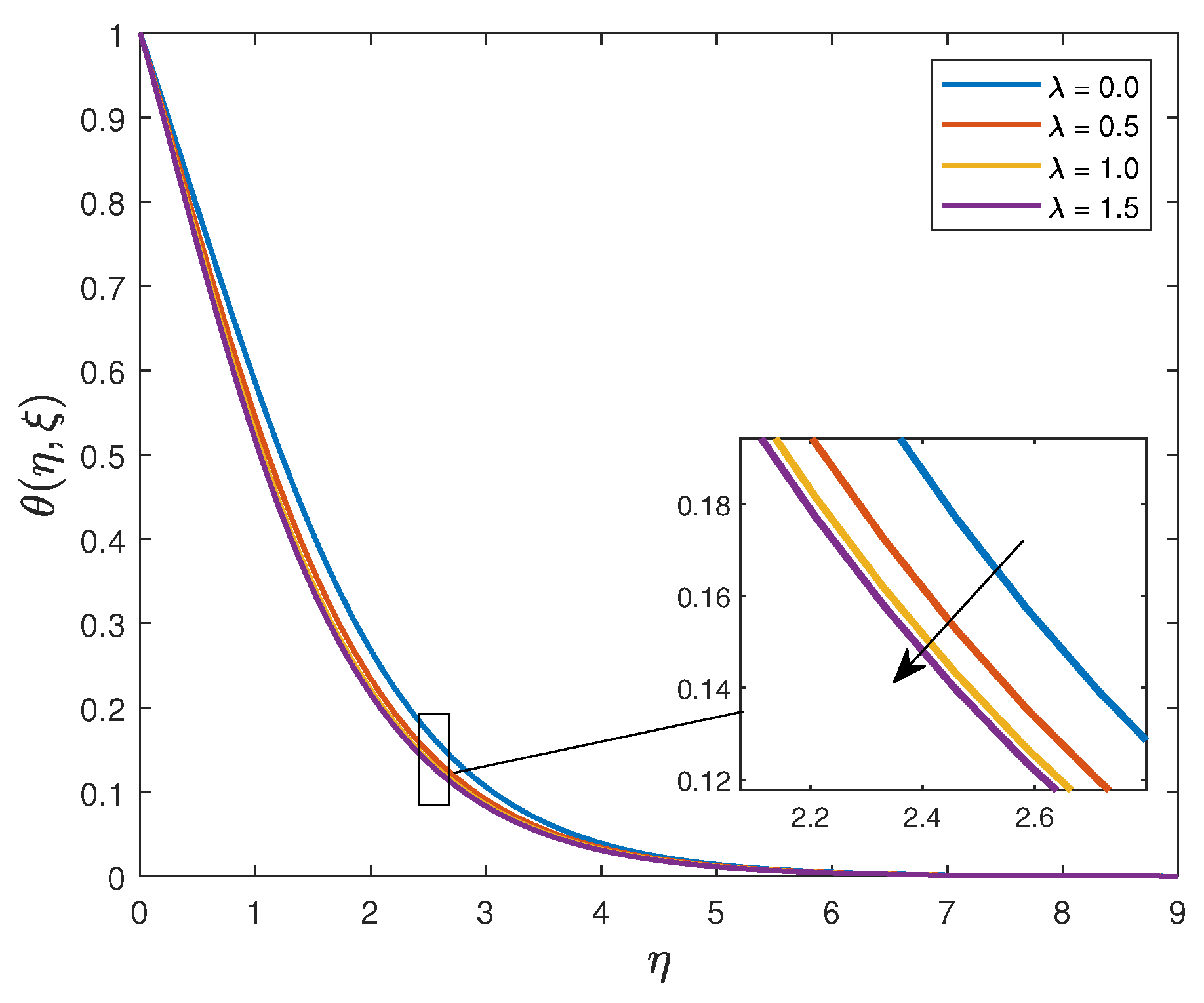
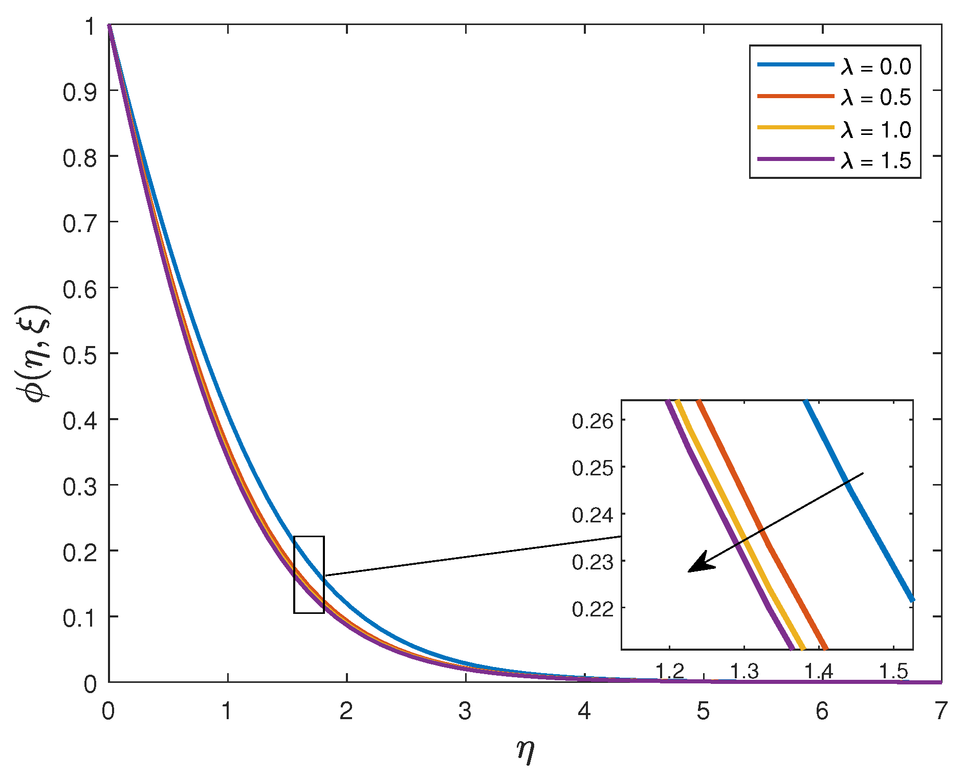
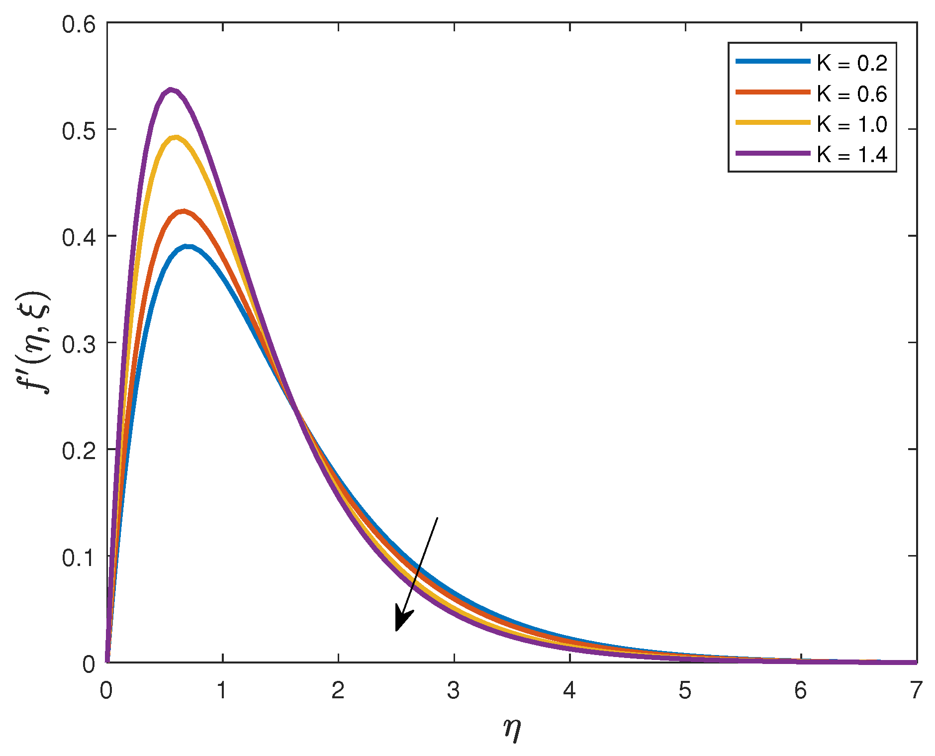
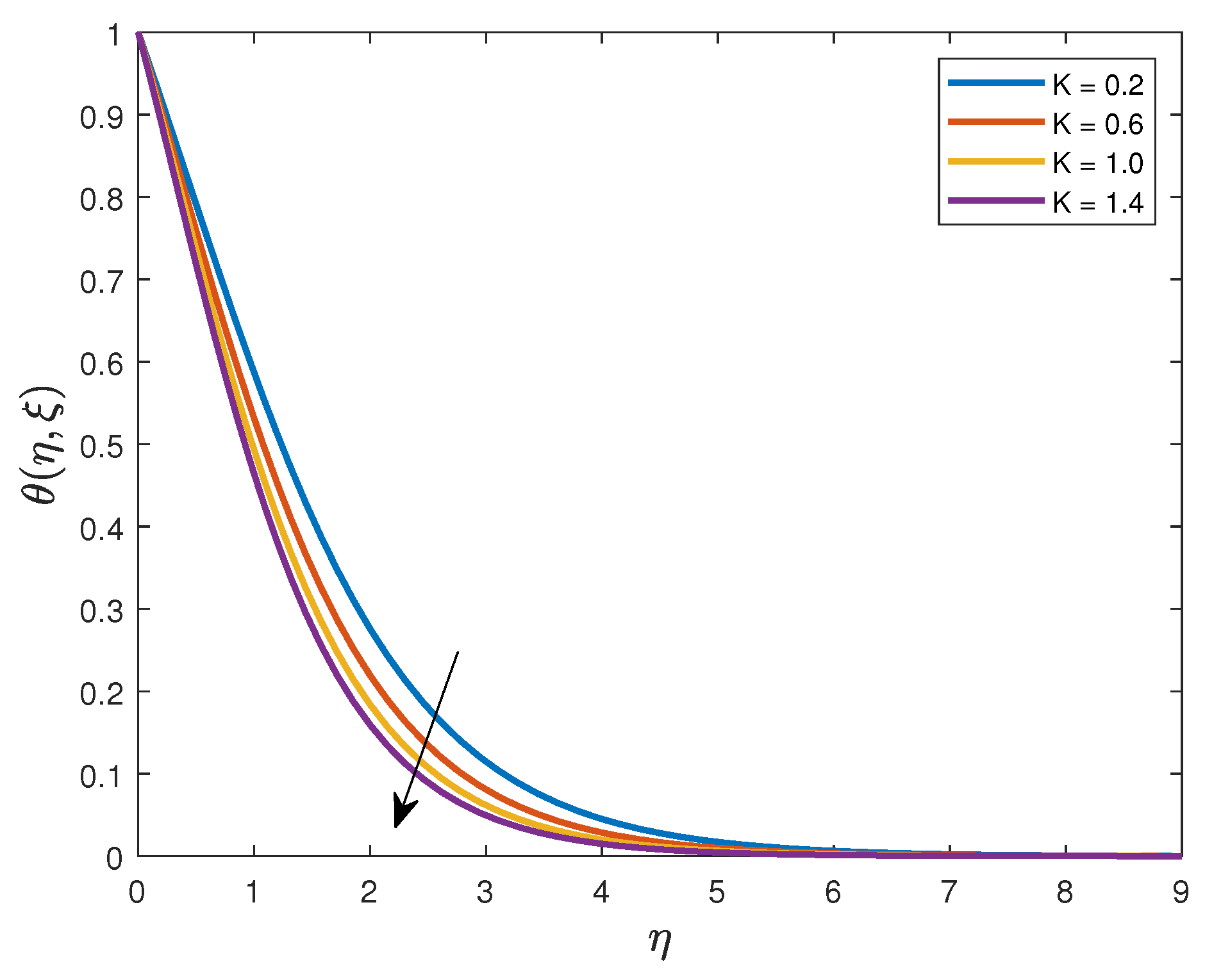
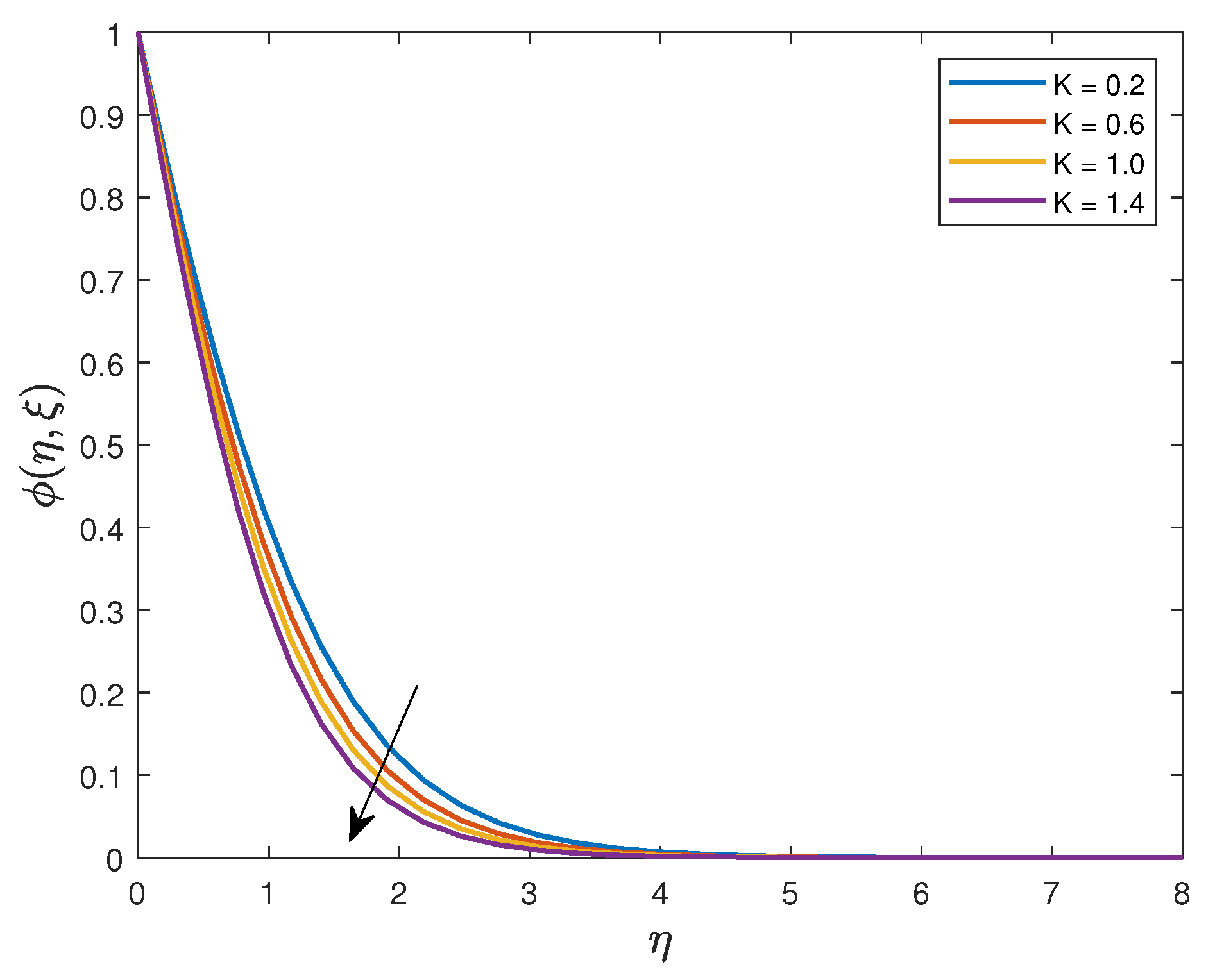
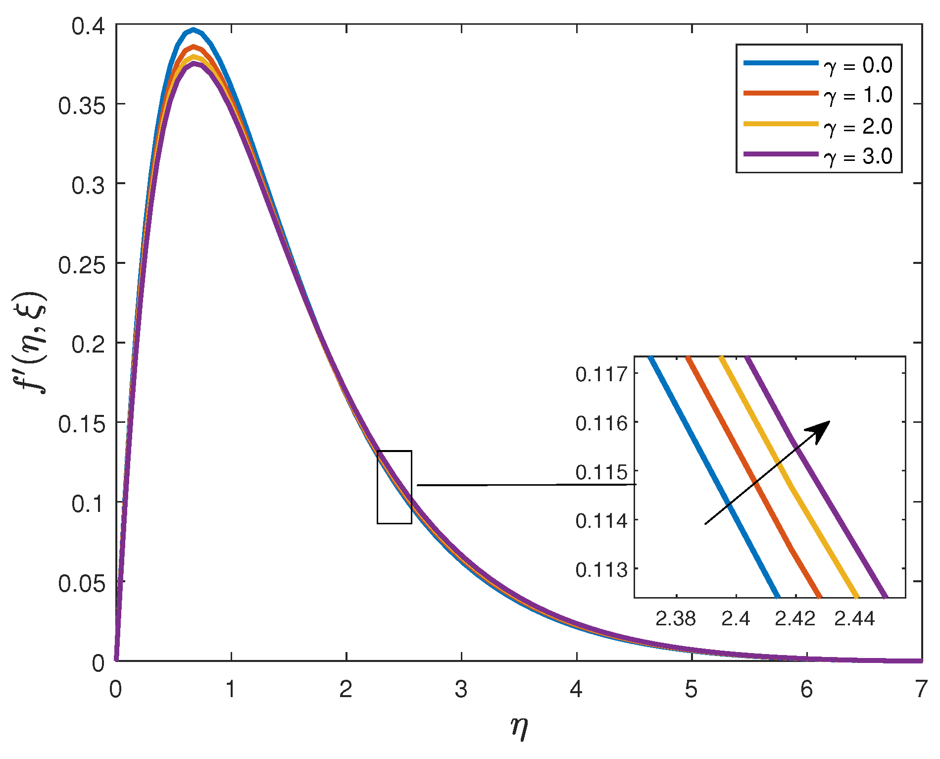
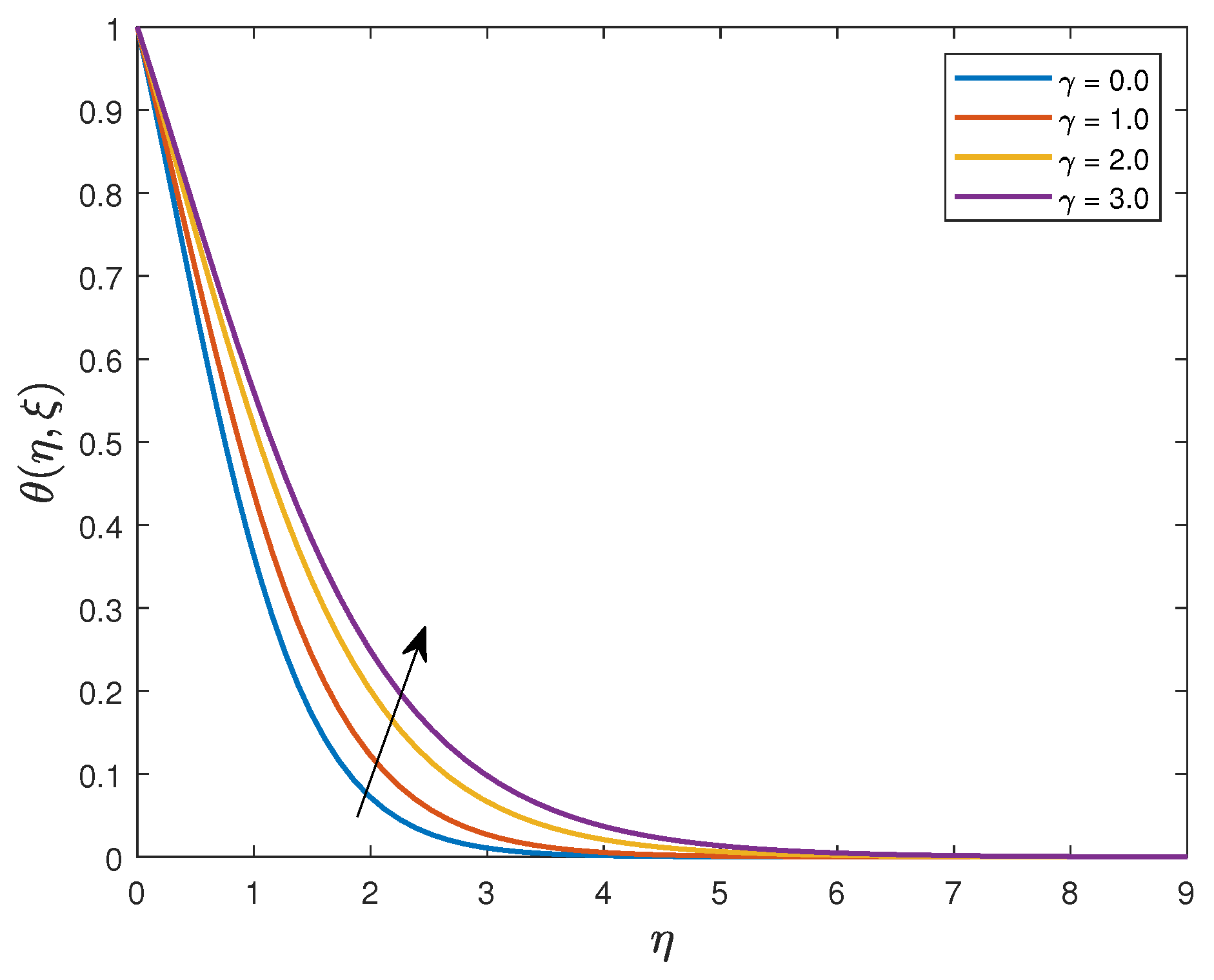
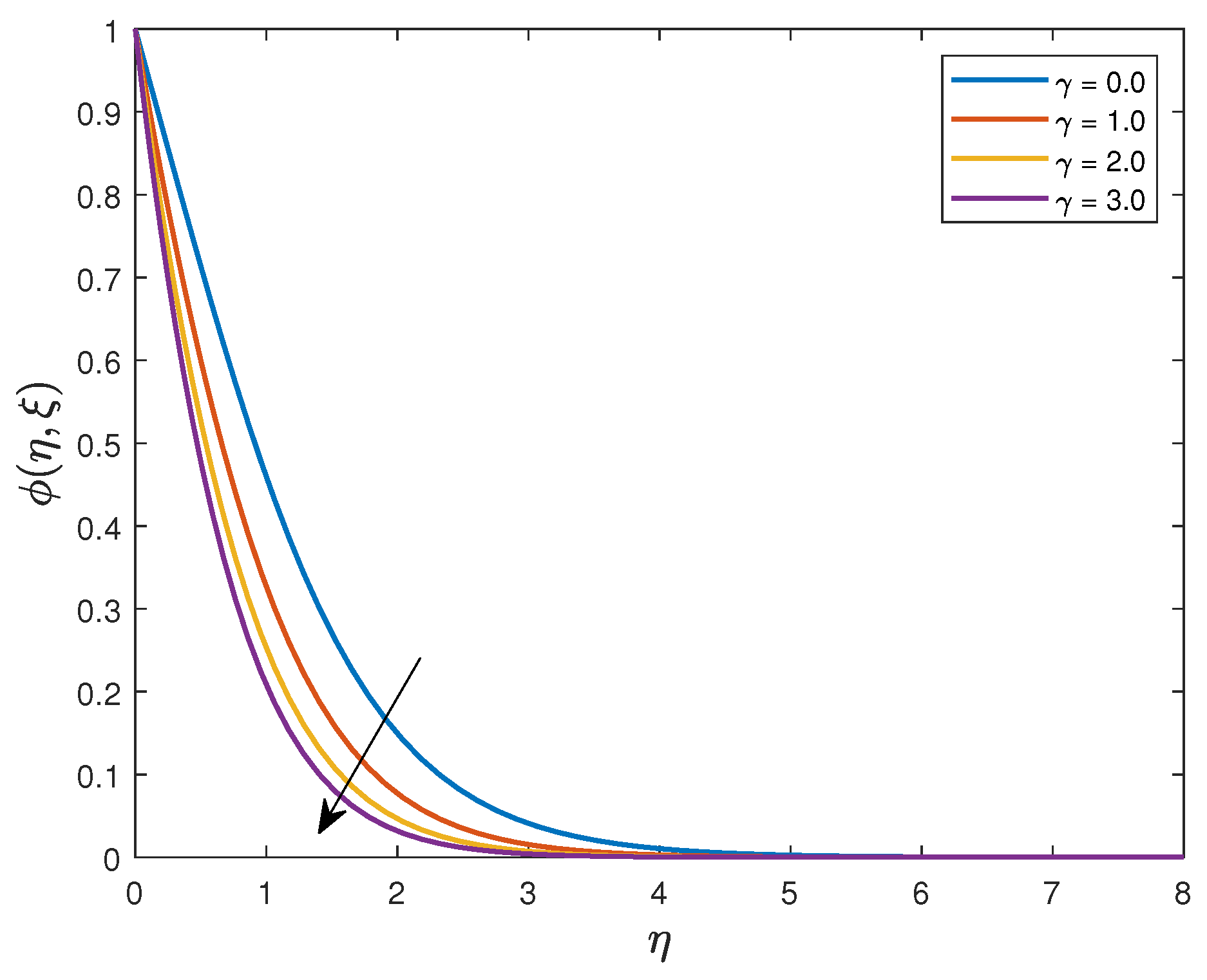
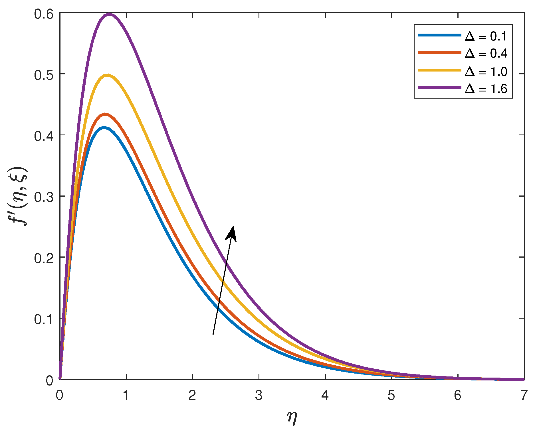
The effects of the ratio of relaxation to retardation times parameter on the fluid velocity, temperature and concentration are depicted in Figure 4, Figure 5 and Figure 6. It is observed that enhancing results in an increase in the fluid velocity near the vertical plate but the velocity decreases towards the free stream. Generally, the fluid temperature and concentration are slightly depressed as is increased. The ratio of relaxation to retardation times is inversely proportional to the retardation time, which is the time the material require to react to deformation. An increase in signifies weaker retardation time. Figure 7, Figure 8 and Figure 9 depict the influence of the concentration to thermal buoyancy parameter K on the fluid velocity, temperature, and concentration. From Figure 7, it is noted that the momentum boundary thickens near the plate and then diminishes as the free-stream is approached. Both the temperature and solute concentration distributions are reduced with increasing K as displayed in Figure 8 and Figure 9.
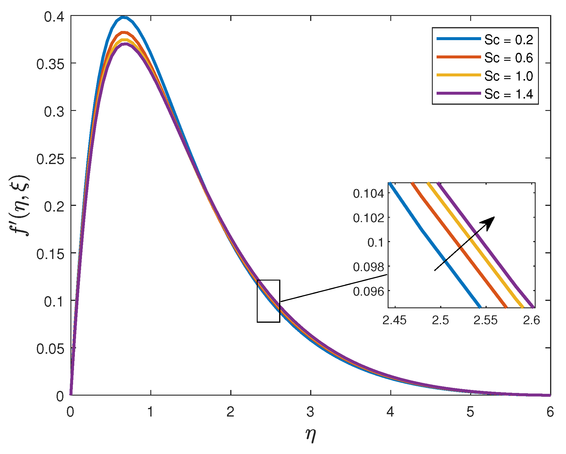
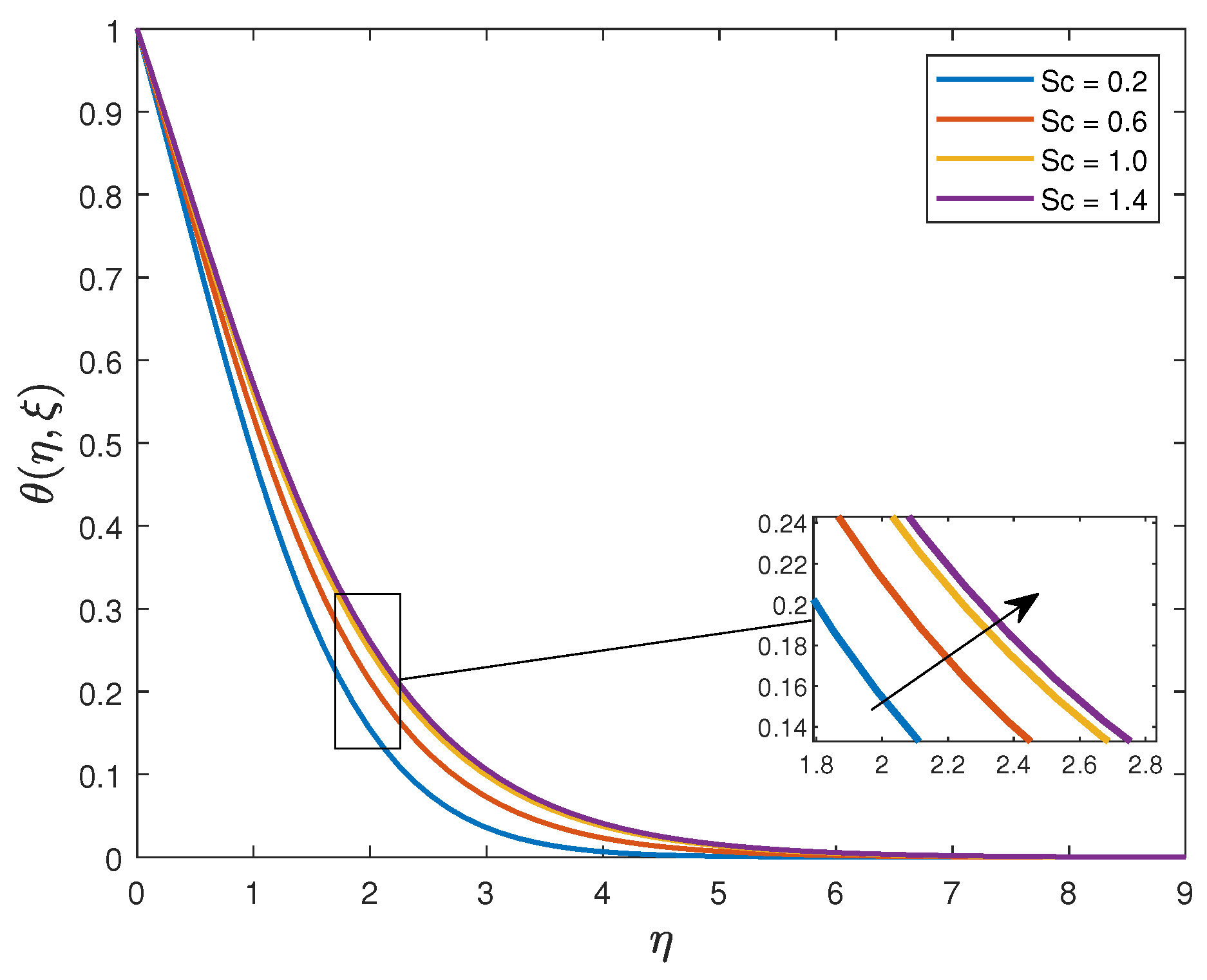
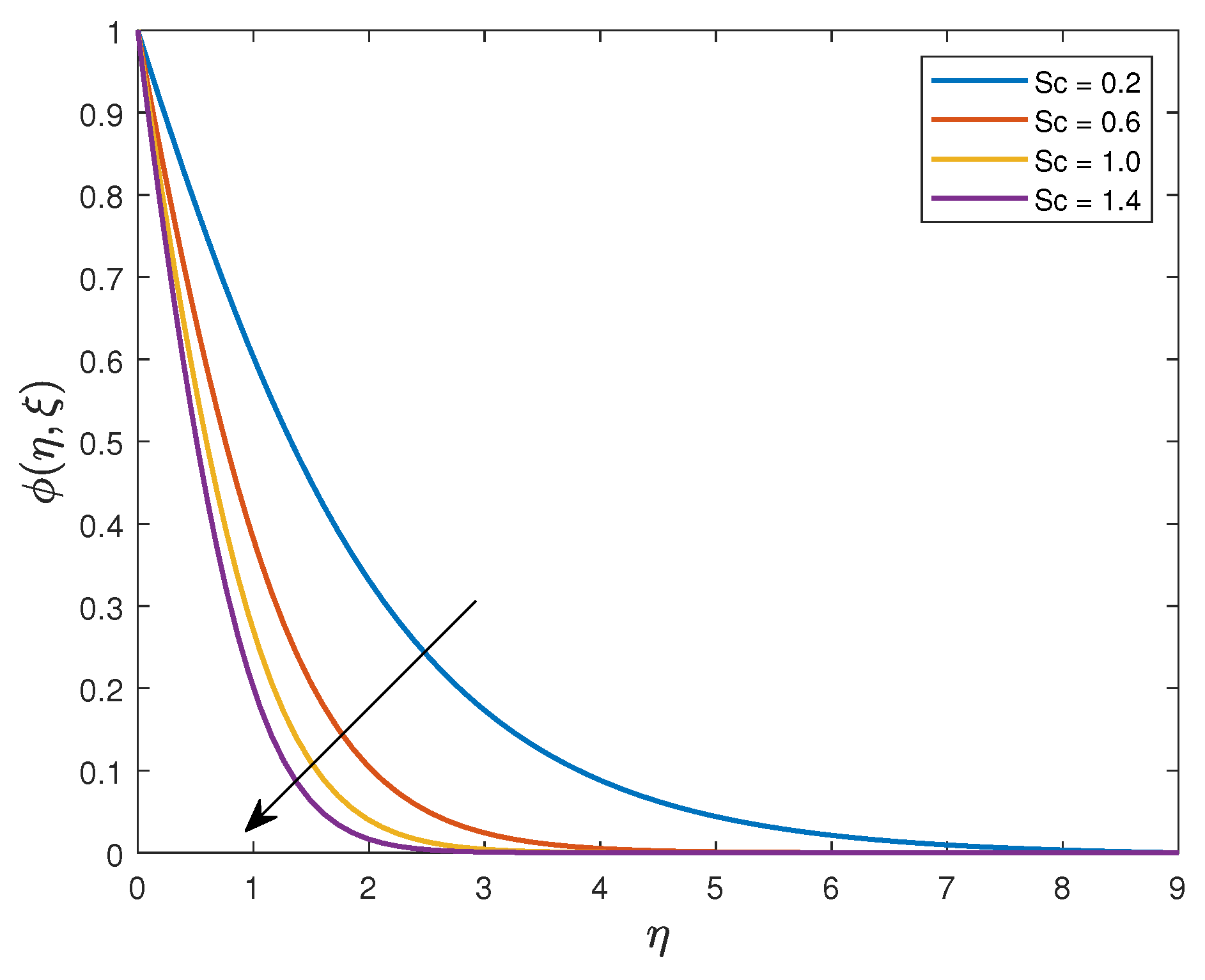
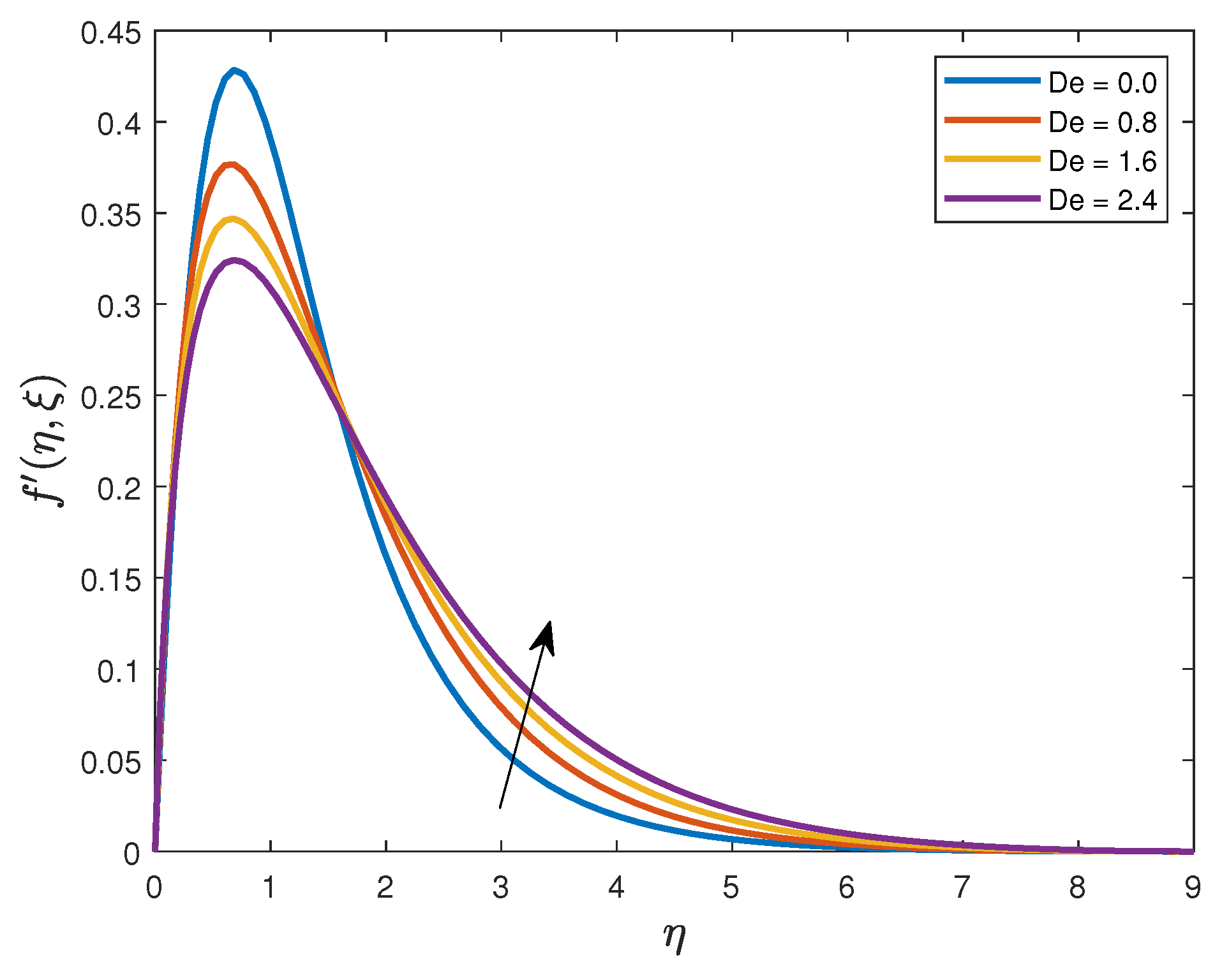
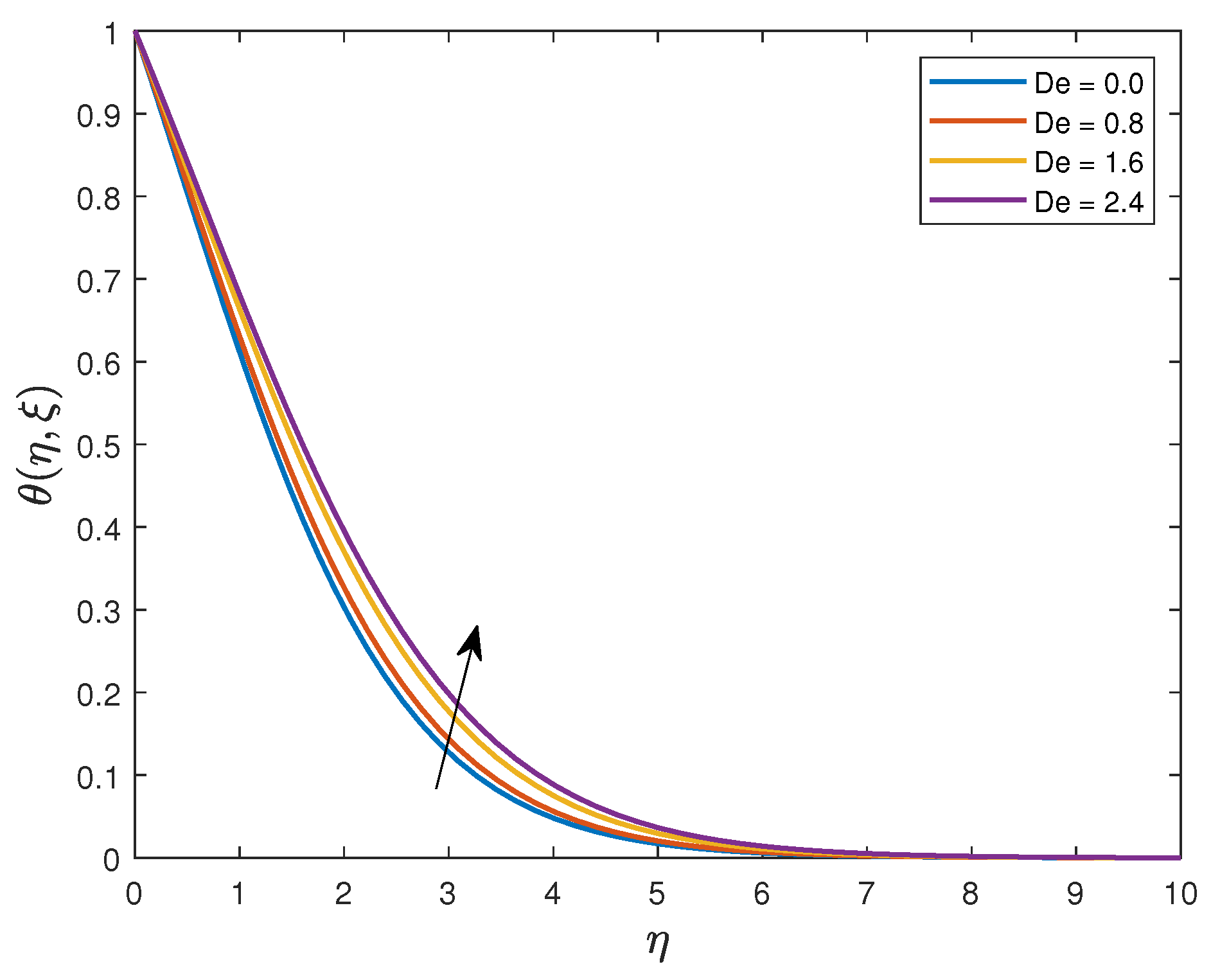
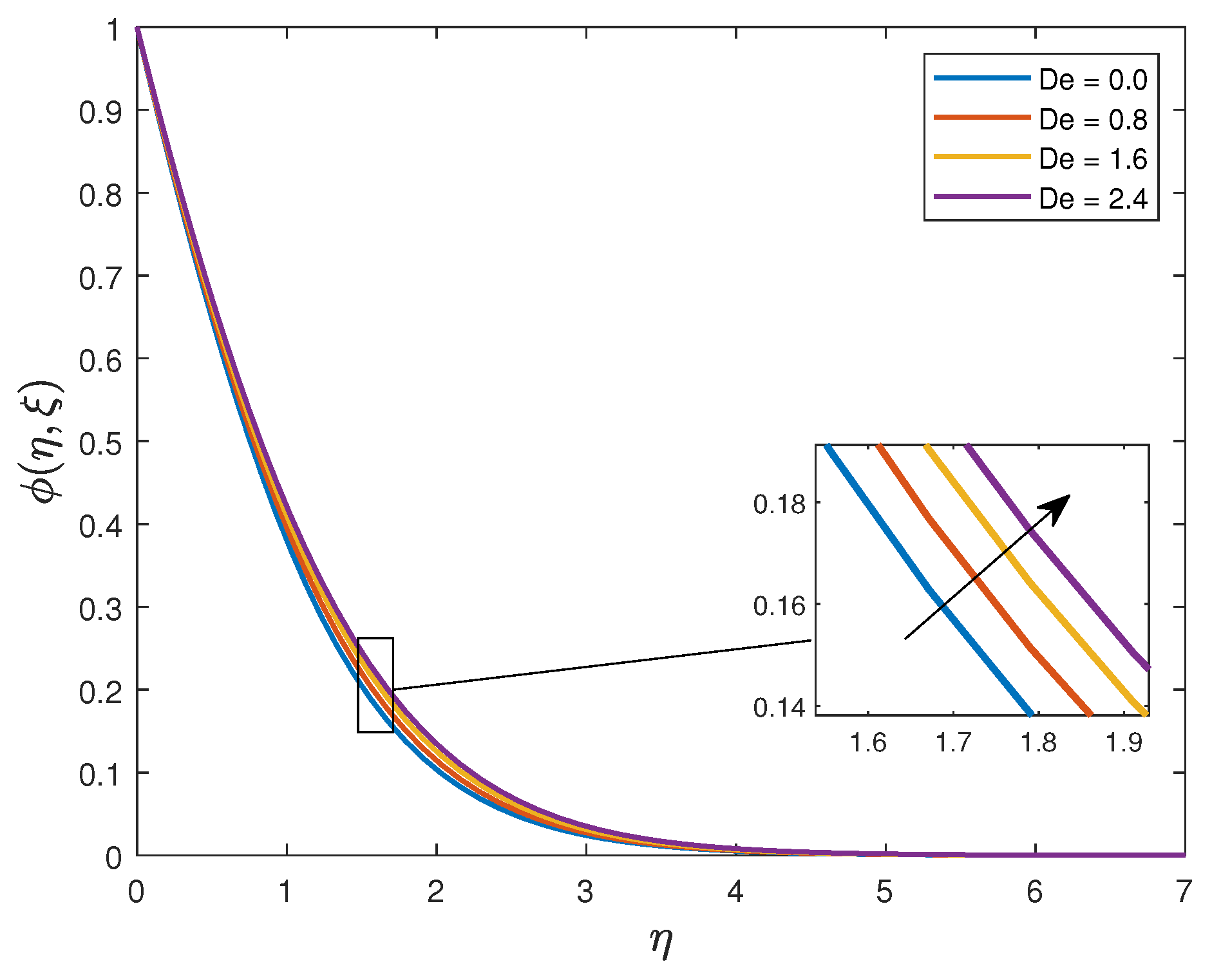
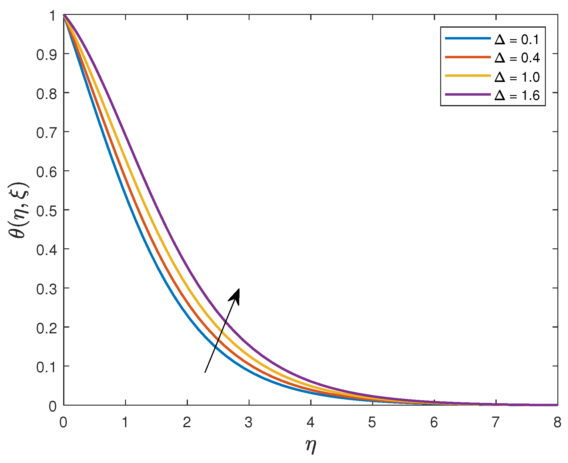
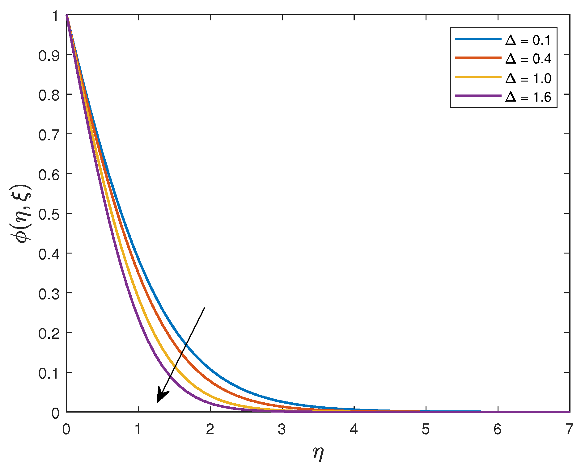
The variation of the fluid velocity, temperature, and concentration with increasing Schmidt number is illustrated in Figure 10, Figure 11 and Figure 12. The dimensionless Schmidt number relates the momentum diffusivity to mass diffusivity. The concentration of the fluid is decreased with the enhanced values of . A decrease in the concentration has an effect of suppressing the concentration buoyancy effects which, in turn, will reduce the fluid velocity. However, the opposite trend is realised for the fluid temperature. Figure 13, Figure 14 and Figure 15 reflect the effects of increasing the Deborah number on the fluid velocity, temperature and concentration profiles, respectively. The importance of the Deborah number in rheology is to define the fluidity of any material under the given specific conditions. A fluid becomes more solid-like with increasing values of the Deborah number, hence a significant decrease in the fluid velocity profile near the vertical plate. For both the fluid temperature and concentration, a similar behaviour is observed when the Deborah number is increased. It is also noted that in the concentration boundary layer, the Deborah number has an insignificant effect on the fluid far away from the vertical plate.
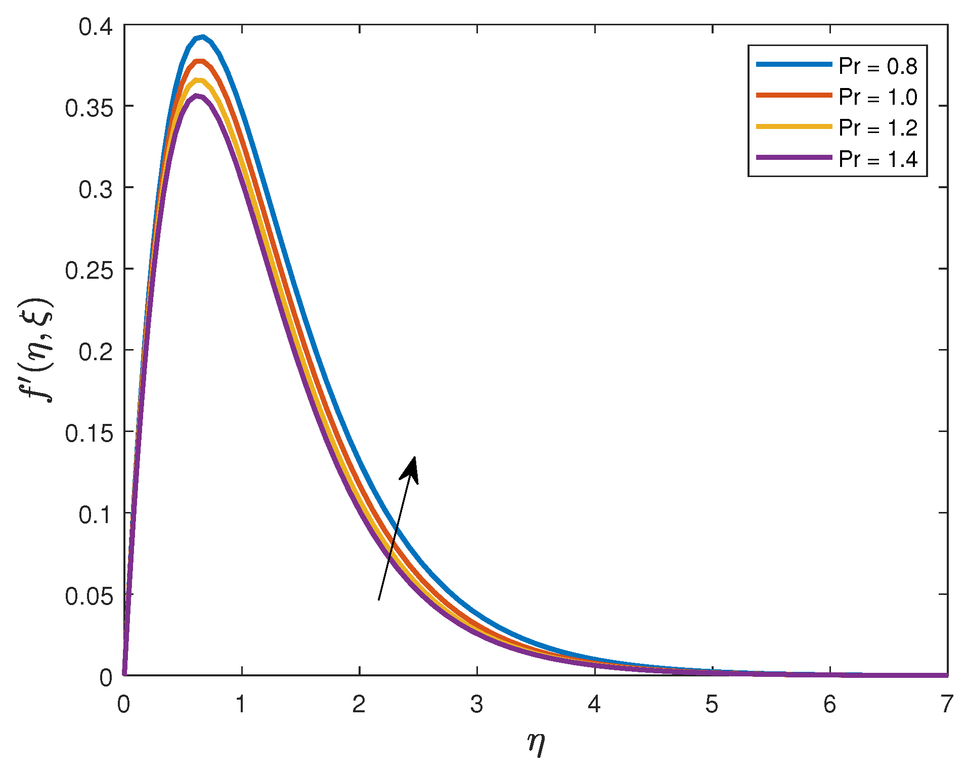
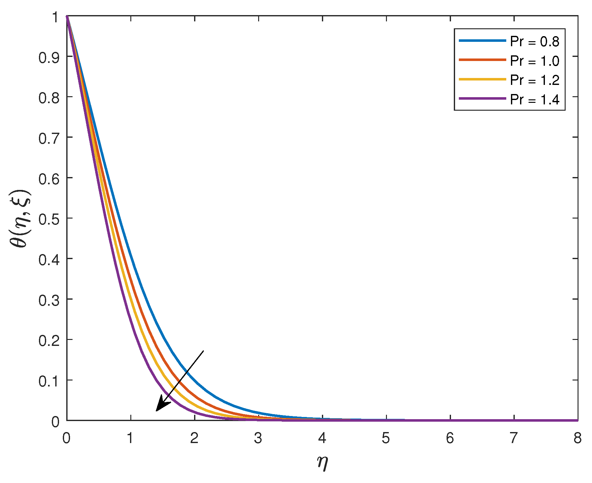
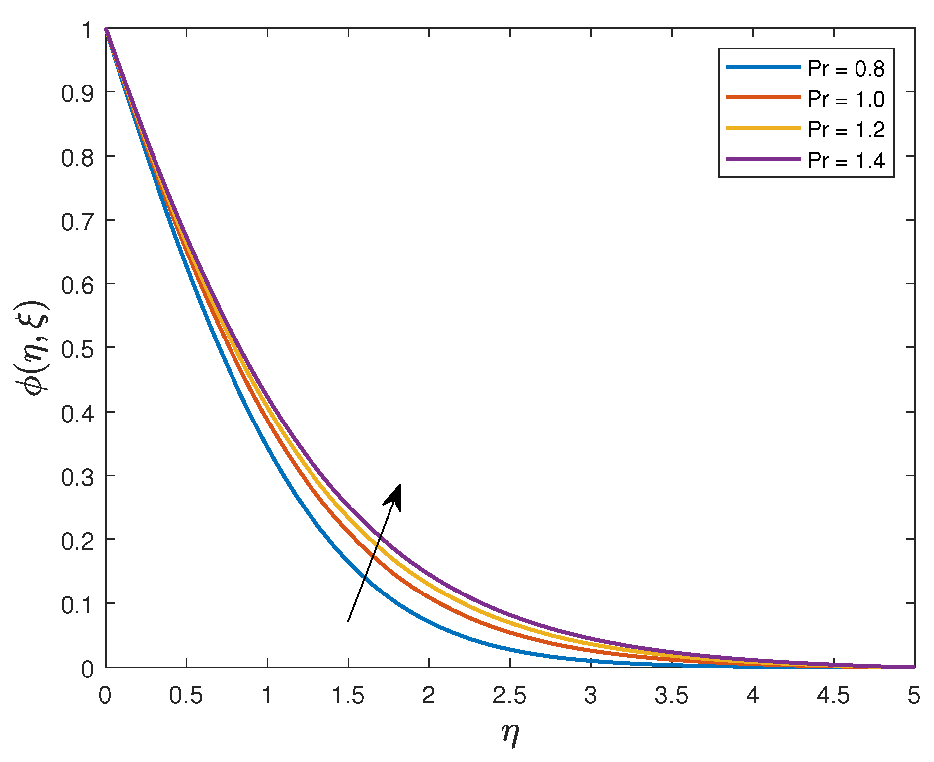
The effects of increasing the Prandtl number on the velocity, temperature, and concentration profiles of the Jeffrey fluid are illustrated in Figure 16, Figure 17 and Figure 18. It is observed that both the fluid velocity and temperature are depressed as increases whilst the concentration is enhanced. The Prandtl number approximates the ratio of the momentum diffusion to thermal diffusion. Increasing the values is equivalent to decreasing thermal diffusion. This will result in the thinning of the thermal boundary layer and hence reduced fluid temperature. Figure 19, Figure 20 and Figure 21 present the influence of the chemical reaction parameter on the fluid velocity, temperature, and concentration profiles, respectively. With increasing , the fluid velocity slightly decreases near the vertical plate and also slightly increase far away from the plate. Increasing the chemical reaction parameter has an effect of reducing the fluid solute concentration. Physically, increasing results in a reduced concentration boundary layer due to reduced species concentration.
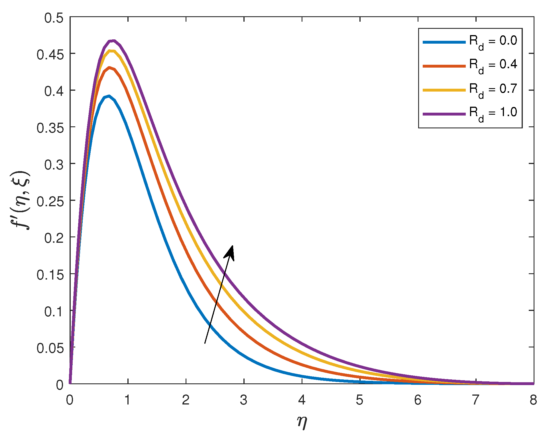
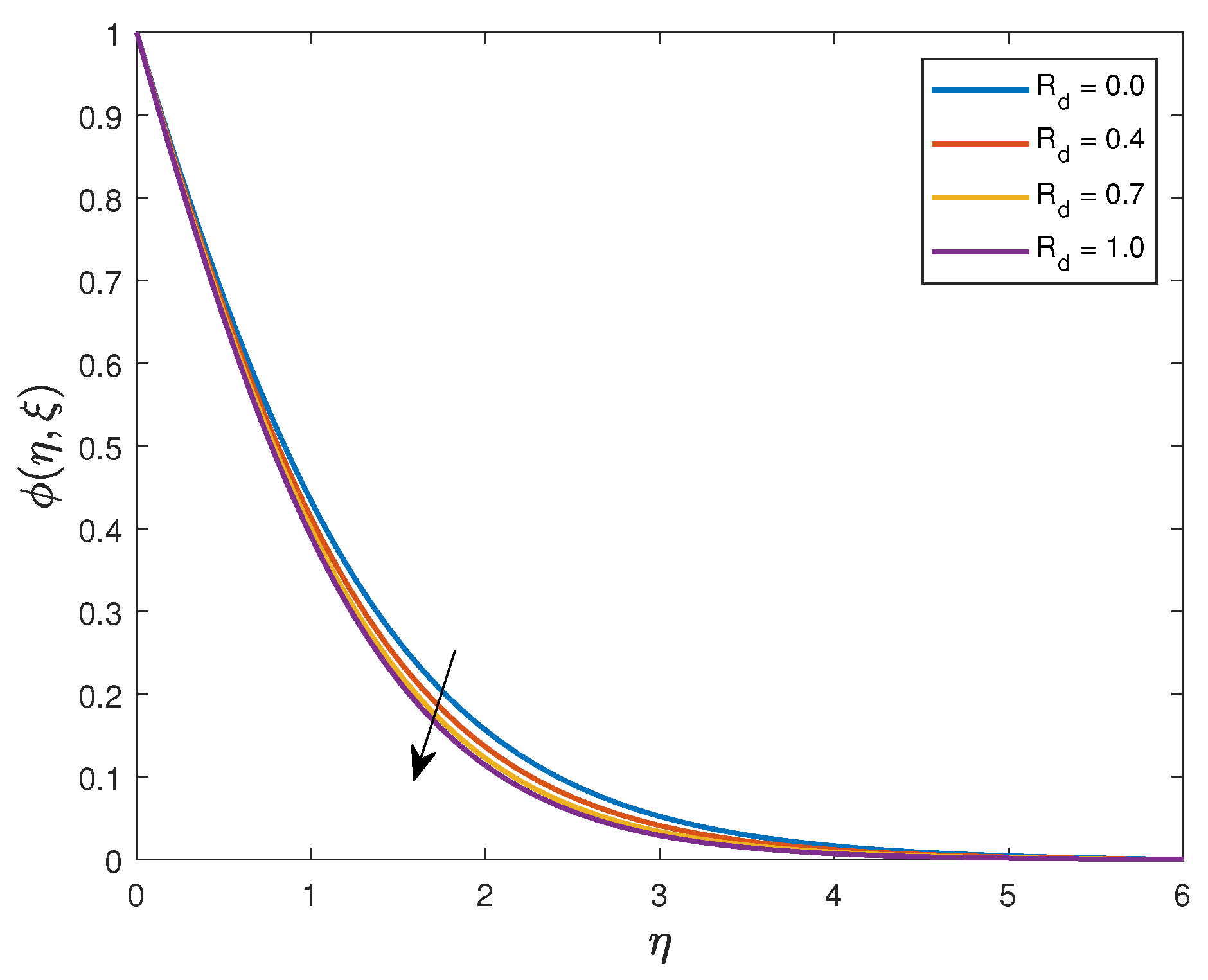
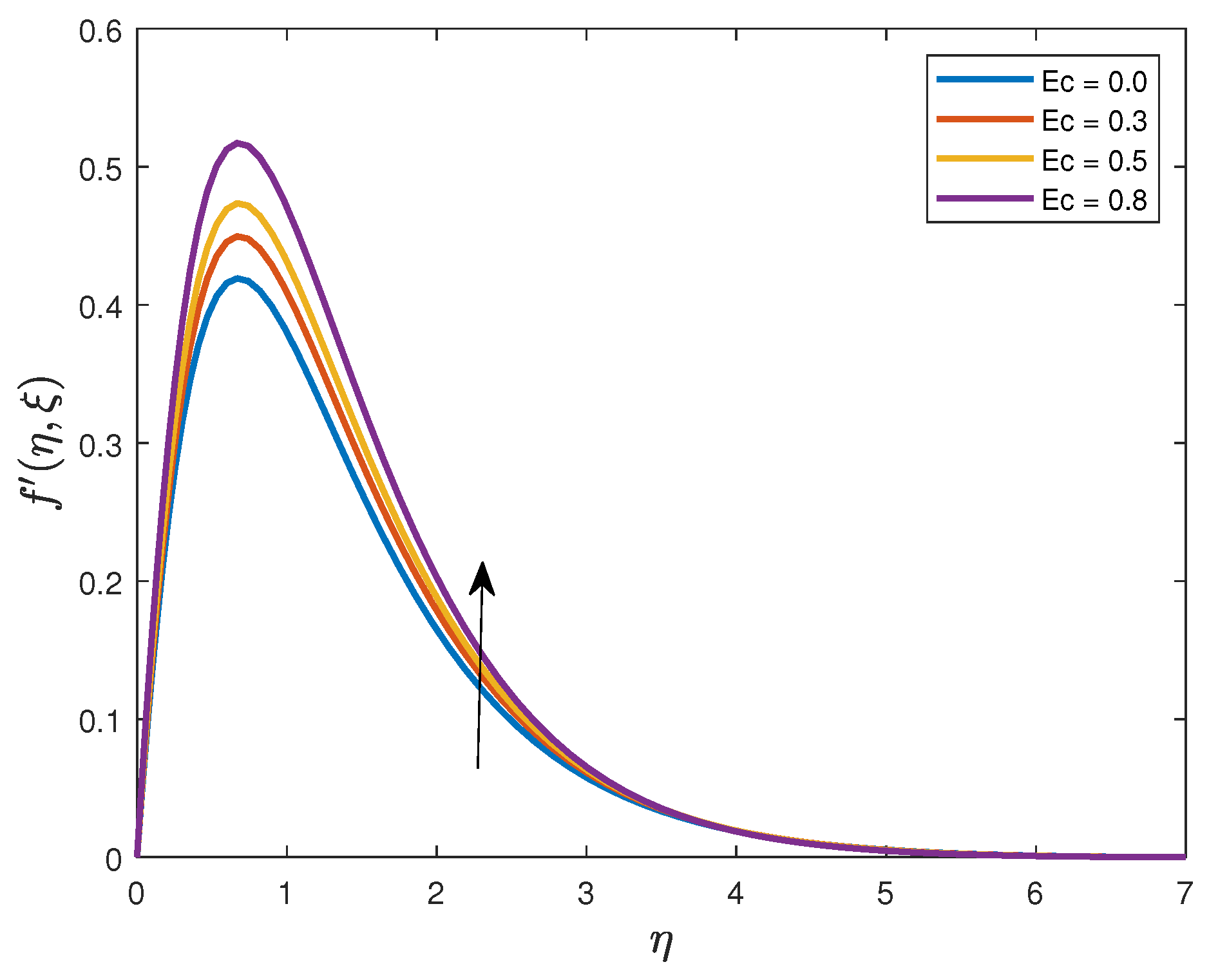
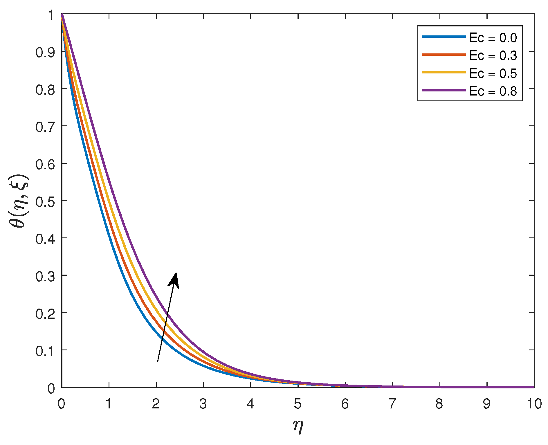
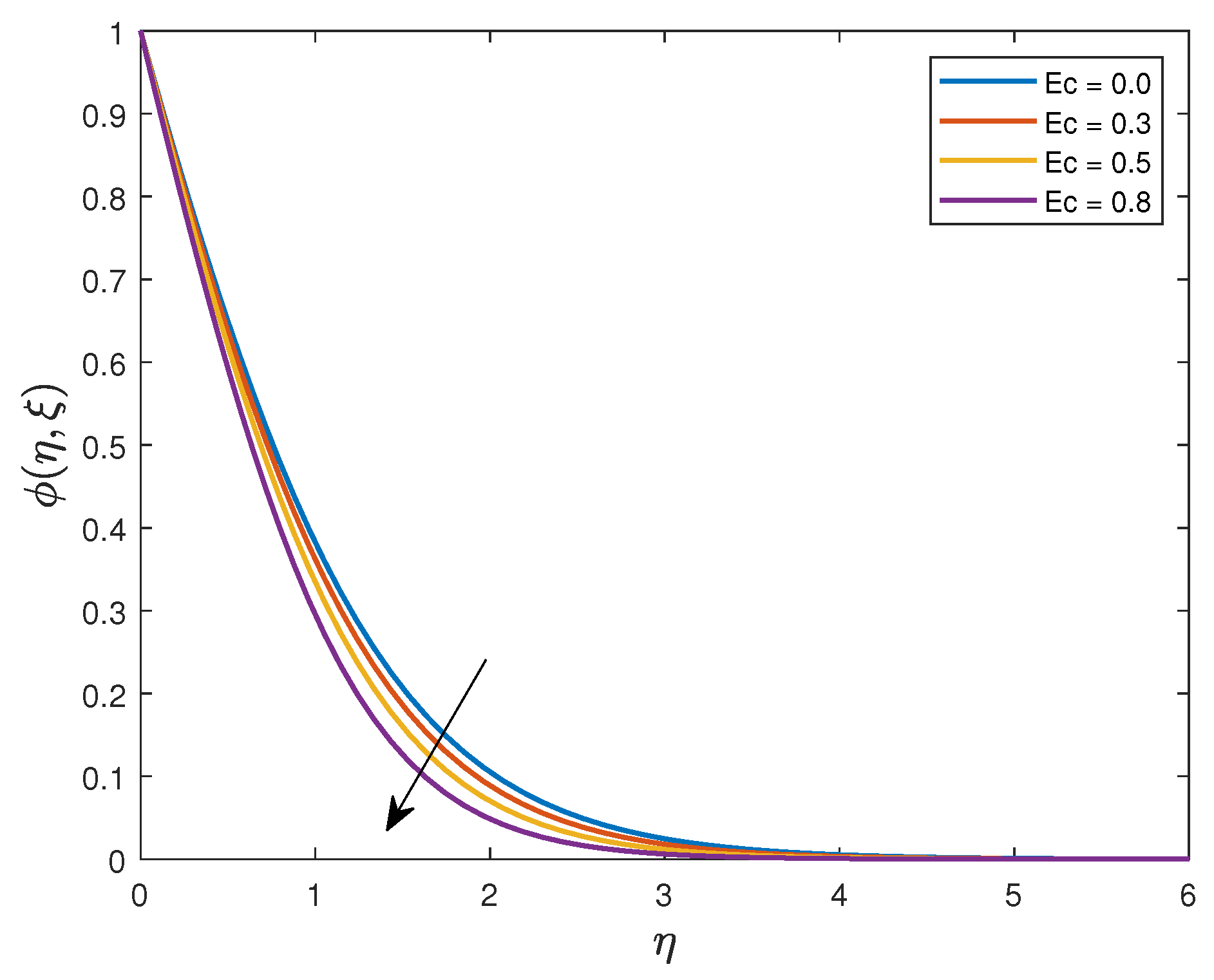
Figure 22, Figure 23 and Figure 24 show that the fluid velocity and temperature profiles are enhanced by an increase in the thermal radiation parameter, , whilst the concentration is depressed. Physically, increasing the thermal radiation parameter means more heat is emitted by the Jeffrey fluid causing a rise in the temperature and thickening of the thermal boundary layer. The Eckert number is a dimensionless number that provides a measure of the effects of self-heating of a fluid due to dissipation effects. From Figure 25, Figure 26 and Figure 27, it can be seen that an increasing values enhances velocity and temperature profiles. An opposite trend is observed in the case of the fluid concentration. Physically, increased values of the means more energy dissipating in the thermal boundary layer and this will cause an increase in the fluid temperature.
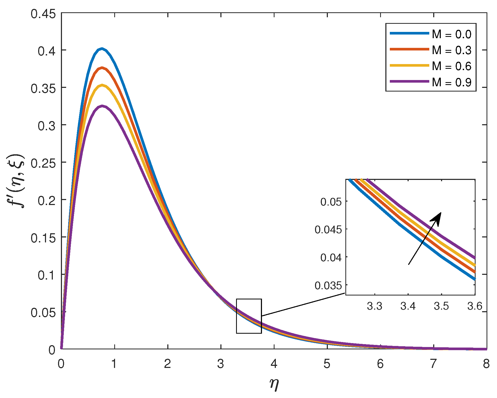
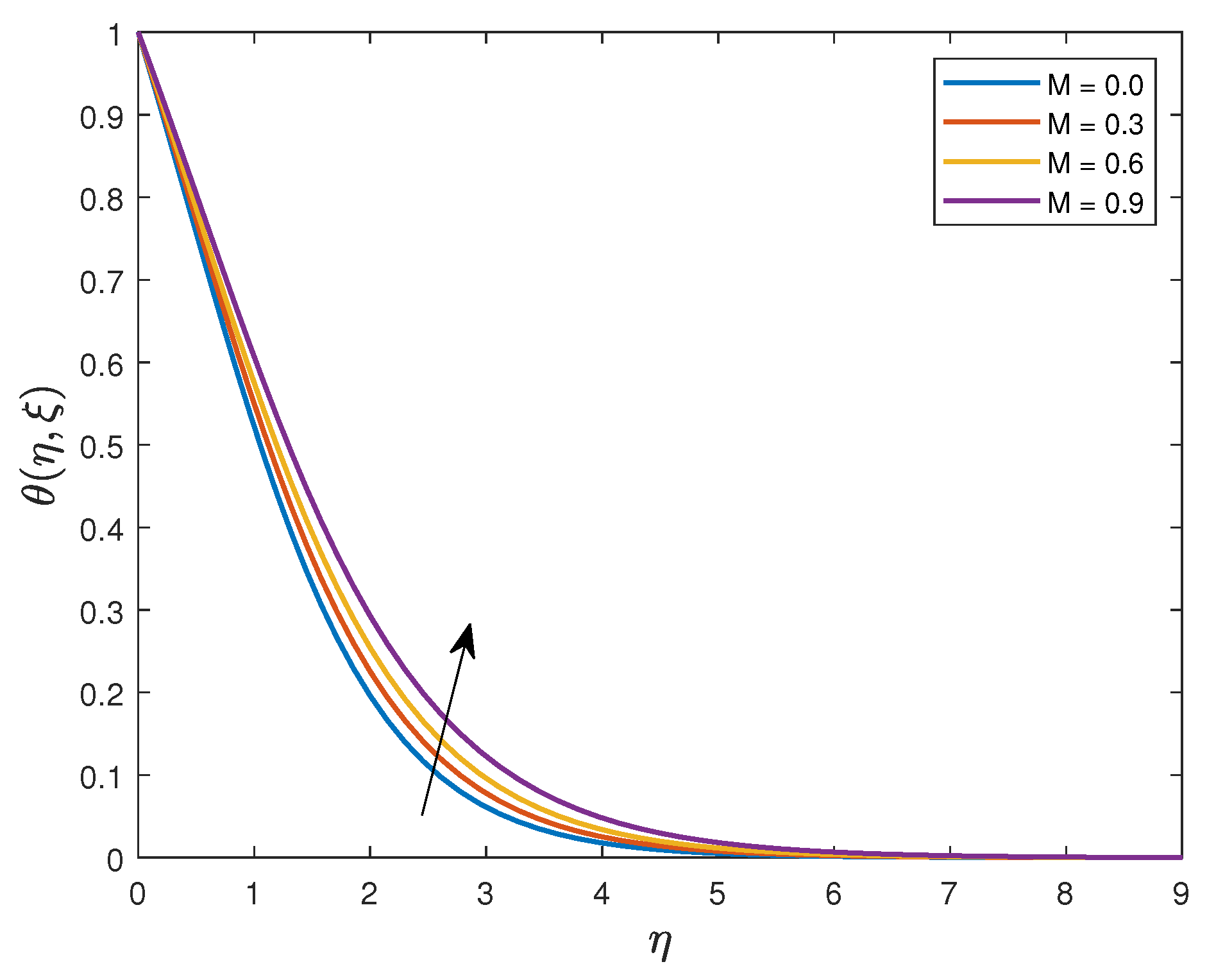
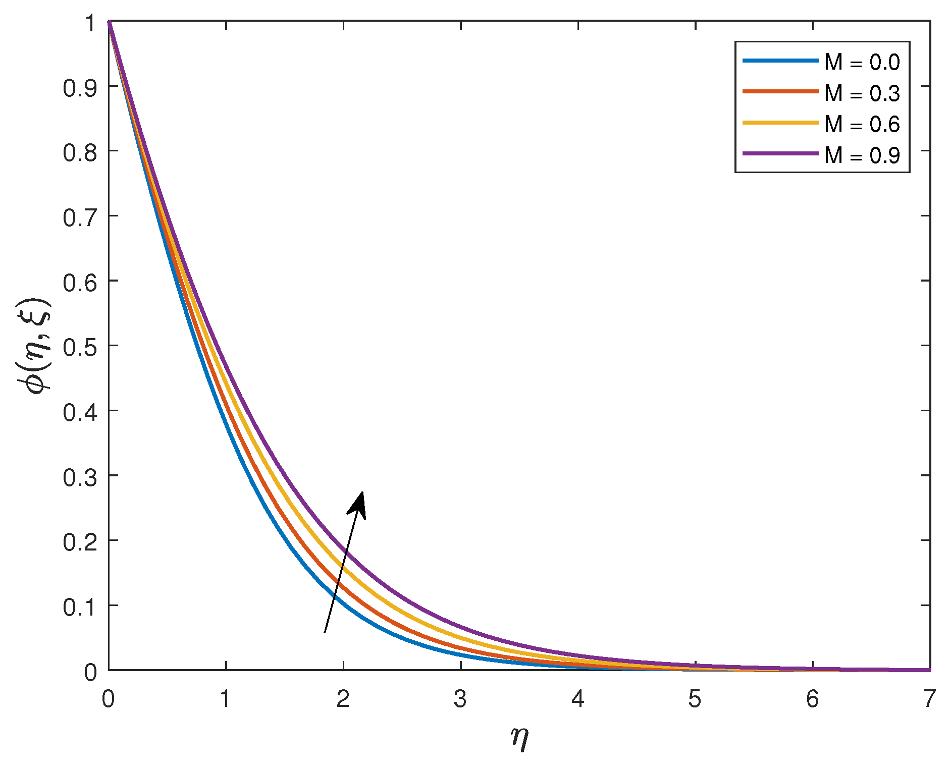
Figure 28, Figure 29 and Figure 30 depict the variations of the fluid velocity, temperature, and concentration with the magnetic field parameter, M. It is shown that the velocity of the fluid decreases with increasing values of M whilst both the temperature and concentration profiles are enhanced. The velocity and the momentum boundary layer of the fluid are reduced due to the resistive Lorentz force which tends to oppose the fluid flow. The presence of the heat source is seen to cause an increase in the fluid velocity and temperature, as shown in Figure 31 and Figure 32. However, it is revealed in Figure 33 that the concentration profile is suppressed as the values of are increased. Increasing heat source generates some heat in the thermal boundary layer thickness and the temperature distribution is also increased.
Table 1 displays the variation of the skin friction coefficient, local Nusselt number and the local Sherwood number for various values of the embedded parameters, namely , , , , M, and . It is noted that both the skin friction coefficient and the local Sherwood number are depressed with increasing values of , whilst the Nusselt number is increased. When is increased, it means the thermal boundary layer will be thinner relative to the momentum boundary layer. This will result in a large temperature difference and hence an increase in the heat transfer rate. An increase in the Schmidt number causes a decrease in the skin friction coefficient and the Nusselt number whilst the Sherwood number is increased. Increasing the Schmidt number has the effect of decreasing the molecular diffusion and hence a higher concentration of the species. We observe that increasing the values of increases the skin friction coefficient, local Nusselt number and the local Sherwood number. From Table 1 we can infer that increasing the values of the Deborah number reduces the skin friction coefficient, Nusselt number and Sherwood number. Physically, increasing means the fluid elasticity is increased whilst the the viscosity is reduced, as well as the frictional force on the plate. We can see that the values of the skin friction coefficient, local Nusselt number, and the local Sherwood number diminish as the values of M are increased. Increasing the Eckert number enhances the skin friction coefficient and the Sherwood number whilst the local Nusselt number is reduced.
5. Conclusions
In this current study, a numerical investigation of the magneto-hydrodynamic laminar boundary flow of a Jeffrey fluid past a vertical plate influenced by viscous dissipation and a heat source or sink was completed. Suitable similarity transformations were used to transform the governing partial differential equations into dimensionless differential equations which were then solved using the bivariate spectral quasi-linearisation method. Some of the most significant findings from this study are the following:
- The bivariate spectral quasi-linearisation method is a very accurate and efficient numerical technique for solving non-linear differential problems;
- Increasing the values of the concentration to thermal buoyancy ratio, radiation parameter, Eckert number, and the heat generation parameter will result in the enhancement of both the fluid velocity and the momentum boundary layer. The opposite trend is observed when the values of the ratio of relaxation to retardation times, Schmidt number, Deborah number, Prandtl number, chemical reaction parameter, and magnetic field parameter are increased;
- The fluid temperature increases with increasing values of the Schmidt number, Deborah number, chemical reaction parameter, radiation parameter, Eckert number, magnetic field parameter, and heat generation parameter, whilst it is reduced with an increase in the values of the ratio of relaxation to retardation times, concentration to thermal buoyancy ratio, and the Prandtl number;
- The fluid concentration is an increasing function of Deborah number, Prandtl number, and the magnetic field parameter whilst decreasing with respect to ratio of relaxation to retardation times, concentration to thermal buoyancy ratio, Schmidt number, chemical reaction parameter, radiation parameter, Eckert number, and the heat generation parameter;
- The local skin friction coefficient is observed to increase with increasing values of the ratio of relaxation to retardation times and the Eckert number. However, it diminishes with increasing values of the Prandtl number, Schmidt number, Deborah number, and magnetic field parameter;
- Increasing the Prandtl number and the ratio of relaxation to retardation times tend to increase the heat transfer rate whilst a decrease is observed when the Schmidt number, Deborah number, magnetic field parameter, and the Eckert number are increased;
- Lastly, the current study observed that the local Sherwood number increase when Schmidt number, the ratio of relaxation to retardation times and the Eckert number are increased whilst it is reduced with increasing Prandtl number, Deborah number, and the magnetic fiels parameter.
Author Contributions
Methodology, H.M. and S.S.; formal analysis, H.M. and S.S.; investigation, H.M. and S.S.; data curation, H.M. and S.S.; writing—original draft preparation, H.M. and S.S. All authors have read and agreed to the published version of the manuscript.
Funding
This research was funded by the University of Venda through funding my research visit, as well as the publication charges.
Institutional Review Board Statement
Not applicable.
Informed Consent Statement
Not applicable.
Data Availability Statement
Not applicable.
Acknowledgments
The assistance from the honourable editor and the anonymous reviewers in the preparation of this article is highly acknowledged.
Conflicts of Interest
The authors declare no conflict of interest. The funders had no role in the design of the study; in the collection, analyses, or interpretation of data; in the writing of the manuscript, or in the decision to publish the results.
References
- Cioranescu, D.; Girault, V.; Rajagopal, K.R. Mechanics and Mathematics of Fluids of the Differential Type. Adv. Mech. Math. 2016, 35, 1. [Google Scholar] [CrossRef]
- Nazeer, M.; Hussain, F.; Ahmad, M.O.; Saeed, S.; Khan, M.I.; Kadry, S.; Chu, Y.-M. Multi-phase flow of Jeffrey Fluid bounded within Magnetized Horizontal Surface. Surf. Interfaces 2020, 100846. [Google Scholar] [CrossRef]
- Nadeem, S.; Akhtar, S.; Saleem, A. Peristaltic flow of a heated Jeffrey fluid inside an elliptic duct: Streamline analysis. Appl. Math. Mech. Engl. Ed. 2021, 42, 583–592. [Google Scholar] [CrossRef]
- Fetecau, C.; Ellahi, R.; Sait, S.M. Mathematical Analysis of Maxwell Fluid Flow through a Porous Plate Channel induced by a Constantly Accelerating or Oscillating Wall. Mathematics 2021, 9, 90. [Google Scholar] [CrossRef]
- Sajid, M.; Jagwal, M.R.; Ahmad, I. Numerical and perturbative analysis on non-axisymmetric Homann stagnation-point flow of Maxwell fluid. SN Appl. Sci. 2021, 3, 438. [Google Scholar] [CrossRef]
- Elhanafy, A.; Guaily, A.; Elsaid, A. Numerical simulation of Oldroyd-B fluid with application to hemodynamics. Adv. Mech. Eng. 2019, 11, 168781401985284. [Google Scholar] [CrossRef] [Green Version]
- Wang, J.; Khan, M.I.; Khan, W.A.; Abbas, S.Z.; Khan, M.I. Transportation of heat generation/absorption and radiative heat flux in homogeneous-heterogeneous catalytic reactions of non-Newtonian fluid (Oldroyd-B model). Comput. Methods Programs Biomed. 2019, 105310. [Google Scholar] [CrossRef]
- Priyadharshini, S.; Ponalagusamy, R. Biorheological Model on Flow of Herschel-Bulkley Fluid through a Tapered Arterial Stenosis with Dilatation. Appl. Bionics Biomech. 2015, 1–12. [Google Scholar] [CrossRef]
- Magnon, E.; Cayeux, E. Precise Method to Estimate the Herschel-Bulkley Parameters from Pipe Rheometer Measurements. Fluids 2021, 6, 157. [Google Scholar] [CrossRef]
- Kahshan, M.; Lu, D.; Siddiqui, A.M. A Jeffrey Fluid Model for a Porous-walled Channel: Application to Flat Plate Dialyzer. Sci. Rep. 2019, 9. [Google Scholar] [CrossRef] [Green Version]
- Akbar, N.S.; Nadeem, S.; Lee, C. Characteristics of Jeffrey fluid model for peristaltic flow of chyme in small intestine with magnetic field. Results Phys. 2013, 3, 152–160. [Google Scholar] [CrossRef] [Green Version]
- Sharma, B.D.; Yadav, P.K.; Filippov, A. A Jeffrey-fluid model of blood flow in tubes with stenosis. Colloid J. 2017, 79, 849–856. [Google Scholar] [CrossRef]
- Nallapu, S.; Radhakrishnamacharya, G. Jeffrey Fluid Flow through Porous Medium in the Presence of Magnetic Field in Narrow Tubes. Int. J. Eng. Math. 2014, 1–8. [Google Scholar] [CrossRef] [Green Version]
- Ellahi, R.; Rahman, S.U.; Nadeem, S. Blood flow of Jeffrey fluid in a catherized tapered artery with the suspension of nanoparticles. Phys. Lett. A 2014, 378, 2973–2980. [Google Scholar] [CrossRef]
- Khan, A.; Zaman, G.; Algahtani, O. Unsteady Magnetohydrodynamic Flow of Jeffrey Fluid through a Porous Oscillating Rectangular Duct. Porosity Process. Technol. Appl. 2018, 125–128. [Google Scholar] [CrossRef] [Green Version]
- Vaidya, H.; Rajashekhar, C.; Divya, B.B.; Manjunatha, G.; Prasad, K.V.; Animasaun, I.L. Influence of transport properties on the peristaltic MHD Jeffrey fluid flow through a porous asymmetric tapered channel. Results Phys. 2020, 18, 103295. [Google Scholar] [CrossRef]
- Ahmad, K.; Ishak, A. Magnetohydrodynamic (MHD) Jeffrey fluid over a stretching vertical surface in a porous medium. Propuls. Power Res. 2017, 6, 269–276. [Google Scholar] [CrossRef]
- Nadeem, S.; Zaheer, S.; Fang, T. Effects of thermal radiation on the boundary layer flow of a Jeffrey fluid over an exponentially stretching surface. Numer. Algorithms 2010, 57, 187–205. [Google Scholar] [CrossRef]
- Hayat, T.; Asad, S.; Qasim, M.; Hendi, A.A. Boundary layer flow of a Jeffrey fluid with convective boundary conditions. Int. J. Numer. Methods Fluids 2011, 69, 1350–1362. [Google Scholar] [CrossRef]
- Tlili, I. Effects MHD and Heat Generation on Mixed Convection Flow of Jeffrey Fluid in Microgravity Environment over an Inclined Stretching Sheet. Symmetry 2019, 11, 438. [Google Scholar] [CrossRef] [Green Version]
- Babu, D.; Venkateswarlu, S.; Keshava Reddy, E. Multivariate Jeffrey Fluid Flow past a Vertical Plate through Porous Medium. J. Appl. Comput. Mech. 2020, 6, 605–616. [Google Scholar] [CrossRef]
- Selvi, R.K.; Muthuraj, R. MHD oscillatory flow of a Jeffrey fluid in a vertical porous channel with viscous dissipation. Ain Shams Eng. J. 2017, 9, 2503–2516. [Google Scholar] [CrossRef]
- Amanulla, C.H.; Nagendra, N.; Surya Narayana Reddy, M.; Subba Rao, A.; Sudhakar Reddy, M. Heat Transfer in a Non-Newtonian Jeffery Fluid from an Inclined Vertical Plate. Indian J. Sci. Technol. 2017, 10, 1–5. [Google Scholar] [CrossRef] [Green Version]
- Prasad, V.R.; Gaffar, S.A.; Reddy, E.K.; Bég, O.A. Numerical Study of Non-Newtonian Boundary Layer Flow of Jeffreys Fluid Past a Vertical Porous Plate in a Non-Darcy Porous Medium. Int. J. Comput. Methods Eng. Sci. Mech. 2014, 15, 372–389. [Google Scholar] [CrossRef]
- Hayat, T.; Shehzad, S.A.; Qasim, M.; Obaidat, S. Radiative flow of Jeffery fluid in a porous medium with power law heat flux and heat source. Nucl. Eng. Des. 2012, 243, 15–19. [Google Scholar] [CrossRef]
- Nisar, K.S.; Mohapatra, R.; Mishra, S.R.; Reddy, M.G. Semi-analytical solution of MHD of free convective Jeffrey fluid flow in the presence of heat source and chemical reaction. Ain Shams Eng. J. 2020, 12, 837–845. [Google Scholar] [CrossRef]
- Hussain, Z.; Hussain, A.; Anwar, M.S.; Farooq, M. Analysis of Cattaneo–Christov heat flux in Jeffery fluid flow with heat source over a stretching cylinder. J. Therm. Anal. Calorim. 2021. [Google Scholar] [CrossRef]
- Qasim, M. Heat and mass transfer in a Jeffrey fluid over a stretching sheet with heat source/sink. Alex. Eng. J. 2013, 52, 571–575. [Google Scholar] [CrossRef] [Green Version]
- Motsa, S.S.; Magagula, V.M.; Sibanda, P. A Bivariate Chebyshev Spectral Collocation Quasilinearization Method for Nonlinear Evolution Parabolic Equations. Sci. World J. 2014, 1–13. [Google Scholar] [CrossRef] [Green Version]
- Magagula, V.M.; Motsa, S.S.; Sibanda, P. On the bivariate spectral quasilinearization method for nonlinear boundary layer partial differential equations. Appl. Heat Mass Fluid Bound. Layers 2020, 177–190. [Google Scholar] [CrossRef]
- Rai, N.; Mondal, S. Spectral methods to solve nonlinear problems: A review. Partial Diff. Eqn. Appl. Math. 2021, 4, 100043. [Google Scholar]
- Goqo, S.P.; Oloniiju, S.D.; Mondal, H.; Sibanda, P.; Motsa, S.S. Entropy generation in MHD radiative viscous nanofluid flow over a porous wedge using the bivariate spectral quasi-linearization method. Case Stud. Therm. Eng. 2018. [Google Scholar] [CrossRef]
- Motsa, S.S.; Ansari, M.S. Unsteady boundary layer flow and heat transfer of Oldroyd-B nanofluid towards a stretching sheet with variable thermal conductivity. Therm. Sci. 2015, 19, S239–S248. [Google Scholar] [CrossRef]
- Ijaz, M.; Ayub, M. Thermally stratified flow of Jeffrey fluid with homogeneous-heterogeneous reactions and non-Fourier heat flux model. Heliyon 2019, 5, e02303. [Google Scholar] [CrossRef] [PubMed] [Green Version]
- Khan, I. A Note on Exact Solutions for the Unsteady Free Convection Flow of a Jeffrey Fluid. Z. FüR Naturforschung A 2015, 70. [Google Scholar] [CrossRef]
- Abdul Gaffar, S.; Ramachandra Prasad, V.; Keshava Reddy, E. Computational study of Jeffrey’s non-Newtonian fluid past a semi-infinite vertical plate with thermal radiation and heat generation/absorption. Ain Shams Eng. J. 2017, 8, 277–294. [Google Scholar] [CrossRef] [Green Version]
- El-Aziz, M.A.; Yahya, A.S. Heat and Mass Transfer of Unsteady Hydromagnetic Free Convection Flow Through Porous Medium Past a Vertical Plate with Uniform Surface Heat Flux. J. Theor. Appl. Mech. 2017, 47, 25–58. [Google Scholar] [CrossRef] [Green Version]
- Alharbey, R.A.; Mondal, H.; Behl, R. Spectral Quasi-Linearization Method for Non-Darcy Porous Medium with Convective Boundary Condition. Entropy 2019, 21, 838. [Google Scholar] [CrossRef] [Green Version]
- Trefethen, L.N. Spectral Methods in MATLAB; Society for Industrial and Applied Mathematics: Philadelphia, PA, USA, 2000; pp. 51–59. [Google Scholar]
Figure 1.
Schematic flow diagram and coordinate system.

Figure 2.
Convergence graphs of , , and .

Figure 3.
Accuracy graphs of , , and .

Figure 4.
The influence of on fluid velocity.

Figure 5.
The influence of on fluid temperature.

Figure 6.
The influence of on fluid concentration.

Figure 7.
The influence of K on fluid velocity.

Figure 8.
The influence of K on fluid temperature.

Figure 9.
The influence of K on fluid concentration.

Figure 10.
The influence of on fluid velocity.

Figure 11.
The influence of on fluid temperature.

Figure 12.
The influence of on fluid concentration.

Figure 13.
The influence of on fluid velocity.

Figure 14.
The influence of on fluid temperature.

Figure 15.
The influence of on fluid concentration.

Figure 16.
The influence of on fluid velocity.

Figure 17.
The influence of on fluid temperature.

Figure 18.
The influence of on fluid concentration.

Figure 19.
The influence of on fluid velocity.

Figure 20.
The influence of on fluid temperature.

Figure 21.
The influence of on fluid concentration.

Figure 22.
The influence of on fluid velocity.

Figure 23.
The influence of on fluid temperature.

Figure 24.
The influence of on fluid concentration.

Figure 25.
The influence of on fluid velocity.

Figure 26.
The influence of on fluid temperature.

Figure 27.
The influence of on fluid concentration.

Figure 28.
The influence of M on fluid velocity.

Figure 29.
The influence of M on fluid temperature.

Figure 30.
The influence of M on fluid concnetration.

Figure 31.
The influence of on fluid velocity.

Figure 32.
The influence of on fluid temperature.

Figure 33.
The influence of on fluid concentration.


Table 1.
Computed values of the skin friction coefficient, local Nusselt number and local Sherwood number for different values of , , , M and when , , , , .
Table 1.
Computed values of the skin friction coefficient, local Nusselt number and local Sherwood number for different values of , , , M and when , , , , .
| M | ||||||||
|---|---|---|---|---|---|---|---|---|
| 0.1 | 0.6 | 0.2 | 0.1 | 0.5 | 0.1 | 1.030290 | 0.266186 | 2.080584 |
| 0.2 | 0.841704 | 0.434430 | 2.055455 | |||||
| 0.3 | 0.705153 | 0.600888 | 2.036738 | |||||
| 0.4 | 0.601525 | 0.767872 | 2.022356 | |||||
| 0.1 | 0.6 | 0.2 | 0.1 | 0.5 | 0.1 | 1.030290 | 0.266186 | 2.080584 |
| 1.0 | 1.023224 | 0.266066 | 3.277721 | |||||
| 1.4 | 1.019745 | 0.266026 | 4.468999 | |||||
| 1.8 | 1.017726 | 0.266008 | 5.659950 | |||||
| 0.1 | 0.6 | 0.2 | 0.1 | 0.5 | 0.1 | 1.030290 | 0.266186 | 2.080584 |
| 0.8 | 1.333454 | 0.268194 | 2.095147 | |||||
| 1.4 | 1.594027 | 0.269306 | 2.104991 | |||||
| 2.0 | 1.826278 | 0.270002 | 2.112276 | |||||
| 0.1 | 0.6 | 0.2 | 0.1 | 0.5 | 0.1 | 1.030290 | 0.266186 | 2.080584 |
| 0.3 | 0.708783 | 0.261353 | 2.058275 | |||||
| 0.5 | 0.577533 | 0.258195 | 2.046650 | |||||
| 0.7 | 0.500040 | 0.255768 | 2.038835 | |||||
| 0.1 | 0.6 | 0.2 | 0.1 | 0.5 | 0.1 | 1.030290 | 0.266186 | 2.080584 |
| 1.0 | 0.920258 | 0.259580 | 2.068256 | |||||
| 1.5 | 0.828255 | 0.253782 | 2.057571 | |||||
| 2.0 | 0.751381 | 0.248726 | 2.048362 | |||||
| 0.1 | 0.6 | 0.2 | 0.1 | 0.5 | 0.1 | 1.030290 | 0.266186 | 2.080584 |
| 0.5 | 1.032627 | 0.260233 | 2.080870 | |||||
| 0.9 | 1.034988 | 0.254216 | 2.081158 | |||||
| 1.3 | 1.037374 | 0.248135 | 2.081449 |
Publisher’s Note: MDPI stays neutral with regard to jurisdictional claims in published maps and institutional affiliations. |
© 2021 by the authors. Licensee MDPI, Basel, Switzerland. This article is an open access article distributed under the terms and conditions of the Creative Commons Attribution (CC BY) license (https://creativecommons.org/licenses/by/4.0/).
Share and Cite
MDPI and ACS Style
Muzara, H.; Shateyi, S. MHD Laminar Boundary Layer Flow of a Jeffrey Fluid Past a Vertical Plate Influenced by Viscous Dissipation and a Heat Source/Sink. Mathematics 2021, 9, 1896. https://doi.org/10.3390/math9161896
AMA Style
Muzara H, Shateyi S. MHD Laminar Boundary Layer Flow of a Jeffrey Fluid Past a Vertical Plate Influenced by Viscous Dissipation and a Heat Source/Sink. Mathematics. 2021; 9(16):1896. https://doi.org/10.3390/math9161896
Chicago/Turabian StyleMuzara, Hillary, and Stanford Shateyi. 2021. "MHD Laminar Boundary Layer Flow of a Jeffrey Fluid Past a Vertical Plate Influenced by Viscous Dissipation and a Heat Source/Sink" Mathematics 9, no. 16: 1896. https://doi.org/10.3390/math9161896
Note that from the first issue of 2016, this journal uses article numbers instead of page numbers. See further details here.