Integral Equations Related to Volterra Series and Inverse Problems: Elements of Theory and Applications in Heat Power Engineering

Abstract

The paper considers two types of Volterra integral equations of the first kind, arising in the study of inverse problems of the dynamics of controlled heat power systems. The main focus of the work is aimed at studying the specifics of the classes of Volterra equations of the first kind that arise when describing nonlinear dynamics using the apparatus of Volterra integro-power series. The subject area of the research is represented by a simulation model of a heat exchange unit element, which describes the change in enthalpy with arbitrary changes in fluid flow and heat supply. The numerical results of solving the problem of identification of transient characteristics are presented. They illustrate the fundamental importance of practical recommendations based on sufficient conditions for the solvability of linear multidimensional Volterra equations of the first kind. A new class of nonlinear systems of integro-algebraic equations of the first kind, related to the problem of automatic control of technical objects with vector inputs and outputs, is distinguished. For such systems, sufficient conditions are given for the existence of a unique, sufficiently smooth solution. A review of the literature on these problem types is given.

1. Introduction

Present power plants belong to the category of complex technical systems, the study of the functioning dynamics of which is based on the formalization of the physical nature of the object (obtaining an analytical model), on carrying out natural experiments (using a real model), as well as on the use of simulation models that describe processes in actual time. In terms of content, the models for controlling the modes of power plants are of the adaptive type. The classification of control objects for energy systems and energy units is given in [1]. Depending on the formulation of the control criterion, the following areas of research can be conditionally singled out:

(1)

Problems with statistical or dynamic technological criteria (optimization of the basic parameters of the boiler unit [2], temperature control [3], maximum efficiency of combustion processes [4,5], changes in design parameters [6], etc.);

(2)

Problems with statistical or dynamic technical and economic criteria (energy-saving of thermal energy [7], minimization of operating costs [8], maximum profit [9], etc.);

(3)

Forecasting problems for the technical state of heat and power equipment (short-term and long-term forecasts of the mode parameters [10,11], planning of repair and maintenance work, development of a strategy for equipment service [12], etc.);

(4)

Multicriteria control problems, including emergency control from the point of view of reliability [13], optimization of technical indicators of energy sources depending on their location [14], a hybrid approach for correcting a certain combination of various characteristics [15], and so forth.

Traditionally, the methodology for controlling the modes of power systems has taken into account the principles of hierarchical modeling. As a rule, the lower level of the control system structural diagram contains automated control systems for the dynamics of local devices. Analysis of scientific and technical literature shows that the development of mathematical tools for the study of such devices remains an important production task. As noted in [16], intelligent approaches based on the application of the theory of fuzzy sets [17] and artificial neural networks [18] are quite promising for the optimization of technological indicators.

In this paper, we consider a technique based on the Volterra functional series [19] for constructing integral models, the transient characteristics (Volterra kernels) of which change in the time domain. Note this mathematical apparatus is used in practice both independently [20] and in combination with the theory of neural networks [21] to approximate the nonlinear dynamics of “input–output”-type objects. In addition, the difference analog of Volterra polynomials (finite segments of the series) is the basis for the creation of one of the types of neural networks [22,23]. Numerical methods and algorithms for the computer implementation of such models, due to the versatility of the Volterra series theory, have proven themselves well in problems with the identification and modeling of the basic parameters of various technical objects of heat and power engineering.

In particular, based on the data of a physical experiment carried out on the high-temperature circuit (HTC) of the Melentiev Energy Systems Institute, a simulation model for describing the dynamics of an electrically heated pipeline section is constructed in the form of a quadratic Volterra polynomial [24]. A similar research area is considered in [25], wherein the monitoring of heat exchange processes in the M-1 EP-300 condenser of the Angarsk Polymer Plant is realized using an integral model. Integral models are successfully used to analyze the dynamics of electro-mechanical devices, for example, to simulate the angular speed of the rotation of blades of a wind generator [26], as well as to diagnose the current state of a reluctance motor [27]. The simulation model, formed using the technique [28] from the diagonal values of the kernels of the cubic Volterra polynomial, makes it possible to control the value of the air gap between the rotor and the stator of the electric motor without object-taking out of service. The dynamics of a laminator with a DC motor is studied in [29]. The approximating model, formed using the Volterra and Laguerre polynomials of the first order, is used to analyze the relationship between the parameters of the technological process: voltage, current, and clamping speed during double-sided lamination.

Thus, the development of mathematical modeling methods based on the theory of the Volterra series and their applications in power engineering is relevant not only from a scientific, but also from a practical point of view. Obviously, these methods should be focused on solving a whole spectrum of problems, including the study of new classes of integral equations (IE) of the Volterra type, the study of the properties of numerical methods for their solution, as well as the substantiation of practical recommendations that ensure the effective implementation of computational algorithms. The focus is on the specifics of the two classes of Volterra equations of the first kind arising in the solution of inverse problems of nonlinear dynamics, in the description of which the theory of Volterra integro-power series is used. The effectiveness of solving these problems is illustrated in the paper on a simulation model of a radiation heat exchanger, which is considered below as a “reference” model. The description of the subject area and the heuristic rationale for the choice of the modeling quality indicator is given in Section 2.

The purpose of the paper is to present the solution to inverse problems that play an important role in the theory of automatic control [30] and are associated with the creation of a unified approach to modeling dynamic systems of the “input–output” type using Volterra polynomials:

$$y(t)=P_N(x(t))={\displaystyle \sum _{m = 1}^N{\displaystyle \sum _{1 \le i_1 \le \dots \le i_m \le p}{V}_{i_1 \dots i_m}(x(t))}},$$

(1)

$$V_{i_1 \dots i_m}(x(t))={\displaystyle \underset{0}{\overset{t}{\int }}\dots {\displaystyle \underset{0}{\overset{t}{\int }}{K}_{i_1 \dots i_m}(t,s_1,\dots ,s_m){\displaystyle \prod _{l = 1}^m{x}_{i_l}(s_l)d{s}_l}}}, t\in [0,T],$$

(2)

where the input signal $x(t)={(x_1(t),\dots ,x_p(t))}^T$ and the output $y(t)$ are functions of time $t$. In Equation (2), the functions $K_{i_1\dots i_n}(t,s_1,\dots ,s_m)$ are called Volterra kernels, which, in the terminology of [31], are invariant under the replacement of $s_j$ by $s_k$ under $i_j=i_k$.

Selected types of inverse problems are devoted to:

-

Identification of the transient characteristics of the dynamic system (Section 3);

-

Identification of the input signals of the dynamic system (Section 4).

Some facts from the theory of multidimensional linear integral equations with variable limits of integration and their application to the problem of identifying transient characteristics are described in Section 3.1 and Section 3.2, respectively. Section 4 is devoted to the results of the study of Volterra polynomial integral equations related to the problem of automatic control of technical objects with vector inputs. Additionally, Section 4 addresses the further development of the work.

2. Description of the Subject Area

The subject area of the paper is presented by nonlinear dynamic systems, for which the following is true:

• The system is not a developing one (according to the terminology of [32]), only dynamic connections of the “input–output” type are taken into account;
• The connection between the input $x(t)$ and output $y(t)$ is unidirectional, that is, the response of the system does not have an indirect effect on the input;
• The system is in a steady state at the initial time, that is, the output signal remains unchanged at a constant input action, while we assume $x(t_0)=0$, $y(t_0)=0$, $t_0=0$);
• It is allowed to carry out an active experiment that assumes the possibility of influencing the dynamic system with test input signals of the step type with the constant height (amplitude). In addition, external control of the input actions is allowed.

The change in enthalpy $\Delta i(t)$ with arbitrary changes in the flow rate of liquid $\Delta D(t)$ and heat supply $\Delta Q(t)$ in the radiation element of the heat exchanger was chosen as a simulation model obtained in [33] under the assumption of a linear variation of the parameters to the spatial variable:

$$\Delta i(t)=\frac{{\lambda }_1{\lambda }_2}{{\lambda }_2-{\lambda }_1}{\displaystyle \underset{0}{\overset{t}{\int }}\left(\Delta Q(\eta )-\frac{Q_0}{D_0}\Delta D(\eta )\right)\left(e^{-{\lambda }_1{\displaystyle \underset{\eta }{\overset{t}{\int }}D(\xi )d\xi }}-e^{-{\lambda }_2{\displaystyle \underset{\eta }{\overset{t}{\int }}D(\xi )d\xi }}\right)d\eta },$$

(3)

where $D(t)=\Delta D(t)+D_0$, ${\lambda }_1$, ${\lambda }_2$ are the roots of the characteristic equation for a system of two first-order differential equations. The initial values for the calculations were $D_0=0.16$ (kg/s), $Q_0=100$ (kW), $i_0=1059$ (kJ/kg), time $t\in [0,T]$. In the context of Equation (3), $x(t)={(x_1(t),x_2(t))}^T$ and $y(t)$ from Equations (1) and (2) under $p=2$ are defined as follows: $x_1(t)\equiv \Delta D(t)$, $x_2(t)\equiv \Delta Q(t)$, $y(t)\equiv \Delta i(t)$. Herewith, in accordance with item iii, $\Delta D(0)=0$, $\Delta Q(0)=0$, $\Delta i(0)=0$. The value for the right boundary of the time range $T=30$ (s) was selected based on the results of calculations according to Equation (3). It was found that under input actions $\Delta D(t)$, $\Delta Q(t)$ of a stepwise form, the response $\Delta i(t)$ of a dynamic system is stabilized ($\Delta i(t)=\mathrm{const}$ for $t\ge t_k$) with an accuracy of $\delta ={10}^{-1}$ for $t_k\ge 30$ (s). Model Equation (3) describes the dynamics $\Delta i(t)$ of an element of a heat exchanger with a single-phase incompressible fluid in which a substance flow moves during external heating. Note that when studying the dynamics of the enthalpy of complex apparatuses, as a rule, a longer time range is considered, for example, $T=3000$ s in [34].

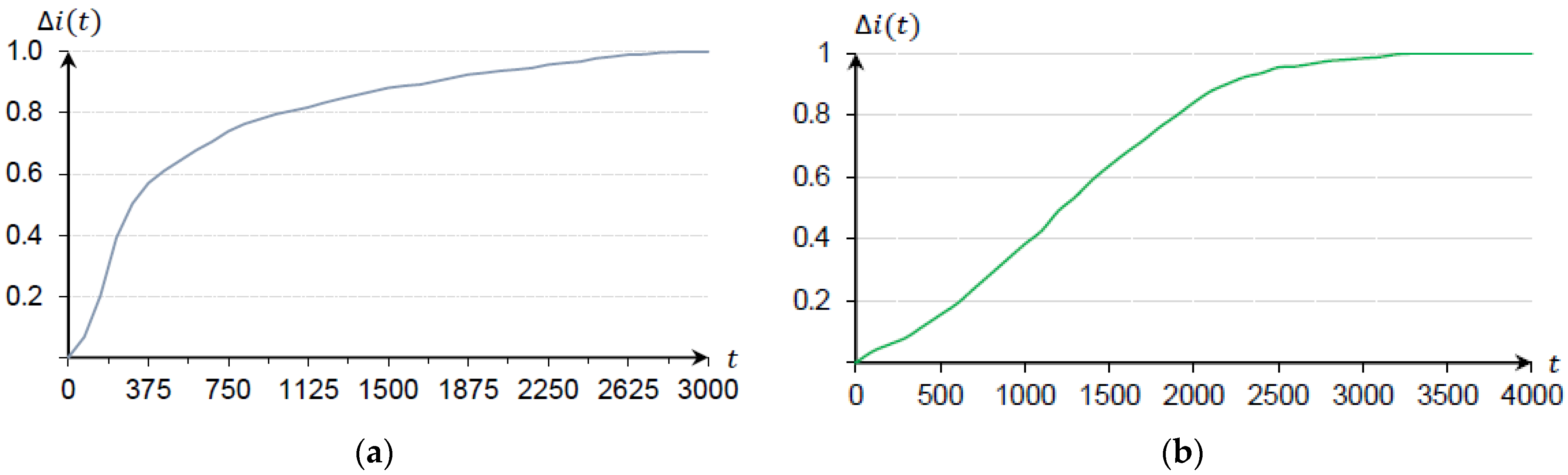
Nevertheless, the simulation model Equation (3) is important from a methodological point of view for comparative analysis of the accuracy of numerical methods and verification of computational algorithms. A normalized graph of the change in the enthalpy of steams at the outlet of the direct-flow boiler TGMP-314P in the mode of 70% of the nominal load with disturbance of the feed water flow rate for $T=3000$ s was obtained in work [34] (p. 35) (see Figure 1a). Using a distributed parameter model, the values $\Delta i(t)$ at the outlet of the boiler unit economizer with a deep change in the coolant flow rate for $T=4000$ s were calculated in [35]. Figure 1b shows the normalized graph.

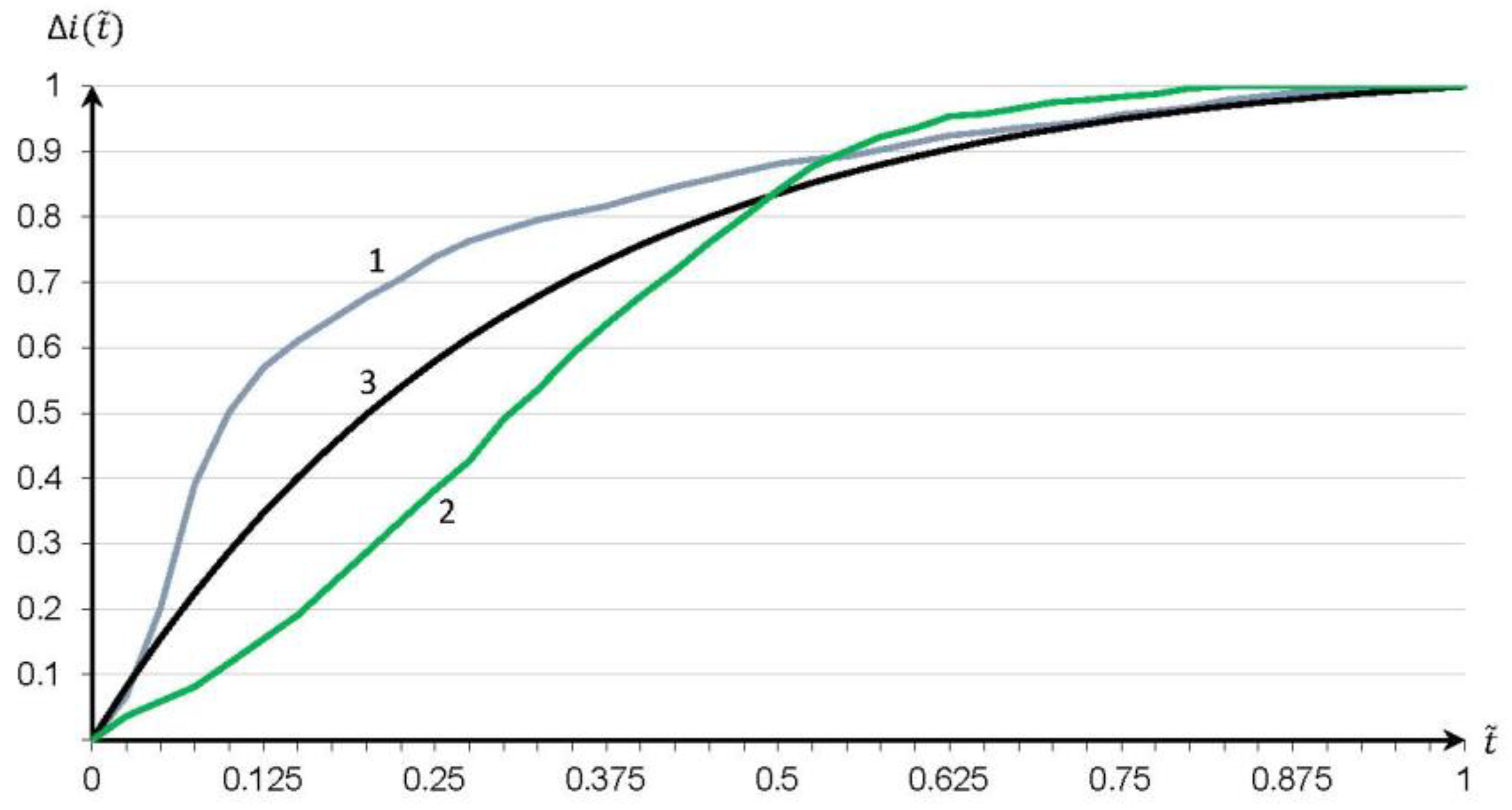
Figure 2 compares the graphs of the dependences $\Delta i(\tilde{t})$ at dimensionless time $\tilde{t}=\frac{t}{T}$, obtained with single precision calculations using various models: the direct-flow boiler (graph 1), the boiler unit economizer (graph 2), and the single heat exchanger (3) (at $\Delta Q(t)=0$, $\Delta D(t)=0.25\cdot D_0$) (graph 3). Calculations have shown that at $\tilde{t}\in [0.9,1]$, normalized values of all three functions coincide within $\delta ={10}^{-3}$. Thus, practical recommendations for using the apparatus of the Volterra series, obtained to model Equation (3), can be applied to study the dynamics of complex heat-and-power objects.

Thus, based on the analysis of the normalized graphs shown in Figure 2, as a criterion for the accuracy of modeling, we select the modulus of deviation of the model $y(t)$ response in the form of the Volterra polynomial Equations (1) and (2) from the values of $\Delta i(t)$ according to Equation (3) at the end of the transient process at $t=T$. Note that at the stage of computational experiments, the following assumptions were made in the work:

-

At the input $x(t)$ and output $y(t)$ of the dynamic system, deviations from those indicators that are observed in the steady state are considered;

-

The values of input $x(t)$ and output $y(t)$ can be measured at fixed times;

-

The responses of the dynamical system $y(t)$ for $t\in [0,T]$ have sufficient smoothness.

The simulation model Equation (3) was used to develop specific recommendations for choosing an approximating Volterra polynomial. These recommendations include conditions on the amplitudes $\alpha$ of test signals. It should be noted that the developed recommendations were successfully tested both for the integral model of transient processes of heat power objects [24] and for the test mathematical model [36].

3. The Problem of Identifying Transient Characteristics

3.1. Volterra Equations of the First Kind with Two Variable Integration Limits

To construct an integral model of the form Equation (1), it is required to solve the problem of nonparametric identification of Volterra kernels (transient characteristics of a dynamic system) in Equation (2). The practical application of such models in the time domain is still limited [20]. As the analysis of the scientific and technical literature has shown, when describing dynamic systems corresponding to the selected subject area, an approach based on the use of test inputs in the form of Heaviside functions:

$$e(t)=\{\begin{array}{ll}0,\hspace{0.17em}\hspace{0.17em}\hfill & t\le 0,\hfill \\ 1,\hspace{0.17em}\hspace{0.17em}\hspace{0.17em}\hfill & t>0,\hfill \end{array}$$

is quite common. A shortlist of publications on the use of learning sample signals of this type is shown in the review of [36]. It should be noted that as a rule (see, for example, [37]), researchers turn to the consideration of discrete analogs of Equations (1) and (2), that is, to the problem of solving some system of linear algebraic equations (SLAE), leaving beyond the scope of theoretical research directly multidimensional integral equations. On the one hand, this reduction allows one to obtain a difference approximation of the desired solution. As shown in the thesis [38] (pp. 298–299), the mesh analogs of integral equations, due to the nondegeneracy of the corresponding SLAEs, are uniquely solvable for any right-hand side. On the other hand, a qualitative study of the corresponding classes of multidimensional integral equations helps to remove the arbitrariness in the choice of specific parameters of test signals and to obtain practical recommendations at the stage of preparation for conducting experiments. Indeed, as shown in [36,39], the choice of the amplitude of the test signals in the identification of Volterra kernels $K_{i_1 \dots i_n}$, $N>2$, is associated with the necessary conditions for the solvability of the corresponding multidimensional integral equations in special classes of functions.

Thus, the specificity of the Volterra integral equations related to the problem of identifying transient characteristics is fundamentally important for the effective implementation of the developed numerical methods in practice. This section is devoted to multidimensional linear Volterra equations of the first kind arising in the construction problem, Equation (1),

$$V_{i_1 \dots i_m}(x(t))={\displaystyle \underset{0}{\overset{t}{\int }}\dots {\displaystyle \underset{0}{\overset{t}{\int }}{K}_{i_1\dots i_m}(s_1,\dots ,s_m){\displaystyle \prod _{l = 1}^m{x}_{i_l}(t-s_l)d{s}_l}}}, t\in [0,T],$$

(4)

based on piecewise constant functions with deviating argument [40]

$$x_{{\omega }_1,\dots ,\hspace{0.17em}{\omega }_{m-1}}^{\alpha }(t)=\alpha \left[e(t)+2{\displaystyle \sum _{k=1}^{m-2}{(-1)}^{k}e\left(t-{\displaystyle \sum _{i=1}^k{\omega }_i}\right)+{(-1)}^{m-1}e\left(t-{\displaystyle \sum _{i=1}^{m-1}{\omega }_i}\right)}\right],$$

(5)

$0\le t,\hspace{0.17em}\hspace{0.17em}{\omega }_i\le T,\hspace{0.17em}$ $i=\overline{1,m-1},\hspace{0.17em}$ $\hspace{0.17em}m\ge 2$. Note that signals $x_{{\omega }_1, \dots , {\omega }_{m-1}}^{\alpha }$ of the form (5) are included in the feasible set of input signals of the physical system (see item iv of Section 2). The application of test signals Equation (5), where $\alpha$ is an amplitude, and ${\omega }_1,\dots ,{\omega }_{m-1}$ are durations of the input action, allows us to reduce the original problem of identifying kernels in Equation (4) to the solution of a multidimensional Volterra integral equation of the first kind with variable limits of integration under $0\le {\displaystyle \sum _{k = 1}^{m - 1}{\omega }_k\le t\le T,\hspace{0.17em}}{\omega }_k\ge 0$ that have the explicit inversion formulas [40]. Here, relation Equation (4) follows from Equation (2) under the assumption that the dynamical system is stationary (i.e., the Volterra kernels $K_{i_1 \dots i_m}$ depend on the difference $t-s_j$, $j=\overline{1,m}$). The situation when a dynamical system is nonstationary was considered in [41].

The technique of using scalar input signals in Equation (5) is described in detail in the review [42] (see the section “About one approach to identification of Volterra kernels”). For the case of a signal represented as a vector function of time, the series of articles [36,39,42,43,44] presents algorithms for choosing the amplitudes of test signals for identifying Volterra kernels, which, in general, can be represented as follows:

• Empirical stage. Analysis of a priori information about an object to select the type of integral model and a method for setting responses $y(t)$ to test signals of a step type.
• Implementation of the decomposition algorithm, taking into account the necessary conditions for the solvability of the corresponding integral equations in the required class of functions [36,39]. The decomposition algorithm was considered in the case when the analytical form of output signals is known for scalar test input signals [41].
• Experimental debugging. Determination of the optimal values of the amplitudes based on the solution of some extremal problems introduced in [42,43].

The results presented in [42] on the identifying Volterra kernels in integral models Equations (1) and (3) for the scalar case $\hspace{0.17em}x(t)\equiv x_i(t)$, $\hspace{0.17em}N=2$

$$\hspace{0.17em}{y}_2(t)={\displaystyle \underset{0}{\overset{t}{\int }}{K}_i(s)x(t-s)}ds+{\displaystyle \underset{0}{\overset{t}{\int }}{\displaystyle \underset{0}{\overset{t}{\int }}{K}_{ii}}}(s_1,s_2)x(t-s_1)x(t-s_2)d{s}_{1}d{s}_2,$$

(6)

and $\hspace{0.17em}N=3$

$$\begin{array}{cc}\hspace{0.17em}{y}_3(t)& ={\displaystyle \underset{0}{\overset{t}{\int }}{K}_i(s)x(t-s)}ds+{\displaystyle \underset{0}{\overset{t}{\int }}{\displaystyle \underset{0}{\overset{t}{\int }}{K}_{ii}}}(s_1,s_2)x(t-s_1)x(t-s_2)d{s}_{1}d{s}_2 +\hfill \\ & +{\displaystyle \underset{0}{\overset{t}{\int }}{\displaystyle \underset{0}{\overset{t}{\int }}{\displaystyle \underset{0}{\overset{t}{\int }}{K}_{iii}}}}(s_1,s_2,s_3)x(t-s_1)x(t-s_2)x(t-s_3)d{s}_{1}d{s}_{2}d{s}_3\hfill \end{array}$$

(7)

relied heavily on the symmetry property of $K_i$, $K_{ii}$, $K_{iii}$ concerning all arguments (it is a consequence of the assumption that the input signal is a scalar function of time). To identify the kernels $K_i$, $K_{ii}$, the input disturbances $x_{{\omega }_1}^{{\alpha }_{l,i}}(t)={\alpha }_{k,i}\left(e(t)-e(t-{\omega }_1)\right)$, $k=1,2$, $0\le {\omega }_1\le t\le T$ were used, the amplitudes ${\alpha }_{l,i}$ of which were selected based on condition

$${\alpha }_{1,i}+{\alpha }_{2,i}=0,$$

(8)

which follows from the belonging of the kernels $K_{ii}$ to the class of symmetric functions continuous on the square $0\le s_1, s_2\le T$. A similar condition [42]

$${\stackrel{⌢}{\alpha }}_{1,i}+{\stackrel{⌢}{\alpha }}_{2,i}+{\stackrel{⌢}{\alpha }}_{3,i}=0$$

(9)

for the amplitudes of test signals $x_{{\omega }_1}^{{\stackrel{⌢}{\alpha }}_{l,i}}(t)={\stackrel{⌢}{\alpha }}_{l,i}\left(e(t)-2e(t-{\omega }_1)+e(t-{\omega }_1-{\omega }_2)\right)$, $l=\overline{1,3}$, $0\le {\omega }_1+{\omega }_2\le t\le T$ follows from the necessary and sufficient conditions for the solvability of the three-dimensional Volterra integral equation of the first kind with variable upper and lower integration limits arising in the problem of identifying $K_{iii}$ from Equation (7). Let us further, for simplicity, present ${\alpha }_{1,i}=-{\alpha }_{2,i}\equiv {\alpha }_i$. As shown in [36], when selecting the amplitudes used to identify $K_i$ and $K_{ii}$ in (1), (4) for $\hspace{0.17em}N=3$, ${\alpha }_i$ requires coordination with the values ${\stackrel{⌢}{\alpha }}_{l,i}$, $l=\overline{1,3}$, such as

$${\alpha }_1^2=-\left({\stackrel{⌢}{\alpha }}_{1,i}\hspace{0.17em}{\stackrel{⌢}{\alpha }}_{2,i}+{\stackrel{⌢}{\alpha }}_{1,i}\hspace{0.17em}{\stackrel{⌢}{\alpha }}_{3,i}+{\stackrel{⌢}{\alpha }}_{2,i}\hspace{0.17em}{\stackrel{⌢}{\alpha }}_{3,i}\right).$$

(10)

In the case of vector input signals, in particular, for $x(t)={(x_1(t),x_2(t))}^T$, the right-hand side of Equation (1), in contrast to Equations (6) and (7), includes integral terms that take into account the contribution of nonsymmetric kernels $K_{12}$, $K_{112}$, and $K_{122}$. From the fulfillment of the conditions of the theorems on the existence of these kernels in the required classes of functions [36], constraints of the form

$${\beta }_{k,i}^2={\alpha }_{k,i}^2, {\gamma }_{k,i}^2={\alpha }_{k,i}^2$$

(11)

follow (test signals of the selected type with amplitudes ${\beta }_{k,1}$, ${\beta }_{k,2}$ are used to identify $K_{12}$, with amplitudes ${\gamma }_{k,1}$, ${\gamma }_{k,2}$—to identify $K_{112}$ and $K_{122}$).

It is interesting to analyze how violation of conditions Equations (8)–(11) at the stage of planning an experiment on a set of responses of a dynamic system, represented by a simulation model Equation (3), to inputs of the form Equation (5) will influence on the accuracy of constructing Equations (1) and (4) for $\hspace{0.17em}p=2$, $\hspace{0.17em}N = 2$

$$\begin{array}{c}\hspace{0.17em}{y}_2(t)={\displaystyle \sum _{i = 1}^2{\displaystyle \underset{0}{\overset{t}{\int }}{K}_i(s)x_i(t-s)}}ds+{\displaystyle \underset{0}{\overset{t}{\int }}{\displaystyle \underset{0}{\overset{t}{\int }}{K}_{11}}}(s_1,s_2)x_1(t-s_1)x_1(t-s_2)d{s}_{1}d{s}_2 +\\ +{\displaystyle \underset{0}{\overset{t}{\int }}{\displaystyle \underset{0}{\overset{t}{\int }}{K}_{12}}}(s_1,s_2)x_1(t-s_1)x_2(t-s_2)d{s}_{1}d{s}_2\end{array}$$

(12)

and $\hspace{0.17em}N=3$

$$\begin{array}{c}\hspace{0.17em}{y}_3(t)=\hspace{0.17em}{\displaystyle \sum _{i = 1}^2{\displaystyle \underset{0}{\overset{t}{\int }}{K}_i(s)x_i(t-s)}}ds+{\displaystyle \underset{0}{\overset{t}{\int }}{\displaystyle \underset{0}{\overset{t}{\int }}{K}_{11}}}(s_1,s_2)x_1(t-s_1)x_1(t-s_2)d{s}_{1}d{s}_2 +\\ +{\displaystyle \underset{0}{\overset{t}{\int }}{\displaystyle \underset{0}{\overset{t}{\int }}{K}_{12}}}(s_1,s_2)x_1(t-s_1)x_2(t-s_2)d{s}_{1}d{s}_2 +\\ +{\displaystyle \underset{0}{\overset{t}{\int }}{\displaystyle \underset{0}{\overset{t}{\int }}{\displaystyle \underset{0}{\overset{t}{\int }}{K}_{111}}}}(s_1,s_2,s_3)x_1(t-s_1)x_1(t-s_2)x_1(t-s_3)d{s}_{1}d{s}_{2}d{s}_3 +\\ +{\displaystyle \underset{0}{\overset{t}{\int }}{\displaystyle \underset{0}{\overset{t}{\int }}{\displaystyle \underset{0}{\overset{t}{\int }}{K}_{112}}}}(s_1,s_2,s_3)x_1(t-s_1)x_1(t-s_2)x_2(t-s_3)d{s}_{1}d{s}_{2}d{s}_3.\end{array}$$

(13)

Note that in Equations (12) and (13), under the linearity of Equation (3) concerning $\Delta Q(t)$, the kernels $K_{22}\equiv K_{122}\equiv K_{222}\equiv 0$. Further, we give the results of a computational experiment.

3.2. Computational Experiment Results

To obtain on a uniform mesh $t_i=ih$, $i=\overline{1,n}$, $h=\raisebox{1ex}{$T$}\!\left/ \!\raisebox{-1ex}{$n$}\right.\hspace{0.17em}$, the difference analogs of the responses of the simulation Equation (3) and integral models Equations (12) and (13), we will use the author’s software and computer complex [43]. We use the trapezoidal method to calculate the values $y_{et}(t_i)\equiv \Delta i(t_i)$ and the middle rectangles method to calculate the values $y_2(t_i)$, $y_3(t_i)$. As a criterion for the accuracy of modeling, we select the relative residual between $y_{et}(t)$ and $y_2(t)$, $y_3(t)$ at $t=T$:

$${\epsilon }_1=\frac{\left|y_2(T)-y_{et}(T)\right|}{\left|y_{et}(T)\right|}\cdot 100\%, {\epsilon }_2=\frac{\left|y_3(T)-y_{et}(T)\right|}{\left|y_{et}(T)\right|}\cdot 100\%.$$

(14)

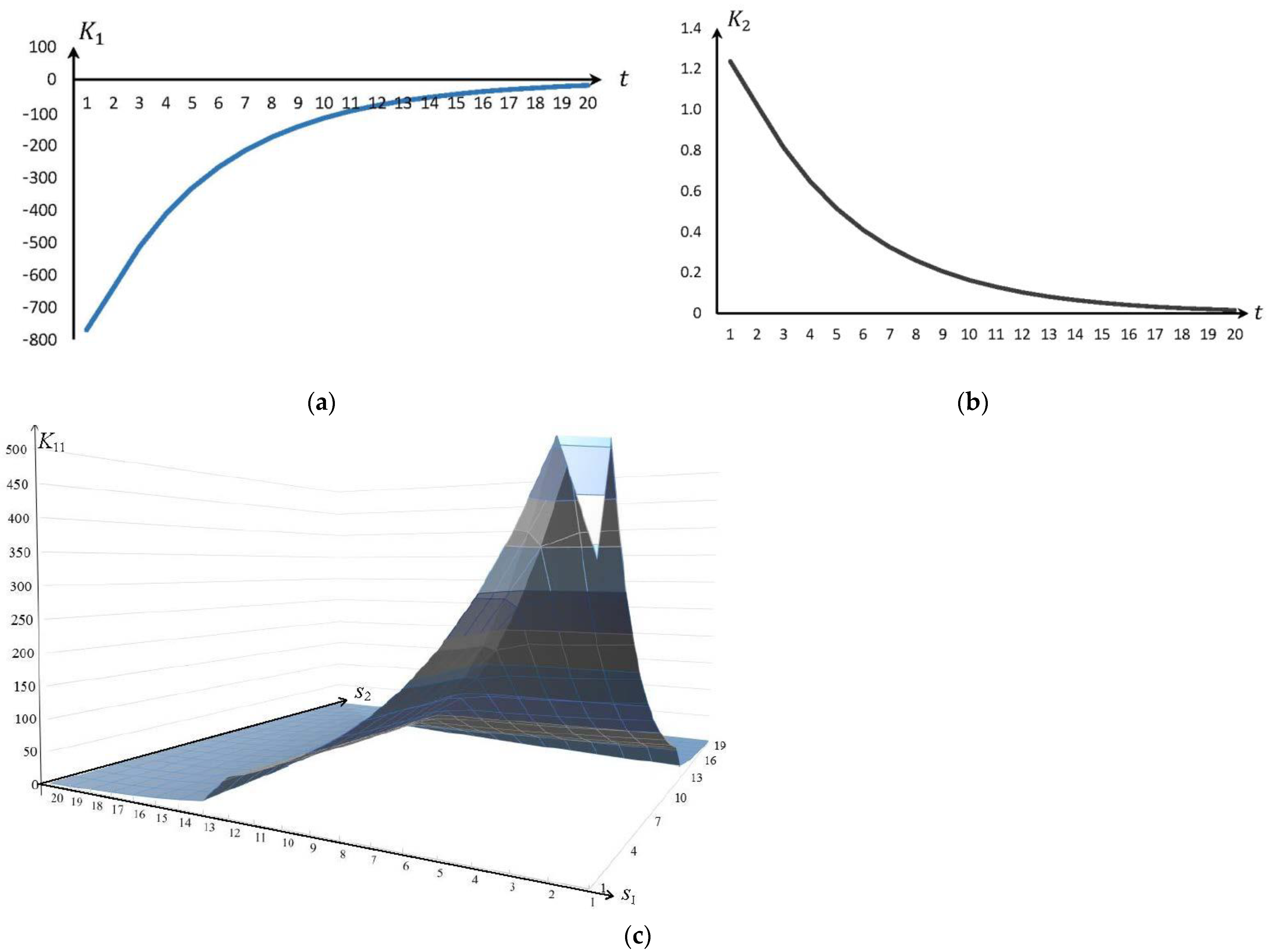
The identification of the mesh analogs of Volterra kernels tuned to test signals with amplitudes of 25% of the initial values of $D_0=0.16$ kg/s, $Q_0=100$ kW was carried out using the technique [42,44] for $T=40$ s, $h=1$ s. Figure 3 shows mesh analogs for $K_1$, $K_2$, $K_{11}$ characterizing the influence of $\Delta D(t)$ and $\Delta Q(t)$ on the change of $\Delta i(t)$. Kernels were identified on the discrete mesh with the step $h=1$ using responses $\Delta i(t)$ to test signals of the form Equation (5) with amplitudes equal to 25% of the initial values. For simplicity, $T=20$ s.

Additionally, when drafting the initial data for the identification of kernels, we take into account conditions of the form of Equations (8)–(11) following from the necessary and sufficient conditions for the solvability of the corresponding integral equations in the required functions’ classes. Note that in this case, we do not consider conditions ${\alpha }_{1,2}+{\alpha }_{2,2}=0$, ${\gamma }_{1,2}+{\gamma }_{2,2}=0$ from Equation (8), used to identify $K_{22}$ and $K_{122}$, respectively, as well as condition ${\stackrel{⌢}{\alpha }}_{1,2}+{\stackrel{⌢}{\alpha }}_{2,2}+{\stackrel{⌢}{\alpha }}_{3,2}=0$ from Equation (9), used to identify $K_{222}$. Let signals have the form:

$$x_1^{{\zeta }_1}(t)={\zeta }_{1}e(t), x_2^{{\zeta }_2}(t)={\zeta }_{2}e(t), t\in [0,T],$$

(15)

where ${\zeta }_1=25\%D_0=0.04$ kg/s, ${\zeta }_2=25\%Q_0=25$ kW, on which we will carry out the verification of mesh analogs of Equations (12) and (13). The responses of the constructed mesh analogs of the quadratic Equation (12) and cubic Equation (13) Volterra polynomials give a zero residual with the response of the simulation model Equation (3) to input signals of the form Equation (15).

An analysis of the computational experiment’s results showed that violation of the constraints of Equations (8)–(11) on the amplitudes used to identify Volterra kernels leads to the appearance of a nonzero error. In this case, various situations are possible. We will consider them in order of degradation in modeling accuracy.

Let equalities Equations (8)–(10) hold for a fixed value of $i=1$ (i.e., ${\alpha }_{1,1}+{\alpha }_{2,1}=0$, ${\stackrel{⌢}{\alpha }}_{1,1}+{\stackrel{⌢}{\alpha }}_{2,1}+{\stackrel{⌢}{\alpha }}_{3,1}=0$, ${\beta }_{k,1}^2={\alpha }_{k,1}^2$, ${\gamma }_{k,1}^2={\alpha }_{k,1}^2$). Violation of equality ${\beta }_{k,2}^2={\alpha }_{k,2}^2$ from Equation (11) does not influence the accuracy of the quadratic and cubic models for actions of the form Equation (15) (including arbitrary values of ${\zeta }_2$) due to the linearity of Equation (3) concerning $\Delta Q(t)$.

Now, let equalities of the form Equations (8)–(10) as well as Equation (11) for $i=2$ (i.e., ${\beta }_{k,2}^2={\alpha }_{k,2}^2$ and ${\gamma }_{k,2}^2={\alpha }_{k,2}^2$) hold, except for ${\beta }_{k,1}^2={\alpha }_{k,1}^2$ or ${\gamma }_{k,1}^2={\alpha }_{k,1}^2$. Then, on the signals in Equation (15), the residual between responses $y_2(t)$, $y_3(t)$ of integral models and $y_{et}(t)$ will be nonzero. Taking into account that the actions Equation (15) were used in identifying the Volterra kernels, a nonzero residual of modeling on the same signals means a defect in the identification of the integral models.

Table 1. Error values ${\epsilon }_1$ (%). Amplitudes ${\beta }_1$, ${\beta }_2$ were used to identify the nonsymmetric kernel, $K_{12}$.

	${\mathit{\beta }}_1$	0.0394	0.0396	0.0398	0.0400	0.0402	0.0404	0.0406
${\mathit{\beta }}_2$
24		15.929	10.487	5.013	0.000	6.034	11.605	17.209
25		14.896	9.798	4.667	0.000	5.687	10.911	16.166
26		13.942	9.161	4.348	0.000	5.367	10.270	15.204

gives the error values for signals Equation (15) in the case of violation of the equality in Equation (8). The calculations were carried out with double precision using a quadratic integral model, Equation (12). It can be seen from the table that the error ${\epsilon }_1$ decreases as ${\beta }_1$ approaches the required value of 0.04, while ${\epsilon }_1=0.000$% for ${\beta }_1=0.04$. This tendency is not obvious in the case of an arbitrary input signal.

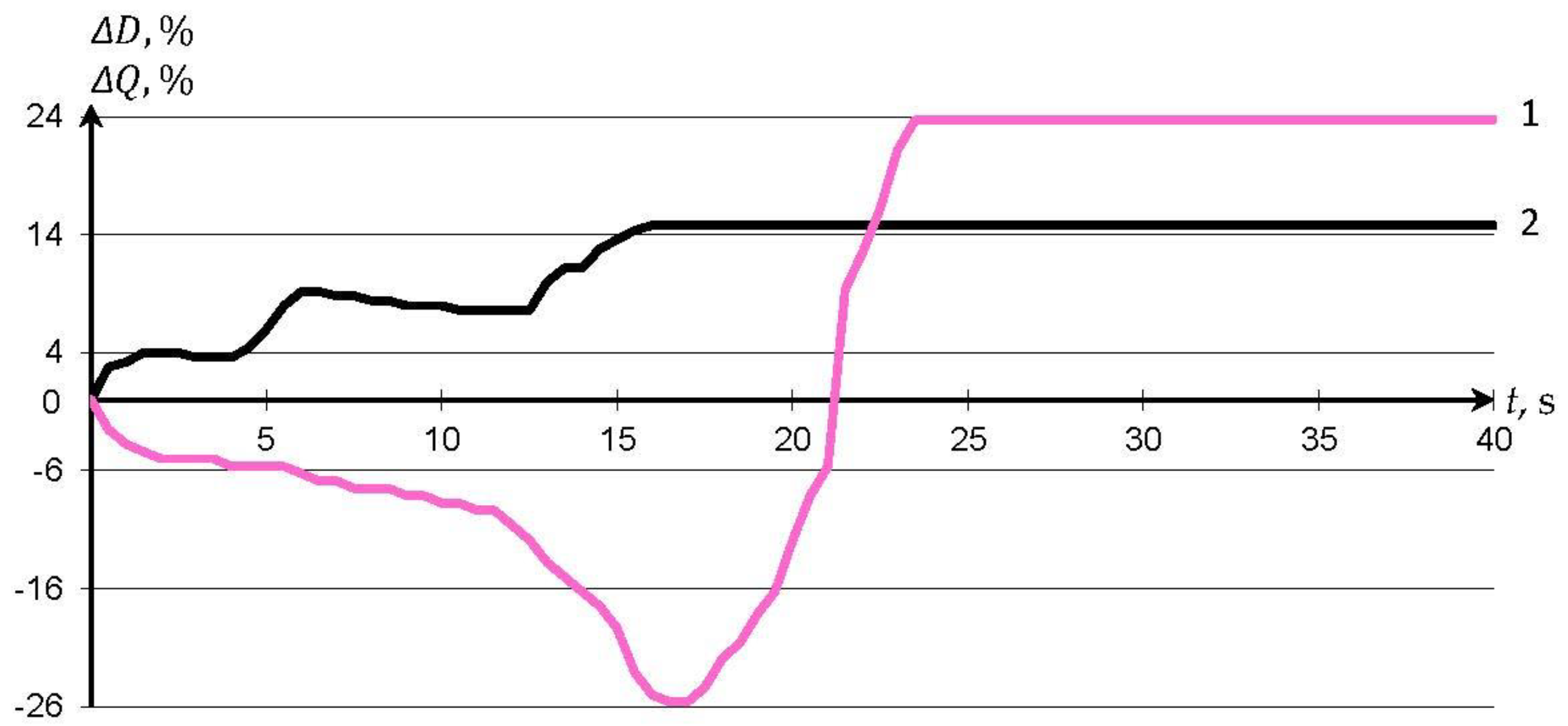
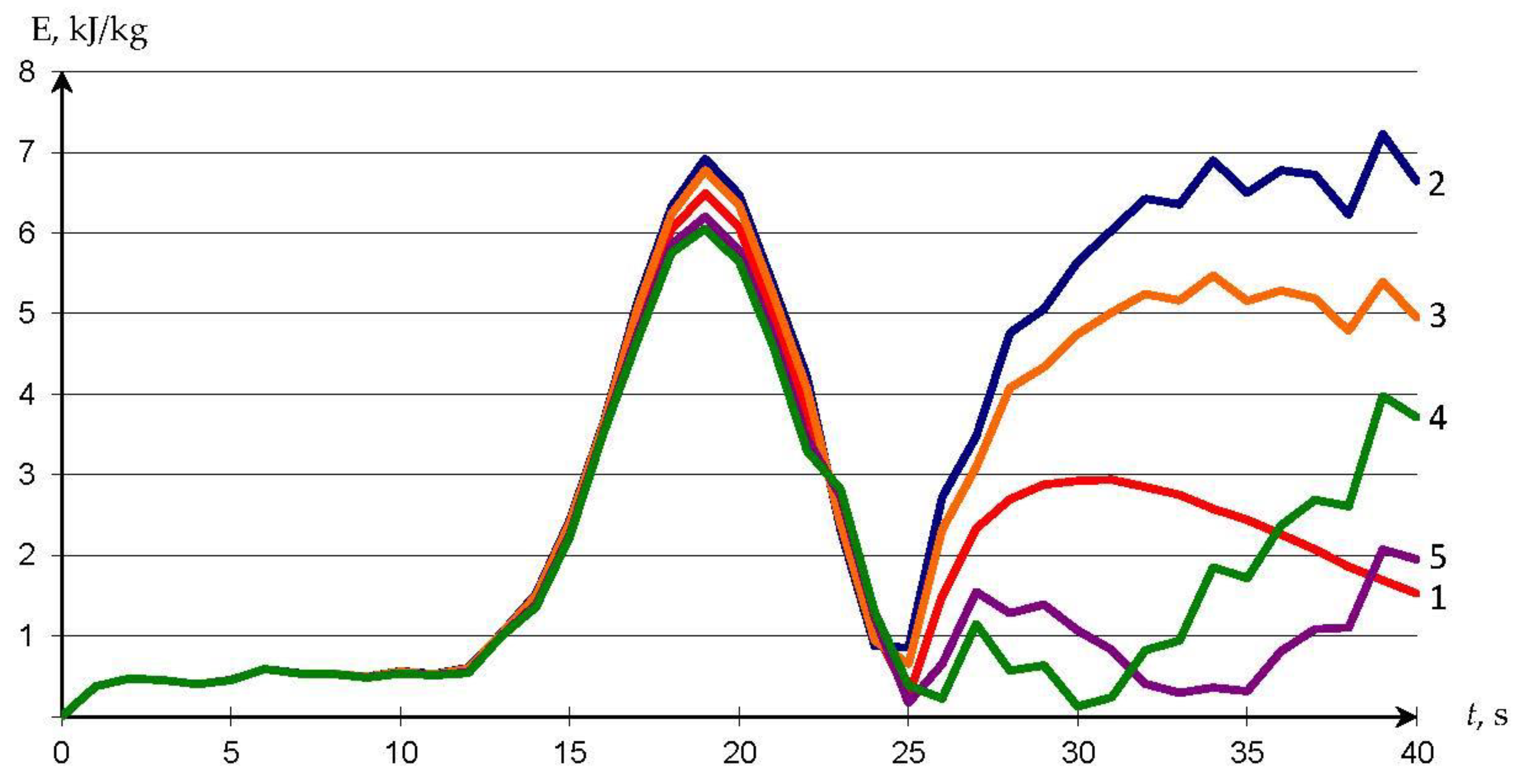
We illustrate this situation for the input actions shown in Figure 4, where line 1 corresponds to $\Delta D(t)$ and line 2 to $\Delta Q(t)$. Figure 5 shows graphics for residual $\mathrm{E}(t)=\left|y_2(t)-y_{et}(t)\right|$, $t\in [0,40]$, for fixed values ${\beta }_1$, ${\beta }_2$. Here, line 1 corresponds to the values of ${\beta }_1=25\%D_0=0.04$ kg/s and ${\beta }_2=25\%Q_0=25$ kW, so condition ${\beta }_{k,1}^2={\alpha }_{k,1}^2$ holds.

In this case, at $t_1=19$, the maximum error $\underset{t\in [0,T]}{\max }\mathrm{E}(t)=6.493$ is reached, which is 2.845% of $y_{et}(t_1)$. The rest of the graphs were obtained in violation of the limit on the value of ${\beta }_1$, where at ${\beta }_2=25$, number 2 marks the graph for ${\beta }_1=0.0385$, 3—for ${\beta }_1=0.039$, 4—for ${\beta }_1=0.041$, 5—for ${\beta }_1=0.0415$. In this case, $\underset{t\in [0,T]}{\max }\mathrm{E}(t)=7.226$ is reached at point $t_2=39$ (see Figure 5, graph 2), and is 16.741% of $y_{et}(t_2)$. Note that when $\Delta D(t)$ reaches a constant (see Figure 4, $t\ge 23$ s), then the nature of the change in errors (see Figure 5, graphs 2–5) of models, constructed with violation of the connectivity conditions for the test signals’ amplitudes, does not correspond to the dynamics of the residual (see Figure 5, graph 1) obtained when the required conditions are met. Note that the worst of the considered situations occurs when ${\alpha }_{1,1}+{\alpha }_{2,1}=r\ne 0$ from Equation (8) leads to a simultaneous violation of equalities (11). In particular, under the action of the form Equation (15), the error Equation (14) of the response of the cubic model is ${\epsilon }_2=3.943$%, even for $r={10}^{-5}$. Thus, the fulfilment of constraints Equations (8)–(11) on the test signals’ amplitudes used in the Volterra kernels’ identification significantly influences the simulation accuracy.

4. Volterra Polynomial Equations of the First Kind in the Problem of Identifying the Input Signals of a Dynamic System

Now we assume that the construction of an integral model in the Volterra polynomial form was completed. We consider the problem of identifying input signals $x(t)={(x_1(t),x_2(t),\dots ,x_p(t))}^T$, which is reduced to solving Volterra polynomial equations of the first kind for known Volterra kernels $K$ and response $y(t)={(y_1(t),y_2(t),\dots ,y_p(t))}^T$. This statement is associated with the problem of automatic regulation of technical objects [45], (p. 242). The theory of such equations has been studied relatively recently [46], while their unified terminology is still lacking in the scientific literature. In particular, these equations are called “multilinear Volterra equations” [46], “bilinear integral equations” [47,48], and “multiple integral equations” [49,50]. In what follows, we will call the equations under consideration “polynomial” [51], since the $N$th term of polynomial $P_N$ is an $N$-power integral operator [31].

The theory and numerical methods for solving the polynomial Equation (1) for $N=1$ and $N>1$ have significant differences. In a series of papers [42,46,47,51,52], the specificity of Equation (1) for $p=1$ is studied in detail, which for $N>1$, consists of the locality of the solution to the equation in $C_{[0,T]}$. Here, the locality is the smallness of the right endpoint of segment $[0,T]$. A method for obtaining estimates for solutions to some special nonlinear integral inequalities that for $N>1$ play for Equation (1) the same role as the Grönwall–Bellman inequality for a linear Volterra equation of the first kind was presented for the first time in [42]. Numerical methods for solving polynomial equations for $N=2$ based on cubature formulas for middle rectangles are constructed in [47]. Further research was aimed at developing the theory and numerical methods for solving systems of polynomial Equation (1) for $p=2$, $N=2,3$ based on the Newton-Kantorovich method [53,54,55], as well as the practical method of using the developed approaches as applied to Equation (3) in the problem of stabilizing the enthalpy $\Delta i(t)$ by the formation of the control input action $\Delta D(t)$ [42,44,56].

Additionally, consider the problem Equations (1) and (2) with an arbitrary finite value $p$ and $N=2$. In contrast to the results indicated in this section, we will assume that the input signals $x(t)={(x_1(t),x_2(t),\dots ,x_p(t))}^T$ are unknown and, as before, the output signals $y(t)={(y_1(t),y_2(t),\dots ,y_p(t))}^T$and the Volterra kernels $K$ are given. In this case, we have a system of integral equations of the first kind of the form

$$y(t)=V[Z]={\displaystyle \underset{0}{\overset{t}{\int }}K(t,s_1)x(s_1)d{s}_1+Z}[x],$$

(16)

where $K(t,s_1)$ is a $(p\times p)$-matrix, $x(t)$ and $y(t)$ are the unknown and given $p$-dimensional vector-functions, and the operator $Z[x]$ is defined by the rule

$$\begin{array}{c}Z[x]={\displaystyle \underset{0}{\overset{t}{\int }}{\displaystyle \underset{0}{\overset{t}{\int }}[}}{\displaystyle \sum _{j_1=1}^p{L}_{j_1}^1(t,s_1,s_2)x_1(s_1)x_{j_1}(s_2)+}{\displaystyle \sum _{j_2=1}^p{L}_{j_2}^2(t,s_1,s_2)x_2(s_1)x_{j_2}(s_2)+}\\ +{\displaystyle \sum _{j_3=3}^p{L}_{j_3}^3(t,s_1,s_2)x_3(s_1)x_{j_3}(s_2)}+\dots +{\displaystyle \sum _{j_{p-1}=p-1}^p{L}_{j_{p-1}}^{p-1}(t,s_1,s_2)x_p(s_1)x_{j_{p-1}}(s_2)}+\\ +L_{j_p}^p(t,s_1,s_2)x_p(s_1)x_{j_p}(s_2)]d{s}_{1}d{s}_2,\end{array}$$

(17)

where $j_m=\overline{1,m}$. In formula (17), $L_{j_m}^m(t,s_1,s_2)$ are $p$-dimensional vector-functions, that is, $L_{j_m}^m(t,s_1,s_2)={\left(Z_{j_{m}1}^m(t,s_1,s_2),Z_{j_{m}2}^m(t,s_1,s_2),\dots ,Z_{j_{m}p}^m(t,s_1,s_2)\right)}^T$ are smooth enough for further reasoning.

If:

$$\det K(t,t)\ne 0 \forall \hspace{0.17em}t\in [0,T],$$

(18)

in Equation (16), then the study of such systems for the existence of a unique solution in various classes of functions is carried out by analogy with Volterra integral equations of the first kind (see, for example, [57] and others). To do this, it is sufficient to differentiate the system Equation (16) with respect to $t$ and rewrite the obtained result in the form of a system of the second kind, and this is possible due to condition Equation (18).

If condition Equation (18) is not satisfied for the problem Equation (16), then the standard approaches do not give the desired result—a system of the second kind, since we have a system of integral equations with an identically degenerate matrix in front of the main part after differentiation. Such problems have the fundamental differences from systems of the type of Equation (16), with the condition in Equation (18). They inherit from the integral equation of the first kind with the condition ${K_{t^j}^{(j)}(t,s_1)|}_{s_1=t}\ne 0$, where $j$ is a non-negative integer, the instability to small perturbations $y(t)$ in the metric $C_{[0,T]}^j$ and the absence of a solution in the class of continuous functions under ${y^{(m)}(t)|}_{t=0}\ne 0$, $m=0,1,\dots ,j$.

We demonstrate the specifics and properties of Equation (16) with condition Equation (18) using the simplest examples, namely, systems Equation (16), for which the operator $Z[x]$ is identically zero. In this case, we have the system of Volterra integral equations of the first kind

$$y(t)={\displaystyle \underset{0}{\overset{t}{\int }}K(t,s)x(s)ds,\hspace{0.17em}\hspace{0.17em}\hspace{0.17em}0\le s\le t\le T},$$

(19)

where $K(t,s)$ is a $(p\times p)$-matrix, $y(t)$, $x(t)$ are the given and unknown $p$-dimensional vector-functions, and $\det K(t,t)\equiv 0$.

Example 1.

$${\displaystyle \underset{0}{\overset{t}{\int }}\left(\begin{array}{ccc}t-s& {\phi }_1(s)& 0\\ 0& t-s& {\phi }_2(s)\\ 0& 0& t-s\end{array}\right)\left(\begin{array}{c}{x}_1(s)\\ x_2(s)\\ x_3(s)\end{array}\right)ds=\left(\begin{array}{c}0\\ 0\\ y(t)\end{array}\right)},$$

(20)

where $y(t)$, ${\phi }_1(t)$ and ${\phi }_2(t)$ are the given functions that have the required smoothness. From the third equation in Equation (20), we have

$$x_3(t)=y^{″}(t).$$

(21)

Substituting this expression into the second equation in Equation (20), we obtain

$${\displaystyle \underset{0}{\overset{t}{\int }}(t-s)}{x}_2(s)ds=-{\displaystyle \underset{0}{\overset{t}{\int }}{\phi }_2(s)}{x}_3(s)ds$$

(22)

or, taking into account Equation (21) and differentiating twice Equation (22), we have

$$x_2(t)=-{\left({\phi }_2(t)y^{″}(t)\right)}^{\prime }.$$

(23)

By analogy, substituting Equation (23) into the first equation of system Equation (20), we have

$$x_1(t)={\left({\phi }_1(t){\left({\phi }_2(t)y^{″}(t)\right)}^{\prime }\right)}^{\prime }.$$

(24)

Thus, system Equation (20) has a unique solution, which is found by Formulas (21)–(24).

The rank of the matrix $K(t,t)$ can be variable, but this fact does not mean the presence of singular points.

Example 2. Consider the system

$${\displaystyle \underset{0}{\overset{t}{\int }}\left(\begin{array}{cc}1& a(t-s)\\ b(t-s)& c{(t-s)}^2\end{array}\right)\left(\begin{array}{c}{x}_1(s)\\ x_2(s)\end{array}\right)ds=\left(\begin{array}{c}0\\ 0\end{array}\right)\hspace{0.17em}},$$

where $a$, $b$, $c$ are scalar. This example has only the trivial solution, if $2c-ab\ne 0$. In the case of $2c-ab=0$ and $a\ne 0$, this example has the solution set of the form $x(t)={\left(v(t)-\frac{v^{\prime }(t)}{a}\right)}^T$, where $v(t)$ is a continuously differentiable function.

Another feature of systems, Equation (19), is the instability to small perturbations of the input data in an arbitrarily smooth metric.

Example 3. Consider a system

$${\displaystyle \underset{0}{\overset{t}{\int }}\left(\begin{array}{cc}t-s& 1\\ \epsilon (t-s)& t-s\end{array}\right)\left(\begin{array}{c}{x}_1(s)\\ x_2(s)\end{array}\right)ds=\left(\begin{array}{c}\epsilon t\\ 0\end{array}\right)\hspace{0.17em}},$$

(25)

where $\epsilon$ is a small scalar parameter. If $\epsilon =0$, the system Equation (25) has only the trivial solution. If $\epsilon \ne 0$, then, twice differentiating the second Equation in (25), we have

$$x_1(t)=-\frac{x_2(t)}{\epsilon }.$$

Differentiating the first equation in (25), we obtain:

$${\displaystyle \underset{0}{\overset{t}{\int }}{x}_1(s)ds}+x_2(t)=\epsilon ,$$

hence, $x_2(0)=\epsilon$ and $x_1(t)+{x^{\prime }}_2(t)=0$.

Given that $x_2(0)=\epsilon$ and $x_1(t)=-\frac{x_2(t)}{\epsilon }$, we have $x_2(t)=\epsilon \exp (t/\epsilon )$. For $\epsilon >0$, it follows that ${\Vert x_2(t)\Vert }_{C_{[0,T]}}\to \infty$, when $\epsilon \to 0$.

Here is another example that contains a singular point. The solution set passes through this point.

Example 4. Consider a problem

$${\displaystyle \underset{0}{\overset{t}{\int }}\left(\begin{array}{cc}s-2(t-s)& 1+t-2s\\ t-s& t-s\end{array}\right)\left(\begin{array}{c}{x}_1(s)\\ x_2(s)\end{array}\right)ds=\left(\begin{array}{c}0\\ 0\end{array}\right)\hspace{0.17em}}.$$

(26)

Differentiating the second equation in (26) twice with respect to $t$, we obtain $x_1(t)+x_2(t)=0$, or

$$x_1(t)=-x_2(t).$$

(27)

Substituting this expression into the first equation in (26), we have the integral equation with respect to $x_1(t)$

$${\displaystyle \underset{0}{\overset{t}{\int }}(-1+5s-3t)x_1(s)ds=0}.$$

Differentiating this equation, we obtain

$$(2t-1)x_1(t)-3{\displaystyle \underset{0}{\overset{t}{\int }}{x}_1(s)ds=0}.$$

(28)

When $T>\frac{1}{2}$, Equation (28) is the Volterra integral equation of the third kind. The solution set of the form

$$x_1(t)=C\sqrt{2t-1},\hspace{0.17em}\hspace{0.17em}\hspace{0.17em}\hspace{0.17em}\hspace{0.17em}t\ge \frac{1}{2},$$

passes through the point $t=\frac{1}{2}$, where $C$ is an arbitrary constant.

Thus, taking into account Equation (27), when $T>\frac{1}{2}$, the solution to problem Equation (26) is

$$x_1(t)=\{\begin{array}{cc}0,\hfill & t\in [0,\raisebox{1ex}{$1$}\!\left/ \!\raisebox{-1ex}{$2$}\right.],\hfill \\ C\sqrt{2t-1},& t\in [\raisebox{1ex}{$1$}\!\left/ \!\raisebox{-1ex}{$2$}\right.,T],\hfill \end{array}\hspace{0.17em}\hspace{0.17em}\hspace{0.17em}{x}_2(t)=\{\begin{array}{cc}0,& t\in [0,\raisebox{1ex}{$1$}\!\left/ \!\raisebox{-1ex}{$2$}\right.],\hfill \\ -C\sqrt{2t-1},& t\in [\raisebox{1ex}{$1$}\!\left/ \!\raisebox{-1ex}{$2$}\right.,T].\hfill \end{array}$$

These examples show the fundamental difference between the systems of Equation (19) with the condition $\det K(t,t)\ne 0$ $\forall t\in [0,T]$ from the problems with the condition $\det K(t,t)\equiv 0$.

We give sufficient conditions for the existence of the continuously differentiable solution of the system in Equation (16) with the condition in Equation (18).

Statement 1. 

Suppose that the following conditions hold for problem Equation (16):

(1)

The elements of$y(t)$,$K(t,s_1)$ $L_{j_m}^m(t,s_1,s_2)$(see Equation (17)) are twice continuously differentiable functions with respect to the set of arguments,

(2)

$y(0)=0$,

(3)

$rank\hspace{0.17em}K(0,0)=rank\{K(0,0)|y^{\prime }(t){|}_{t=0}\}$,

(4)

$rank\hspace{0.17em}K(t,t)=r=\mathrm{const}$ $\forall t\in [0,T]$,

(5)

$\det \left(\lambda K(t,t)+{{K^{\prime }}_t(t,s)|}_{s=t}\right)=a_0(t){\lambda }^r+a_1(t){\lambda }^{r-1}+\dots +a_r(t)$,

where$\lambda$are scalar,$a_0(t)$,$a_1(t)$, …,$a_r(t)$are functions, and$a_0(t)\ne 0$ $\forall t\in [0,T]$.

Then the original problem has a unique continuous solution.

Proof of Statement 1 

The proof of this fact is based on the results of the articles [58,59].

Let us comment on the conditions of Statement 1. The first condition is the standard condition for the smoothness of the input data, since, in the proof, we need to differentiate Equation (16) twice and then compose a linear combination. The second and third ones are the conditions for the correct assignment of the initial data $y(0)$. These conditions follow directly from the Rouche–Capelli theorem, that is, substituting into Equation (16) $t=0$, we obtain SLAE $y(0)=0$ (the second condition). Differentiating the original problem and substituting $t=0$, we have SLAE:

$$K(0,0)x(0)={y^{\prime }(t)|}_{t=0}.$$

Finally, conditions (4) and (5) guarantee the absence of singular points through which several solutions can pass, or in which the solution is discontinuous. □

To illustrate the fourth condition, it is sufficient to consider the integral Equation (19), where $K(t,s)$ and $y(t)$ are functions, and $K(t_j,t_j)=0$, $t_j\in [0,T]$. In this case, after differentiation, we have the integral equation of the third kind,

$$y^{\prime }(t)=K(t,t)x(t)+{\displaystyle \underset{0}{\overset{t}{\int }}{K^{\prime }}_t(t,s)x(s)ds},0\le s\le t\le T.$$

(29)

Assuming in (29) $K(t,s)=at+bs$, where $a$ and $b$ are scalar, it is possible to choose such values of $a$ and $b$, that this equation have either a discontinuous solution or non-unique solution. In this case, the fourth condition of Statement 1 is violated.

Let us verify in Equation (26) the conditions (4) and (5). The fourth condition:

$$rank\hspace{0.17em}K(t,t)=rank\left(\begin{array}{cc}t& 1-t\\ 0& 0\end{array}\right)=1=\mathrm{const}$$

holds. The fifth condition is:

$$\begin{array}{l}\det \left(\lambda K(t,t)+{{K^{\prime }}_t(t,s)|}_{s=t}\right)\hspace{0.17em}=\det \left[\left(\begin{array}{cc}\lambda t& \lambda \left(1-t\right)\\ 0& 0\end{array}\right)+\left(\begin{array}{cc}-2& 1\\ 1& 1\end{array}\right)\right]=\\ =\det \left(\begin{array}{cc}\lambda t-2& \lambda \left(1-t\right)+1\\ 1& 1\end{array}\right)=(2t-1)\lambda -3.\end{array}$$

Here, $a_0(t)=2t-1$. This function vanishes when $t_1=\frac{1}{2}$, that is, when $t=t_1$, the fifth condition is violated, and the solution set of this example passes through this point.

A more general case of Equation (29) is

$$\phi (t)=A(t)x(t)+{\displaystyle \underset{0}{\overset{t}{\int }}K(t,s)x(s)ds},$$

(30)

where $A(t)$, $K(t,s)$ are the given $(p\times p)$-matrices, $\phi (t)$ and $x(t)$ are the given and unknown$p$-dimensional vector functions. It is assumed that

$$\det A(t)\equiv 0.$$

(31)

Equation (30) with condition (31) has been the focus of attention of specialists relatively recently, since the late 1980s to the early 1990s. The first article on this topic was published in 1987 [60]. Since then, no more than 50 papers have been published on the qualitative theory and numerical solution of systems (30) with condition (31). Such systems were called the “integral analogs of singular systems of ordinary differential equations” in [60], “integral equations of the fourth kind” in [61] and [62], and “singular systems of integral equations” in [63]. Now, these systems are referred to as “integral-algebraic equations” (IAEs) [64]. The problems of constructing numerical methods for solving IAEs are noted in articles [65,66,67] and monographs [68,69]. A fairly complete bibliography is presented in [70,71].

5. Conclusions

When solving inverse problems in power engineering, nonclassical integral equations of the Volterra type arise. At the present time, the theoretical apparatus for studying such equations is not complete and requires further development. This paper presents mathematical tools for solving problems, associated with the application of the Volterra integro-power series. The effectiveness of using the previously obtained theoretical results is illustrated by the practical example in modeling the nonlinear dynamics of an element of a heat exchange unit.

The classes of nonlinear systems of integral equations of the first kind were identified that have a unique sufficiently smooth solution (under the certain conditions for the vector function $y(t)$ and the input data). The sufficient conditions are formulated in terms of matrix pencils. The presented new theoretical results are due to the problems arising in the study of heat power engineering objects, and also have independent significance.

In the future, it is planned to construct and justify numerical methods for solving such systems. These algorithms are supposed to be based on the extrapolation formulas [67], which have performed well when solving IAEs Equation (30), on the special quadrature formula of the midpoint type [58,59], and on the collocation-variational approach that was proposed for the numerical solution to differential-algebraic equations [72,73,74,75].

References

- Merenkov, A.P.; Rudenko, Y.N. Methods for Investigation and Management of Energy Systems; Nauka: Novosibirsk, Russia, 1987. [Google Scholar]
- Zhou, H.; Chen, C.; Lai, J.; Lu, X.; Deng, Q.; Gao, X.; Lei, Z. Affine nonlinear control for an ultra-supercritical coal fired once-through boiler-turbine unit. Energy 2018, 153, 638–649. [Google Scholar] [CrossRef]
- Shen, C.; Zhao, Y.; Li, Y. Design of Boiler Steam Temperature Control System. Therm. Sci. Eng. 2018, 1. [Google Scholar] [CrossRef]
- Shnayder, D.A.; Kazarinov, L. Energy efficient predictive control of complex manufacturing processes. Upr. Bol’shimi Sist. 2011, 32, 221–240. [Google Scholar]
- Zhang, X.; Ye, Y.; Wang, H.; An, X. A new method for boiler combustion calculation. Earth Environ. Sci. 2018, 199, 154–157. [Google Scholar] [CrossRef]
- Sit, M.L.; Patsiuk, V.I.; Juravliov, A.A.; Burciu, V.I.; Timchenko, D.V. Control of Heat Exchanger with Variable Heat Transfer Surface Area. Probl. Energ. Reg. 2019, 1, 90–101. [Google Scholar]
- Filimonova, A.A.; Barbasova, T.; Shnayder, D.; Basalaev, A. Heat Supply Modes Optimization Based on Macromodeling Technology. Energy Procedia 2017, 111, 710–719. [Google Scholar] [CrossRef]
- Juravliov, A.A.; Shit, M.L.; Poponova, O.B.; Shit, B.M. Design of the control law of the steam drum boiler level taking into consideration energy economy. Probl. Energ. Reg. 2005, 1, 43–52. [Google Scholar]
- Kurbatsky, V.; Tomin, N. Forecasting prices in the liberalized electricity market using the hybrid models. In Proceedings of the 2010 IEEE International Energy Conference, Manama, Bahrain, 18–22 December 2010; pp. 363–368. [Google Scholar] [CrossRef]
- Hernandez, L.; Baladrón, C.; Aguiar, J.M.; Carro, B.; Sanchez-Esguevillas, A.J.; Lloret, J. Short-Term Load Forecasting for Microgrids Based on Artificial Neural Networks. Energies 2013, 6, 1385–1408. [Google Scholar] [CrossRef] [Green Version]
- Alam, M.M.; Ahmed, M.F.; Jang, Y.M.; Islam, M.R. Automatic Control Approach of Reactive Power Compensation of Smart Grid. In Proceedings of the 2020 International Conference on Artificial Intelligence in Information and Communication (ICAIIC), Fukuoka, Japan, 19–21 February 2020; pp. 716–719. [Google Scholar] [CrossRef]
- Vilchis-Rodriguez, D.; Levi, V.; Gupta, R.; Barnes, M. Feasibility Analysis of the Probabilistic Modelling of LCC Based HVDC Equipment Ageing Using Public Data. In Proceedings of the 10th International Conference PEMD 2020, Nottingham, UK, 1–3 December 2020. [Google Scholar]
- Osak, A.B.; Panasetsky, D.A.; Buzina, E.Y. Analysis of the emergency control and relay protection structures approached from the point of view of EPS reliability and survivability by taking into account cybersecurity threats. E3S Web Conf. 2019, 139, 01029. [Google Scholar] [CrossRef]
- Shokouhandeh, H.; Ghaharpour, M.R.; Lamouki, H.G.; Pashakolaei, Y.R.; Rahmani, F.; Imani, M.H. Optimal Estimation of Capacity and Location of Wind, Solar and Fuel Cell Sources in Distribution Systems Considering Load Changes by Lightning Search Algorithm. In Proceedings of the XIV 2020 IEEE Texas Power and Energy Conference (TPEC), College Station, TX, USA, 6–7 February 2020. [Google Scholar]
- Khamisov, O.O.; Chernova, T.S.; Bialek, J.W.; Low, S.H. Corrective Control: Stability Analysis of Unified Controller Combining Frequency Control and Congestion Management. 2018. Available online: https://arxiv.org/abs/1806.10303 (accessed on 29 June 2021).
- Ayalew, F.; Hussen, S.; Pasam, G.K. Optimization Techniques in Power System: Review. Int. J. Eng. Appl. Sci. Tech. 2018, 3, 8–16. [Google Scholar]
- Zadeh, L.A. Fuzzy Sets. In Fuzzy Sets; Defense Technical Information Center: Fort Belvoir, VA, USA, 1964; Volume 3, pp. 338–353. [Google Scholar]
- Haykin, S. Neural Networks and Learning Machines; Pearson Prentice Hall: Hoboken, NJ, USA, 1999. [Google Scholar]
- Volterra, V. A Theory of Functionals and of Integral and Integro-Differential Equations; Dover Publications: New York, NY, USA, 1959; ISBN 0486442845. [Google Scholar]
- Cheng, C.M.; Peng, Z.K.; Zhang, W.M.; Meng, G. Volterra-series-based nonlinear system modeling and its engineering applications: A state-of-the-art review. Mech. Syst. Signal Process. 2017, 87, 364–430. [Google Scholar] [CrossRef]
- Stegmayer, G.; Pirola, M.; Orengo, G.; Chiotti, O. Towards a Volterra Series Representation from a Neural Network Model. WSEAS Trans. Syst. 2004, 3, 432–437. [Google Scholar]
- Licheng, J.; Fang, L.; Qin, X. Volterra Feedforward Neural Networks: Theory and Algorithms. J. Syst. Eng. Electr. 1996, 7, 1–12. [Google Scholar]
- Ghanem, S.; Roheda, S.; Krim, H. Latent Code-Based Fusion: A Volterra Neural Network Approach. 2021. Available online: https://arxiv.org/pdf/2104.04829.pdf (accessed on 29 June 2021).
- Apartsyn, A.S.; Tairov, E.A.; Solodusha, S.V.; Khudyakov, D.V. Application of the Volterra integro-power series to modelling the heat-exchange dynamics. Proc. RAS Energy 1994, 3, 28–42. [Google Scholar]
- Shcherbinin, M.S. Optimization of Consumption of Power Resources of Turbo Compressor M-1 Ep-300 Using Programming and Computing Suite. Sci. Tech. Bull. OJSC NK Rosneft 2010, 3, 36–39. [Google Scholar]
- Suslov, K.V.; Gerasimov, D.O.; Solodusha, S.V. Smart Grid: Algorithms for Control of Active- Adaptive Network Components. In Proceedings of the 2015 IEEE Eindhoven PowerTech, Eindhoven, The Netherlands, 29 June–2 July 2015. [Google Scholar] [CrossRef]
- Fomin, О.; Marsi, M.; Pavlenko, V. Intelligent technology of nonlinear dynamics diagnostics using Volterra kernels moments. Int. J. Math. Models Methods Appl. Sci. 2016, 10, 158–165. [Google Scholar]
- Medvedew, A.; Fomin, O.; Pavlenko, V.; Speranskyy, V. Diagnostic features space construction using Volterra kernels wavelet transforms. In Proceedings of the 2017 9th IEEE International Conference on Intelligent Data Acquisition and Advanced Computing Systems: Technology and Applications (IDAACS), Bucharest, Romania, 21–23 September 2017; pp. 1077–1081. [Google Scholar] [CrossRef]
- Medina-Ramos, C.; Betetta-Gomez, J.; Carbonel-Olazabal, D.; Pilco-Barrenechea, M. System identification and MPC based on the Volterra-Laguerre model for improvement of the laminator systems performance. In Proceedings of the 2013 IEEE International Symposium Sensorless Control for Electrical Drives and Predictive Control of Electrical Drives and Power Electronics (SLED/PRECEDE), Munich, Germany, 17–19 October 2013. [Google Scholar] [CrossRef]
- Solodovnikov, V.V. Automatic Control Theory; Mashinostroenie: Moscow, Russia, 1969; Book 3, Part I. [Google Scholar]
- Boyd, S.; Chua, L.O.; Desoer, C.A. Analytical Foundations of Volterra Series. IMA J. Math. Control Inf. 1984, 1, 243–282. [Google Scholar] [CrossRef]
- Glushkov, V.M.; Ivanov, V.V.; Yanenko, V.M. Modeling of Developing Systems; Nauka: Moscow, Russia, 1983. [Google Scholar]
- Tairov, E.A. Nonlinear modeling of the dynamics of heat transfer in a channel with single phase coolant. Proc. RAS Power Eng. Transp. 1989, 1, 150–156. [Google Scholar]
- Magid, S.I.; Gerzhoi, I.P.; Rubashkin, A.S.; Krasheninnikov, V.V.; Vinogradova, T.A. Mathematical model of transient processes of a once-through boiler for a simulator for an operator of a 250 MW cogeneration power unit. Therm. Eng. 1985, 5, 34–38. [Google Scholar]
- Tairov, E.A.; Levin, A.A.; Zapov, V.V. Development of methods to simulate the dynamics of heat power engineering plants. Bull. ISTU 2011, 3, 117–123. [Google Scholar]
- Solodusha, S.V. Quadratic and cubic Volterra polynomials: Identification and application. Vestn. SPb Univ. Appl. Math. Comput. Sci. Control. Process. 2018, 14, 131–144. [Google Scholar] [CrossRef]
- Fedorova, A.N.; Fomin, A.A.; Pavlenko, V.D. The method of constructing multidimensional Volterra model of the oculo-motor apparatus. Electr. Comput. Syst. 2015, 19, 296–301. [Google Scholar] [CrossRef]
- Apartsyn, A.S. Nonclassical Volterra Equations of the First Kind in Integral Models of Dynamical Systems: Theory, Numerical Methods, Applications. Ph.D. Thesis, Irkutsk State University, Irkutsk, Russia, 23 June 2000. [Google Scholar]
- Apartsyn, A.S.; Solodusha, S.V. Test signal amplitude optimization for identification of the Volterra kernels. Autom. Remote Control 2004, 65, 464–471. [Google Scholar] [CrossRef]
- Apartsyn, A.S. Mathematical modelling of the dynamic systems and objects with the help of the Volterra integral series. In Proceedings of the EPRI-SEI Joint Seminar of Methods for Solving the Problems on Energy Power Systems Development and Control, Beijing, China, 21–26 September 1991; pp. 117–132. [Google Scholar]
- Solodusha, S.V.; Suslov, K.V.; Gerasimov, D.O. A New Algorithm for Construction of Quadratic Volterra Model for a Non-Stationary Dynamic System. IFAC Pap. OnLine 2015, 48, 982–987. [Google Scholar] [CrossRef]
- Apartsyn, A.S.; Solodusha, S.V.; Spiryaev, V.A. Modeling of Nonlinear Dynamic Systems with Volterra Polynomials: Elements of Theory and Applications. Int. J. Energy Optim. Eng. 2013, 2, 16–43. [Google Scholar] [CrossRef]
- Solodusha, S.V. Amplitudes of Test Signals for Identification of Volterra Kernels. In Proceedings of the 2018 International Conference on Industrial Engineering, Applications and Manufacturing (ICIEAM), Moscow, Russia, 15–18 May 2018; pp. 1–6. [Google Scholar] [CrossRef]
- Solodusha, S.V. Applications of nonlinear Volterra equations of the first kind to the control problem for heat exchange dynamics. Autom. Remote Control 2011, 72, 1264–1270. [Google Scholar] [CrossRef]
- Solodovnikov, V.V. Automatic Control Theory; Mashinostroenie: Moscow, Russia, 1969; Book 3, Part II. [Google Scholar]
- Apartsyn, A.S. Multilinear Volterra equations of the first kind. Autom. Remote Control 2004, 65, 263–269. [Google Scholar] [CrossRef]
- Apartsyn, A.S. On the convergence of numerical methods for solving a Volterra bilinear equations of the first kind. Comput. Math. Math. Phys. 2007, 47, 1323–1331. [Google Scholar] [CrossRef]
- Burt, P.M.S.; de Morais Goulart, J.H. Efficient Computation of Bilinear Approximations and Volterra Models of Nonlinear Systems. IEEE T Signal Process. 2018, 66, 804–816. [Google Scholar] [CrossRef] [Green Version]
- Belbas, S.A.; Bulka, Y. Numerical solution of multiple nonlinear Volterra integral equations. Appl. Math. Comput. 2011, 217, 4791–4804. [Google Scholar] [CrossRef] [Green Version]
- Belbas, S.A. Optimal control of second-order integral equations. arXiv 2019, arXiv:1904.06561. [Google Scholar]
- Apartsyn, A.S. Multilinear Volterra equations of the first kind and some problems of control. Autom. Remote Control 2008, 69, 545–558. [Google Scholar] [CrossRef]
- Apartsyn, A.S. Studying the polynomial Volterra equation of the first kind for solution stability. Autom. Remote Control 2011, 72, 1229–1236. [Google Scholar] [CrossRef]
- Solodusha, S.V. A class of systems of bilinear integral Volterra equations of the first kind of the second order. Autom. Remote Control 2009, 70, 663–671. [Google Scholar] [CrossRef]
- Solodusha, S.V. To the numerical solution of one class of systems of the Volterra polynomial equations of the first kind. Num. Anal. Appl. 2018, 11, 89–97. [Google Scholar] [CrossRef]
- Solodusha, S.V. Identification of input signals in integral models of one class of nonlinear dynamic systems. Bull. Irkutsk State Univ. Ser. Math. 2019, 30, 73–82. [Google Scholar] [CrossRef]
- Solodusha, S.V. Modeling heat exchangers by quadratic Volterra polynomials. Autom. Remote Control 2014, 75, 87–94. [Google Scholar] [CrossRef]
- Krasnov, M.L. The Integral Equations; Nauka: Moscow, Russia, 1975. [Google Scholar]
- Bulatov, M.V. Numerical solution of systems of integral equations of the first kind. Comput. Technol. 2001, 6, 3–8. [Google Scholar]
- Bulatov, M.V. Numerical solution of a system of Volterra equations of the first kind. Comput. Math. Math. Phys. 1998, 38, 585–589. [Google Scholar]
- Chistyakov, V.F. On singular systems of ordinary differential equations and their integral analogs. In The Lyapunov Function Method and Applications; Nauka: Novosibirsk, Russia, 1987; pp. 231–239. [Google Scholar]
- Bulatov, M.V.; Chistyakov, V.F. The Properties of Differential-Algebraic Systems and Their Integral Analogs; Memorial University of Newfoundland: St. John’s, NL, Canada, 1997; p. 35, preprint. [Google Scholar]
- Bulatov, M.V. On Nonlinear Systems of Integral Equations of the Fourth Kind. In Proceedings of the 11th Baikal International School-Seminar on Optimization Methods and Their Applications, Irkutsk, Russia, 5–12 July 1998; Volume 4, pp. 68–71. [Google Scholar]
- Brunner, H.; Bulatov, M. On Singular Systems of Integral Equations with Weakly Singular Kernels. In Proceedings of the 11th Baikal International School-Seminar on Optimization Methods and Their Applications, Irkutsk, Russia, 5–12 July 1998; Volume 4, pp. 64–68. [Google Scholar]
- Gear, C.W. Differential-Algebraic Equations, Indices, and Integral Algebraic Equations. SIAM J. Numer. Anal. 1990, 27, 1527–1534. [Google Scholar] [CrossRef]
- Hadizadeh, M.; Farahani, M.S. Direct Regularization for System of Integral-Algebraic Equations of index-1. Inverse Probl. Sci. Eng. 2018, 5, 728–743. [Google Scholar] [CrossRef]
- Pishbin, S. Error analysis of the ultraspherical spectral-collocation method for high-index IAEs. Int. J. Comp. Math. 2017, 94, 650–662. [Google Scholar] [CrossRef]
- Budnikova, O.S.; Bulatov, M.V. Numerical solution of integral-algebraic equations for multistep methods. Comput. Math. Math. Phys. 2012, 52, 691–701. [Google Scholar] [CrossRef]
- Brunner, H.; van der Houwen, P. The Numerical Solution of Volterra Equations; Elsevier Science Pub. Co.: Amsterdam, The Netherlands, 1986. [Google Scholar]
- Brunner, H. Collocation Methods for Volterra Integral and Related Functional Equations; Cambridge University Press: New York, NY, USA, 2004. [Google Scholar]
- Budnikova, O.S. Numerical Solution of Integral-Algebraic Equations for Multistep Methods; Moscow State University: Moscow, Russia, 2015. [Google Scholar]
- Botoroeva, M.N. Modeling Developing Systems Based on Volterra Integral Equations; Buryat State University: Buryatia, Russia, 2019. [Google Scholar]
- Bulatov, M.; Gorbunov, V.; Martynenko, Y.; Cong, N.D. Variational approaches to numerical solution of differential algebraic equations. Comput. Technol. 2010, 15, 3–13. [Google Scholar]
- Bulatov, M.V.; Rakhvalov, N.P.; Solovarova, L.S. Numerical solution of differential-algebraic equations using the spline collocation-variation method. Comput. Math. Math. Phys. 2013, 53, 284–295. [Google Scholar] [CrossRef]
- Bulatov, M.V.; Solovarova, L.S. Collocation-variation difference schemes for differential-algebraic equations. Math. Methods Appl. Sci. 2018, 41, 9048–9056. [Google Scholar] [CrossRef]
- Bulatov, M.; Solovarova, L. Collocation-variation difference schemes with several collocation points for differential-algebraic equations. Appl. Numer. Math. 2020, 149, 153–163. [Google Scholar] [CrossRef]
Figure 1.
Change in enthalpy under disturbance of water flow rate: (a) for a once-through boiler; (b) for the boiler unit economizer.
Figure 2.
Comparison of enthalpy graphs at dimensionless time (blue line is graph 1, green line is graph 2, black line is graph 3).
Figure 3.
Mesh analogs for the kernels: (a) ; (b) ; (c) .
Figure 4.
Input actions (line 1) and (line 2), %.
Figure 5.
Response error of quadratic integral models.