Analysis of Elastic–Plastic Problems Using the Improved Interpolating Complex Variable Element Free Galerkin Method

Abstract

A numerical model for the two-dimensional nonlinear elastic–plastic problem is proposed based on the improved interpolating complex variable element free Galerkin (IICVEFG) method and the incremental tangent stiffness matrix method. The viability of the proposed model is verified through three elastic–plastic examples. The numerical analyses show that the IICVEFG method has good convergence. The solutions using the IICVEFG method are consistent with the solutions obtained from the finite element method using the ABAQUS program. Moreover, the IICVEFG method shows greater computing precision and efficiency than the non-interpolating meshless methods.

1. Introduction

In the science and engineering fields, nonlinear elastic–plastic problems are very common, and are complicated due to the nonlinearity of the plastic state. In addition, the corresponding analytical solutions are difficult to be obtain [1,2,3]. Thus, it is important to study efficient and accurate computational models for solving nonlinear elastic–plastic problems, particularly those problems characterised by geometric [4,5,6] and material nonlinearities [7,8,9]. In recent years, the meshless method has played a great role in numerical simulation. Unlike conventional mesh-based numerical methods [10,11], the meshless method is built on discrete nodes, which does not cause mesh distortion. Therefore, the meshless method is more suitable for nonlinear large deformation and fracture problems, as well as complicated porous structures [12,13,14,15,16,17].

As a popular numerical computing method, the meshless method has developed various branches, such as the smoothed particle hydrodynamics method [18], the famous moving least squares (MLS) approximation [11], the reproducing kernel particle method [19], and so on. In this paper, we mainly study methods that improve upon the original MLS approximation in order to overcome shortcomings which lead to low efficiency and low accuracy [20,21,22]. The shortcomings include relying on numerous nodes, possessing a non-interpolating shape function, and possibly producing an ill-conditioned final discrete system.

To overcome inefficiency, complex variables were introduced into the MLS approximation, and the complex variable moving least squares (CVMLS) approximation was proposed [20]. Since the CVMLS approximation can use a complex variable to express the two directional variables, the CVMLS approximation has a higher computing efficiency [21,22]. However, this approximation lacks specific mathematical implications. Thus, the improved complex variable moving least squares (ICVMLS) approximation was proposed, which brings in a conjugated basis function and a new functional [23,24,25].

Identically to the MLS approximation, there are no interpolating features for the shape functions in the CVMLS and ICVMLS approximations [26,27,28,29]. Thus, on the foundation of the ICVMLS approximation, the interpolating property of the shape function was improved according to the following steps. First, to guarantee computing accuracy, a complete basis function is applied [30]. Second, the basis function is orthogonalized to obtain a set of new basis functions with a singular weight function [31]. Finally, based on these novel basis functions, a new interpolating shape function and interpolating trial function are derived. This new method was named the improved interpolating complex variable moving least squares (IICVMLS) method [30].

Combining the IICVMLS method with the integral weak forms of diverse problems, the corresponding improved interpolating complex variable element free Galerkin (IICVEFG) methods were presented. By virtue of the interpolating shape function in the IICVMLS method, the above meshless method is able to directly exert the essential boundary conditions, similarly to the finite element method. Thus, the derived final discrete system is more concise, which leads to greater computing efficiency and accuracy, in contrast to other non-interpolating complex variable meshless methods. Because of the above merits, the IICVEFG method has been widely applied to many potential problems, including the bending problems of Kirchhoff plates and even the pattern transformation of hydrogels, in which has displayed great computational advantages [30,32,33].

The intention of this paper is to build a more efficient and accurate numerical model for the two-dimensional nonlinear elastic–plastic problem based on the IICVEFG method, and to verify the viability of the proposed model. The detailed modelling process of the IICVEFG method is described, and the implementation process for solving the final discrete system is also presented. Through three numerical examples, the computational advantages of the IICVEFG method are demonstrated, in comparison with the ABAQUS program and other non-interpolating meshless methods.

2. Implementation of the Elastic–Plastic Problem Based on the IICVEFG Method

2.1. Brief Descriptions of the Two-Dimensional Elastic–Plastic Problem

Within the problem domain $\Omega$, the classic equilibrium equation of a two-dimensional elastic–plastic problem is [34]

$${\mathit{L}}^{\mathrm{T}}\dot{\mathit{\sigma }}+\dot{\mathit{b}}=0.$$

(1)

For an arbitrary point $z=x_1+\mathrm{i}{x}_2\in \Omega$, ${\dot{\mathit{\sigma }}}^{\mathrm{T}}=({\dot{\sigma }}_{11},{\dot{\sigma }}_{22},{\dot{\sigma }}_{12})$ is the stress rate field, ${\dot{\mathit{b}}}^{\mathrm{T}}=({\dot{b}}_1, {\dot{b}}_2)$ is the body force rate field, and $\mathit{L}$ is the differential operator matrix,

$${\mathit{L}}^{\mathrm{T}}( \cdot )=\left[\begin{array}{c}\begin{array}{cc}\begin{array}{cc}\frac{\partial }{\partial x_1}& 0\end{array}& \frac{\partial }{\partial x_2}\end{array}\\ \begin{array}{cc}\begin{array}{cc}0& \frac{\partial }{\partial x_2}\end{array}& \frac{\partial }{\partial x_1}\end{array}\end{array}\right]( \cdot ).$$

(2)

The relationship between the strain rate field ${\dot{\mathit{\epsilon }}}^{\mathrm{T}}=({\dot{\epsilon }}_{11}, {\dot{\epsilon }}_{22}, {\dot{\epsilon }}_{12})$ and the velocity field ${\dot{\mathit{u}}}^{\mathrm{T}}=({\dot{u}}_1,{\dot{u}}_2)$ is described as

$$\dot{\mathit{\epsilon }}=\mathit{L}(\dot{\mathit{u}}),$$

(3)

and the stress-strain relationship is

$$\dot{\mathit{\sigma }}=\mathit{D}\dot{\mathit{\epsilon }}.$$

(4)

Considering that this problem is a plane stress problem, the constitutive matrices $\mathit{D}$ are different in the elastic and plastic state, which are shown in the following, respectively [35].

$${\mathit{D}}_e=\frac{E}{1-{\nu }^2}\left[\begin{array}{ccc}1& v& 0\\ v& 1& 0\\ 0& 0& \frac{1-v}{2}\end{array}\right],$$

(5)

$${\mathit{D}}_{ep}=\frac{E}{Q}\left[\begin{array}{ccc}{{\sigma }^{\prime }}_{22}^2+2P& -{{\sigma }^{\prime }}_{11}{{\sigma }^{\prime }}_{22}+2\nu P& -\frac{{{\sigma }^{\prime }}_{11}+\nu {{\sigma }^{\prime }}_{22}}{1+\nu }{\sigma }_{12}\\ -{{\sigma }^{\prime }}_{11}{{\sigma }^{\prime }}_{22}+2\nu P& {{\sigma }^{\prime }}_{11}+2P& -\frac{{{\sigma }^{\prime }}_{22}+\nu {{\sigma }^{\prime }}_{11}}{1+\nu }{\sigma }_{12}\\ -\frac{{{\sigma }^{\prime }}_{11}+\nu {{\sigma }^{\prime }}_{22}}{1+\nu }{\sigma }_{12}& -\frac{{{\sigma }^{\prime }}_{22}+\nu {{\sigma }^{\prime }}_{11}}{1+\nu }{\sigma }_{12}& \frac{R}{2(1+\nu )}+\frac{2H^{\prime }}{9E}(1-\nu ){\overline{\sigma }}^2\end{array}\right],$$

(6)

where $E$ is the elastic modulus, $\nu$ is the Poisson’s ratio, and $\overline{\sigma }$ is the equivalent stress

$$\overline{\sigma }=\sqrt{{\sigma }_{11}^2+{\sigma }_{22}^2-{\sigma }_{11}{\sigma }_{22}+3{\sigma }_{12}^2},$$

(7)

$$P=\frac{2H^{\prime }}{9E}{\overline{\sigma }}^2+\frac{{\sigma }_{12}^2}{1+\nu },$$

(8)

$$R={{\sigma }^{\prime }}_{11}^2+2\nu {{\sigma }^{\prime }}_{11}{{\sigma }^{\prime }}_{22}+{{\sigma }^{\prime }}_{22}^2,$$

(9)

$$Q=R+2(1-{\nu }^2)P.$$

(10)

Assume that the stress-strain relationship in the plastic state satisfies the linear hardening model, the plastic modulus for hardening $H^{\prime }$ is expressed as

$$H^{\prime }=\frac{E{E}^{\prime }}{E-E^{\prime }},$$

(11)

where $E^{\prime }$ is the tangent modulus. In addition, ${{\sigma }^{\prime }}_{ij}$ is the stress deviation which can be written as

$${{\sigma }^{\prime }}_{ij}={\sigma }_{ij}-\frac{{\sigma }_{11}+{\sigma }_{22}}{3}{\delta }_{ij}, (i,j=1, 2).$$

(12)

The velocity and natural boundary conditions are

$$\dot{\mathit{u}}=\dot{\overline{\mathit{u}}}, (z\in {\Gamma }_u),$$

(13)

$$\mathit{n}\dot{\mathit{\sigma }}=\dot{\overline{\mathit{t}}}, (z\in {\Gamma }_t),$$

(14)

where ${\dot{\overline{\mathit{u}}}}^{\mathrm{T}}=({\dot{\overline{u}}}_1, {\dot{\overline{u}}}_2)$ is the prescribed velocity vector on the velocity boundary ${\Gamma }_u$, ${\dot{\overline{\mathit{t}}}}^{\mathrm{T}}=({\dot{\overline{t}}}_1, {\dot{\overline{t}}}_2)$ is the given traction rate, and $\mathit{n}$ is the unit vector of the outer normal direction on the natural boundary ${\Gamma }_t$.

2.2. The IICVEFG Method for the Elastic–Plastic Problem

In this paper, the IICVMLS method is applied to disperse the integral weak form of the elastic–plastic problem, and then the corresponding IICVEFG method is presented [30]. According to Equations (1) and (14), the integral weak form is expressed as

$${\displaystyle {\int }_{\mathsf{\Omega }}\mathsf{\delta }{\dot{\mathit{\epsilon }}}^{\mathrm{T}}\dot{\mathit{\sigma }}\mathrm{d}\mathsf{\Omega }}-{\displaystyle {\int }_{\mathsf{\Omega }}\mathsf{\delta }{\dot{\mathit{u}}}^{\mathrm{T}}\dot{\mathit{b}}\mathrm{d}\mathsf{\Omega }}-{\displaystyle {\int }_{{\Gamma }_t}\mathsf{\delta }{\dot{\mathit{u}}}^{\mathrm{T}}\dot{\overline{t}}\mathrm{d}\Gamma }=0.$$

(15)

In the IICVMLS method, the trial function of velocity ${\dot{u}}^h(z)$ is expressed as

$${\dot{u}}^h(z)={\dot{u}}_1^h(z)+\mathrm{i}{\dot{u}}_2^h(z)=\mathit{\Phi }(z)\dot{\mathit{u}}*={\displaystyle \sum _{I=1}^n{\Phi }_I(z)\dot{u}(z_I)},$$

(16)

where

$$\mathit{\Phi }(z)=({\Phi }_1(z),{\Phi }_2(z),\dots ,{\Phi }_n(z))={\mathit{v}}^{\mathrm{T}}(z)+{\mathit{b}}^{\mathrm{T}}(z){\mathit{A}}_z^{-1}(z){\mathit{B}}_z(z),$$

(17)

$$\dot{\mathit{u}}*={(\dot{u}(z_1),\dot{u}(z_2),\dots ,\dot{u}(z_n))}^{\mathrm{T}},$$

(18)

$$\mathit{v}(z)={(v(z-z_1),v(z-z_2),\dots ,v(z-z_n))}^{\mathrm{T}},$$

(19)

$$\mathit{b}(z)={(b_z^{(2)}(z),b_z^{(3)}(z),\dots ,b_z^{(m)}(z))}^{\mathrm{T}},$$

(20)

$${\mathit{A}}_z(z)={\overline{\mathit{C}}}_z^{\mathrm{T}}\mathit{W}(z){\mathit{C}}_z,$$

(21)

$${\mathit{B}}_z(z)={\overline{\mathit{C}}}_z^{\mathrm{T}}\mathit{W}(z),$$

(22)

$${\mathit{C}}_z=\left[\begin{array}{cccc}{b}_z^{(2)}(z_1)& b_z^{(3)}(z_1)& \cdots & b_z^{(m)}(z_1)\\ b_z^{(2)}(z_2)& b_z^{(3)}(z_2)& \cdots & b_z^{(m)}(z_2)\\ ⋮& ⋮& \ddots & ⋮\\ b_z^{(2)}(z_n)& b_z^{(3)}(z_n)& \cdots & b_z^{(m)}(z_n)\end{array}\right],$$

(23)

$$\mathit{W}(z)=\left[\begin{array}{cccc}w(z-z_1)& 0& \cdots & 0\\ 0& w(z-z_2)& \cdots & 0\\ ⋮& ⋮& \ddots & ⋮\\ 0& 0& \cdots & w(z-z_n)\end{array}\right],$$

(24)

$${\dot{u}}_1^h(z)=\mathrm{Re}[\mathit{\Phi }(z)\dot{\mathit{u}}*]=\mathrm{Re}[{\displaystyle \sum _{I=1}^n{\Phi }_I(z)\dot{u}}(z_I)],$$

(25)

$${\dot{u}}_2^h(z)=\mathrm{Im}[\mathit{\Phi }(z)\dot{\mathit{u}}*]=\mathrm{Im}[{\displaystyle \sum _{I=1}^n{\Phi }_I(z)\dot{u}(z_I)}].$$

(26)

Then the velocity matrix $\dot{\mathit{u}}(z)$ in Equation (15) can be written as

$$\begin{array}{c}\dot{\mathit{u}}(z)=\left[\begin{array}{l}{\dot{u}}_1\left(z\right)\\ {\dot{u}}_2\left(z\right)\end{array}\right]={\displaystyle \sum _{I=1}^n\left[\begin{array}{cc}\mathrm{Re}[{\Phi }_I(z\left)\right]& -\mathrm{Im}[{\Phi }_I(z\left)\right]\\ \mathrm{Im}[{\Phi }_I(z\left)\right]& \mathrm{Re}[{\Phi }_I(z\left)\right]\end{array}\right]}\left[\begin{array}{l}{\dot{u}}_1\left(z_I\right)\\ {\dot{u}}_2\left(z_I\right)\end{array}\right]\\ =\tilde{\mathit{\Phi }}(z)\dot{\mathit{U}}(z)={\displaystyle \sum _{I=1}^n{\tilde{\mathit{\Phi }}}_I(z)\dot{\mathit{U}}(z_I)},\end{array}$$

(27)

where

$$\tilde{\mathit{\Phi }}(z)=({\tilde{\mathit{\Phi }}}_1(z),{\tilde{\mathit{\Phi }}}_2(z),\dots ,{\tilde{\mathit{\Phi }}}_n(z\left)\right),$$

(28)

$${\tilde{\mathit{\Phi }}}_I(z)=\left[\begin{array}{cc}\mathrm{Re}[{\Phi }_I(z\left)\right]& -\mathrm{Im}[{\Phi }_I(z\left)\right]\\ \mathrm{Im}[{\Phi }_I(z\left)\right]& \mathrm{Re}[{\Phi }_I(z\left)\right]\end{array}\right],$$

(29)

$$\dot{\mathit{U}}(z)={(\dot{\mathit{U}}(z_1),\dot{\mathit{U}}(z_2),\dots ,\dot{\mathit{U}}(z_n))}^{\mathrm{T}},$$

(30)

$$\dot{\mathit{U}}(z_I)=\left[\begin{array}{l}{\dot{u}}_1\left(z_I\right)\\ {\dot{u}}_2\left(z_I\right)\end{array}\right].$$

(31)

According to Equation (27), the strain rate of point $\mathit{z}$ in Equation (3) can be rewritten and simplified as

$$\dot{\mathit{\epsilon }}(z)=\mathit{L}(\dot{\mathit{u}}(z))=\mathit{L}(\tilde{\mathit{\Phi }}(z)\dot{\mathit{U}}(z))=\mathit{B}(z)\dot{\mathit{U}}\left(z\right),$$

(32)

where

$$\mathit{B}(z)=({\mathit{B}}_1(z),{\mathit{B}}_2(z),\dots ,{\mathit{B}}_n(z)),$$

(33)

$${\mathit{B}}_I(z)=\left[\begin{array}{cc}\mathrm{Re}[{\Phi }_{I,1}(z)]& -\mathrm{Im}[{\Phi }_{I,1}(z)]\\ \mathrm{Im}[{\Phi }_{I,2}(z)]& \mathrm{Re}[{\Phi }_{I,2}(z)]\\ \mathrm{Re}[{\Phi }_{I,2}(z)]+\mathrm{Im}[{\Phi }_{I,1}(z)]& -\mathrm{Im}[{\Phi }_{I,2}(z)]+\mathrm{Re}[{\Phi }_{I,1}(z)]\end{array}\right].$$

(34)

Then the stress rate of point $\mathit{z}$ in Equation (4) is expressed as

$$\dot{\mathit{\sigma }}(z)=\mathit{D}\dot{\mathit{\epsilon }}(z)=\mathit{D}\mathit{B}(z)\dot{\mathit{U}}\left(z\right).$$

(35)

Substitute Equations (27), (32) and (35) into Equation (15), then consider the arbitrary of $\delta \dot{\mathit{U}}{(z)}^{\mathrm{T}}$. Finally, we obtain the discrete matrix equation

$$\mathit{K}\dot{\mathit{U}}(z)=\mathit{F},$$

(36)

where

$$\mathit{K}={\displaystyle {\int }_{\Omega }\mathit{B}{(z)}^{\mathrm{T}}\mathit{D}\mathit{B}(z)\mathrm{d}\Omega },$$

(37)

$$\mathit{F}={\displaystyle {\int }_{\Omega }\tilde{\mathit{\Phi }}{(z)}^{\mathrm{T}}\dot{\mathit{b}}(z)\mathrm{d}\Omega }+{\displaystyle {\int }_{{\Gamma }_t}\tilde{\mathit{\Phi }}{(z)}^{\mathrm{T}}\dot{\overline{\mathit{t}}}(z)\mathrm{d}\Gamma }.$$

(38)

The shape function of Equation (17) in the IICVMLS method has the interpolating feature, which results in the fact that Equation (13) can be enforced into Equation (36) directly. Therefore, the final matrix Equation (36) is more succinct than that in the non-interpolating complex variable meshless method. Thus, the IICVEFG method can, theoretically, solve the problem with greater precision and efficiency.

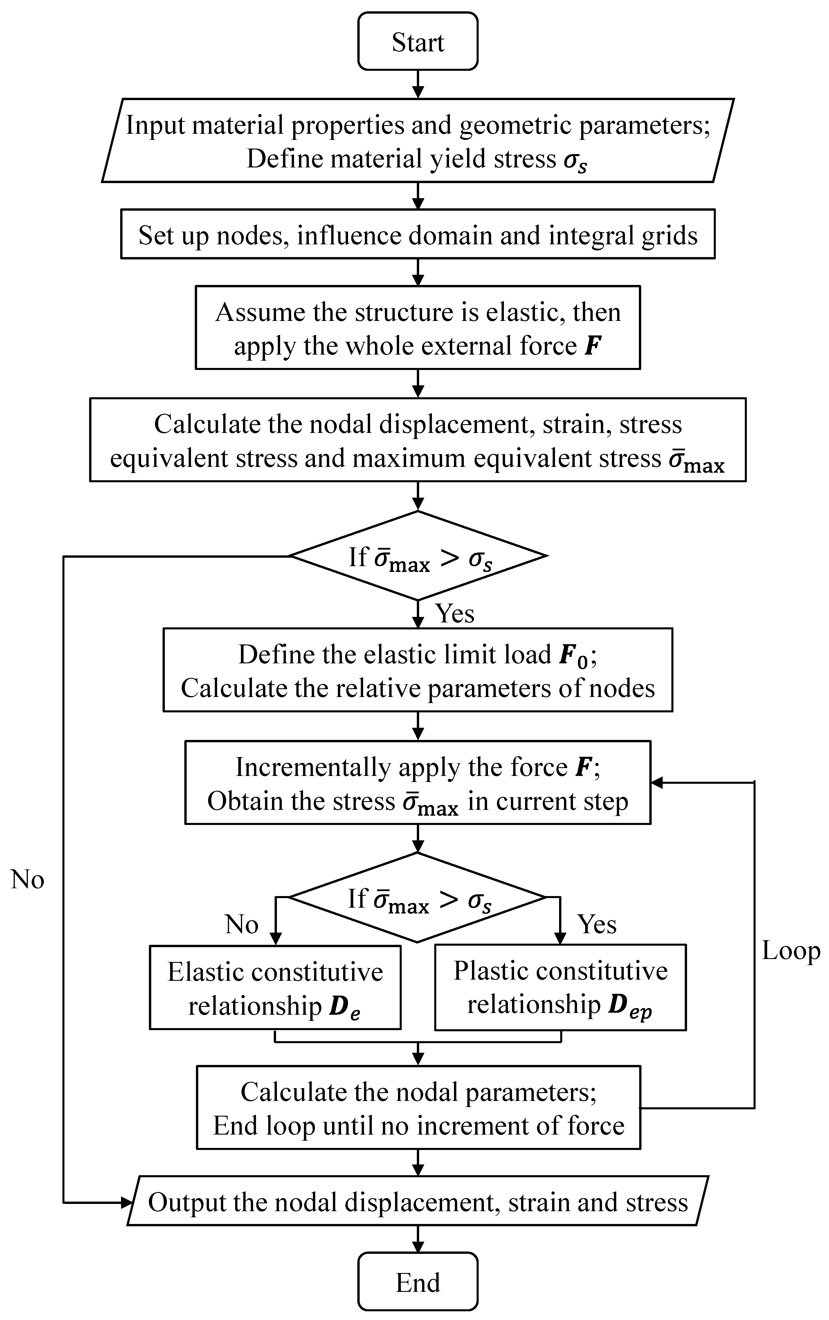
2.3. Incremental Tangent Stiffness Matrix Method

In this part, the incremental tangent stiffness matrix method is applied to solve the nonlinear Equation (36) in the plastic state, due to the nonlinearity of the constitutive relationship in Equation (6) [36,37]. In this method, the total load is divided into sufficiently small loads, which are applied step by step. Then, the nonlinear process is decomposed into a sequence of approximately linear processes.

In each approximately linear process, the relation between the stress increment tensor $\Delta \mathit{\sigma }$ and strain increment tensor $\Delta \mathit{\epsilon }$ is

$$\Delta \mathit{\sigma }={\mathit{D}}_{ep}\Delta \mathit{\epsilon },$$

(39)

which is linear, and ${\mathit{D}}_{ep}$ is only connected with the known stress and strain.

To solve this problem, first, we must determine whether the structure produces plastic deformation when applying the total external force. Under this circumstance, assume that the structure is completely in the elastic state; then the displacement, strain, stress, equivalent stress, and the maximum equivalent stress ${\overline{\sigma }}_{\max }$ of all nodes and Gauss points are obtained by using the elastic constitutive relationship in Equation (5). Denote the material yield stress as ${\sigma }_s$.

If ${\overline{\sigma }}_{\max }\le {\sigma }_s$, the structure is still in the elastic state, and the above solutions are the final solutions of this problem. If ${\overline{\sigma }}_{\max }>{\sigma }_s$, the structure has produced plastic deformation, and the external force should be applied using the incremental method. Define the elastic limit load ${\mathit{F}}_0=\frac{{\sigma }_s}{{\overline{\sigma }}_{\max }}\mathit{F}$; then the displacement, stress, and strain in the elastic state can be obtained. Behind the elastic state, we use the incremental method to apply the rest of the external force,

$$\Delta {\mathit{F}}_i=\frac{1}{N}(1-\frac{{\sigma }_s}{{\overline{\sigma }}_{\max }})\mathit{F},$$

(40)

where $N$ is the total number of load steps. In the $i-th$ load step, $\Delta {\mathit{F}}_i$ is the incremental force. Then, the solving equation is obtained,

$$\mathit{K}({\mathit{\sigma }}_{i-1})\Delta {\mathit{U}}_i=\Delta {\mathit{F}}_i,$$

(41)

where the matrix $\mathit{K}$ is related to the known stress ${\mathit{\sigma }}_{i-1}$ in the previous load step, and $\Delta {\mathit{U}}_i$ is the displacement increment in the $i-th$ load step. Then, depending on $\Delta {\mathit{U}}_i$, we can obtain the strain increment $\Delta {\mathit{\epsilon }}_i$ and the stress increment $\Delta {\mathit{\sigma }}_i$ in the current load step.

Then the stress in the $i-th$ load step can be obtained as,

$${\mathit{\sigma }}_i={\mathit{\sigma }}_{i-1}+\Delta {\mathit{\sigma }}_i.$$

(42)

In each load step, it is still necessary to choose the elastic or plastic constitutive relationship according to the relation between the stresses ${\overline{\sigma }}_{\max }$ and ${\sigma }_s$. Repeat the above process until the whole external force is applied. Eventually, the obtained displacement, stress, and strain are the final solutions of the elastic–plastic problem. The whole computing procedure is described in Figure 1.

To guarantee that the computed solutions are more accurate, in each load step the Equation (41) is modified to

$$\mathit{K}({\sigma }_{i-1})\Delta {\mathit{U}}_i={\mathit{F}}_i-{\displaystyle {\int }_{\mathsf{\Omega }}{\mathit{B}}^{\mathrm{T}}{\mathit{\sigma }}_{i-1}\mathrm{d}\mathsf{\Omega }},$$

(43)

where the second term on the right side is the equivalent node load, and ${\mathit{F}}_i$ is the total equivalent node load in the $i-th$ load step,

$${\mathit{F}}_i={\mathit{F}}_0+\Delta {\mathit{F}}_1+\Delta {\mathit{F}}_2+\cdots +\Delta {\mathit{F}}_i.$$

(44)

Based on Equation (40), the above expression can be rewritten as

$${\mathit{F}}_i=\frac{{\sigma }_s}{{\overline{\sigma }}_{\max }}\mathit{F}+\frac{i}{N}(1-\frac{{\sigma }_s}{{\overline{\sigma }}_{\max }})\mathit{F}, (i=1, 2, \dots , N).$$

(45)

3. Numerical Examples

Since there are no analytical solutions for nonlinear elastic–plastic problems, the ABAQUS program is used as a reference in this paper. In this section, to validate the numerical advantages of the IICVEFG method, three numerical examples under different constraints and forces are simulated and analysed. The solutions obtained from the IICVEFG method are compared with the solutions obtained from the ABAQUS program and the non-interpolating ICVEFG method [38].

For the following examples, the linear basis function and the $4\times 4$ Gauss points are used in the IICVEFG and ICVEFG methods. The singular weight function and cubic spline weight function are used in the IICVEFG and ICVEFG methods, respectively [23,30]. In the ABAQUS program, the C3D8R element is selected. Additionally, the external load is applied with $N=100$ steps. In this paper, two-dimensional elastic–plastic problems are regarded as plane stress problems, and the tangent modulus $E^{\prime }$ in Equation (11) is given as $E^{\prime }=0.2E$.

For error analysis, define the error between the ABAQUS program and other numerical methods, and the traditional relative error at a specific node, respectively,

$$e_i^{\mathrm{ABAQUS}}=\frac{1}{n}{\displaystyle \sum _{I=1}^n{(u_I^{\mathrm{ABAQUS}}-u_I^i)}^2},$$

(46)

$$e=\left|\frac{u_I^i-u_I^{\mathrm{ABAQUS}}}{u_I^{\mathrm{ABAQUS}}}\right|,$$

(47)

where $n$ is the number of the nodes, and i represents the IICVEFG and ICVEFG methods in this paper.

For convergence analysis, define the following variance between the different node distributions,

$$E_{ij}=\frac{1}{n}{\displaystyle \sum _{I=1}^n[{(u_I^i-u_I^{ij})}^2+{(u_I^j-u_I^{ij})}^2]},$$

(48)

where $u_I^{ij}$ represents the average displacement value of node $I$ under two different kinds of node distributions $i$ and $j$.

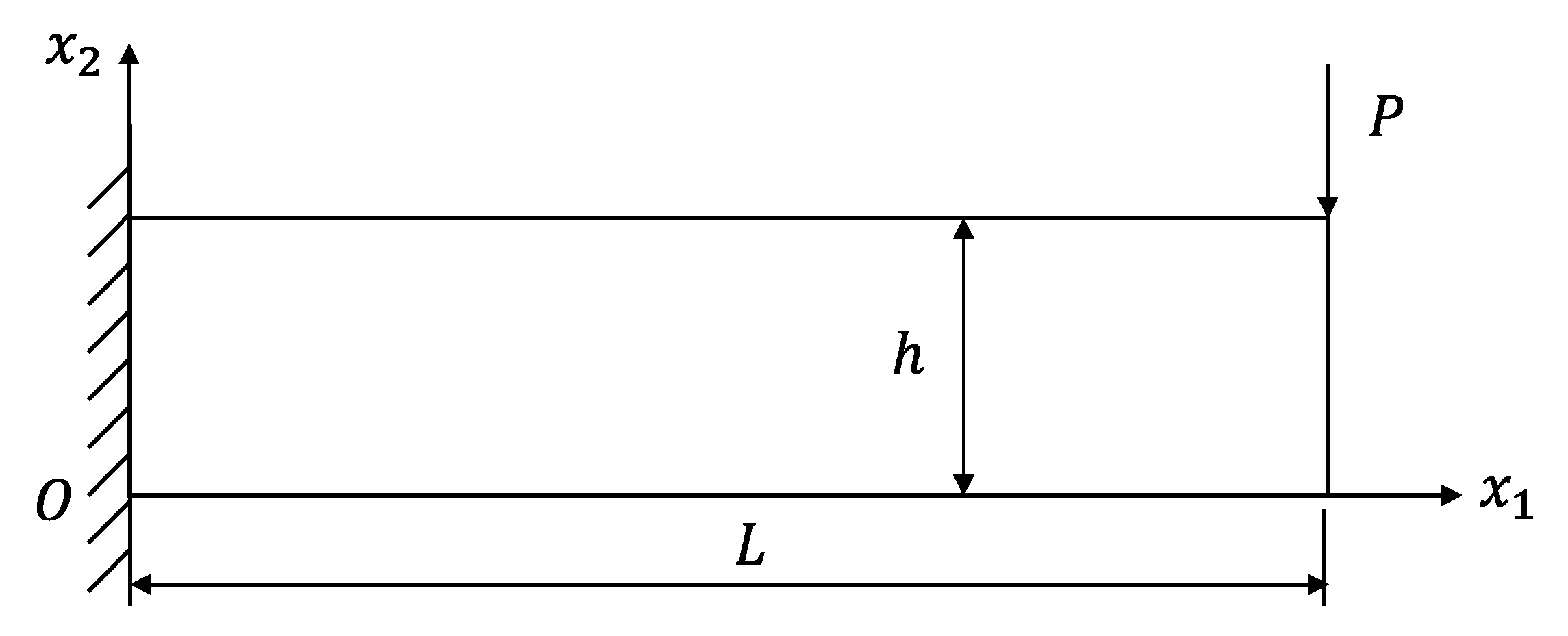
3.1. A cantilever Beam Constrained with a Concentrated Force

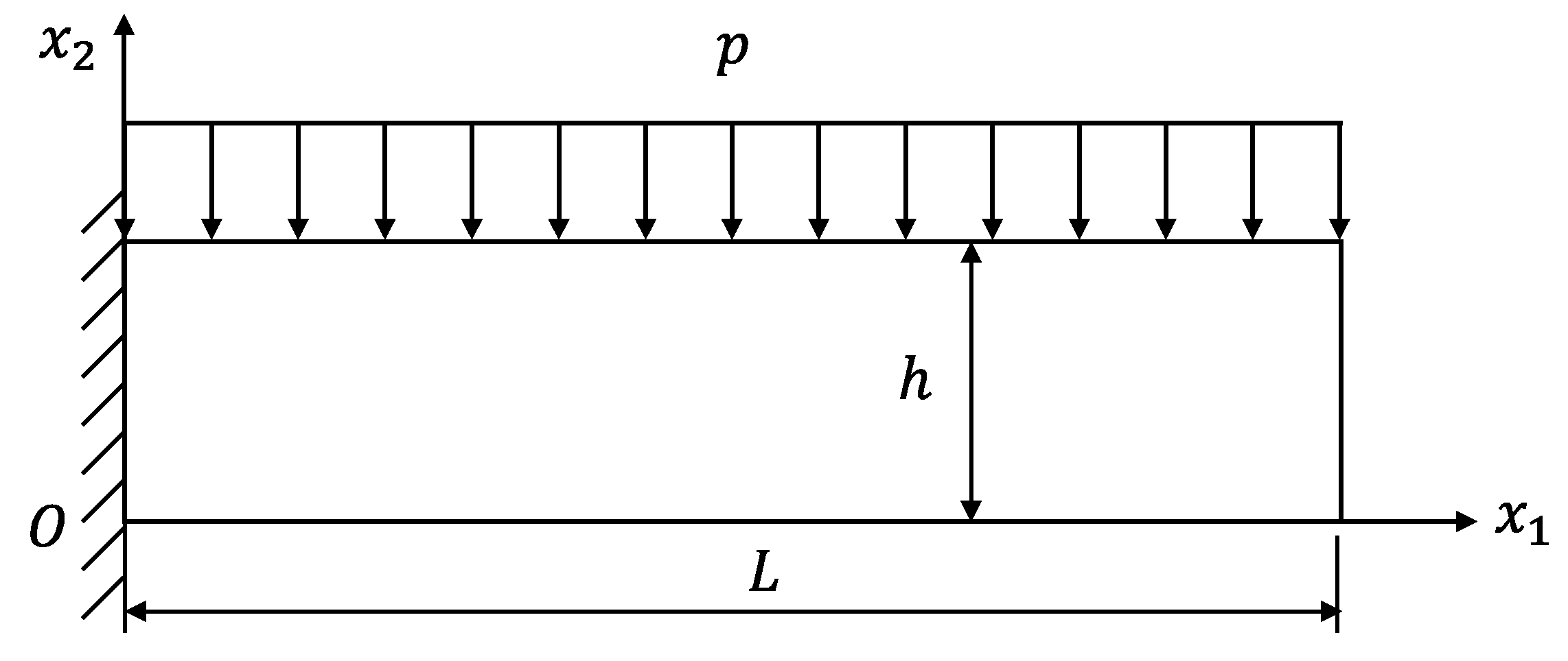
The first example is a cantilever beam; the free end is constrained with a concentrated force, as displayed in Figure 2. The geometric parameters are: $\mathit{L}=8 \mathrm{m}$, $h=1 \mathrm{m}$ and the depth is the unit length. The material parameters are: $E=1.0 \times {10}^5 \mathrm{Pa}$, $\nu =0.25$, and ${\sigma }_s=25 \mathrm{Pa}$. The concentrated load is $P=-1 \mathrm{N}$.

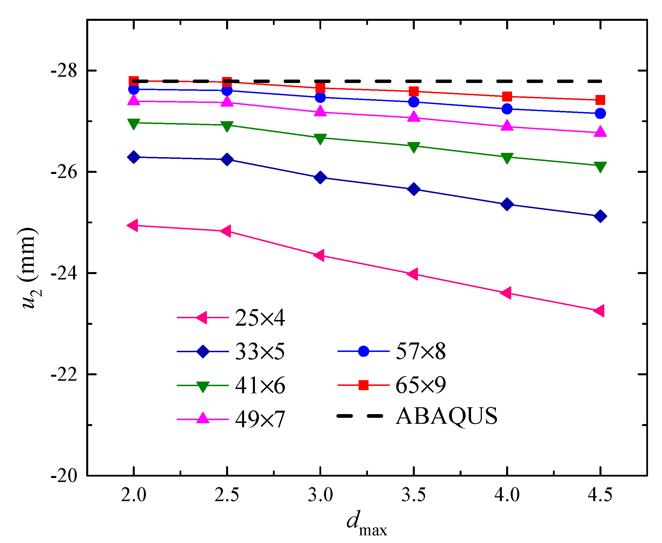
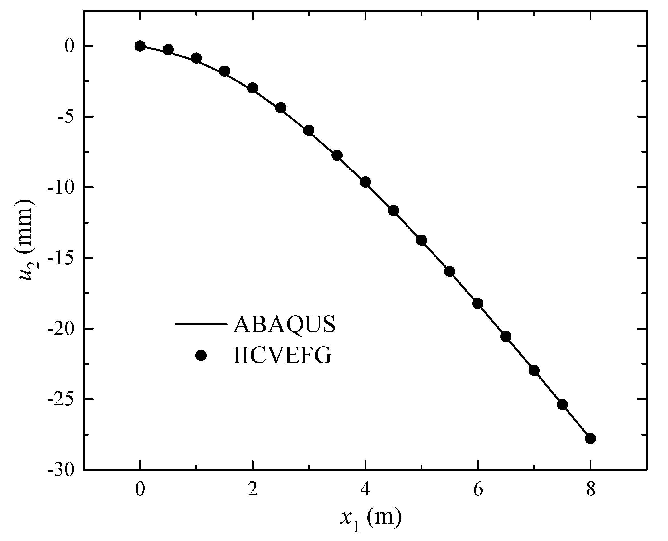
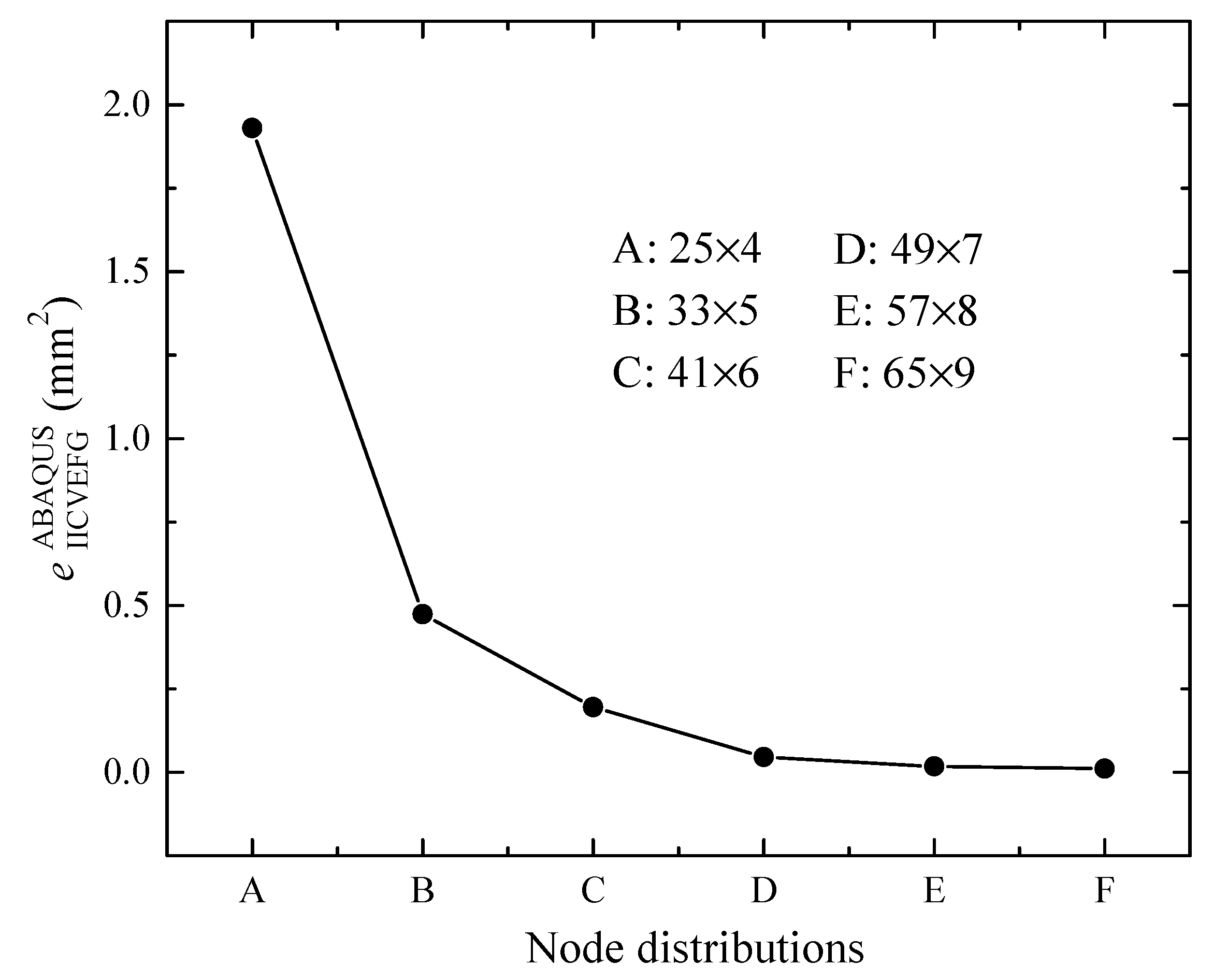
For this example, we mainly discuss the influence of the parameter scale $d_{\max }$ and different node distributions (as described in Figure 3) on the presented IICVEFG method. In the ABAQUS program, $64\times 8$ square four-node elements are. From Figure 3, it is clear that, with the decrease in the $d_{\max }$ value and the increase in the total number of nodes, the numerical solutions obtained from the IICVEFG method at point $(8, 0)$ are closer to the solutions of the ABAQUS program. From Figure 4 and the error analysis of Figure 5, we can also see that under $d_{\max }=2$ and a $65\times 9$ node distribution, the numerical deflection $u_2$ of the nodes on the $x_1$ axis of the IICVEFG method is consistent with the ABAQUS solutions.

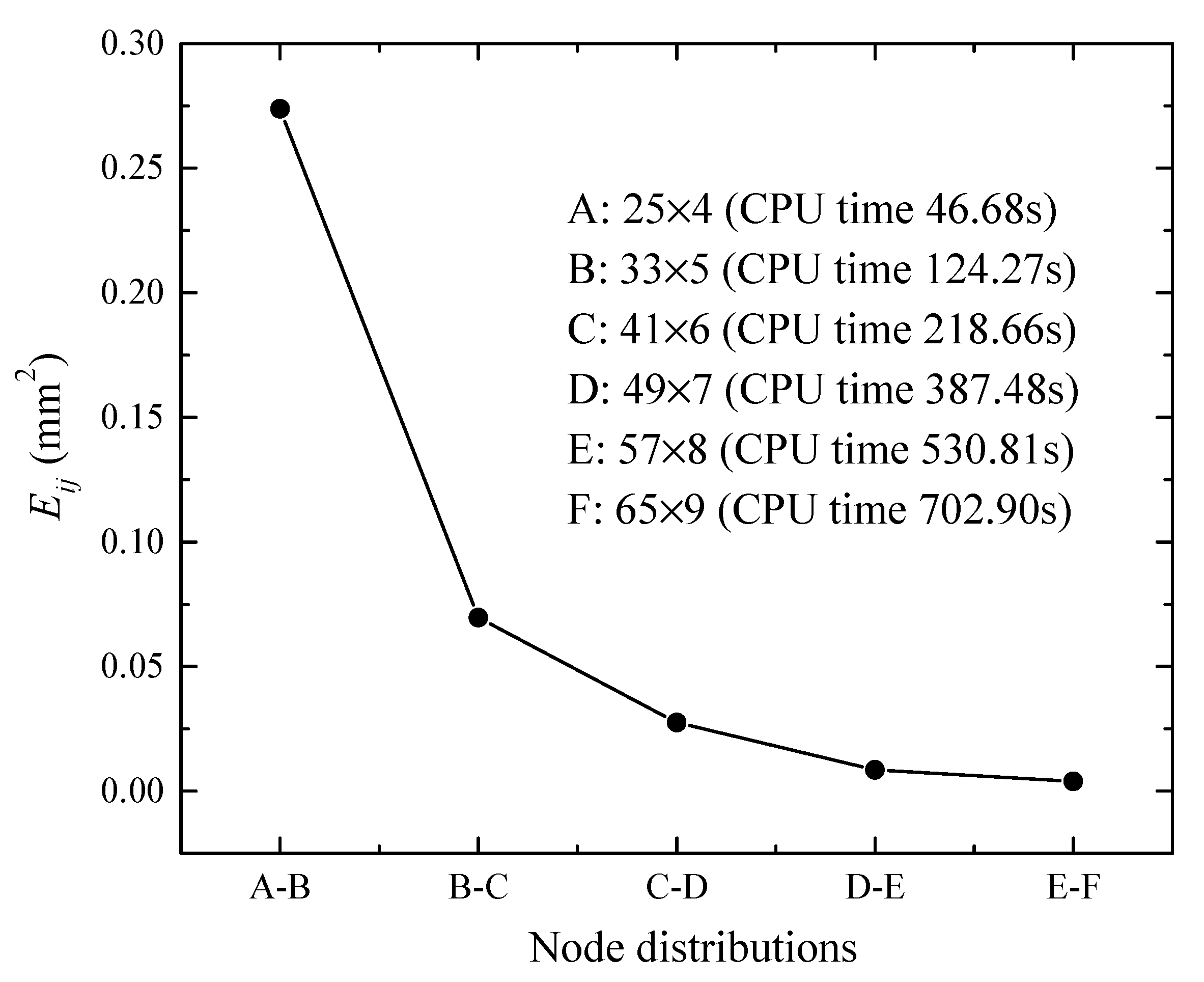
Figure 6 shows the convergence of the IICVEFG method between different node distributions. We can conclude that the greater the number of total nodes is, the smaller the variance is. Therefore, the IICVEFG method has good numerical convergence. We should note that the IICVEFG method may spend more CPU computing time as the number of total nodes increases.

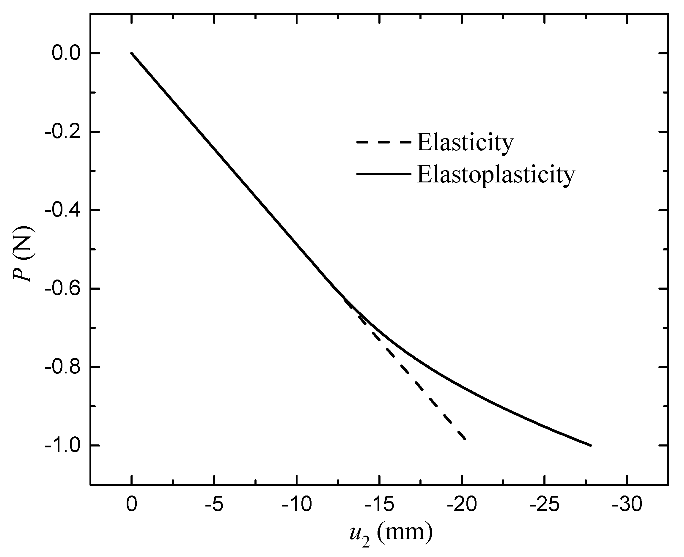
Figure 7 describes the relation between the load and the deflection $u_2$ at the point $(8, 0.5)$. When loaded to about $P=-0.6 \mathrm{N}$, the structure starts to enter plastic stage. Until about $P=-0.8 \mathrm{N}$, the whole structure is in the plastic stage.

3.2. A Cantilever Beam Constrained with a Distributed Load

The second example is a cantilever beam where the upper boundary is constrained with a distributed load, as described in Figure 8. The geometric and material parameters are the same as in the first example. The distributed load is $p=-1 \mathrm{N}/\mathrm{m}$.

For this example, we mainly discuss the merits of the IICVEFG method in terms of computing accuracy and efficiency, as compared to the non-interpolating ICVEFG method. In the IICVEFG method, $17\times 4$ nodes are used. The grid distribution in the ABAQUS program is same as the first example.

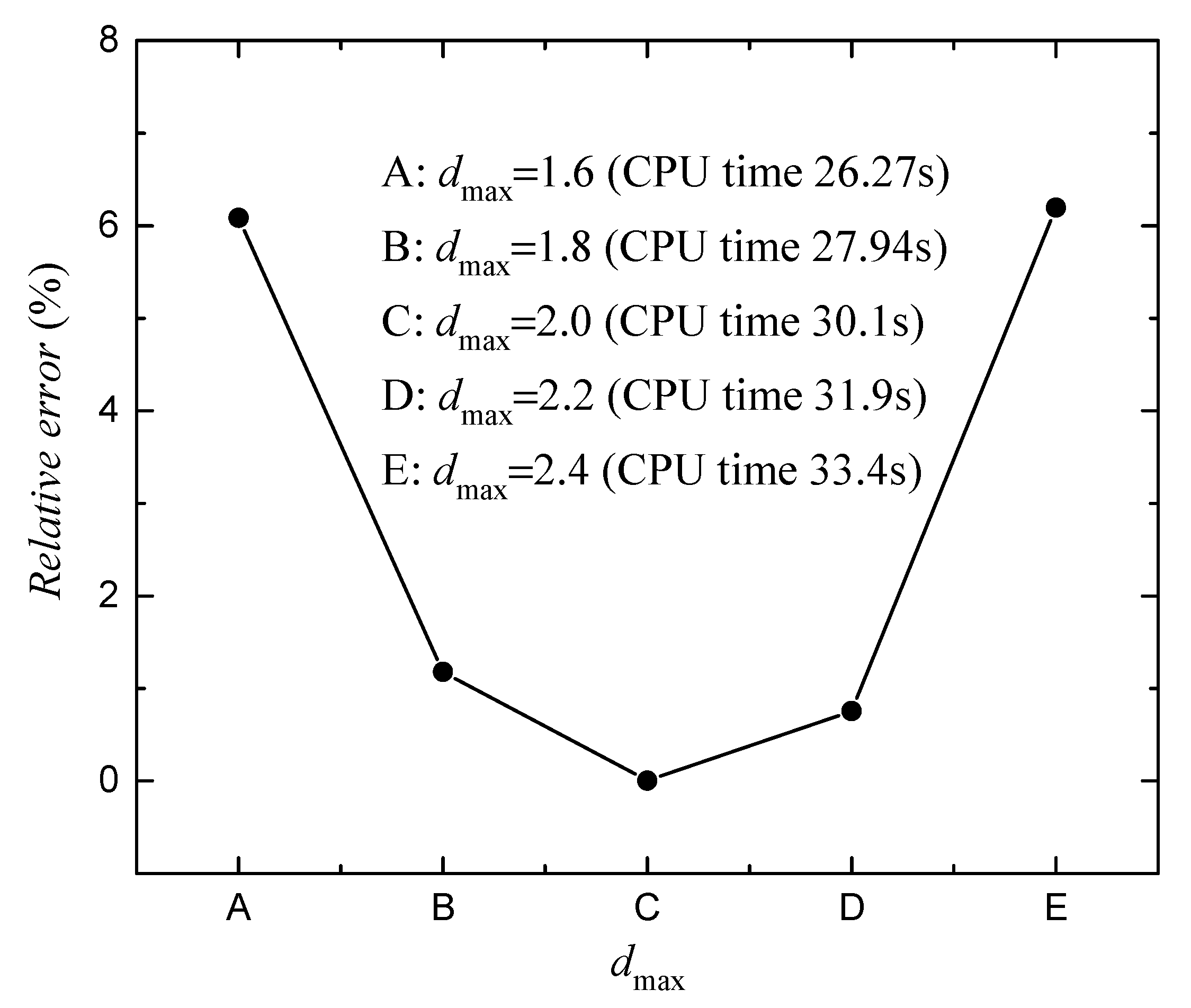
Under different parameter scalings $d_{\max }$, Figure 9 shows the relative errors of the deflection $u_2$ at point $(8, 0)$ between the IICVEFG method and ABAQUS program. It is clear that when $d_{\max }=2$, the relative error is close to zero. Thus, we choose these data for the following discussion. It widely known that the greater the value of $d_{\max }$ is, the more CPU time the IICVEFG method requires.

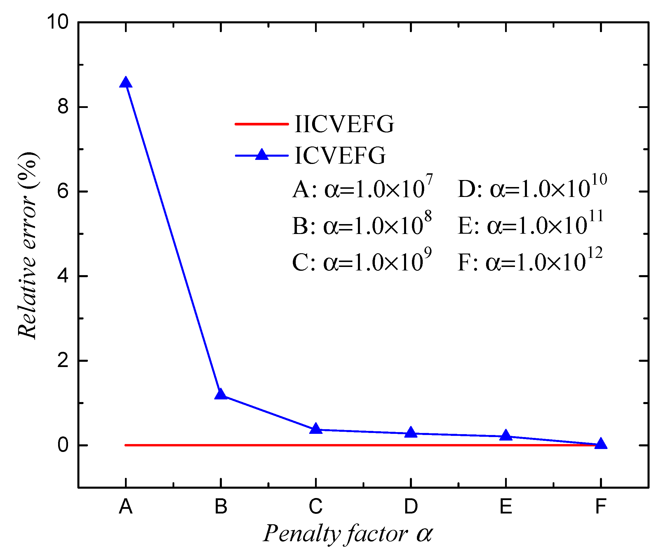
Taking the ICVEFG method as a comparison method, the suitable node distribution, $d_{\max }$, and penalty factor $\alpha$ should be chosen. For this example, $21\times 11$ nodes and $d_{\max }=3.9$ are used. The penalty factor $\alpha$ is chosen according to Figure 10. From the relative error analysis, there are two observations: (1) The solutions of the IICVEFG method have no relation with the penalty factor $\alpha$, because in the IICVEFG method special techniques are unnecessary when applying the essential boundary conditions; (2) With the increase in the penalty factor $\alpha$ the relative error is gradually reduced, and when $\alpha =1.0\times {10}^{12}$ the relative error is sufficiently small and close to the error of the IICVEFG method. It is worth mentioning that this selection process is time consuming. Therefore, the IICVEFG method has a greater computing accuracy and efficiency than the ICVEFG method.

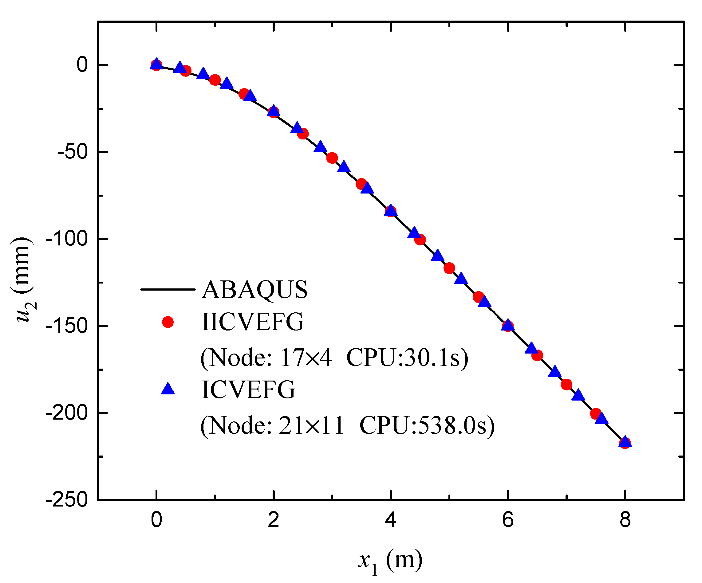
After deciding the values of the relative parameters, the deflection $u_2$ of the nodes on the $x_1$ axis are acquired from the ABAQUS program, as well as the IICVEFG and ICVEFG methods. The results are shown in Figure 11. The solutions are in good agreement with each other. Moreover, for a single calculation, the CPU time spent in the IICVEFG method is $30.1 \mathrm{s}$, which is much less than the $538.0 \mathrm{s}$ spent in the ICVEFG method under similar accuracy.

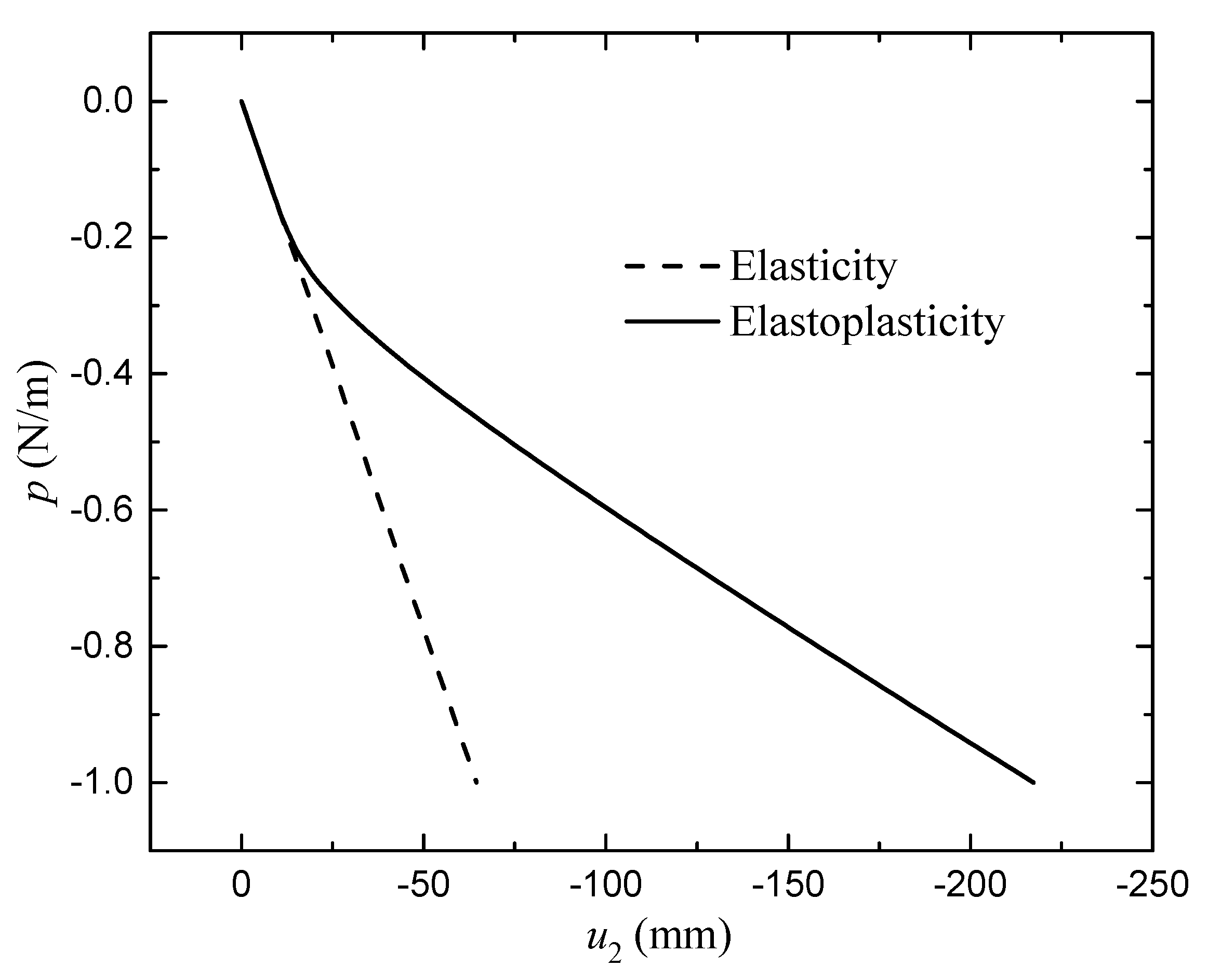
Identically to the first example, the relation between the load and the deflection $u_2$ at the point $(8, 0)$ is shown in Figure 12. For this example, the structure begins to produce the plastic deformation when $p=-0.2 \mathrm{N}/\mathrm{m}$, and up to $p=-0.4 \mathrm{N}/\mathrm{m}$ the structure is completely in the plastic stage.

3.3. A Rectangular Plate with a Central Hole under a Distributed Traction

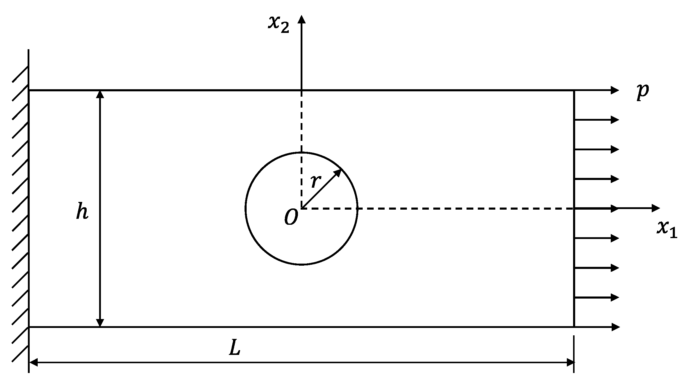
The final example is a rectangular plate with a circular hole in the centre. This structure bears a distributed traction at the right boundary, as described in Figure 13. The geometric parameters are: $\mathit{L}=10 \mathrm{m}$, $h=4 \mathrm{m}$, $r=1 \mathrm{m}$, and the depth is the unit length. The material parameters are: $E=1.0\times {10}^5 \mathrm{Pa}$, $\nu =0.25$, and ${\sigma }_s=250 \mathrm{Pa}$. The traction load is $p=1000 \mathrm{N}/\mathrm{m}$.

For this example, we mainly discuss the applicability of the IICVEFG model for complex structures. First, for the IICVEFG and ICVEFG methods, the numerical solutions were obtained under the same node distribution $23\times 15$. In the IICVEFG and ICVEFG methods $d_{\max }=2$. Moreover, in the ICVEFG method $\alpha =1.0\times {10}^9$. As a reference, $40\times 8$ grids are distributed in the ABAQUS program.

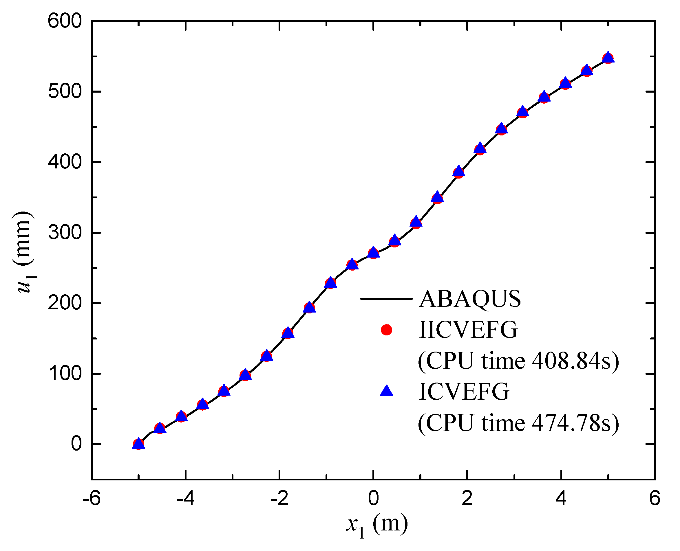
Figure 14 shows the displacement $u_1$ of the nodes on $x_2=-2 \mathrm{m}$. We can see that the solutions obtained from the IICVEFG and ICVEFG methods are in good agreement with the solutions of the ABAQUS program. The relative errors at point $(5, -2)$ acquired from the IICVEFG and ICVEFG methods are $0.144\%$ and $0.1611\%$, respectively. Furthermore, under similar computing accuracy, the IICVEFG method requires $408.84 \mathrm{s}$ to compute, which is less than the $474.78 \mathrm{s}$ for the ICVEFG method.

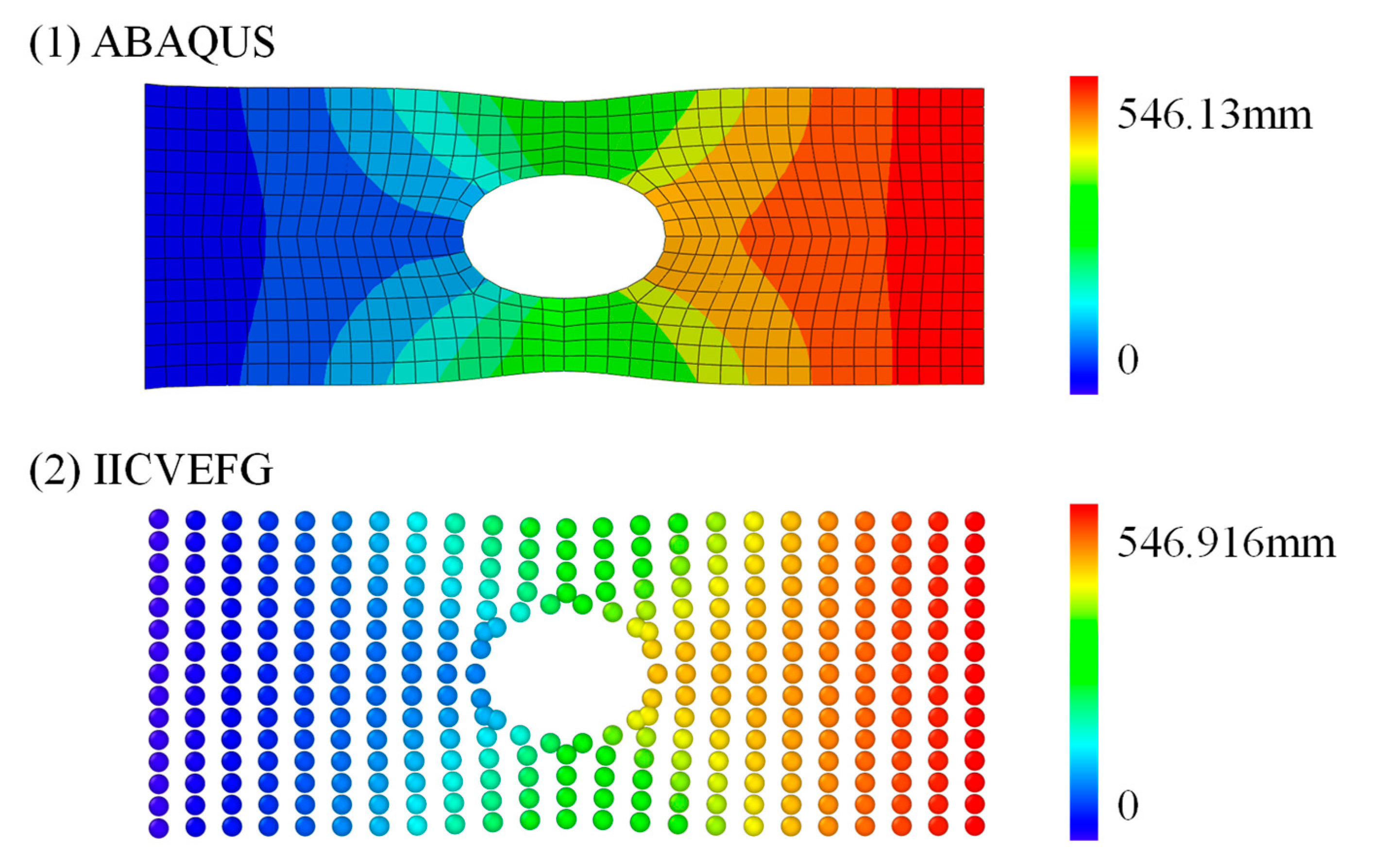
Figure 15 describes the grid distribution in the ABAQUS program, node distribution in the IICVEFG method, and the corresponding distributions of displacement $u_1$. We can see that the displacement distributions obtained from the ABAQUS program and IICVEFG method are similar.

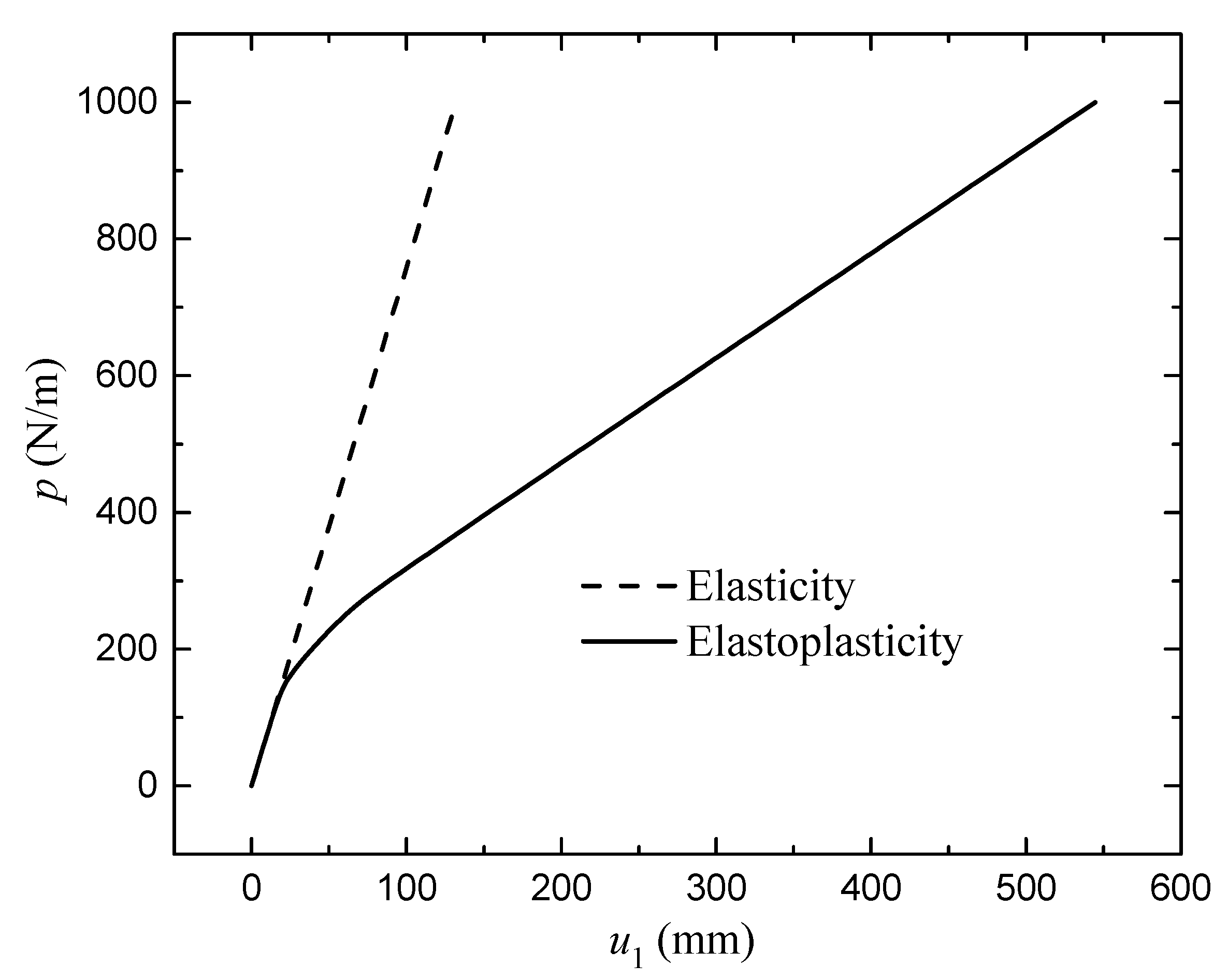
For this example, the relation of the traction and the displacement $u_1$ at point $(5, 0)$ is also discussed in Figure 16. Around the value $p=100 \mathrm{N}/\mathrm{m}$ the plastic deformation occurs; and around $p=300 \mathrm{N}/\mathrm{m}$ the deformation of the whole structure is plastic deformation.

4. Conclusions

In this paper, a more efficient and accurate numerical model for the two-dimensional nonlinear elastic–plastic problems is established, based on the IICVEFG method and the incremental tangent stiffness matrix method. Through numerical analyses we found that, in the IICVEFG method, the variance is smaller as the number of total nodes increases. Thus, the IICVEFG method has good convergence. The solutions of the IICVEFG method are consistent with the solutions of the ABAQUS program. In addition, the error between the IICVEFG method and ABAQUS program is less than that between the ICVEFG method and ABAQUS program. Furthermore, under similar accuracy constraints, the CPU time spent on the IICVEFG method is $30.1 \mathrm{s}$, which is much less than $538.0 \mathrm{s}$ spent on the ICVEFG method. Thus, the IICVEFG method has greater numerical accuracy and efficiency than the non-interpolating ICVEFG method for different elastic–plastic problems. This validates that the IICVEFG method is sufficiently adaptable.

References

- Mcmeeking, R.M.; Rice, J.R. Finite-element formulations for problems of large elastic-plastic deformation. Int. J. Solids Struct. 1975, 11, 601–616. [Google Scholar] [CrossRef] [Green Version]
- Barry, W.; Saigal, S. A three-dimensional element-free Galerkin elastic and elastoplastic formulation. Int. J. Numer. Meth. Eng. 1999, 46, 671–693. [Google Scholar] [CrossRef]
- Schreyer, H.L.; Kulak, R.F.; Kramer, J.M. Accurate Numerical Solutions for Elastic-Plastic Models. J. Press. Vess-T 1979, 101, 226–234. [Google Scholar] [CrossRef]
- Rong, B.; Rui, X.T.; Tao, T.; Wang, G.P. Theoretical modeling and numerical solution methods for flexible multibody system dynamics. Nonlinear Dyn. 2019, 98, 1519–1553. [Google Scholar] [CrossRef]
- Ostiguy, G.L.; Sassi, S. Effects of initial geometric imperfections on dynamic behavior of rectangular plates. Nonlinear Dyn. 1992, 3, 165–181. [Google Scholar] [CrossRef]
- Mahdiabadi, M.K.; Tiso, P.; Brandt, A.; Rixen, D.J. A non-intrusive model-order reduction of geometrically nonlinear structural dynamics using modal derivatives. Mech. Syst. Signal Process. 2021, 147, 107126. [Google Scholar] [CrossRef]
- Vaiana, N.; Losanno, D.; Ravichandran, N. A novel family of multiple springs models suitable for biaxial rate-independent hysteretic behavior. Comput. Struct. 2021, 244, 106403. [Google Scholar] [CrossRef]
- Vaiana, N.; Sessa, S.; Rosati, L. A generalized class of uniaxial rate-independent models for simulating asymmetric mechanical hysteresis phenomena. Mech. Syst. Signal Process. 2021, 146, 106984. [Google Scholar] [CrossRef]
- Vaiana, N.; Sessa, S.; Paradiso, M.; Rosati, L. Accurate and efficient modeling of the hysteretic behavior of sliding bearings. In Proceedings of the 7th International Conference on Computational Methods in Structural Dynamics and Earthquake Engineering Methods in Structural Dynamics and Earthquake Engineering, Crete, Greece, 24–26 June 2019. [Google Scholar]
- Belytschko, T.; Lu, Y.Y.; Gu, L. Element-free Galerkin methods. Int. J. Numer. Meth. Eng. 1994, 37, 229–256. [Google Scholar] [CrossRef]
- Belytschko, T.; Krongauz, Y.; Organ, D.; Fleming, M.; Krysl, P. Meshless methods: An overview and recent development. Comput. Methods Appl. Mech. Eng. 1996, 139, 3–47. [Google Scholar] [CrossRef] [Green Version]
- Chen, J.S.; Pan, C.; Wu, C.T.; Liu, W.K. Reproducing kernel particle methods for large deformation analysis of non-linear structures. Comput. Methods Appl. Mech. 1996, 139, 195–227. [Google Scholar] [CrossRef]
- Cheng, Y.M.; Bai, F.N.; Liu, C.; Peng, M.J. Analyzing nonlinear large deformation with an improved element-free Galerkin method via the interpolating moving least-squares method. Int. J. Comput. Mater. Sci. Eng. 2016, 5, 1650023. [Google Scholar] [CrossRef]
- Fleming, M.; Chu, Y.A.; Moran, B.; Belytschko, T. Enriched element-free Galerkin methods for crack tip fields. Int. J. Numer. Meth. Eng. 1997, 40, 1483–1504. [Google Scholar] [CrossRef]
- Memari, A.; Mohebalizadeh, H. Quasi-static analysis of mixed-mode crack propagation using the meshless local Petrov-Galerkin method. Eng. Anal. Bound. Elem. 2019, 106, 397–411. [Google Scholar] [CrossRef]
- Jiang, F.; Oliveira, M.S.A.; Sousa, A.C.M. Mesoscale SPH modeling of fluid flow in isotropic porous media. Comput. Phys. Commun. 2007, 176, 471–480. [Google Scholar] [CrossRef]
- Moradi, D.R.; Radhi, A.; Behdinan, K. Damped dynamic behavior of an advanced piezoelectric sandwich plate. Compos. Struct. 2020, 243, 112243. [Google Scholar] [CrossRef]
- Liu, M.B.; Liu, G.R. Smoothed particle hydrodynamics (SPH): An overview and recent developments. Arch. Comput. Methods Eng. 2010, 17, 25–76. [Google Scholar] [CrossRef] [Green Version]
- Liu, W.K.; Chen, Y.; Jun, S.; Chen, J.S.; Belytschko, T.; Pan, C.; Uras, R.A.; Cheng, C.T. Overview and applications of the reproducing kernel particle methods. Arch. Comput. Methods Eng. 1996, 3, 3–80. [Google Scholar] [CrossRef]
- Peng, M.J.; Li, D.M.; Cheng, Y.M. The complex variable element-free Galerkin (CVEFG) method for elasto-plasticity problems. Eng. Struct. 2011, 33, 127–135. [Google Scholar] [CrossRef]
- Liew, K.M.; Feng, C.; Cheng, Y.M.; Kitipornchai, S. Complex variable moving least-squares method: A meshless approximation technique. Int. J. Numer. Meth. Eng. 2007, 70, 46–70. [Google Scholar] [CrossRef]
- Cheng, Y.M.; Li, J.H. Complex variable meshless method for fracture problems. Sci. China Ser. G 2006, 49, 46–59. [Google Scholar] [CrossRef]
- Bai, F.N.; Li, D.M.; Wang, J.F.; Cheng, Y.M. An improved complex variable element-free Galerkin method for two-dimensional elasticity problems. Chin. Phys. B 2012, 21, 020204. [Google Scholar] [CrossRef]
- Li, D.M.; Liew, K.M.; Cheng, Y.M. An improved complex variable element-free Galerkin method for two-dimensional large deformation elastoplasticity problems. Comput. Methods Appl. Mech. 2014, 269, 72–86. [Google Scholar] [CrossRef]
- Zhang, L.W.; Deng, Y.J.; Liew, K.M. An improved element-free Galerkin method for numerical modeling of the biological population problems. Eng. Anal. Bound. Elem. 2014, 40, 181–188. [Google Scholar] [CrossRef]
- Wang, J.F.; Sun, F.X.; Cheng, Y.M. An improved interpolating element-free Galerkin method with nonsingular weight function for two-dimensional potential problems. Chin. Phys. B 2012, 21, 090204. [Google Scholar] [CrossRef]
- Sun, F.X.; Wang, J.F.; Cheng, Y.M.; Huang, A.X. Error estimates for the interpolating moving least-squares method in n-dimensional space. Appl. Numer. Math. 2015, 98, 79–105. [Google Scholar] [CrossRef]
- Ren, H.P.; Cheng, Y.M. The interpolating element-free Galerkin (IEFG) method for two-dimensional elasticity problems. Int. J. Appl. Mech. 2011, 3, 735–758. [Google Scholar] [CrossRef]
- Deng, Y.J.; Liu, C.; Peng, M.J.; Cheng, Y.M. The interpolating complex variable element-free Galerkin method for temperature field problems. Int. J. Appl. Mech. 2015, 7, 1550017. [Google Scholar] [CrossRef]
- Deng, Y.J.; He, X.Q. An improved interpolating complex variable meshless method for bending problem of Kirchhoff plates. Int. J. Appl. Mech. 2017, 9, 1750089. [Google Scholar] [CrossRef]
- Ren, H.P.; Cheng, J.; Huang, A.X. The complex variable interpolating moving least-squares method. Appl. Math. Comput. 2012, 219, 1724–1736. [Google Scholar] [CrossRef]
- Deng, Y.J.; He, X.Q.; Dai, Y. The improved interpolating complex variable element free Galerkin method for two-dimensional potential problems. Int. J. Appl. Mech. 2019, 11, 1950104. [Google Scholar] [CrossRef]
- Deng, Y.J.; He, X.Q.; Sun, L.G.; Yi, S.H.; Dai, Y. An improved interpolating complex variable element free Galerkin method for the pattern transformation of hydrogel. Eng. Anal. Bound. Elem. 2020, 113, 99–109. [Google Scholar] [CrossRef]
- Yu, S.Y.; Peng, M.J.; Cheng, H.; Cheng, Y.M. The improved element-free Galerkin method for three-dimensional elastoplasticity problems. Eng. Anal. Bound. Elem. 2019, 104, 215–224. [Google Scholar] [CrossRef]
- Cheng, Y.M. Meshless Methods; Science Press: Beijing, China, 2015. [Google Scholar]
- Cheng, Y.M.; Bai, F.N.; Peng, M.J. A novel interpolating element-free Galerkin (IEFG) method for two-dimensional elastoplasticity. Appl. Math. Model. 2014, 38, 5187–5197. [Google Scholar] [CrossRef]
- Sun, F.X.; Wang, J.F.; Cheng, Y.M. An improved interpolating element-free Galerkin method for elastoplasticity via nonsingular weight functions. Int. J. Appl. Mech. 2016, 8, 1650096. [Google Scholar] [CrossRef]
- Cheng, Y.M.; Wang, J.F.; Bai, F.N. A new complex variable element-free Galerkin method for two-dimensional potential problems. Chin. Phys. B. 2012, 21, 090203. [Google Scholar] [CrossRef]
Figure 1.
Flow chart of the computing procedure.
Figure 2.
Cantilever beam constrained with a concentrated force.
Figure 3.
The influence of and node distributions on the IICVEFG method.
Figure 4.
The deflection of the nodes on the axis.
Figure 5.
The error analysis under different node distributions.
Figure 6.
The convergence analysis and CPU time.
Figure 7.
The relation between the load and the deflection.
Figure 8.
Cantilever beam constrained with a distributed load.
Figure 9.
The relative errors and CPU time under different .
Figure 10.
The influence of penalty factor .
Figure 11.
Figure 12.
Figure 13.
Rectangular plate with a central hole under a distributed traction.
Figure 14.
The displacement of the nodes on .
Figure 15.
The displacement distributions.
Figure 16.
The relation between the displacement and traction.
Publisher’s Note: MDPI stays neutral with regard to jurisdictional claims in published maps and institutional affiliations. |
© 2021 by the authors. Licensee MDPI, Basel, Switzerland. This article is an open access article distributed under the terms and conditions of the Creative Commons Attribution (CC BY) license (https://creativecommons.org/licenses/by/4.0/).
Share and Cite
MDPI and ACS Style
Deng, Y.; Shen, X.; Tao, J.; Dai, Y. Analysis of Elastic–Plastic Problems Using the Improved Interpolating Complex Variable Element Free Galerkin Method. Mathematics 2021, 9, 1967. https://doi.org/10.3390/math9161967
AMA Style
Deng Y, Shen X, Tao J, Dai Y. Analysis of Elastic–Plastic Problems Using the Improved Interpolating Complex Variable Element Free Galerkin Method. Mathematics. 2021; 9(16):1967. https://doi.org/10.3390/math9161967
Chicago/Turabian StyleDeng, Yajie, Xingkeng Shen, Jixiao Tao, and Ying Dai. 2021. "Analysis of Elastic–Plastic Problems Using the Improved Interpolating Complex Variable Element Free Galerkin Method" Mathematics 9, no. 16: 1967. https://doi.org/10.3390/math9161967
Note that from the first issue of 2016, this journal uses article numbers instead of page numbers. See further details here.