
A Comprehensive Analysis of Demand Response Pricing Strategies in a Smart Grid Environment Using Particle Swarm Optimization and the Strawberry Optimization Algorithm

 ,
,  ,
,  ,
,  ,
,  and
and 
Abstract
:1. Introduction
- The pricing adopted based on the RTP location is less fair than the purchase history pricing;
- The impact towards the increase in controllable devices, selection of the DP methodology and optimization techniques is not contributed;
- Techno-economic analysis considering different load scenarios and different DP strategies is not focused. Comparative analysis of the PAR based on DP and optimization is not projected.
- Analysis of the DP schemes of DR such as TOU and RTP for industrial, commercial, and residential load scenarios is formulated.
- A techno-economic comparative analysis of PSO and the strawberry (SBY) optimization algorithm for solving the DP strategies with 109, 1992, and 7807 controllable industrial, commercial, and residential loads is performed.
- An RTP algorithm is considered using both distributed and centralized algorithms.
- A comparative analysis of the peak-to-average ratio (PAR) calculated for all load conditions with both PSO and the SBY optimization algorithm using the TOU and RTP strategies is performed.
2. Pricing Algorithms
2.1. Time-of-Use Pricing
2.2. Real-Time Pricing
3. Formulation of the RTP Load Scheduling Problem
3.1. Tentative Scheduling
3.2. Power Allocation
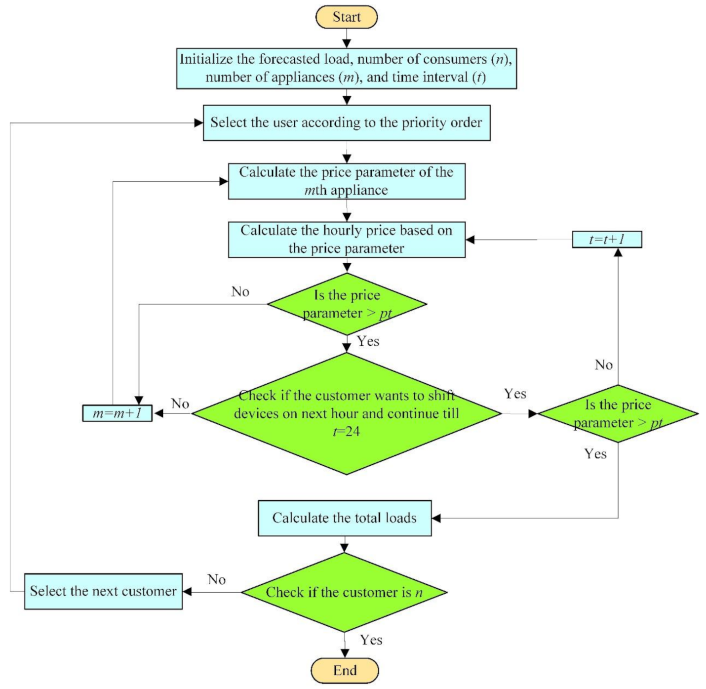
3.3. Distributed Scheduling Algorithm
- →
- Begin;
- →
- Set the value of t = 0;
- →
- At time t the device i ∈ St prepares to enter the operating mode;
- →
- For each device i calculate the pricing threshold value (Zi);
- →
- Check if Zi is lower than the RTP at t;
- →
- Check the power constraint;
- →
- If the available power is greater than the power consumed by the device (gi), run the device in that hour t, otherwise proceed to step 5;
- →
- Increment t and go to step 2. Perform until t = 24.
3.4. Centralized Scheduling Algorithm
- -
- Initialize the timeslot t = 0;
- -
- At any time t, the appliance i ∈ St is made to run;
- -
- For each appliance i in a smart home, the threshold Zi is calculated, and a signal is sent to the home energy controller (HEC);
- -
- Check for the current electricity price (t) set by the HEC. Then, select the delayed appliances whose is lower than P(t) and list them in queue ;
- -
- Solve the load-shifting problem to select the devices which can get connected and list them in queue ; the leftover appliances in should wait for the next available timeslot;
- -
- Run all the appliances waiting in the queue;
- -
- Increment t = t + 1 and go to step 2; continue till t = 24.
3.5. Peak-to-Average Ratio (PAR)
4. Optimization Algorithms
4.1. Particle Swarm Optimization (PSO)
4.2. Strawberry Optimization Algorithm (SBY)
- Select the number of mother plants (e.g., N), the number of roots (Nroot), and the number of runners (Nrunner) so that Nrunner >> Nroot. Set a group for the number of devices. The combination of devices is considered as a variable. Consider the best pattern after running the permutation for the set of devices in the group; for the best pattern of devices, run the strawberry optimization algorithm. The grouping of controllable devices is considered as the mother plant in this DR problem.
- Set the number of mother plants in the search space, as well as the iteration count.
- Randomly generate two points, the roots and the runners for every mother plant (2N points). The possible allocation of the devices in the group will be obtained as 2N vectors.
- Evaluate fitness (function to be optimized, e.g., fitness (x(i)) for every mother plant.
- Using the roulette wheel, the best N/2 fitness out of the 2N vectors is selected, as well as the elite selection selects the best N/2 fitness. The total of N best solutions from the obtained 2N fitness value is selected. The left-out N values are eliminated. The best N value takes part in the next iteration.
- Repeat steps 3–5 until the termination condition is satisfied.
4.3. System Input Data
5. Techno-Economic Analysis
6. Results and Discussion
7. Conclusions
Author Contributions
Funding
Institutional Review Board Statement
Informed Consent Statement
Data Availability Statement
Acknowledgments
Conflicts of Interest
References
- Ismael, S.M.; Abdel Aleem, S.H.E.; Abdelaziz, A.Y.; Zobaa, A.F. State-of-the-art of hosting capacity in modern power systems with distributed generation. Renew. Energy 2019, 130, 1002–1020. [Google Scholar] [CrossRef]
- Nardelli, P.; Hussain, H.M.; Narayanan, A.; Yang, Y. Virtual Microgrid Management via Software-Defined Energy Network for Electricity Sharing: Benefits and Challenges. IEEE Syst. Man Cybern. Mag. 2021, 7, 10–19. [Google Scholar] [CrossRef]
- Omar, A.I.; Ali, Z.M.; Al-Gabalawy, M.; Abdel Aleem, S.H.E.; Al-Dhaifallah, M. Multi-objective environmental economic dispatch of an electricity system considering integrated natural gas units and variable renewable energy sources. Mathematics 2020, 8, 1100. [Google Scholar] [CrossRef]
- Sakar, S.; Balci, M.E.; Abdel Aleem, S.H.E.; Zobaa, A.F. Increasing PV hosting capacity in distorted distribution systems using passive harmonic filtering. Electr. Power Syst. Res. 2017, 148, 74–86. [Google Scholar] [CrossRef] [Green Version]
- Ali, S.; Khan, I.; Jan, S.; Hafeez, G. An Optimization Based Power Usage Scheduling Strategy Using Photovoltaic-Battery System for Demand-Side Management in Smart Grid. Energies 2021, 14, 2201. [Google Scholar] [CrossRef]
- Sarker, E.; Halder, P.; Seyedmahmoudian, M.; Jamei, E.; Horan, B.; Mekhilef, S.; Stojcevski, A. Progress on the demand side management in smart grid and optimization approaches. Int. J. Energy Res. 2021, 45, 36–64. [Google Scholar] [CrossRef]
- Khan, H.N.; Iftikhar, H.; Asif, S.; Maroof, R.; Ambreen, K.; Javaid, N. Demand Side Management Using Strawberry Algorithm and Bacterial Foraging Optimization Algorithm in Smart Grid BT—Advances in Network-Based Information Systems; Barolli, L., Enokido, T., Takizawa, M., Eds.; Springer International Publishing: Cham, Switzerland, 2018; pp. 191–202. [Google Scholar]
- Scarabaggio, P.; Grammatico, S.; Carli, R.; Dotoli, M. Distributed Demand Side Management with Stochastic Wind Power Forecasting. IEEE Trans. Control Syst. Technol. 2021, 1–16. [Google Scholar] [CrossRef]
- Aoun, A.; Ghandour, M.; Ilinca, A.; Ibrahim, H. Demand-Side Management. In Hybrid Renewable Energy Systems and Microgrids; Kabalci, E., Ed.; Academic Press: Cambridge, MA, USA, 2021; pp. 463–490. ISBN 978-0-12-821724-5. [Google Scholar]
- Zeeshan, M.; Jamil, M. Adaptive Moth Flame Optimization based Load Shifting Technique for Demand Side Management in Smart Grid. IETE J. Res. 2021, 1–12. [Google Scholar] [CrossRef]
- Mariano-Hernández, D.; Hernández-Callejo, L.; Zorita-Lamadrid, A.; Duque-Pérez, O.; Santos García, F. A review of strategies for building energy management system: Model predictive control, demand side management, optimization, and fault detect & diagnosis. J. Build. Eng. 2021, 33, 101692. [Google Scholar] [CrossRef]
- Koul, B.; Singh, K.; Brar, Y.S. An introduction to smart grid and demand-side management with its integration with renewable energy. In Advances in Smart Grid Power System; Tomar, A., Kandari, R., Eds.; Academic Press: Cambridge, MA, USA, 2021; pp. 73–101. ISBN 978-0-12-824337-4. [Google Scholar]
- Salameh, K.; Awad, M.; Makarfi, A.; Jallad, A.H.; Chbeir, R. Demand side management for smart houses: A survey. Sustainability 2021, 13, 6768. [Google Scholar] [CrossRef]
- Dranka, G.G.; Ferreira, P.; Vaz, A.I.F. Integrating supply and demand-side management in renewable-based energy systems. Energy 2021, 232, 120978. [Google Scholar] [CrossRef]
- Rawa, M.; Abusorrah, A.; Bassi, H.; Mekhilef, S.; Ali, Z.M.; Abdel Aleem, S.H.E.; Hasanien, H.M.; Omar, A.I. Economical-technical-environmental operation of power networks with wind-solar-hydropower generation using analytic hierarchy process and improved grey wolf algorithm. Ain Shams Eng. J. 2021, 12, 2717–2734. [Google Scholar] [CrossRef]
- Awais, M.; Javaid, N.; Shaheen, N.; Adnan, R.; Khan, N.A.; Khan, Z.A.; Qasim, U. Real-Time Pricing with Demand Response Model for Autonomous Homes. In Proceedings of the 2015 Ninth International Conference on Complex, Intelligent, and Software Intensive Systems, Santa Catarina, Brazil, 8–10 July 2015; IEEE: New York, NY, USA, 2015; pp. 134–139. [Google Scholar]
- Anjos, M.F.; Brotcorne, L.; Gomez-Herrera, J.A. Optimal setting of time-and-level-of-use prices for an electricity supplier. Energy 2021, 225, 120517. [Google Scholar] [CrossRef]
- Yunusov, T.; Torriti, J. Distributional effects of Time of Use tariffs based on electricity demand and time use. Energy Policy 2021, 156, 112412. [Google Scholar] [CrossRef]
- Li, Y.; Li, J.; He, J.; Zhang, S. The real-time pricing optimization model of smart grid based on the utility function of the logistic function. Energy 2021, 224, 120172. [Google Scholar] [CrossRef]
- Reka, S.S.; Venugopal, P.; Alhelou, H.H.; Siano, P.; Golshan, M.E.H. Real Time Demand Response Modeling for Residential Consumers in Smart Grid Considering Renewable Energy with Deep Learning Approach. IEEE Access 2021, 9, 56551–56562. [Google Scholar] [CrossRef]
- Logenthiran, T.; Srinivasan, D.; Shun, T.Z. Demand Side Management in Smart Grid Using Heuristic Optimization. IEEE Trans. Smart Grid 2012, 3, 1244–1252. [Google Scholar] [CrossRef]
- Park, L.; Jang, Y.; Cho, S.; Kim, J. Residential Demand Response for Renewable Energy Resources in Smart Grid Systems. IEEE Trans. Ind. Inform. 2017, 13, 3165–3173. [Google Scholar] [CrossRef]
- Yang, P.; Tang, G.; Nehorai, A. A game-theoretic approach for optimal time-of-use electricity pricing. IEEE Trans. Power Syst. 2013, 28, 884–892. [Google Scholar] [CrossRef]
- Sharma, A.K.; Saxena, A. A demand side management control strategy using Whale optimization algorithm. SN Appl. Sci. 2019, 1, 870. [Google Scholar] [CrossRef] [Green Version]
- Taherian, H.; Aghaebrahimi, M.R.; Baringo, L.; Goldani, S.R. Optimal dynamic pricing for an electricity retailer in the price-responsive environment of smart grid. Int. J. Electr. Power Energy Syst. 2021, 130, 107004. [Google Scholar] [CrossRef]
- Niharika; Mukherjee, V. Day-ahead demand side management using symbiotic organisms search algorithm. IET Gener. Transm. Distrib. 2018, 12, 3487–3494. [Google Scholar] [CrossRef]
- Alwan, H.O.; Sadeghian, H.; Wang, Z. Decentralized Demand Side Management Optimization for Residential and Commercial Load. In Proceedings of the 2018 IEEE International Conference on Electro/Information Technology (EIT), Rochester, MI, USA, 3–5 May 2018; IEEE: New York, NY, USA, 2018; Volume 2018, pp. 0712–0717. [Google Scholar]
- Arun, S.L.; Selvan, M.P. Dynamic demand response in smart buildings using an intelligent residential load management system. IET Gener. Transm. Distrib. 2017, 11, 4348–4357. [Google Scholar] [CrossRef]
- Rocha, H.R.O.; Honorato, I.H.; Fiorotti, R.; Celeste, W.C.; Silvestre, L.J.; Silva, J.A.L. An Artificial Intelligence based scheduling algorithm for demand-side energy management in Smart Homes. Appl. Energy 2021, 282, 116145. [Google Scholar] [CrossRef]
- Gellings, C.W. Evolving practice of demand-side management. J. Mod. Power Syst. Clean Energy 2017, 5, 1–9. [Google Scholar] [CrossRef] [Green Version]
- Abushnaf, J.; Rassau, A. An efficient scheme for residential load scheduling integrated with demand side programs and small-scale distributed renewable energy generation and storage. Int. Trans. Electr. Energy Syst. 2019, 29, e2720. [Google Scholar] [CrossRef]
- Sisodiya, S.; Shejul, K.; Kumbhar, G.B. Scheduling of demand-side resources for a building energy management system. Int. Trans. Electr. Energy Syst. 2017, 27, e2369. [Google Scholar] [CrossRef]
- Krishnamurthy, D.; Uckun, C.; Zhou, Z.; Thimmapuram, P.R.; Botterud, A. Energy Storage Arbitrage Under Day-Ahead and Real-Time Price Uncertainty. IEEE Trans. Power Syst. 2017, 33, 84–93. [Google Scholar] [CrossRef]
- Izumi, S.; Azuma, S.I. Real-Time Pricing by Data Fusion on Networks. IEEE Trans. Ind. Inform. 2018, 14, 1175–1185. [Google Scholar] [CrossRef]
- Amer, A.; Shaban, K.; Gaouda, A.; Massoud, A. Home Energy Management System Embedded with a Multi-Objective Demand Response Optimization Model to Benefit Customers and Operators. Energies 2021, 14, 257. [Google Scholar] [CrossRef]
- Sharma, S.; Jain, P. Integrated TOU price-based demand response and dynamic grid-to-vehicle charge scheduling of electric vehicle aggregator to support grid stability. Int. Trans. Electr. Energy Syst. 2020, 30, e12160. [Google Scholar] [CrossRef]
- Nawaz, A.; Hafeez, G.; Khan, I.; Jan, K.U.; Li, H.; Khan, S.A.; Wadud, Z. An Intelligent Integrated Approach for Efficient Demand Side Management With Forecaster and Advanced Metering Infrastructure Frameworks in Smart Grid. IEEE Access 2020, 8, 132551–132581. [Google Scholar] [CrossRef]
- Li, D.; Chiu, W.Y.; Sun, H. Demand Side Management in Microgrid Control Systems. In Microgrid: Advanced Control Methods and Renewable Energy System Integration; Mahmoud, M.S., Ed.; Butterworth-Heinemann: Oxford, UK, 2017; pp. 203–230. ISBN 9780081012628. [Google Scholar]
- Savari, G.F.; Krishnasamy, V.; Sugavanam, V.; Vakesan, K. Optimal Charging Scheduling of Electric Vehicles in Micro Grids Using Priority Algorithms and Particle Swarm Optimization. Mob. Netw. Appl. 2019, 24, 1835–1847. [Google Scholar] [CrossRef]
- Zhang, Y.; Wang, S.; Sui, Y.; Yang, M.; Liu, B.; Cheng, H.; Sun, J.; Jia, W.; Phillips, P.; Gorriz, J.M. Multivariate Approach for Alzheimer’s Disease Detection Using Stationary Wavelet Entropy and Predator-Prey Particle Swarm Optimization. J. Alzheimer’s Dis. 2018, 65, 855–869. [Google Scholar] [CrossRef]
- Zhang, Y.; Ji, G.; Yang, J.; Wang, S.; Dong, Z.; Phillips, P.; Sun, P. Preliminary Research on Abnormal Brain Detection by Wavelet-energy and Quantum- Behaved PSO. Technol. Health Care 2016, 24, S641–S649. [Google Scholar] [CrossRef] [Green Version]
- Fernandez, G.S.; Krishnasamy, V.; Kuppusamy, S.; Ali, J.S.; Ali, Z.M.; El-Shahat, A.; Abdel Aleem, S.H.E. Optimal Dynamic Scheduling of Electric Vehicles in a Parking Lot Using Particle Swarm Optimization and Shuffled Frog Leaping Algorithm. Energies 2020, 13, 6384. [Google Scholar] [CrossRef]
- Mashwani, W.K.; Khan, A.; Göktaş, A.; Unvan, Y.A.; Yaniay, O.; Hamdi, A. Hybrid differential evolutionary strawberry algorithm for real-parameter optimization problems. Commun. Stat. Theory Methods 2021, 50, 1685–1698. [Google Scholar] [CrossRef]
- Khan, H.N.; Iftikhar, H.; Asif, S.; Maroof, R.; Ambreen, K.; Javaid, N. Demand Side Management Using Strawberry Algorithm and Bacterial Foraging Optimization Algorithm in Smart Grid; Lecture Notes on Data Engineering and Communications Technologies; Barolli, L., Enokido, T., Takizawa, M., Eds.; Springer International Publishing: Cham, Switzerland, 2018; Volume 7, pp. 191–202. ISBN 978-3-319-65521-5. [Google Scholar]
- Shahzad, M.; Akram, W.; Arif, M.; Khan, U.; Ullah, B. Optimal Siting and Sizing of Distributed Generators by Strawberry Plant Propagation Algorithm. Energies 2021, 14, 1744. [Google Scholar] [CrossRef]


| References | Objective | Technique/Model | Contribution |
|---|---|---|---|
| [14] | To assess the technical and economic impact of DR for systems with renewable energy sources (RES) | Integrated co-optimization planning method | An optimization model for long-term decision-making modeled with the impact of short-term variability of demand and RES |
| [16] | To minimize the electricity purchase cost | Binary integer programming | Scheduling of different domestic appliances with response to the real-time pricing signal is solved |
| [17] | To maximize the supplier’s profit | Bilinear bilevel mixed-integer | The insights of the user demand flexibility, capacity profile, and price structure are provided |
| [19] | Social welfare maximization | Smoothing Newton algorithm | The developed utility function is more beneficial than the quadratic and logarithmic utility functions in reducing the user demand |
| [20] | Analysis of scheduling of appliances at the user’s side | Deep learning modeling | DR modeling for domestic customers conducted with a learning model designed with the strategy stated by users |
| [22] | To obtain approximated optimal solutions in a progressive policy | Heuristic evolutionary algorithms | Problem models designed to meet DR management for different electricity bill policies |
| [23] | To optimize TOU pricing strategies | Game theory model | An optimal game theory TOU electricity pricing strategy designed for utility companies and users using the Nash equilibrium to provide optimal prices |
| [25] | To support a retail electric provider (REP) to make the best day-ahead dynamic pricing decisions | Adaptive neuro-fuzzy inference system | A profit maximization algorithm developed to obtain optimal costs under appropriate market constraints |
| [26] | Modeling of DSM using a day-ahead load shifting approach as a minimization problem | Symbiotic organisms search algorithm | A comparison of outcomes achieved using different algorithms with the recommended algorithm carried out based on peak load reduction, reducing a utility bill |
| [29] | To reach a compromise between energy cost and the user comfort | Artificial intelligence techniques | Numerical simulations with actual data obtained from a smart home, the k-means clustering technique determined the user comfort levels |
| [31] | To minimize the overall daily cost of electricity consumed by household appliances | Genetic algorithm | The power limit violation level decreases near the original settings compared with the use of EV batteries for energy storage |
| [32] | To minimize the operational cost of energy with consumer comfort preferences | Particle swarm optimization | Scheduling for building EMS optimized in the RTP scheme |
| [33] | Optimal pricing scheme and replenishment schedule | Modified flower pollination algorithm | Proposes a dynamic rate based on various types of pricing (dynamic and trapezoidal) based on demand |
| Proposed method | A techno-economic analysis to minimize the cost of power consumption and the PAR using dynamic pricing strategies of TOU and RTP (distributed and centralized algorithms) | Particle swarm and the strawberry algorithm | Load scheduling performed for industrial, commercial, and residential loads with 109, 1992, and 7807 controllable loads using the TOU, distributed RTP, and centralized RTP. Furthermore, the PAR reduction along with a techno-economic analysis for PSO and the SBY optimization algorithm based on the implemented DP strategies. |
| Type of Devices | First-Hour Load (kWh) | Second-Hour Load (kWh) | Third-Hour Load (kWh) | Fourth-Hour Load (kWh) | Fifth-Hour Load (kWh) | Sixth-Hour Load (kWh) | Number of Devices |
|---|---|---|---|---|---|---|---|
| Water heater | 12.5 | 12.5 | 12.5 | 12.5 | - | - | 39 |
| Welding machine | 25.0 | 25.0 | 25.0 | 25.0 | 25.0 | - | 35 |
| Fan | 30.0 | 30.0 | 30.0 | 30.0 | 30.0 | - | 16 |
| Arc furnace | 50.0 | 50.0 | 50.0 | 50.0 | 50.0 | 50.0 | 8 |
| Induction motor | 100.0 | 100.0 | 100.0 | 100.0 | 100.0 | 100.0 | 5 |
| DC motor | 150.0 | 150.0 | 150.0 | - | - | - | 6 |
| Total devices | 109 | ||||||
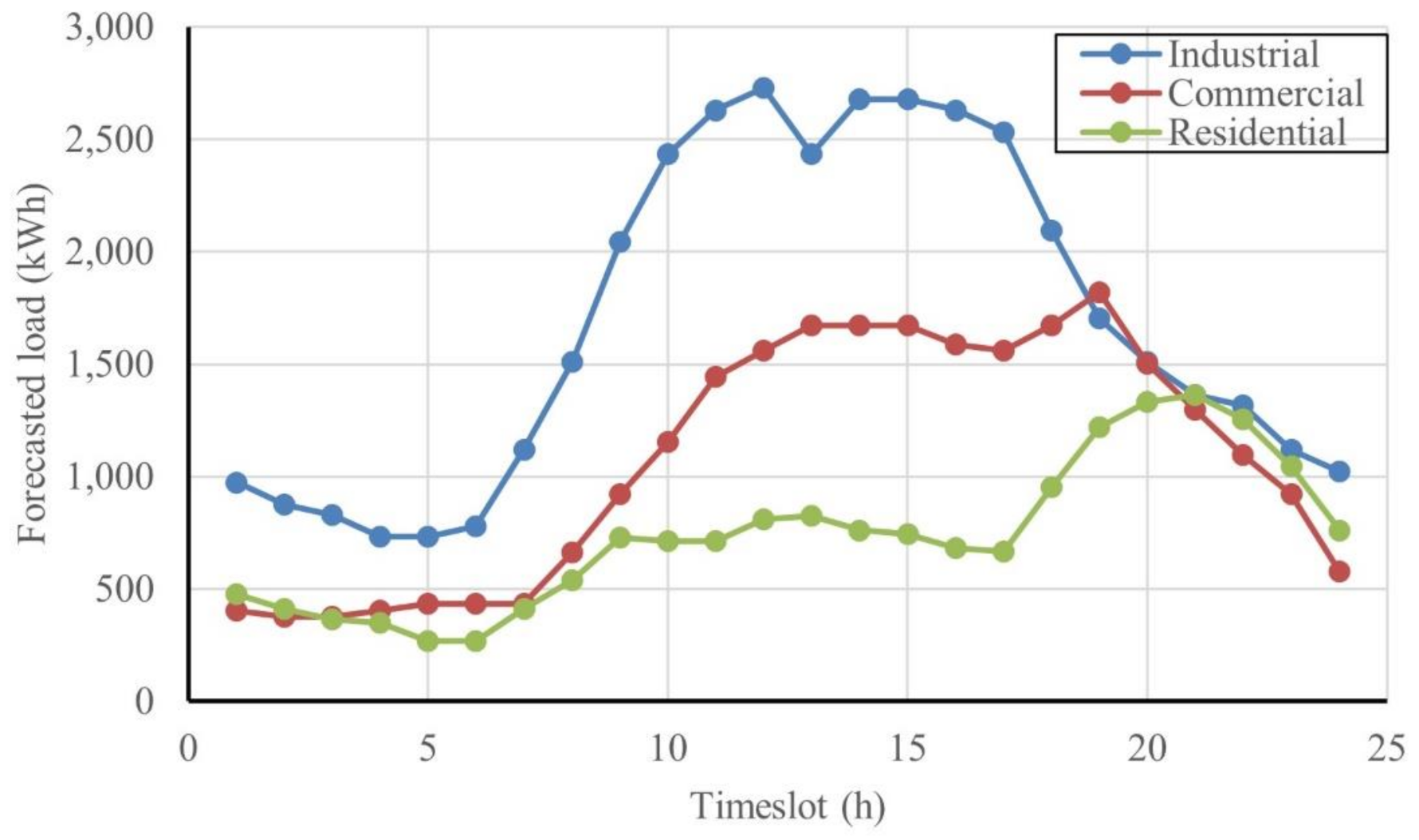
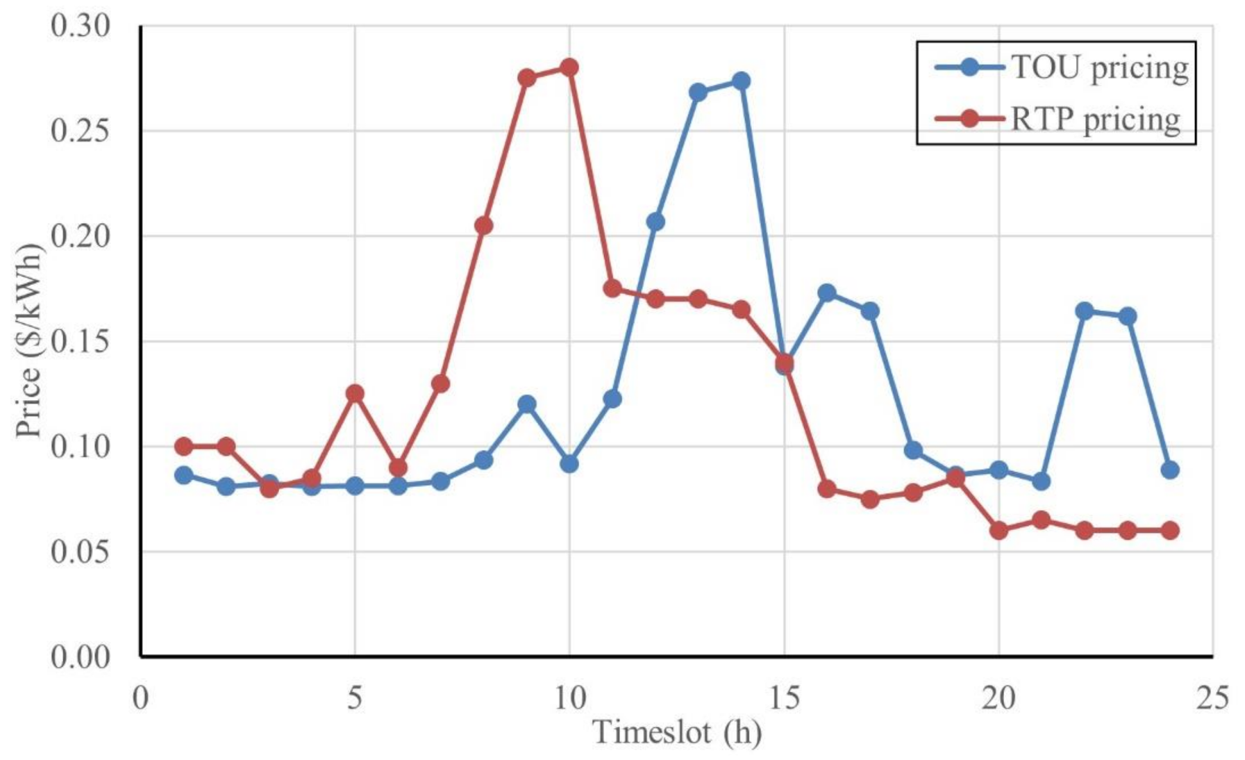
| Time (h) | TOU Pricing ($/kWh) | RTP Pricing ($/kWh) | Forecasted Load in the Residential Area (kWh) | Forecasted Load in the Industrial Area (kWh) |
|---|---|---|---|---|
| 24–1 | 0.0865 | 0.100 | 475.7 | 974.0 |
| 1–2 | 0.0811 | 0.100 | 412.3 | 876.6 |
| 2–3 | 0.0825 | 0.080 | 364.7 | 827.9 |
| 3–4 | 0.0810 | 0.085 | 348.8 | 730.5 |
| 4–5 | 0.0814 | 0.125 | 269.6 | 730.5 |
| 5–6 | 0.0813 | 0.090 | 269.6 | 779.2 |
| 6–7 | 0.0834 | 0.130 | 412.3 | 1120.1 |
| 7–8 | 0.0935 | 0.205 | 539.1 | 1509.7 |
| 8–9 | 0.1200 | 0.275 | 729.4 | 2045.5 |
| 9–10 | 0.0919 | 0.280 | 713.5 | 2435.1 |
| 10–11 | 0.1227 | 0.175 | 713.5 | 2629.9 |
| 11–12 | 0.2069 | 0.170 | 808.7 | 2727.3 |
| 12–13 | 0.2682 | 0.170 | 824.5 | 2435.1 |
| 13–14 | 0.2735 | 0.165 | 761.1 | 2678.6 |
| 14–15 | 0.1381 | 0.140 | 745.2 | 2678.6 |
| 15–16 | 0.1731 | 0.080 | 681.8 | 2629.9 |
| 16–17 | 0.1642 | 0.075 | 666.0 | 2532.5 |
| 17–18 | 0.0983 | 0.078 | 951.4 | 2094.2 |
| 18–19 | 0.0863 | 0.085 | 1220.9 | 1704.5 |
| 19–20 | 0.0887 | 0.060 | 1331.9 | 1509.7 |
| 20–21 | 0.0835 | 0.065 | 1363.6 | 1363.6 |
| 21–22 | 0.1644 | 0.060 | 1252.6 | 1314.9 |
| 22–23 | 0.1619 | 0.060 | 1046.5 | 1120.1 |
| 23–24 | 0.0887 | 0.060 | 761.1 | 1022.7 |
| Type of Devices | First-Hour Load (kWh) | Second-Hour Load (kWh) | Third-Hour Load (kWh) | Number of Devices |
|---|---|---|---|---|
| Water dispenser | 2.50 | - | - | 349 |
| Dryer | 3.50 | - | - | 168 |
| Electric kettle | 3.0 | 2.50 | - | 192 |
| Microwave oven | 5.0 | - | - | 255 |
| Coffee maker | 2.0 | 2.0 | - | 343 |
| Fan | 3.50 | 3.0 | - | 284 |
| AC | 4.0 | 3.5 | 3.0 | 245 |
| Lights | 2.0 | 1.75 | 1.50 | 156 |
| Total | 1992 | |||
| Type of Devices | Hourly Consumption of a Device | Number of Devices | ||
|---|---|---|---|---|
| First-Hour Demand (kWh) | Second-Hour Demand (kWh) | Third-Hour Demand (kWh) | ||
| Dryer | 1.20 | - | - | 308 |
| Dishwasher | 0.70 | - | - | 430 |
| Washing machine | 0.50 | 0.5 | - | 967 |
| Microwave oven | 1.30 | - | - | 375 |
| Iron box | 1.00 | - | - | 830 |
| Vacuum cleaner | 0.40 | - | - | 970 |
| Fan | 0.20 | 0.2 | 0.2 | 734 |
| Electric kettle | 2.00 | - | - | 752 |
| Toaster | 0.90 | - | - | 198 |
| Rice cooker | 0.850 | - | - | 277 |
| Hairdryer | 1.50 | - | - | 230 |
| Blender | 0.30 | - | - | 933 |
| Frying pan | 1.10 | - | - | 582 |
| Coffee maker | 0.80 | - | - | 221 |
| Total devices | 7807 | |||
| Pricing and Optimization | Cost before DSM ($) | Cost after DSM ($) | Cost Reduction (%) |
|---|---|---|---|
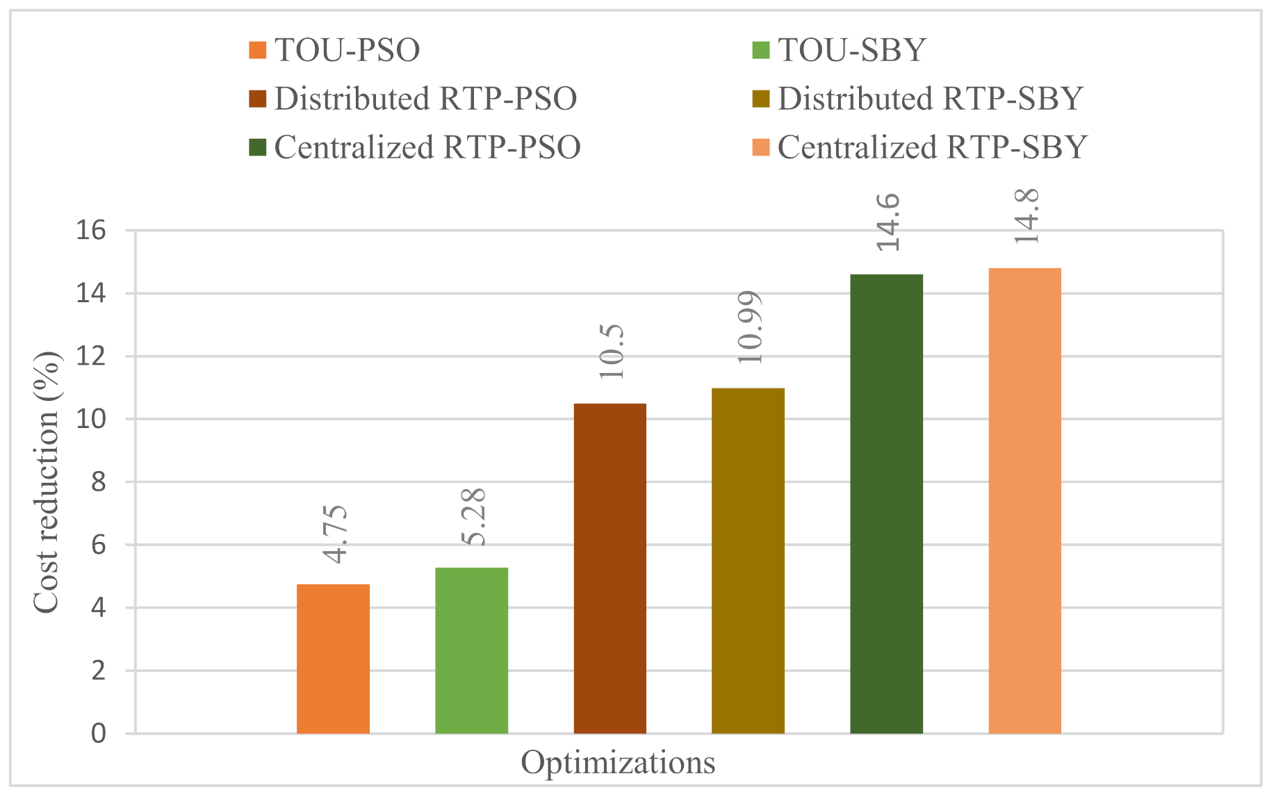
| TOU-PSO | 5423.271 | 5165.19 | 4.750 |
| TOU-SBY | 5137.09 | 5.280 | |
| Distributed RTP-PSO | 4855.70 | 10.50 | |
| Distributed RTP-SBY | 4827.20 | 10.99 | |
| Centralized RTP-PSO | 4632.36 | 14.60 | |
| Centralized RTP-SBY | 4621.00 | 14.80 |
| Pricing and Optimization | Cost before DSM ($) | Cost after DSM ($) | Cost Reduction (%) |
|---|---|---|---|
| TOU-PSO | 3636.60 | 3443.88 | 5.30 |
| TOU-SBY | 3437.90 | 5.46 | |
| Distributed RTP-PSO | 2994.00 | 17.70 | |
| Distributed RTP-SBY | 2973.00 | 18.20 | |
| Centralized RTP-PSO | 2885.26 | 20.70 | |
| Centralized RTP-SBY | 2847.70 | 21.70 |
| Pricing and Optimization | Cost before DSM ($) | Cost after DSM ($) | Cost Reduction (%) |
|---|---|---|---|
| TOU-PSO | 2302.879 | 2168.06 | 5.85 |
| TOU-SBY | 2128.71 | 7.56 | |
| Distributed RTP-PSO | 1871.30 | 18.74 | |
| Distributed RTP-SBY | 1842.50 | 19.99 | |
| Centralized RTP-PSO | 1814.80 | 21.19 | |
| Centralized RTP-SBY | 1799.90 | 21.84 |
| Pricing and Optimization | PAR |
|---|---|
| TOU-PSO | 1.852 |
| TOU-SBY | 1.825 |
| Distributed RTP-PSO | 1.770 |
| Distributed RTP-SBY | 1.729 |
| Centralized RTP-PSO | 1.760 |
| Centralized RTP-SBY | 1.712 |
| Pricing and Optimization | PAR |
|---|---|
| TOU-PSO | 1.684 |
| TOU-SBY | 1.646 |
| Distributed RTP-PSO | 1.543 |
| Distributed RTP-SBY | 1.525 |
| Centralized RTP-PSO | 1.477 |
| Centralized RTP-SBY | 1.422 |
| Pricing and Optimization | PAR |
|---|---|
| TOU-PSO | 1.607 |
| TOU-SBY | 1.589 |
| Distributed RTP-PSO | 1.421 |
| Distributed RTP-SBY | 1.415 |
| Centralized RTP-PSO | 1.426 |
| Centralized RTP-SBY | 1.409 |
Publisher’s Note: MDPI stays neutral with regard to jurisdictional claims in published maps and institutional affiliations. |
© 2021 by the authors. Licensee MDPI, Basel, Switzerland. This article is an open access article distributed under the terms and conditions of the Creative Commons Attribution (CC BY) license (https://creativecommons.org/licenses/by/4.0/).
Share and Cite
Ahmed, E.M.; Rathinam, R.; Dayalan, S.; Fernandez, G.S.; Ali, Z.M.; Abdel Aleem, S.H.E.; Omar, A.I. A Comprehensive Analysis of Demand Response Pricing Strategies in a Smart Grid Environment Using Particle Swarm Optimization and the Strawberry Optimization Algorithm. Mathematics 2021, 9, 2338. https://doi.org/10.3390/math9182338
Ahmed EM, Rathinam R, Dayalan S, Fernandez GS, Ali ZM, Abdel Aleem SHE, Omar AI. A Comprehensive Analysis of Demand Response Pricing Strategies in a Smart Grid Environment Using Particle Swarm Optimization and the Strawberry Optimization Algorithm. Mathematics. 2021; 9(18):2338. https://doi.org/10.3390/math9182338
Chicago/Turabian StyleAhmed, Emad M., Rajarajeswari Rathinam, Suchitra Dayalan, George S. Fernandez, Ziad M. Ali, Shady H. E. Abdel Aleem, and Ahmed I. Omar. 2021. "A Comprehensive Analysis of Demand Response Pricing Strategies in a Smart Grid Environment Using Particle Swarm Optimization and the Strawberry Optimization Algorithm" Mathematics 9, no. 18: 2338. https://doi.org/10.3390/math9182338